Robust in Practice: Adversarial Attacks on Quantum Machine Learning
Abstract
State-of-the-art classical neural networks are observed to be vulnerable to small crafted adversarial perturbations. A more severe vulnerability has been noted for quantum machine learning (QML) models classifying Haar-random pure states. This stems from the concentration of measure phenomenon, a property of the metric space when sampled probabilistically, and is independent of the classification protocol. In order to provide insights into the adversarial robustness of a quantum classifier on real-world classification tasks, we focus on the adversarial robustness in classifying a subset of encoded states that are smoothly generated from a Gaussian latent space. We show that the vulnerability of this task is considerably weaker than that of classifying Haar-random pure states. In particular, we find only mildly polynomially decreasing robustness in the number of qubits, in contrast to the exponentially decreasing robustness when classifying Haar-random pure states and suggesting that QML models can be useful for real-world classification tasks.
I Introduction
Quantum machine learning (QML) protocols, by exploiting quantum mechanics principles, such as superposition, tunneling, and entanglement Biamonte et al. 2017, have given hope of outperforming their classical counterparts, even with noisy intermediate-scale quantum (NISQ) Preskill 2018 hardware in the near-term Xia et al. 2020. For classification tasks where statistical patterns can be revealed in complex feature spaces, the high-dimensional Hilbert space of sizable quantum systems offers a naturally advantageous starting ground for QML models. However, many state-of-the-art classical machine learning models, such as deep neural networks with complicated internal feature mappings, have been shown vulnerable to small crafted perturbations to the input, namely adversarial examples Szegedy et al. 2014; Goodfellow et al. 2015. These are intentional worst-case perturbations to the original samples with an imperceptible difference that are nevertheless misclassified by the classifier. This not only raises questions as to why well-performing classifiers suffer from such instabilities but also poses security threats to machine learning applications that emphasize reliability, such as in spam filtering Dalvi et al. 2004. To understand this unreliable behavior, the transferability of these attacks across different architecture and the robustness against perturbations has led to extensive investigations in the classical machine learning community in recent years Chakraborty et al. 2018; Biggio and Roli 2018; Huang et al. 2011. Notably, some geometric and probabilistic arguments, based on curvatures of decision boundaries Fawzi et al. 2016 and the concentration of measure Mahloujifar et al. 2019; Gilmer et al. 2018; Diochnos et al. 2018; Fawzi et al. 2018a; Fawzi et al. 2018b, have been employed to quantify the risk of adversarial attacks in various settings. It has been shown that any classifier will have an adversarial robustness that is increasingly reduced by the dimension of the space on which it classifies, given the concentration of measure phenomenon in certain metric probability spaces Mahloujifar et al. 2019. This has raised attention in the QML community where the models take advantage of the high dimensionality of quantum systems Liu and Wittek 2020; Lu et al. 2020; Du et al. 2020; Guan et al. 2020
The concentration of measure is a phenomenon that describes the fact that, in certain metric probability spaces, points tend to gather around the boundaries of subsets having at least one half of the probability measure. As a result, there is generically a high probability of obtaining values close to the average for any reasonably smooth function that is evaluated on the distribution Ledoux 2001; Vitali D. Milman, Gideon Schechtman 2002; McClean et al. 2018; Popescu et al. 2006; Müller et al. 2011. This means that when samples are selected from such a concentrated space, the confidences predicted by the classifier tends to accumulate around the critical value separating the correct and incorrect classes. As such, small targeted perturbations can then easily move the samples across the decision boundary. In particular, it has been recognized that this phenomenon can lead to extreme vulnerabilities of any quantum classifier on high-dimensional Haar-random pure states Liu and Wittek 2020. Nevertheless, there is no indication of whether such vulnerability exists when classifying on a subset of encoded pure states in a realistic task, such as using a quantum classifier on classical images encoded in pure states.
In this paper, we approach the task of classifying quantum states from a geometric perspective. The quantum classifier divides the Hilbert space into subsets, each of which belongs to a certain class. We use this perspective here to study aspects of the problem that are relevant to practical applications of QML. In a practical classification task, such as in recognizing natural images, the samples to be classified can be generated from a Gaussian latent space by one of a number of commonly-used generative models Rezende and Mohamed 2015; Kingma and Welling 2014; Dinh et al. 2017; Goodfellow et al. 2014; Bojanowski et al. 2018; Arjovsky et al. 2017. The success of these models for real-world data generation ensures that the focus on QML models classifying a subset of encoded pure states, where these states are sampled from a distribution that is smoothly mapped from a Gaussian latent space Fawzi et al. 2018b, will yield insight into the vulnerability of QML models in a real-world classification task. This contrasts with the previous analysis of the vulnerabilities when classifying Haar-random pure states Liu and Wittek 2020.
We demonstrate that the adversarial robustness over this generated distribution decreases as in the number of qubits , with the scaling measured in the trace norm. This decline in the robustness is mild, indicating a quantum classifier can be robust to attacks on high dimensional quantum states. In contrast, when considering prediction-change adversarial settings where the inputs are pure states drawn Haar-randomly, we show that the robustness decreases as in the number of qubits , implying extreme vulnerabilities to attacks in high-dimensional quantum systems. This second case parallels the result of reference Liu and Wittek 2020, which considered error-region adversarial settings and found the robustness also decreases as here. However, we argue that the extreme vulnerability in this setting is not of concern in practice, since the states to be classified are always sampled from a distribution over some subsets of states, rather than from the Haar-random distribution over the entire set of pure states.
The rest of the paper is structured as follows. In Section II, we introduce the set-ups and preliminaries in both classical and quantum adversarial attacks. In Section III, we describe the prediction-change adversarial setting, which is often more relevant to real-world classification tasks than the previously employed error-region adversarial setting. We then derive the prediction-change adversarial robustness of any quantum classifier on Haar-randomly distributed pure states and explain its practical limitations. In Section IV, we derive the main results on the adversarial robustness of any quantum classifier classifying a smoothly generated distribution over a subset of encoded pure states of interest, and propose a feasible modification to any quantum classifier to lower bound unconstrained adversarial robustness. In Section V, a summary and discussion of the derived robustness over the two types of distribution are presented.
II Background
II.1 Classical Adversarial Attacks
Classical adversarial attacks were introduced to analyze the instability of deep neural networks caused by a small change to the input sample. Classically, the confidence is often quantified as the probability corresponding to the label class in the output normalized discrete distribution, e.g., the largest softmax value in the output vector in a multi-class logistic-regression convolutional neural network. As numerically shown in various works, such an attack results in a significant drop in the confidence in the correct class Szegedy et al. 2014; Kurakin et al. 2017; Kurakin et al. 2019; Biggio and Roli 2018, and may also bring a significant increase in the confidence in the incorrect class Goodfellow et al. 2015. So far, some arguments have been proposed to explain the vulnerabilities of various classifiers to adversarial attacks and their transferability Goodfellow et al. 2015; Bubeck et al. 2019; Charles et al. 2018; Engstrom et al. 2019; Fawzi et al. 2018a, yet no conclusive consensus has been established Göpfert et al. 2020.
The most common type of adversarial attack is the evasion attack where the adversary does not interfere with the training phase of a classifier and perturbs only the testing samples Chakraborty et al. 2018. The adversary can devise white-box attacks if it possesses total knowledge about the classifier architecture, or otherwise, it can devise black-box attacks relying on the transferability Chakraborty et al. 2018; Biggio and Roli 2018. We shall focus on white-box evasion attacks.
We introduce some notations and definitions used in this paper. Let denote the sample set with a metric and a probability measure . The notation denotes that a sample is drawn with a probability measure . denotes the countable label set. For a subset , we let and let be the -neighborhood of , where is the metric on . We also let be the -expansion of . is a hypothesis or a trained classifier that maps each to a predicted label . is the ground-truth function that maps each to a correct label . denotes the set of samples classified as label , namely . The error region is the set of samples on which the hypothesis disagrees with the ground-truth, namely . We define the risk as .
The two relevant types of evasion attacks studied here are based on the error region and the prediction change. In an error-region attack, the ground-truth function is accessible and an attack occurs when a perturbation in the sample causes to disagree with . In contrast, a prediction-change attack emphasizes the instability of : an attack occurs when a perturbation results in a different prediction by , and is irrelevant. The precise definitions of these two types of attacks are as follows.
Definition 1 .
The error-region adversarial risk under -perturbation is the probability of drawing a sample such that its -neighborhood intersects with the error region,
Definition 2 .
The prediction-change adversarial risk under -perturbation is the probability of drawing a sample such that its -neighborhood contains a sample with a different label,
equivalently,
In either type of attack, we call the nearest misclassified examples as the adversarial examples. We say that is more robust if the induced risk of either type is lower for a certain -perturbation. We shall refer to the minimal -perturbation to resulting in an adversarial example as the adversarial perturbation or the robustness of with . In contrast, we shall quantify the adversarial robustness of as the size of necessary for the adversarial risk of to be upper bounded by some constant. The main result of this paper is an upper bound on the adversarial robustness of any quantum classifier when the input states are smoothly generated from a Gaussian latent space.
II.2 Quantum Adversarial Attacks
For our work, a quantum classifier is a quantum channel that assigns labels with some set of positive-operator-valued measures (POVMs) . The quantum classifier takes in an ensemble of identically prepared copies of a state and assigns the state a label . The confidence of a prediction is quantified as the expectation value of the POVM for the prediction , namely for an input density matrix . We do not consider the number of copies of a state that is required to implement any specific quantum classification protocol. To measure the perturbation size, the natural choice of metric on quantum states – the trace distance – can be shown to generate an upper bound on the difference between their quantum classification confidence (see Appendix A), which implies that no small variation can induce a large swing in the predictive confidence. This property of the trace distance is a consequence of its interpretation as the achievable upper bound on the total variation distance 11 1 Informally, total variation distance is the largest possible difference between the probabilities that the two distributions can assign to the same event. between probability distributions arising from measurements performed on those quantum states Nielsen and Chuang 2010. Furthermore, we show in Appendix A that the Hilbert-Schmidt norm, the Bures distance, and the Hellinger distance between two quantum states all generate a similar upper bound. As a result, in quantum adversarial attacks, the adversary either perturbs the states near the decision boundary minimally to seek misclassification, or aims to maximize confidence change to any state with associated perturbations that are upper bounded by some considerable size in these norms, as illustrated in Figure 1. Our work analyzes primarily the risks due to the former objective. In Appendix B, we also propose a method for the latter objective exploiting the reversibility of parametrized quantum circuits (see e.g. Huggins et al. 2019; Benedetti et al. 2019). We note that the latter adversarial setting is justified, since in order to assess the security of a classifier under attack, it is reasonable – given a feasible space of modifications to the input data – to assume that the adversary aims to maximize the classifier’s confidence in wrong predictions, rather than merely perturbing minimally in size Biggio and Roli 2018.
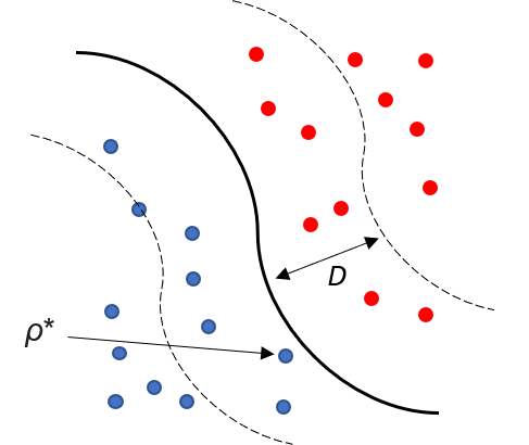
There are two natural set-ups of adversarial attacks in QML that can be specified. The first is when the input data to the classifier is already quantized and any data transmitted through the quantum communication network comes from an untrusted party. In this case, the adversary, who may be the sender or an interceptor, can perform an attack either by perturbing each of the transmitted density matrices, or by intercepting a fraction of the copies of the state and substituting them entirely (see Appendix A). In a broader context, our analysis can be extended to include the instability of classifying quantum states subject to decoherence. We focus on this first set-up in the current paper. The second set-up is when the input to the quantum classifier is classical. The quantum classifier encodes the classical data before classifying. Since the adversary is perturbing the classical input data, it is effectively attacking classically. If one views such a quantum classifier as a black-boxed hypothesis function that maps each input to a class, any classifier-agnostic classical analysis of adversarial robustness can then be directly applied. For example, reference Fawzi et al. 2016 analyzes the robustness of any classifier against random or semi-random perturbations, provided the curvature of the decision boundary is sufficiently small, while reference Fawzi et al. 2018b analyzes the adversarial robustness of any classifier when classical input vectors are smoothly mapped from a Gaussian latent representation.
II.3 Quantum Data Encoding
We now explain the feature maps used throughout the paper. Considering a normalized positive vector of length , without loss of generality, we intuitively refer to it as a gray-scale image with pixels in this paper. We focus on a particular set of encoding schemes where the normalized gray-scale value of each pixel, i.e., , is featurized into a qubit-encoding state . The product state to be classified is a tensor product state of these qubit-encoded pixels in the -dimensional Hilbert space Stoudenmire and Schwab 2016; Grant et al. 2018; Cao et al. 2020; Martyn et al. 2020, namely
| (1) |
The qubit-encoding states, Eq. (1), do not require a quantum random access memory (QRAM) Giovannetti et al. 2008 and are efficient in time to prepare. Other schemes including amplitude encoding (see e.g., Larose and Coyle 2020) are not considered here. We note that some of our results are general and independent of the encoding scheme. We further generalize Eq. (1) to qudits. In this case each pixel is mapped to a Hilbert space of higher dimension , with the coefficient of the -th component of the -th qudit state given by
| (2) |
These qudit states are special cases of what are known as spin-coherent states Stoudenmire and Schwab 2016, and the qubit states in Eq. (1) correspond to .
II.4 Concentration of Measure Phenomenon
To describe this phenomenon, let be a Borel set 22 2 Borel sets are sets that can be constructed from open or closed sets through countable union, countable intersection, and relative complement. The concentration function, defined as
| (3) |
has a smaller value when more points are aggregated in the -expansion of a sufficiently large set , for a fixed . Informally, a space exhibits a concentration of measure if decays very fast as grows, and we shall refer to it as a concentrated space. This is true for a simple example – the standard Gaussian distribution . Looking at the Borel set whose probability measure is , the cumulative density outside its -expansion, namely , decreases at least as fast as by the tail bound Vershynin 2017. One can invoke isoperimetric inequality Borell 1975 to show that this clustering occurs around any Borel set with measure at least and applies to any canonical -dimensional Gaussian measure in the Euclidean space (see Appendix G). More formally, a family of -dimensional spaces with corresponding concentration functions is called a (, )-normal Lévy family if , where and are particular constants. Consequently, the measure is more concentrated for a higher dimension. Two notable normal Lévy families are and , both of which are equipped with the Hilbert-Schmidt norm and the Haar probability measure Gromov and Milman 1983; Giordano and Pestov 2007. An implication of this phenomenon is that when points are drawn from a highly concentrated space, for any function varying not rapidly, we have with high probability. Lévy’s Lemma Ledoux 2001; Vitali D. Milman, Gideon Schechtman 2002 constitutes a specific example of this.
II.5 Related Work
The work in Mahloujifar et al. 2019 considered any normal Lévy family and derived the robustness for error-region adversarial attacks. The results show that for a nice classification problem 33 3 The precise definition of a nice classification problem can be found in Definition 2.3 in Mahloujifar et al. 2019., if , the size of perturbations must be in order to have the error-region adversarial risk upper bounded by some constant, where is the dimension of the concentrated space. References Diochnos et al. 2018; Gilmer et al. 2018 studied some specific concentrated spaces and revealed the same scaling.
Reference Liu and Wittek 2020 transforms the classification of pure states into that of unitaries in for some fixed initial state . These quantum classifiers then classify samples drawn from equipped with the Haar probability measure and the Hilbert-Schmidt norm, which is a -normal Lévy family. Therefore, if , the necessary condition on the perturbation size for the error-region adversarial risk to be bounded above by for some is . Precisely, to have , the -perturbation to any unitary must be upper bounded as 44 4 A concise proof of Eq. (4) can be found in Appendix C.
| (4) |
III Problems with Practical Classifications
The result in Eq. (4) claims that when classifying unitaries in with the Haar measure, given that an adversary can devise white-box attacks and not exponentially suppressed by , the robustness of any quantum classifier decreases polynomially in the dimension of the input . This is daunting since the input has a dimension exponential in the number of qudits.
To apply any result related to Eq. (4), a ground-truth function on is needed to obtain the risk . However, may not be easily defined in a real-world machine learning task. For instance, it is challenging to define what constitutes a mistake for visual object recognition. After adding a perturbation to an image, it likely no longer corresponds to a photograph of a real physical scene Elsayed et al. 2018. Furthermore, it is difficult to define the labels for images undergoing gradual semantic change. All of these factors complicate the evaluation of . It thus motivates us to focus on prediction-change adversarial risks (see e.g., Diochnos et al. 2018; Elsayed et al. 2018; Fawzi et al. 2016) in order to avoid requiring access to the ground-truth. The following theorem and corollary then apply.
Theorem 1 .
Let be equipped with the Haar measure and the Hilbert-Schmidt norm . For any hypothesis that is not a constant function, let determine the measure of the dominated class such that . Suppose , and a perturbation occurs, where . If the prediction-change adversarial risk , then must satisfy
| (5) |
It is evident from Eq. (5) that the upper bound on the size of the perturbation is suppressed as the dimension of the space increases. It is also suppressed when the measure of the dominated class () decreases and when the tolerance on the adversarial risk () decreases.
Corollary 1 .
The proofs can be found in Appendix D and E. The interpretation of Theorem 1 and Corollary 1 is clear: given that no class occupies Haar-measure , any quantum classifier on quantum states is more vulnerable to prediction-change adversarial attacks on higher-dimensional pure states drawn Haar-randomly, with the robustness decaying exponentially in the number of qudits.
In what follows, we apply this theorem to a practical task by presenting two perspectives on the application, in order to illustrate the limitations of the theorem. Suppose that the objective of the practical task is to classify a subset of quantum states, for example, the pure product states in Section II.3 that encode images displaying a digit or . On one hand, if we label unitaries not related to an actual image, together with unitaries associated with noisy images not displaying a digit 0 or 1, in a third-class, this class will have measure 1, since the set of all unitaries that evolve the initial to some final pure product state has Haar measure 0 in Lockhart 2002. For example when , this can be seen by recognizing that the encoded states correspond to only a fraction of the circle going through and on the Bloch Sphere. This labeling renders Theorem 1 useless for any trained in this way because . On the other hand, if we train a binary to classify half of , including unitaries corresponding to 0-digit images, to , and the other half, including unitaries corresponding to 1-digit images, to , then . Using Eq. (5) then gives robustness against prediction-change adversarial attacks, again suggesting extreme vulnerabilities in high dimensions.
However, the interpretation of this result is not of practical interest, for the following reasons. We emphasize that in applying Theorem 1 or Eq. (4), the notion of adversarial risks by Definition 2 represents the probability of perturbing a Haar-randomly selected unitary by some to its adversarial example. It does not represent, for instance, the probability of perturbing a particular unitary associated with a real image to its adversarial example, nor does it represent the risk of attacking a unitary drawn from any other distribution over some subset. Therefore, if the task is to train and generalize a quantum classifier on a subset of quantum states with some distribution, this theorem cannot claim vulnerabilities that are exponential in the number of qudits. It is also noted that, as far as how Eq. (4) and Theorem 1 are formulated, the perturbed states cannot be mixed states since these are mapped from by a completely positive and tracing preserving (CPTP) maps rather than by unitaries. In Section IV, we shall see that this is an example of an in-distribution attack, which applies to scenarios where both the original and perturbed states are pure.
IV Classifications on Generator Output Distributions
IV.1 Concentration in Generated Distributions
In practice, one is interested in the performance of a classifier on a distribution over some subset of meaningful samples, such as the subset of images displaying digits including the MNIST data set. It is this distribution on which the adversarial risk should be computed in order to infer the extent of the vulnerability. To ensure that the probability measure on the classifier-input space covers meaningful samples, we resort to approximating the distribution over meaningful samples using the image of a smooth generator function on a concentrated latent space, trained on samples of interest Fawzi et al. 2018b. Following convention, we refer to the latter as a real-data manifold. Such a generator can be a Normalizing Flow model Rezende and Mohamed 2015; Kingma and Welling 2014; Dinh et al. 2017 or the generator of a Generative Adversarial Network (GAN) Goodfellow et al. 2014; Bojanowski et al. 2018; Arjovsky et al. 2017, both with a Gaussian latent space, trained on the same data set that the classifier will be trained on. A generative model serving this purpose is also referred to as a spanner Jalal et al. 2019. In this way, a major fraction of the samples in the generator output can be related to samples of interest, despite the fact that, the smoothness of the generator may introduce some samples off the real-data manifold, such as those undergoing gradual semantic change during interpolations. This generative set-up can be generalized to multiple generators on the same latent space. However, each generator maps to a disjoint part of the real-data manifold, overcoming the problem of covering the off real-data manifold when the latent space is globally connected Khayatkhoei et al. 2018. This generalization requires relaxing the demand that in the Eq. (6) below. As a result, no data off the real-data manifold is generated in .
The reason that we require the latent space to be concentrated is so that we can study the concentration of samples in the generator-output space resulted from the concentration of the latent space. This connection is made by the assumption that the generator is smooth, in the sense that it admits a modulus of continuity (i.e., it is uniformly continuous), namely if there exists a monotone invertible function such that
| (6) |
where is the metric equipped by the image of . This is a weaker condition than the Lipschitz continuity which results when is a linear function. In this paper, we assume to yield a tight upper bound in Eq. (6), and we demand to be small for small for a smooth generator. The idea is that any tendency to concentration of measure in the latent space is preserved by such a smooth mapping to its image, and the generated samples then follow a modified concentrated distribution. We can imagine that if some pairs of latent variables from different classes are within distance across the class boundary in the generator domain, their generator images must be accordingly within distance at most across the boundary. This can also display a clustering. Although the tendency to cluster is preserved, the extent to which the points in the generator image gather is mediated by the modulus of continuity. A tight upper bound with that yields distances larger than the typical distances in the output space means that generated samples can be further apart, and vice versa. As far as adversarial robustness is concerned, a larger is then favorable since it implies that larger perturbations are needed to definitively perturb a larger number of generated samples across decision boundaries.
In generating these to-be-classified samples, the fact that a large probability density resides near the decision boundary is not at odds with a trained classifier that predicts training samples with high confidence. The training samples comprise only a subset of the support of the generator-output distribution. High confidence training samples result from the classifier drawing the decision boundaries away from them. When such a decision boundary encloses a sufficiently large measure, it then inevitably encounters large probability densities – as dictated by the concentration of measure phenomenon on these distributions – that do not contribute to training. As a result, when generalizing to test samples that are similar to the training samples, some test samples may locate near the boundary and be the vulnerable targets to adversarial attacks.
IV.2 Robustness of QML Models
We consider the quantum adversarial attack set-up where the input to the classifier is already quantized and transmitted through a quantum communication network.
Let our latent space be, for example in this paper, the with the Euclidean metric and the canonical -dimensional Gaussian measure so it is a concentrated space. Let in . Suppose that a smooth generator is trained to generate a distribution of concern, such as some distribution of natural images, on a subset of . For a sample , we then have .
Incorporated in the generator , maps the latent space to a subset of -pixel natural images, then encodes the natural image into a density matrix defined in Eq. (2). That is, , where – the image of – is a subset of all density matrices . The metric on density matrices is the trace norm unless otherwise specified. The probability measure , which is a distribution mapped by from the -dimensional Gaussian measure on , is only supported on over density matrices capturing the natural image distribution. Any quantum classifier then classifies the density matrices in . Let us denote the intermediate stage – the set of images with pixels (normalized vectors with length n) – as , then the corresponding measure on can be denoted as . The metric on is, for instance, the norm. Diagrammatically, these mappings are
It is noted that smoothness is a desirable property of generative models. It is hinted at gradual transitions in the features in the generated samples, which imply that the generator has learned relevant factors of variation Radford et al. 2016. We are then justified in assuming that the real-data manifold on can be covered by a smooth generator (see e.g., Kingma and Welling 2014; Dinh et al. 2017; Goodfellow et al. 2014; Bojanowski et al. 2018; Arjovsky et al. 2017). In what follows, we show that the overall generator , mapping from to the real-data manifold in the set of density matrices , is also smooth.
Proposition 1 .
Assuming that is smooth with a modulus of continuity and the qudit encoding scheme, Eq. (2), is applied, then the generator is also smooth and admits a modulus of continuity that is lower bounded as
The proof can be found in Appendix F. In terms of the scaling with respect to and , when scales as , for instance, when is Lipschitz continuous (e.g., the generator in Behrmann et al. 2019; Zhang et al. 2019), Proposition 1 implies that the modulus of continuity of the overall generator , i.e., , scales as . It is desirable to enforce Lipschitz continuity on some generators, for example when imposing spectral normalization Miyato et al. 2018 on the generator of a GAN to improve training Zhang et al. 2019.
A distinction can be made concerning whether the adversarial example must be also in the subset . If so, the adversarial attack is called in-distribution, since the attacker only looks for an adversarial example within the data manifold . Otherwise, we call it an unconstrained adversarial attack since the perturbation is arbitrary in , i.e., it is not confined to the data manifold. We state the precise definitions, based on prediction-change adversarial risks in Definition 2, as follows.
Definition 3 .
An in-distribution adversarial attack, or a data-manifold attack, attempts to find the perturbation
which is within the data manifold . It induces an in-distribution adversarial risk,
Definition 4 .
An unconstrained adversarial attack attempts to find
which is in not restricted to the data manifold . It induces an unconstrained adversarial risk,
It is noted that when the generator is surjective on , i.e., , there is no distinction between the two types of attacks.The set-ups in Theorem 1 and Eq. (4) consider classifying on the subset of all pure-state density matrices in on which a Haar-random distribution is supported. Since this requires both the original and perturbed states be pure, the adversarial risks are considered in-distribution, although we shall see in Section IV.2 that the same upper bound applies to the unconstrained robustness for a general quantum classifier.
In-distribution Adversarial Robustness
The following theorem, depending on the distribution to be classified as well as the specific classical-data generator in terms of , then applies.
Theorem 2 .
Let be any quantum classifier on the set of density matrices. Considering in-distribution adversarial attacks on the image of , if , i.e., the classes are not too unbalanced, then for the prediction-change risk , the distance between two density matrices must satisfy
| (7) |
where is the modulus of continuity in Proposition 1.
The proof can be found in Appendix G. This result is independent of the quantum data encoding scheme. It can be generalized to quantum classifiers with arbitrary decision boundaries, but in this case, the necessary upper bound on the in-distribution robustness will not have a closed-form (see Appendix G). This upper bound is saturated when Eq. (6) is tight and the quantum classifier induces linearly separable regions in the latent space, namely when is a linear function on , giving rise to the maximally robust quantum classifier. The non-saturation of this upper bound when class regions are not linearly separable in can be seen in the example of the standard Gaussian in Section II.4 above. Suppose one looks at for some , which has the same probability measure as but is not linearly separable in . The measure outside the -expansion of , i.e., , is smaller than that outside of the -expansion of , namely , implying more concentration outside and near than .
The non-saturation of this upper bound for non-linearly separable classification regions in also implies that it is prone to misclassification with an increasing number of equiprobable classes. The proof for cases with at least 5 equiprobable classes can be found in Appendix G. Informally, more equiprobable classes lead to more boundaries, enclosing classes with sufficiently large total measure, that border distinct classes. Then within a fixed distance beyond more of those boundaries, there are more samples subject to some prediction change.
We note that this upper bound is usually not saturated in practice, since a quantum classifier is usually linear, such as a parametrized quantum circuit and a unitary tensor network, while the generator is usually non-linear, given that is usually non-linear and , the quantum feature map, is non-linear. Classically, some highly-nonlinear state-of-the-art neural networks have robustness one or two orders of magnitude smaller in the norm on some data sets than the corresponding upper bound derived with similar arguments Fawzi et al. 2018b. It would be interesting to examine the amount of deviation from the upper bound for QML models in future works.
Theorem 2 implies that when the quantum states to be classified encode classical data generated with a modulus of continuity scaling as , the in-distribution robustness of any quantum classifier decreases polynomially in the number of qudits and increases polynomially in the qudit dimension . To see this, we first note that according to Proposition 1, when , which applies to generators such as those enforcing Lipschitz continuity, is lower bounded by a function that scales as . This means that the upper bound on the perturbation size between any two in-distribution states, i.e., the right hand side of Eq. (7), is then asymptotically bounded from below by .
As such, the vulnerability increases slightly with a larger number of qudits and by contrast, decreases slightly with qudits of higher dimension . When the encoded classical data manifold comes from generators for which Lipschitz continuity is not enforced, it requires numerical approximations of the modulus of continuity to determine its scaling in the output space, before obtaining the robustness scaling. Compared to Theorem 1 where samples are Haar-random pure states, the states to be classified here, which characterise the adversarial risk, are similar to those considered in practical tasks. Specifically, they are a subset of encoded states with a distribution smoothly generated from a Gaussian latent space. Theorem 2 demonstrated that, contrary to previous claims Liu and Wittek 2020, there is no guarantee that quantum classifiers are exponentially more vulnerable to in-distribution attacks in higher-dimensional Hilbert space. We shall now show that the theorem applies to unconstrained attacks as well.
Unconstrained Adversarial Robustness
Unconstrained adversarial attacks are arbitrary perturbations in to a sample . In a broader context in which the instability of the quantum classifier is concerned, this may derive from density matrices subject to decoherence in a classification task. It is clear that and thus, it holds by changing the in-distribution perturbations in Theorem 2 to unconstrained ones, and the same bound in Eq. (7) applies.
We argue that there does not exist a tighter upper bound that holds for general quantum classifiers for unconstrained robustness. Consider a particular family of quantum classifiers that project any state onto the data manifold, namely to map any state to its closest in-distribution state, before classifying. These classifiers can be shown to satisfy 55 5 It is proven in Theorem 2 in Fawzi et al. 2018b.. Even in the worst case where , their unconstrained robustness is as large as half of the in-distribution one. We stress that, although robust, such a quantum classifier is inefficient in our setting since there is no apparent tractable way to obtain the closest pure product state to an arbitrary state.
Inspired by this strategy, we propose that one can construct a family of efficient quantum classifiers on -qubit density matrices with unconstrained robustness lower bounded for any . To be specific, we construct from any with the following procedure.
Let the original sample be a pure product-state density matrix with qudits as in Eq. (1). A perturbation leads to a sample . First, we perform single qubit tomography on every qubit of to reconstruct a product-state density matrix from these single qubits. We denote this mapping as . Subsequently, we numerically fit the pixel values to to find its closest density matrix within our data manifold . We use a symbol to represent the density matrix attained from this procedure. is then replacing when fed to the quantum classifier . We have the following theorem,
Theorem 3 .
For every -qubit , let be the density matrix within the data manifold attained from the above procedure. For any quantum classifier , let be such that , then
where for even and for odd .
The proof can be found in Appendix H. We note that the procedure can be applied to any product state encoding scheme. This procedure yields an explicit lower bound to the unconstrained adversarial perturbation when it is possible to estimate the in-distribution adversarial perturbation by, for example, sampling in the latent space Zhao et al. 2018 or gradient descent search in the latent space Jalal et al. 2019 before mapping to the density matrices. This constructed from amounts to a feasible tomographic preprocessing of input states. It guarantees that the unconstrained robustness of each sample is bounded from below and may be used as a defense strategy against unconstrained adversarial attacks in practice. However, we note that when is large, this lower bound can be several orders of magnitude smaller than the upper bound.
V Discussion
A summary of the upper bounds on the prediction-change adversarial robustness over pure states sampled from the Haar-random distribution and a smoothly generated distribution , is presented in Table 1.
In this work, we first showed the prediction-change adversarial robustness over Haar-randomly distributed pure states, and compared this with the previously demonstrated error-region robustness of Liu and Wittek 2020 over the same distribution. Both types of adversarial robustness show similar extreme vulnerabilities exponential in the number of qudits. However, in this work we have argued that these vulnerabilities for Haar-random pure states are not of practical interest. This is because, in practice, the adversarial risk of a quantum classifier should be computed on a distribution over some subset of meaningful states, such as a subset of qubit encoding states featurizing some images, in order to infer the extent of the vulnerability. In general, practical quantum classification tasks classify a subset of encoded states with some commonly used qubit encoding scheme. For such tasks, we have shown that we can use the concentration of measure phenomenon to derive the robustness of any quantum classifiers in situations where the distribution of states to be classified can be smoothly generated from a Gaussian latent space, as quantified in Eq. (6). In this situation, we have shown that one finds only a mildly polynomially decreasing robustness in the number of such encoded qubits, specifically with scaling as in the trace norm.
As noted for Theorem 2, it is the upper bound on the perturbation size necessary for the adversarial risk to be bounded from above that scales as . This upper bound is usually not tight and the actual adversarial robustness could therefore be smaller. We have also proposed a feasible modification of any quantum classifier with product-state inputs – namely, by performing single qubit tomography before numerically fitting the closest encoded qubit state – to obtain a lower bound on the unconstrained robustness and to defend against unconstrained adversarial attacks.
Most importantly, our analysis provides QML protocols some relief from adversarial attacks in real-world tasks. For example, when classifying on some qubit states encoding MNIST images, the robustness decreases only as , in contrast to the extreme vulnerability of quantum classifiers in classifying Haar-random pure states (Theorem 1 and Liu and Wittek 2020). In future, it will be interesting to experimentally compare the adversarial robustness of particular QML models for real-world data on a distribution of states smoothly mapped from a Gaussian latent space with the bounds that we have derived here.
We note that the polynomially decreasing robustness in is derived from the qudit encoding scheme. The concentration of measure due to the Gaussian isoperimetric inequality for the latent space only contributes to the argument of Eq. (7). It will be interesting to investigate whether a different encoding scheme can give better scaling in the robustness, and also to determine whether quantum data that derives naturally from a distribution other than the Haar-random distribution is robust to attacks. In Appendix B, we propose a method to perform white-box adversarial attacks on classically intractable input states with QML models. It will be interesting to further explore white-box attacks, assuming that the adversary is capable of devising these. In practice, with current NISQ-era hardware, it will also be useful to examine how robust QML models are against adversarial attacks under noise and decoherence.
Acknowledgement
H. L. was supported by the National Aeronautics and Space Administration under Grant/Contract/Agreement No.80NSSC19K1123 issued through the Aeronautics Research Mission Directorate. I.C. was supported by the US Department of Energy, Office of Science, Office of Advanced Scientific Computing Research, Quantum Algorithm Teams Program, under contract number DE-AC02-05CH11231. W. H. was supported by a grant from Siemens Corporation.
References
- Biamonte et al. (2017) Jacob Biamonte, Peter Wittek, Nicola Pancotti, Patrick Rebentrost, Nathan Wiebe, and Seth Lloyd, “Quantum machine learning,” Nature 549, 195–202 (2017).
- Preskill (2018) John Preskill, “Quantum Computing in the NISQ Era and Beyond,” Quantum 2, 79 (2018).
- Xia et al. (2020) Yi Xia, Wei Li, Quntao Zhuang, and Zheshen Zhang, “Quantum-enhanced Data Classification with a Variational Entangled Sensor Network,” arXiv: 2006.11962 (2020).
- Szegedy et al. (2014) Christian Szegedy, Wojciech Zaremba, Ilya Sutskever, Joan Bruna, Dumitru Erhan, Ian Goodfellow, and Rob Fergus, “Intriguing Properties of Neural Networks,” in ICLR (2014).
- Goodfellow et al. (2015) Ian J. Goodfellow, Jonathon Shlens, and Christian Szegedy, “Explaining and Harnessing Adversarial Examples,” in ICLR (2015).
- Dalvi et al. (2004) Nilesh Dalvi, Pedro Domingos, Mausam, Sumit Sanghai, and Deepak Verma, “Adversarial Classification,” in ACM (2004) p. 99.
- Chakraborty et al. (2018) Anirban Chakraborty, Manaar Alam, Vishal Dey, Anupam Chattopadhyay, and Debdeep Mukhopadhyay, “Adversarial Attacks and Defences: A Survey,” Procedia Computer Science 140 (2018).
- Biggio and Roli (2018) Battista Biggio and Fabio Roli, “Wild Patterns: Ten Years After the Rise of Adversarial Machine Learning,” Pattern Recognition 84, 317–331 (2018).
- Huang et al. (2011) Ling Huang, Anthony D. Joseph, Blaine Nelson, Benjamin I.P. Rubinstein, and J. D. Tygar, “Adversarial Machine Learning,” in ACM (2011) pp. 43–57.
- Fawzi et al. (2016) Alhussein Fawzi, Seyed-Mohsen Moosavi-Dezfooli, and Pascal Frossard, “Robustness of classifiers: from adversarial to random noise,” in NIPS (2016) pp. 1632–1640.
- Mahloujifar et al. (2019) Saeed Mahloujifar, Dimitrios I. Diochnos, and Mohammad Mahmoody, “The Curse of Concentration in Robust Learning: Evasion and Poisoning Attacks from Concentration of Measure,” in AAAI, Vol. 33 (2019) pp. 4536–4543.
- Gilmer et al. (2018) Justin Gilmer, Luke Metz, Fartash Faghri, Samuel S Schoenholz, Maithra Raghu, Martin Wattenberg, Ian Goodfellow, and Google Brain, “The Relationship Between High-Dimensional Geometry and Adversarial Examples,” arXiv:1801.02774v3 (2018).
- Diochnos et al. (2018) Dimitrios I. Diochnos, Saeed Mahloujifar, and Mohammad Mahmoody, “Adversarial Risk and Robustness: General Definitions and Implications for the Uniform Distribution,” in NIPS (2018) pp. 10380–10389.
- Fawzi et al. (2018a) Alhussein Fawzi, Omar Fawzi, and Pascal Frossard, “Analysis of Classifiers’ Robustness to Adversarial Perturbations,” Machine Learning 107, 481–508 (2018a).
- Fawzi et al. (2018b) Alhussein Fawzi, Hamza Fawzi, and Omar Fawzi, “Adversarial Vulnerability for Any Classifier,” in NIPS (2018) pp. 1186–1195.
- Liu and Wittek (2020) Nana Liu and Peter Wittek, “Vulnerability of Quantum Classification to Adversarial Perturbations,” Physical Review A 101 (2020).
- Lu et al. (2020) Sirui Lu, Lu-Ming Duan, and Dong-Ling Deng, “Quantum Adversarial Machine Learning,” Physical Review Research 2 (2020).
- Du et al. (2020) Yuxuan Du, Min-Hsiu Hsieh, Tongliang Liu, Dacheng Tao, and Nana Liu, “Quantum Noise Protects Quantum Classifiers Against Adversaries,” arXiv: 2003.09416 (2020).
- Guan et al. (2020) Ji Guan, Wang Fang, and Mingsheng Ying, “Robustness Verification of Quantum Machine Learning,” arXiv:2008.07230 (2020).
- Ledoux (2001) Michel Ledoux, The Concentration of Measure Phenomenon, Mathematical Surveys and Monographs, Vol. 89 (American Mathematical Society, 2001).
- Vitali D. Milman, Gideon Schechtman (2002) Vitali D. Milman, Gideon Schechtman, Asymptotic Theory of Finite Dimensional Normed Spaces: Isoperimetric Inequalities in Riemannian Manifolds, Lecture Notes in Mathematics (Springer, 2002).
- McClean et al. (2018) Jarrod R. McClean, Sergio Boixo, Vadim N. Smelyanskiy, Ryan Babbush, and Hartmut Neven, “Barren Plateaus in Quantum Neural Network Training Landscapes,” Nature Communications 9 (2018).
- Popescu et al. (2006) Sandu Popescu, Anthony J. Short, and Andreas Winter, “Entanglement and the Foundations of Statistical Mechanics,” Nature Physics 2, 754–758 (2006).
- Müller et al. (2011) Markus P. Müller, David Gross, and Jens Eisert, “Concentration of Measure for Quantum States with a Fixed Expectation Value,” Communications in Mathematical Physics 303, 785–824 (2011).
- Rezende and Mohamed (2015) Danilo Jimenez Rezende and Shakir Mohamed, “Variational Inference with Normalizing Flows,” in PMLR, Vol. 37 (2015) pp. 1530–1538.
- Kingma and Welling (2014) Diederik P. Kingma and Max Welling, “Auto-Encoding Variational Bayes,” in ICLR (2014).
- Dinh et al. (2017) Laurent Dinh, Jascha Sohl-Dickstein, and Samy Bengio, “Density Estimation Using Real NVP,” in ICLR (2017).
- Goodfellow et al. (2014) Ian J Goodfellow, Jean Pouget-Abadie, Mehdi Mirza, Bing Xu, David Warde-Farley, Sherjil Ozair, Aaron Courville, and Yoshua Bengio, “Generative Adversarial Nets,” in NIPS (2014) pp. 2672–2680.
- Bojanowski et al. (2018) Piotr Bojanowski, Armand Joulin, David Lopez-Paz, and Arthur Szlam, “Optimizing the Latent Space of Generative Networks,” in PMLR, Vol. 80 (2018) pp. 600–609.
- Arjovsky et al. (2017) Martin Arjovsky, Soumith Chintala, and Leon Bottou, “Wasserstein Generative Adversarial Networks,” in PMLR, Vol. 70 (2017) pp. 214–223.
- Kurakin et al. (2017) Alexey Kurakin, Ian J. Goodfellow, and Samy Bengio, “Adversarial Machine Learning at Scale,” in ICLR (2017).
- Kurakin et al. (2019) Alexey Kurakin, Ian J. Goodfellow, and Samy Bengio, “Adversarial Examples in the Physical World,” in ICLR (2019).
- Bubeck et al. (2019) Sébastien Bubeck, Eric Price, and Ilya Razenshteyn, “Adversarial Examples from Computational Constraints,” in PMLR, Vol. 97 (2019) pp. 831–840.
- Charles et al. (2018) Zachary Charles, Harrison Rosenberg, and Dimitris Papailiopoulos, “A Geometric Perspective on the Transferability of Adversarial Directions,” in PMLR, Vol. 89 (2018) pp. 1960–1968.
- Engstrom et al. (2019) Logan Engstrom, Justin Gilmer, Gabriel Goh, Dan Hendrycks, Andrew Ilyas, Aleksander Madry, Reiichiro Nakano, Preetum Nakkiran, Shibani Santurkar, Brandon Tran, Dimitris Tsipras, and Eric Wallace, “Adversarial Examples Are Not Bugs, They Are Features,” in NIPS (2019) pp. 125–136.
- Göpfert et al. (2020) Jan Philip Göpfert, André Artelt, Heiko Wersing, and Barbara Hammer, “Adversarial Attacks Hidden in Plain Sight,” Advances in Intelligent Data Analysis (2020).
- (37) Informally, total variation distance is the largest possible difference between the probabilities that the two distributions can assign to the same event.
- Nielsen and Chuang (2010) Michael A. Nielsen and Isaac L. Chuang, Quantum Computation and Quantum Information (Cambridge University Press, 2010).
- Huggins et al. (2019) William Huggins, Piyush Patil, Bradley Mitchell, K. Birgitta Whaley, and E. Miles Stoudenmire, “Towards Quantum Machine Learning with Tensor Networks,” Quantum Science and Technology 4, 24001 (2019).
- Benedetti et al. (2019) Marcello Benedetti, Erika Lloyd, Stefan Sack, and Mattia Fiorentini, “Parameterized Quantum Circuits as Machine Learning Models,” Quantum Science and Technology 4, 043001 (2019).
- Stoudenmire and Schwab (2016) E. Miles Stoudenmire and David J. Schwab, “Supervised Learning with Quantum-Inspired Tensor Networks,” in NIPS (2016) pp. 4799–4807.
- Grant et al. (2018) Edward Grant, Marcello Benedetti, Shuxiang Cao, Andrew Hallam, Joshua Lockhart, Vid Stojevic, Andrew G. Green, and Simone Severini, “Hierarchical Quantum Classifiers,” Quantum Information 4, 65 (2018).
- Cao et al. (2020) Shuxiang Cao, Leonard Wossnig, Brian Vlastakis, Peter Leek, and Edward Grant, “Cost-function Embedding and Dataset Encoding for Machine Learning with Parameterized Quantum Circuits,” Physical Review A 101, 052309 (2020).
- Martyn et al. (2020) John Martyn, Guifre Vidal, Chase Roberts, and Stefan Leichenauer, “Entanglement and Tensor Networks for Supervised Image Classification,” arXiv:2007.06082 (2020).
- Giovannetti et al. (2008) Vittorio Giovannetti, Seth Lloyd, and Lorenzo Maccone, “Quantum Random Access Memory,” Physical Review Letters 100, 160501 (2008).
- Larose and Coyle (2020) Ryan Larose and Brian Coyle, “Robust Data Encodings for Quantum Classifiers,” Physical Review A 102, 032420 (2020).
- (47) Borel sets are sets that can be constructed from open or closed sets through countable union, countable intersection, and relative complement.
- Vershynin (2017) Roman Vershynin, “Four lectures on probabilistic methods for data science,” arXiv:1612.06661 (2017).
- Borell (1975) Christer Borell, “The Brunn-Minkowski inequality in Gauss space,” Inventiones Mathematicae 30, 207–216 (1975).
- Gromov and Milman (1983) M. Gromov and V. D. Milman, “A Topological Application of the Isoperimetric Inequality,” American Journal of Mathematics 105, 843–854 (1983).
- Giordano and Pestov (2007) Thierry Giordano and Vladimir Pestov, “Some Extremely Amenable Groups Related to Operator Algebras and Ergodic Theory,” Journal of the Institute of Mathematics of Jussieu 6 (2007).
- (52) The precise definition of a nice classification problem can be found in Definition 2.3 in Mahloujifar et al. 2019.
- (53) A concise proof of Eq. (4) can be found in Appendix C.
- Elsayed et al. (2018) Gamaleldin F. Elsayed, Nicolas Papernot, Shreya Shankar, Alexey Kurakin, Brian Cheung, Ian Goodfellow, and Jascha Sohl-Dickstein, “Adversarial Examples That Fool Both Computer Vision and Time-limited Humans,” in NIPS (2018) pp. 3910–3920.
- Lockhart (2002) Robert Lockhart, “Low-rank Separable States Are A Set of Measure Zero Within the Set of Low-rank States,” Physical Review A 65, 064304 (2002).
- Jalal et al. (2019) Ajil Jalal, Andrew Ilyas, and Constantinos Daskalakis, “The Robust Manifold Defense: Adversarial Training using Generative Models,” arXiv: 1712.09196v5 (2019).
- Khayatkhoei et al. (2018) Mahyar Khayatkhoei, Maneesh K. Singh, and Ahmed Elgammal, “Disconnected Manifold Learning for Generative Adversarial Networks,” in NIPS (2018) pp. 7343–7353.
- Radford et al. (2016) Alec Radford, Luke Metz, and Soumith Chintala, “Unsupervised Representation Learning with Deep Convolutional Generative Adversarial Networks,” in ICLR (2016).
- Behrmann et al. (2019) Jens Behrmann, Will Grathwohl, Ricky T. Q. Chen, David Duvenaud, and Jörn-Henrik Jacobsen, “Invertible Residual Networks,” in PMLR, Vol. 97 (2019) pp. 573–582.
- Zhang et al. (2019) Han Zhang, Ian Goodfellow, Dimitris Metaxas, and Augustus Odena, “Self-Attention Generative Adversarial Networks,” in PMLR, Vol. 97 (2019) pp. 7354–7363.
- Miyato et al. (2018) Takeru Miyato, Toshiki Kataoka, Masanori Koyama, and Yuichi Yoshida, “Spectral Normalization for Generative Adversarial Networks,” in ICLR (2018).
- (62) It is proven in Theorem 2 in Fawzi et al. 2018b.
- Zhao et al. (2018) Zhengli Zhao, Dheeru Dua, and Sameer Singh, “Generating Natural Adversarial Examples,” in ICLR (2018).
- Coles et al. (2019) Patrick J. Coles, M. Cerezo, and Lukasz Cincio, “Strong bound between trace distance and Hilbert-Schmidt distance for low-rank states,” Physical Review A 100, 022103 (2019).
- Spehner et al. (2017) D Spehner, F Illuminati, M Orszag, and W Roga, “Geometric Measures of Quantum Correlations with Bures and Hellinger Distances,” Lectures on General Quantum Correlations and their Applications (2017).
- S. Holevo (1972) Alexander S. Holevo, “On Quasiequivalence of Locally Normal States,” Theoretical and Mathematical Physics 13, 1071–1082 (1972).
- Orus and Tarrach (2004) Roman Orus and Rolf Tarrach, “Weakly-entangled States are Dense and Robust,” Physical Review A 70, 050101 (2004).
Appendices
Appendix A Confidence Difference and Distance between States
We show that the predictive confidence difference in any QML protocol is upper bounded by the distance between the input density matrices up to some constant factor, where this distance is measured in the trace norm , the Hilbert-Schmidt norm , the Bures distance, or the Hellinger distance.
Considering density matrices and , the trace norm between them is defined to be . Consider a set of POVMs and a quantum channel such that and . We have,
We note that is the dual map of and is still a set of POVMs, since is hermitian, non-negative because , and complete because .
For each particular measurement, we can expand in its eigenbasis . Let and be the eigenbasis and eigenvalues of , so . We then expand such that and due to the non-negativity. We have
| (8) |
Therefore,
When is not too large the above inequality suggests that the confidence change will be small when the trace norm between the two density matrices is small. However, may be very large in high dimensions and in that case, the upper bound becomes very weak.
We resort instead to the physical interpretation of trace distance being a generalization of the classical total variation distance. The trace distance between two quantum states is an achievable upper bound on the total variation distance between probability distributions arising from measurements performed on those states Nielsen and Chuang 2010:
where the maximization is over all POVMs and the factor of is to restrict the maximal trace distance to be . Using the contractive property of the trace norm under any CPTP map, we conclude that the trace norm constitutes an upper bound to the sum of confidence changes of all POVMs:
| (9) |
Considering the Hilbert-Schmidt norm defined as , if we regard as the inner product of the two vectors and , then from the Cauchy-Schwarz inequality we find . But this bound is very weak in high dimensional Hilbert space. A better upper bound is given in Coles et al. 2019 that , where . This implies that, even when one state is full rank, if the other state is low rank, then the Hilbert-Schmidt norm is of the same order of magnitude as the trace norm. This is the case when we consider any perturbation to an encoded pure state density matrix whose rank is . Combined with Eq. (9), we arrive at a similar upper bound,
Considering the Bures distance defined as , it is an extension to mixed states of the Fubini-Study distance for pure states Spehner et al. 2017. We have
where the first inequality is proven in S. Holevo 1972; Spehner et al. 2017 and saturated for pure states. Therefore, together with Eq. (9), we conclude that
| (10) |
Finally, considering the Hellinger distance defined as , it is shown that Spehner et al. 2017 and thus, the same upper bound applies by changing to in Eq. (10).
In QML, if and are close in these norms and are separated by any class boundary, say between class and class , then while . This suggests that no small perturbation to density matrices in these norms can significantly change the measurement outcome and thus, alter the prediction, unless the original sample is near the boundary. In other words, viewing as the confidence of predicting , it implies that no small perturbations can result in a high-confidence sample in one class perturbed to a low-confidence sample in the same class, or a high-confidence sample in a different class.
Appendix B Adversarial Attacks Exploiting Quantum Classifier Reversibility
We propose a method to perform adversarial attacks in our first set-up in Section II.2 on quantized data. This method can be carried out on a quantum hardware when the computation is classically intractable. We assume a noiseless QML model for this analysis, so the quantum channel is unitary. Considering, for example, the unitary tree tensor network (TTN) in Huggins et al. 2019 among other types of parametrized unitary quantum circuits, the adversary can run it reversely starting from a density matrix with any designated wrong class label such that while . Any qubit that is traced out in the forward direction is initialized to an arbitrary state and passes through the network in the reverse direction. The output of the reversal circuit is a set of density matrices such that whereas . Thus, this set of density matrices will be classified in the wrong class by the POVM with high-confidence. Suppose that the original samples are in the class and with some . The adversary then replaces an -portion of the transmitted quantum states with the to attack the receiver.
To achieve a prediction change, the adversary demands . This requires
| (11) |
which means that the portion of being substituted with increases with higher-confidence of . We note that this effectively creates a perturbation of size
where the first inequality follows from Eq. (9). As a result, a misclassification by the attack demands a perturbation of size where we substituted in Eq. (11).
Appendix C Proof of Eq. (4)
We present a condensed proof based on the proof to Theorem 3.7 in Mahloujifar et al. 2019. Let and . Then the concentration function satisfies and . As such, by directly applying Part 2 of Theorem 3.2 in Mahloujifar et al. 2019, we conclude for . It can be shown that is a -normal Lévy family and so and Liu and Wittek 2020. The contrapositive statement on then gives the necessary condition Eq. (4).
Appendix D Proof of Theorem 1
Proof.
We let and , then the concentration function satisfies and . Therefore, by applying Part 1 of Theorem A.2 in Mahloujifar et al. 2019, we conclude that for , . For completeness, we present our explained version of the proof below.
Let . By assumption that , it can be easily verified by contradiction that s.t. . Let . On one hand, we know that where the last inequality is given by our assumption. We prove by contradiction that . Suppose not, then we have for , . Then by the definition of the concentration function in Eq. (3), . Combining with what we obtained that , we have . Thus, . This implies . But this same must also be in since the same is also in . However, this raises a contradiction since and are disjoint by definition, i.e., . Now, means, by the definition of the concentration function in Eq. (3), as well as the assumption that , we have .
On the other hand, knowing that , we have that followed by simply replacing the in the previous sentence with since they both have measure at least . We then also have . Hence, using the inequality , one can conclude that and so, by the prediction-change risk’s definition, .
It can be shown that is a -normal Lévy family and so and Liu and Wittek 2020. The contrapositive statement on then gives the necessary condition Eq. (5). ∎
Appendix E Proof of Corollary 1
Proof.
We have from Theorem 1 that the necessary condition for on is where . Let . From the Proof of Theorem 3 in Liu and Wittek 2020, we have . The Fuchs–van de Graaf inequality for pure states is
| (12) |
where the fidelity . Based on Eq. (12), we obtain
where is the trace distance. As such, we need
which gives .
We translate this upper bound on the distance between two density matrices to that between their encoding vectors and . Altogether with the necessary condition and Eq. (12), we have
| (13) |
For density matrices respective to two images, we have and , which are mapped from images and , respectively. All -indices run from to . And and are featurized from pixels of value and , respectively. It can be shown by induction that
| (14) |
For , we have that . It then suffices to show for the qudit encoding . We drop all factors and the subscripts in and hereafter. Suppose for , we have equal to
| (15) |
Then for , we have equal to
| (16) |
where .
Identifying the two expressions in the square brackets as both equal to Eq. (15), we obtain the desired outcome , and the induction completes.
Combining Eq. (13) and Eq. (14), we have
| (17) |
where the last inequality follows from the inequality . It can be readily shown for using the following trick. Consider any pair and and let be their arithmetic average so and for some . Then . Therefore, one can maximize the overall cosine product, while maintaining the sum of the arguments, by replacing any pair and with and , and successively replacing every pair till every factor converges to with the same argument.
Solving for in Eq. (17) yields the upper bound on the perturbation size in . ∎
Appendix F Proof of Proposition 1
Proof.
We decompose into where is desired to be smooth in practice. It can be generalized to norm on and similar proof follows since the norm of any given vector does not grow with . We have .
We show that it is also smooth for the qudit encoding as in Eq. (2). Applying the qudit feature map and similar to that in Appendix E, it can be shown that
| (18) |
Since is used in an upper bound in Theorem 2, we need to obtain the scaling of a lower bound to . The that forms a tight upper bound in Eq. (6) must have upper bounding Eq. (18) for arbitrary . Hence, it is equivalent to find the scaling of a lower bound to Eq. (18). That is, we have ,
where the second inequality follows from the inequality proven for Eq. (17). Since the above inequality holds for any such that for any , and since we assume forms a tight upper bound in Eq. (6), is smooth with
In terms of the scaling with respect to and , if , such as when is Lipschitz continuous, we have . ∎
Appendix G Proof of Theorem 2
Proof.
If letting , then . By the definition of the generator and the latent space, we have . Let us define which is the set of density matrices that are at positive distance at most from , then following Definition 3,
| (19) |
since are disjoint for different class . Hence, it can be shown that when from Theorem 1 in Fawzi et al. 2018b. The contrapositive yields the necessary condition Eq. (7). For completeness, we present our condensed version of the proof below.
We write the cumulative distribution function of the standard Gaussian distribution as .
Theorem 4 (Gaussian isoperimetric inequality)Borell 1975; Ledoux 2001.
Let be the canonical Gaussian measure on . Let be any Borel set and let . If then .
Lemma 1 Fawzi et al. 2018b.
Let , we have for all ,
| (20) |
If for and , we have
| (21) |
We first introduce the following sets in the latent space : and . We note that is the set of points that are at distance at most from . Then by Theorem 4 applied with and , we have . Rearranging, . As are disjoint for different class , we have
By the definition of , we have . It leads to and . Therefore, we obtain the result for arbitrary decision boundary,
Equivalently by Eq. (19),
Suppose and . Using Eq. (20) in Lemma 1 in the second inequality below,
provided that . The contrapositive yields the results in our Theorem 2 that is necessary for .
When there are at least 5 equiprobable classes Fawzi et al. 2018b, substituting Eq. (21) in Lemma 1 into the above inequality yields
Hence, the in-distribution robustness of decreases with the number of equiprobable classes.
Alternatively, a numerically looser upper bound on can be derived from the fact that resembles a normal Lévy family but the concentration function decays independently of . By Theorem 4, any Borel set there such that satisfies . In particular, for all Borel sets with measure at least , we have and thus, where the last inequality follows from the Gaussian tail bound. By definition of the concentration function in Eq. (3), .
By substituting the statement and the proof of Theorem 1 with and and , we have the following. Let be such that . If , then by acting , which is a strictly increasing function, on both sides, we obtain . This implies that . Since (this is equivalent to ), it therefore implies . The contrapositive yields, for , it is necessary to have . When , it can be verified that this necessary upper bound is looser than that in Theorem 2 for the same .
∎
Appendix H Proof of Theorem 3
Proof.
We have the mapping to obtain a product state density matrix where is the number of qubits. This is not a CPTP map on the set of density matrices since it is non-linear. Nonetheless, it can be viewed as a CPTP map on as where denotes the -th copy of , which involves only partial tracing. In particular, for a product state with the integer , .
Consider an -qubit density matrix, namely for some . Let . We have
where the first inequality follows from the contractive property of the trace norm under any CPTP map and the last equality follows from the multiplicativity of fidelity with respect to tensor products. By Eq. (12), we have . Substituting in, we obtain
Let be the closest in-distribution sample to , which can be found by fitting parameters in Eq. (1). Therefore, . We then obtain
| (22) |
Recall that for the quantum classifier , . Taking minimum over all such that (i.e., ),
| (23) |
we obtain
| (24) |
Notice that to obtain an inequality between and like in Eq. (24), it is sufficient to have Eq. (23) hold after taking the minimum, and it is not necessary to have Eq. (22) hold for a generic . Since for -qubit density matrices which are separable with respect to some equal bipartition of the system, denoted as , form a dense subset Orus and Tarrach 2004, we can effectively realize the same minimum in Eq. (23) over such that instead. For equal bipartite states, the number of copies to make a CPTP map acting on them to obtain reduces to if is even and reduces to if is odd. For instance, given a 4-qubit whose qubit is only entangled with and qubit is only entangled with , . Therefore, we can replace the exponent in Eq. (24) with for even and for odd .
We recall and rearrange,
where for even and for odd . ∎