Nematic Tactoid Population
Abstract
Tactoids are pointed, spindle-like droplets of nematic liquid crystal in an isotropic fluid. They have long been observed in inorganic and organic nematics, in thermotropic phases as well as lyotropic colloidal aggregates. The variational problem of determining the optimal shape of a nematic droplet is formidable and has only been attacked in selected classes of shapes and director fields. Here, by considering a novel class of admissible solutions for a bipolar droplet, we study the prevalence in the population of all equilibrium shapes of each of the three that may be optimal (tactoids primarily among them). We show how the prevalence of a shape is affected by the drop’s volume and the saddle-splay constant of the material. Tactoids, in particular, prevail for small and small (appropriately scaled). Our class of shapes (and director fields) is sufficiently different from those employed so far to unveil a rather different role of .
I Introduction
Tactoids have a long and intriguing history. The name tactoid (in German, taktoid) comes from the Greek ταϰτ´ος, meaning ordered; it was coined by Zocher and Jacobsohn Zocher and Jacobsohn 1929 to designate spindle-like aggregates of elongated colloidal particles dispersed in sols (typically aqueous). Originally, such particles were composed of monocrystals of vanadium pentoxide () grown by aging, first11 1 We learn, however, in the historical review Sonin 1998 (which is highly recommended to the reader) that an earlier experiment performed in 1904 by Q. Majorana had already found magnetically induced birefringence in a sol of inorganic particles (FeOOH). studied in Zocher 1925 and further characterized in Watson et al. 1949.
Later, once Stanley Stanley 1935 had succeeded in extracting tobacco mosaic virus (TMV) from infected plants, tactoids made again their appearance in aqueous sols where TMV had been dispersed with a concentration higher than 2% by weight Bawden et al. 1936.22 2 A more recent study attempting to characterize this special system can be found in Fraden et al. 1985. Remarkable is the evidence of tactoids in TMV sols collected in Bernal and Fankuchen 1941, whose diagrams and pictures of pointed shapes we found inspirational.33 3 The original aim of Bernal and Fankuchen 1941 was to measure inter-tactoid distances as a function of pH and ionic strength. Onsager himself says that explaining the formation of TMV is one motivation for his seminal paper Onsager 1949 on the coexistence of nematic and isotropic phases as sole consequence of steric interactions.44 4 Although the connection between colloidal aggregates and liquid crystals was already clear to Onsager, it took Zocher a longer time to include what he had called nematic (and smectic) superphases Zocher 1954; Zocher and Török 1960 “into the realm of liquid crystals, though their physico-chemical nature is very different from that of relatively low molecular organic substances exhibiting mesophases” (Zocher 1969, p. 178). Chromonic liquid crystals,55 5 Disparate materials can be classified as chromonic liquid crystals; they include dyes, drugs Dickinson et al. 2009; Tam-Chang and Huang 2008, nucleotides Mariani et al. 2009, and DNA oligomers Zanchetta et al. 2008; Nakata et al. 2007. See also the review Lydon 2011 and the thesis Zhou 2017. which are constituted by molecular aggregates whose length distribution is affected by both temperature and concentration, have shown hosts of tactoids Nastishin et al. 2005; Tortora and Lavrentovich 2011; Kim et al. 2013; Jeong et al. 2014; Peng and Lavrentovich 2015.66 6 Examples of tactoids in other materials can also be found in Oakes et al. 2007; Verhoeff et al. 2011.
Now, we know that tactoids are ubiquitous in liquid crystals, irrespective of whether the latter are thermotropic (when the ordered phase is induced by a change in temperature) or lyotropic (when the ordered phase is induced by a change in concentration). A classical phenomenological theory first proposed by Oseen Oseen 1933 and then formalized by Frank Frank 1958 has proven valid in describing the elastic cost associated with static distortions of the nematic director , the mesoscopic unit vector field designating the local average orientation of the elementary constituents of the phase (be they molecules or super-molecular constructs). Since tactoids are droplets surrounded by an isotropic fluid,77 7 This could either be the isotropic melt (or vapor) of the same substance (in thermotropic materials) or the isotropic component in phase-coexistence (in lyotropic materials). the Oseen-Frank elastic energy, which accounts for distortions in bulk, does not suffice to describe the whole energetic landscape. A surface energy at the interface separating the droplet from the surrounding fluid must also be included.
A heuristic argument has often been sketched, which builds on the purely entropic model put forward by Onsager Onsager 1949 that only accounts for steric, excluded-volume interactions between the particles constituting the phase. It holds that at the interface particles would tend to lie parallel to the boundary of the droplet, as this would enhance their mutual sliding and so increase the entropy of the interface (a proper statistical model arriving at the same conclusion was offered in Parsons 1976). Although there is experimental evidence showing that spherical droplets of (mostly thermotropic) liquid crystals may have normal as well as tangential anchoring at the interface Candau et al. 1973; Volovik and Lavrentovich 1983; Kurik and Lavrentovich 1982, since the earliest works Chandrasekhar 1966; Dubois-Violette and Parodi 1969 tactoids have been studied under the assumption that the nematic director is tangent to the boundary. Actually, most studies have assumed an axisymmetric shape for tactoids with along the meridians on their boundaries. In such bipolar configurations, the poles are doubly singular, because both the surface normal and the nematic director have there defects.
Williams Williams 1985 made the first systematic attempt to find both the equilibrium shape of droplets subject to tangential surface anchoring and the equilibrium director field inside them.88 8 In the special case where all elastic constants in the Oseen-Frank theory are equal. In its most general formulation, the problem soon appeared formidable. Nonetheless, analytic estimates and numerical computations suggested that tactoids “are difficult to observe, since very small drops and very low surface tension interface are required” (Williams 1985, p. 12).99 9 It is perhaps for this reason that in a subsequent paper Williams Williams 1986 considered only bipolar spherical droplets.
Such a disheartening conclusion did not deter further studies. Tactoids and their mathematical description have recently witnessed a surge of interest in a series of papers by several authors Kaznacheev et al. 2002; Prinsen and van der Schoot 2003; Kaznacheev et al. 2003; Prinsen and van der Schoot 2004; Prinsen and van der Schoot 2004. Despite a number of differences, they have one feature in common: being directly or indirectly influenced by the work of Williams Williams 1985, they adopt a special representation for both the droplet’s shape and the nematic director that makes the saddle-splay constant of the Oseen-Frank energy, the most elusive to experimental detection, to feature as mere renormalization of the splay constant, thus playing a marginal role in the occurrence of tactoids.
What makes the saddle-splay constant elusive is its being related to a surface (elastic) energy. On this basis, one would expect it to be more effective in deciding how large the population of tactoids can be compared to other equilibrium shapes. This is precisely what this paper is about: to widen the class of admissible droplet’s shapes and directors to identify the agents responsible for the growth and decay of tactoids’ population. We shall how a change in the class of shapes may alter considerably the whole scene.
Section II is devoted to the illustration of the class of shapes (and director fields) adopted in this paper. In particular, we realize that in our class there are both genuine tactoids (those with pointed tips) and shapes that, although perfectly smooth, look very much like sharply pointed spindles. We introduce a full shape taxonomy that helps us navigate the configuration space. Not all admissible shapes are convex, but it is shown in Sec. III that all optimal shapes are so. They can be tactoids or spheroids (or something in between), depending on the values of two dimensionless parameters, one related to the droplet’s size and the other related to the saddle-splay constant. In Sec. IV, we collect the main results of this paper by examining the circumstances that determine the prevalence of one shape over the others. In Sec. V, we summarize our findings and see how Williams’ pessimistic conclusion can be mellowed. The paper is closed by three mathematical appendices, where we illustrate the details of our development that in the main text could easily hamper the reader.
II Class of Shapes
We describe nematic liquid crystals within the classical theory, which features a director as the only mesoscopic descriptor of local molecular order. The spatial distortions of a director field is measured by its gradient . The elastic energy-density associated with a director distortion is given by the celebrated Oseen-Frank formula (see, e.g., (de Gennes and Prost 1993, Ch. 3) or (Virga 1994, Ch. 3)),
| (1) |
where , , , and are the splay, twist, bend, and saddle-splay elastic constants, respectively, each corresponding to a particular elastic mode.1010 10 Recently, a different modal decomposition has been put forward for Selinger 2018, which has also been given a graphical representation in terms of an octupolar tensor Pedrini and Virga 2020. Such a novel decomposition, however, is not particularly germane to the topic at hand, and so here we shall stick to tradition.
The saddle-splay term is a null Lagrangian Ericksen 1962 and an integration over the bulk reduces it to a surface energy. We shall see in the following that this is indeed a key feature in the role that plays in determining the population of different droplet shapes.
In the original works of Oseen Oseen 1933 and Frank Frank 1958, in (1) stems from requiring the elastic energy-density, which estimates the local distortional cost, to be a quadratic form of the measure of distortion that complies with frame-indifference and is invariant under the nematic symmetry (demanding to be equivalent to ). To ensure that such a cost is never negative, the elastic constants in (1) must satisfy Ericknsen’s inequalities Ericksen 1966,
| (2) |
which will be taken as valid throughout this paper.
Here we study a free-boundary problem, where a given quantity of nematic liquid crystal occupying the volume (we treat liquid crystals as incompressible fluids) is surrounded by an isotropic fluid (which could well be its own melt) and can take on any desired shape. We shall call the region in space occupied by the material at equilibrium; its shape will be the primary unknown of our problem.
The bulk elastic energy distributed over must be supplemented by the interfacial energy concentrated on the boundary , where the liquid crystal comes in contact with the isotropic environment that surrounds it. There, an anisotropic surface tension ,depending on the orientation of relative to the outer unit normal to comes into play. Following Prinsen and van der Schoot 2003,we represent as
| (3) |
where is the isotropic surface tension and is a dimensionless anchoring strength, which we take to satisfy . Actually, (3) is far more general than needed, as here we shall assume that obeys the degenerate boundary condition on , which requires
| (4) |
As also shown in Prinsen and van der Schoot 2003, for sufficiently small droplets, this assumption is untenable, as tends to be uniform throughout , making (4) impossible (see also (Virga 1994, Ch. 5)). Our development will be based on assumption (4); although will never feature explicitly below, it must be taken to be sufficiently large so as to make (4) valid.1111 11 A more precise estimate that also involves the droplet’s size will be presented in Sec. III.1.
Equilibrium is attained whenever the total free energy is minimized, that is, whenever minimizes the shape functional
| (5) |
subject to the constraint
| (6) |
where is as in (1), is the area measure, and is the volume measure. Minimizers of will be sought for in a special class of shapes and director fields, which we now describe in detail.
II.1 Shape representation and director retraction
We shall represent as a region in three-dimensional space axisymmetric about the -axis of a standard cylindrical frame and mirror-symmetric relative to the equatorial plane . As shown in Fig. 1, the boundary is obtained by rotating the graph of a function of class , , which describes the radius of the drop’s cross-section at height . is taken to an even function,
| (7) |
The points on the -axis at , where vanishes, are the poles of the drop. On the equator, which falls at , smoothness and symmetry require that , where a prime denotes differentiation.

Whenever is finite, the shape has pointed poles, it is a tactoid, which we shall call genuine to distinguish it from similar elongated shapes with a smooth boundary. On the other hand, whenever is unbounded at the end-points of the interval , has a smooth boundary; as shown below, its shape may appear in different forms and guises. Figure 1 depicts the cross-section with a meridian plane (say, at ) of a region in the class we are considering; the full shape is generated by a -rotation around the -axis. The director field on is taken to be oriented along the meridians. This is an additional hypothesis, also made in Prinsen and van der Schoot 2003; Prinsen and van der Schoot 2004, which is justified by assuming the twist constant sufficiently larger than the others: an axisymmetric director field with no component out of the meridian plane is indeed twist-free. For any given , the boundary curve is represented by the position vector (issued from the center of symmetry of )
| (8) |
which is retracted inside as the curve
| (9) |
where is the retraction parameter ranging in and is any function of class strictly increasing on and such that and (an example would be ). Clearly, for , reduces to in (8), whereas for it describes the polar axis (see Fig. 1). The family of retracted curves fill the whole of by letting vary in . Thus, are a new set of retracted coordinates for the region .
We not only retract the boundary by letting vary in , we also retract the meridian director field on , which is thus defined in the whole of as the unit vector field tangent to the lines with given and varying (see Fig. 1). The director field produced with such a geometric construction possesses two point defects at the poles; they are two boojums with equal topological charge . By differentiating in (9) with respect to , keeping fixed, we easily obtain
| (10) |
Letting be the unit vector orthogonal to in the meridian plane, oriented so as to coincide with the outer unit normal on , we see form (10) that
| (11) |
A positively oriented orthonormal frame is then obtained by appending the unit vector , everywhere orthogonal to the local meridian plane. This frame, however, is not the frame associated with the new coordinates , as we now proceed to show.
Imagine a smooth curve in parameterized as . It follows from (9) that
| (12) |
where a superimposed dot denotes differentiation with respect to the parameter .1212 12 With a slight abuse of language, here a prime denotes differentiation both with respect to (in ) and with respect to (in ). No confusion should arise since, apart from , no other instance will occur of a function depending on both . A glance at (10) suffices to show that (12) can also be rewritten as
| (13) |
showing that is the (non-orthogonal) frame associated with the retracted coordinates .
Equation (13) is especially expedient to derive the elementary volume of and the elementary area for the retracted boundary in . For the former we have that
| (14) |
where use has also been made of (10), while for the latter,
| (15) |
Thus, the volume of a droplet will be expressed in terms of the function as
| (16) |
and the area of the boundary as
| (17) |
which follows from (15) for .
It is shown in Appendix A how to derive from (9) the form taken by in the orthonormal frame ; this reads as
| (18) |
The following expressions for the traditional measures of distortion are easy consequences of (18):
| (19a) | ||||
| (19b) | ||||
| (19c) | ||||
| (19d) | ||||
| (19e) | ||||
In particular, (19c) shows that, as expected, no twist is associated with the class of retracted meridian fields that we are considering.
Inserting (19) in (1), we arrive at
| (20) |
which shows how in our setting, at variance with Prinsen and van der Schoot 2003; Prinsen and van der Schoot 2004; Prinsen and van der Schoot 2004; Kaznacheev et al. 2002; Kaznacheev et al. 2003, the saddle-splay constant does not merely renormalize the splay constant. For given , the function represents here both the shape of a droplet and the nematic director field inside it.
Before building upon (5) and (20) the free-energy functional that we shall study in the following, we find it useful to rescale all lengths to the one dictated by the volume constraint. We call the radius of the equivalent sphere, which has volume , and we rescale to both and , keeping their names unaltered.1313 13 An abuse of notation that we hope the reader will tolerate. Letting
| (21) |
by use of (5), (20), (14), and (17), we arrive at the following reduced functional, , which is an appropriate dimensionless form of ,
| (22) |
where the integration in is shown to be independent of the specific function , provided it is monotonic and obeys the prescribed boundary conditions. The following scaled elastic constants have been introduced in (II.1),
| (23) |
the former is non-negative and the latter is subject to , as a consequence of (2). Moreover,
| (24) |
is a reduced (dimensionless) volume.1414 14 When we say that a drop is either small or large, we mean precisely that either or , respectively.
The variational problem that we thus face can be phrased as follows: Find a positive and a smooth, even function that obeys
| (25) |
so as to minimize subject to the isoperimetric constraint (16), which in the scaled variables reads simply as
| (26) |
II.2 Special Family of Shapes
The variational problem just stated is rather challenging, especially if we wish to discuss the role played by the constitutive parameters and and by the reduced volume in the population of minimizing shapes. Instead of embarking in a thorough numerical minimization of , we rather resort to a special family of shapes described by a small number of parameters. We shall take the function in the special form1515 15 For , in (27) reduces to the parabolic profile considered in Williams 1985.
| (27) |
We now illustrates and classify the relatively large variety of shapes that can be represented through (27). We begin by considering the constraints that the parameters are subject to.
First, must be non-negative for all . It a simple matter to check that this requirement is equivalent to the inequalities
| (28) |
which can be represented by letting
| (29) |
Second, the isoperimetric constraint (26) requires that
| (30) |
Inserting (29) into (30), we obtain and conclude that all admissible values of and are represented by
| (31) |
Thus, are the only independent parameters that describe all admissible shapes in the special class (27). We now explore the qualitative features of these shapes, corresponding to different regions in configuration space .
We first distinguish prolate from oblate shapes, the former are characterized by having height larger than width, that is, by the inequality , which by (27) and (31) becomes
| (32) |
The graph of is shown in Fig. 2: all shapes above it are prolate, all shapes below it are oblate. The round sphere, corresponding to the point to , falls on the graph of (it is denoted by a circle in Fig. 2).

We distinguish convex from concave shapes. The latter arise whenever has an extra root in , besides . It is easily seen that such an extra root requires that
| (33) |
By (31), these inequalities reduce to . Thus the pink strip in depicted in Fig. 2 is where we find all concave shapes represented by (27). The corresponding three-dimensional droplets are axisymmetric dumbbells, with a neck that narrows as approaches the boundary of at , where it vanishes altogether and the droplet is severed. The strip of dumbbells is also traversed by the graph of (see Fig. 2), which means that some dumbbells are prolate (if they fall above the graph of ), while others are oblate (if they fall below the graph of ), although here this simply means that their height is either larger or smaller than their neck.
II.3 Droplet Taxonomy
Strictly speaking, as already remarked above, a three-dimensional shape represented by (27) has pointed tips at the poles only for , which according to (31) is the only value of that makes vanish. But, are we sure that for small enough values of the shape represented by (27) via (31) can be visually distinguished from a tactoid (in accord with the etymology of the word recalled in the Introduction)? The answer to this question is vital to our “demographic” quest. If we want to know how tactoids feature in the whole droplet population, we need to have a clear criterion to classify as tactoids also those shapes which may not have pointed tips, but look like they have.
In Appendix B, we build a quantitative criterion on a certain qualitative observation. There, we arrive at a tactoidal measure, which here translates into a conventional classification rule. We propose to call simply tactoids all shapes represented by the strip in configuration space . Other strips are conventionally identified in , which describe other shape variants. Our full taxonomy is summarized in Table 1 below.
| Tactoids | Bumped Spheroids | Spheroids | Barrels | Dumbbells |
|---|---|---|---|---|
In this section, we shall be contented with illustrating our taxonomic criterion by drawing shapes for which . We have two good reasons to do so.1616 16 One would actually suffice. First, we have drawn a number of shapes for very different values of and always found our criterion qualitatively accurate. Second, as will be clear in Sec. III below, the equilibrium shapes that minimize the free-energy functional never fall too far away from .
Figure 3 presents a gallery of meridian cross-sections of a droplet obtained from (27) and (31) for and a number of values of falling in the different categories listed in Table 1, including the transition shapes.

genuine tactoid

tactoid

tactoid

transition shape

bumped spheroid

bumped spheroid

bumped spheroid

bumped spheroid

transition shape

spheroid

sphere

transition shape

barrel

transition shape

dumbbell
Clearly, the shapes in Figs. 3(a)-3(c) are tactoids. On the other hand, the shapes shown in Figs. 3(e)-3(h) are definitely not tactoidal, but they are not completely spherical either. We call them bumped spheroids to highlight the fact that they exhibit a smooth bump where a tactoid would have a tapered tip. The difference between tactoids and bumped spheroids is a just a matter of how polar protrusions look like: pointed in the former, smoother in the latter. Keeping increasing from to , the representative shapes gradually lose their bumps, justifying calling them simply spheroids, see Figs. 3(j),3(k). At , however, spheroids evolve into something else: they start resembling cylinders; we call them barrels, see Fig. 3(m). Beyond the transition shape at shown in Fig. 3(n), the gallery of shapes is closed by a dumbbell falling in the pink region of the configuration space in Fig. 2, see Fig. 3(o).
We shall see in the following sections where in configuration space the free-energy functional in (20) attains its minimum, for given values of and , and variable . We shall learn which among the shapes illuminated in Fig. 3 will be privileged as energy minimizers. In preparation for that, here we have set the language to describe a variety of possible shape transitions.
III Optimal shapes
Our study is confined to bipolar droplets, for which the anchoring at the interface is successfully holding up a tangential, albeit degenerate alignment of the nematic director. It is well-known Virga 1989 that for sufficiently small droplets the nematic orientation inside them tends to be uniform and the anchoring at their boundary is accordingly broken, so that the equilibrium shape is delivered by the classical Wulff’s construction Wulff 1901. We need to make sure that the parameters are chosen in a range where such a configuration would be energetically disfavored. We shall see that this can be achieved provided that the reduced volume in(24) is sufficiently large.
III.1 Admissible Volumes
To identify the safeguard value of below which it would be unwise to push our analysis, we perform here an energy comparison based on two simple estimates.
We begin by estimating the free energy in (5) for a uniformly aligned cylindrical drop with (constant) radius and height delivered by
| (34) |
for the constraint on the volume in (6) to be obeyed. Suppose that is along the cylinder’s axis; since vanishes identically, no distortion energy is stored in the body of the drop: all the free energy comes from the boundary ; it is given by
| (35) |
where use has been made of (34) and account has been taken of the different orientation of relative to on the lateral surface and on the bases of the cylinder. It is a very simple matter to see that is minimized for
| (36) |
and that the corresponding value of is
| (37) |
This energy is to be compared with that estimated for a sphere with the bipolar director field emanating from the poles. Letting all constants , , and be equal to in the elastic energy computed in equation (2.18) of Williams 1986, for the total free energy of a spherical drop of radius we obtain
| (38) |
The demand that for all admissible , which would make it unfavorable breaking the tangential surface anchoring, is thus reverted into an inequality for ,
| (39) |
which shows how the bipolar safeguard value for depends on . Clearly, the larger is , the smaller is . Estimating in the range ,1717 17 See, for example, Puech et al. 2010 and Kim et al. 2013. we shall take .1818 18 This threshold is to some extent conventional, but cannot be too wrong, as and .
In view of (24), the latter inequality can be interpreted as a lower bound for the linear size of the drops admissible in our theory.1919 19 Thus making it clear in what sense this applies to sufficiently large drops. Taking - as typical value for all elastic constants2020 20 This estimate is supported by a number of contributions that span a long time interval, from early works Saupe 1960a; Saupe 1960b; Orsay Liquid Crystal Group 1970; Karat and Madhusudana 1976; Karat and Madhusudana 1977; Maze 1978; Skarp et al. 1980 to more recent ones Bunning et al. 1981; Balzarini et al. 1984; Hurd et al. 1985; Taratuta et al. 1985; Morris et al. 1986; Lee and Meyer 1986; Lee and Meyer 1988; Taratuta et al. 1988; Itou et al. 1991, both experimental and computational in nature, for liquid crystals ranging from thermomotropic to lyotropic, with both low and high molecular weight, see also Williams 1985 and Prinsen and van der Schoot 2003. That elastic constants are not too dissimilar for lyotropic and thermotropic liquid crystals has also been confirmed by a recent study on chromonics Zhou et al. 2012, see also Kim et al. 2013. and as typical value for the interfacial energy of a nematic liquid crystal in contact with its melt,2121 21 This estimate is supported by the now classical experimental works Faetti and Palleschi 1984a; Faetti and Palleschi 1984b on cyano-biphenyls and a number of more recent works Chen et al. 1996; Chen et al. 1998; Chen et al. 1999; Chen and Gray 2002 on other materials, see also Kahlweit and Ostner 1973; Langevin and Bouchiat 1973; Yokoyama et al. 1983 for further earlier sources. the lower bound for translates into -, which expresses in physical terms the appropriate range of validity of the theory presented here.2222 22 It is perhaps worth noting that such a range changes dramatically when the isotropic fluid surrounding the drop is not its melt. For example, the early measurements of Naggiar Naggiar 1943 and Schwartz Schwartz and Moseley 1947 gave for the surface tension of nematic liquid crystals in contact with its vapor. Correspondingly, an estimate for the admissible would then give , which makes our theory applicable to drops of virtually all sizes in that environment.
III.2 Mininizing Trajectories
Finding the minimum of the functional in (II.1) is not a problem that can be solved analytically, even in the class of shapes (and retracted meridian fields) described in (27) with and expressed as in (31) in terms of the configuration parameters .
For a given choice of the elastic parameters , we evaluated numerically for increasing values of as a reduced function on the configuration space . Figure 4 illustrates the generic situation that we encountered.


As shown in Fig. 4(a), has a convex graph and attains a single minimum in , which is easily identified through the level sets of depicted in Fig. 4(b); the corresponding equilibrium shape, a bumped spheroid according to the taxonomy of Sec. II.3, is illustrated in Fig. 4(c).
We performed a systematic search for the minimizer of upon increasing , for given elastic parameters . Each search delivered a path of minimizers in the configuration space , parameterized in . These paths are shown in Fig. 5 for and a sequence of values of in the admissible interval .


They all have a number of features in common.
First, they reside on the -axis (for ) until reaches a critical value, , upon crossing which they leave the boundary of and dive into its interior. Clearly, for , the equilibrium shape of the drop is a genuine tactoid (with sharply pointed tips). For , the minimizing trajectory traverses the domain of generic tactoids, until reaches the conventional barrier . Such a crossing takes place for ; there, the equilibrium drop undergoes a (smooth) shape transition, becoming a bumped spheroid. The whole territory of these latter shapes is then traversed by the minimizing trajectories, which enter the realm of spheroids for (where ). Upon further increasing , all trajectories converge towards the point that in represents the sphere of radius (marked by a red dot in Fig. 5).
Qualitatively, this scenario remains the same for different values of . As shown by the panels in Fig. 5, the only remarkable difference is that the minimizing trajectory resides on the line of genuine tactoids for a longer stretch when is smaller. This feature has two consequences. First, for a given (sufficiently small) value of , genuine tactoids are more slender for smaller . Second, the critical value , which marks the extinction of genuine tactoids, decreases as increases. Actually, as shown in Fig. 6, this is a property that shares with both and .

This means that as increases both tactoids and bumped spheroids persist only in smaller and smaller intervals for , giving way to larger colonies of spheroids. In brief, we may say that is an antidote to slender shapes. In particular, the tactoidal population prospers only as decreases.
Figure 7 shows how this characteristic is quantitatively affected by changes in .

While the graph of against is essentially the same for , it moves upward for ; correspondingly, all four graphs of are orderly one on top of the other, keeping their features unchanged. A quantitative inspection shows that, for given , both and vary sub-linearly with .2323 23 This was also confirmed by computations for , not shown here. This suggests that the latter just acts as a quantitative amplifier of the critical values. Thus, and are the only (dimensionless) parameters essential in describing how the droplet’s shapes are distributed in the different families we have identified.
In Sec. IV, we shall detail such a shape distribution, which is one distinctive feature of this work. Other works have illuminated the multiplicity of shapes exhibited by bipolar nematic droplets. To close this section, we show how these works relate to ours.
III.3 Comparison with Previous Work
The variety of stable equilibrium shapes offered by nematic bipolar droplets has been the object of a remarkable series of theoretical papers, inspired by the seminal work of Williams Williams 1986. In particular, the papers Prinsen and van der Schoot 2003; Prinsen and van der Schoot 2004; Prinsen and van der Schoot 2004; Kaznacheev et al. 2002; Kaznacheev et al. 2003 have followed in the same footsteps, sharing the original geometrical approach, which, as we shall see here, is unrelated to ours.
The class of admissible droplet shapes suggested by Williams includes spindles and spheres, all obtained by rotating about the -axis a circular segment hinged at the points (the poles of the drop), see Fig. 8.

On a meridian cross-section of the drop, the integral lines of the family of admissible director fields are Apollonian circles passing through both poles with radius increasing on approaching the -axis (see, for example, 2 of Ogilvy 1990). Thus, in the parameterization introduced in Sec. II.1, the boundary of the drop is described by the function
| (40) |
where the point in the plane is the center of the bounding Apollonian circle (for , the drop is spherical). Accordingly, the integral lines of the director field are circles in a family parameterized by :
| (41) |
where the point in the plane is the center of a circle passing through the poles. The curves of this family at and correspond to the boundary of the drop and to its symmetry axis, respectively.
It is now a simple exercise to show that this family of shapes does not fall within that introduced in Sec. II.1, as there is no function such that in (41) could be expressed as , with as in (40). To afford a fair comparison between our approach and this one, we need to compare the minima of the total free energy computed with the two methods.
The total free energy in (II.1) associated with a droplet described by in (40) has been computed in Prinsen and van der Schoot 2004, see in particular their equation (12), which we now transliterate in our language. Instead of , defined in (21), Prinsen and van der Schoot Prinsen and van der Schoot 2004 used the aspect ratio to parameterize tactoids in their class of shapes. By letting the droplet’s volume be expressed as in (A.14) of Prinsen and van der Schoot 2004 (where, incidentally, is to be identified with our ), we easily arrive at the relation
| (42) |
which shows how and are in a one-to-one correspondence, with and as . In Prinsen and van der Schoot 2004, the dimensionless strength of surface energy is defined as
| (43) |
where is the reduced splay constant2424 24 As already recalled, in this theory, enters only through a renormalization of . and we replaced their with our (with the same physical meaning). Making use of (43), (42), and (24) in (12) of Prinsen and van der Schoot 2004, having noted that there , we arrive at the following form for the reduced total free energy in terms of ,
| (44) |
It is not difficult to show that is a function that diverges like as and has a single minimum for , which approaches as . Moreover,
| (45) |
which agrees with formula (2.18) of Williams 1986 for the reduced free energy of a bipolar sphere. Thus, in this theory, the minimum of the free energy is attained on a bipolar tactoid.2525 25 Leaving aside the possibility that it undergoes the twist instability first predicted in Williams 1986 for sufficiently small . Differently said, there is no critical value of above which the equilibrium shape of the droplet becomes smooth, although remaining elongated, which is a feature of the theory presented in this paper.
To ascertain whether the smoothening transition that we predict is real or not, we need compare the minimum of for in and the minimum of in . Unfortunately, we do not have a general closed-form formula for to be compared with (44), and so generically the comparison between minima is to be performed numerically.
There are two instances worth mentioning for which we can provide closed-form expressions for . These are for and any , corresponding to genuine tactoids, and for and , corresponding to the sphere of radius . We record both formulae in Appendix C, for the reader’s convenience; the energy of the sphere in (55) is the one that especially interests us here. Contrasting it with (45) shows that the asymptotic behavior as of and is the same. Now, since the minimizing shapes for both and converge to the sphere as , we conclude that for sufficiently large we cannot distinguish between the two theories. But we can for finite values of .
We computed the relative energy difference defined as
| (46) |
The graph of against for and three values of is plotted in Fig. 9;

it shows that , although tiny in absolute value, is always negative. This property has been confirmed for similar numerical computations performed for and . We have thus good reasons to hold that smooth shapes, be they generic tactoids or bumped spheroids, are energetically more favorable than genuine tactoids. We shall substantiate this claim more quantitatively in the following section.
IV Shape populations
Typical methods for generating liquid crystal droplets produce a wide range of droplet sizes. For simplicity, we assume that droplets are uniformly distributed in size within a certain volume interval . Correspondingly, in view of (24), for given isotropic interfacial tension and elastic constants, ranges in an interval .
We have already seen in Figs. 6 and 7 how the width of the strips in plane inhabited by different droplet’s shapes depends on . Assuming uniform distribution of droplets in a probe volume interval (parameterized in ), we convert this information into a frequency of occurrence in the whole equilibrium shape population of the three distinctive shapes that we have identified as most easily recognizable, namely, tactoids (either genuine or not), bumped spheroids, and spheroids. Formally, for given , the frequency of occurrence of a shape is defined as the ratio of the span of values of where the selected shape occurs at equilibrium over the whole explored range . These frequencies depend non-trivially on ; they suggest themselves as possible statistical measures for , based on shape recurrence.
Figure 10 shows the graphs of for the three shape populations as functions of , for .

It is clear that the population of tactoids is depleted as grows; the same trend (but with higher values) is exhibited by the population of bumped spheroids; the majority always lies with spheroids when ranges in an interval large enough to allow them to arise. Unlike tactoids and bumped spheroids (the elongated kin), spheroids are increased in number as increases. Thus, depresses slim shapes, while fostering fat ones.
In Fig. 11, we illustrate a finer analysis of the frequencies of shapes, performed on a sequence of elementary volume intervals of equal amplitude, .


Such a splitting of the whole range of droplet volumes in smaller intervals around increasing values reveals different scenarios in shape populations. When the average volume is small, tactoids dominate over bumped spheroids, for a wide range in , the equal population point being close to . As the average volume increases, the equal population point decreases, until bumped spheroids displace tactoids completely. As the average volume further increases, bumped spheroids are challenged by spheroids, which first reach an equal population point with bumped spheroids close to and then eventually dominate the scene completely, as the volume is further increased.
The simple morale of the whole story is that in bipolar nematic droplets the population of tactoids (and elongated shapes, in general) is favored by small saddle-splay elastic constants (compared to the splay constant), provided that the droplet (dimensionless) volume is not too large.
To isolate the role played by the droplet’s volume in the distribution of equilibrium shapes, in Fig. 12 we plot the relative frequency of the three shapes as functions of .

These graphs are extracted from Fig. 6, as were those in Fig. 10, but assuming uniformity in the distribution of . Again, we may say that small, intermediate, large volumes promote tactoids, bumped spheroids, and spheroids, respectively. But, perhaps, the most interesting feature shown in Fig. 12 is the coexistence of all shapes for moderate volumes.
V Conclusions
This paper took a census of all possible shapes that a bipolar droplet of nematic liquid crystal can have upon varying its volume and the elastic constants of the material that constitutes it. In the adopted class of shapes, we found that either tactoids (genuine or not), bumped spheroids, and spheroids can be optimal. The prevalence in population of one shape is determined by the volume and the saddle-splay constant (appropriately scaled). One may say that tactoids prevail when both volume and saddle-splay constant are small (with the bend constant acting as an amplifying factor). But there is more to it: for a given average volume , the prevalence in shape population changes upon increasing , shifting first from tactoids to bumped spheroids, and then from the latter to spheroids, as is increased. It may be a stretch to think that our “demographic” analysis has the potential to indicate the ballpark where to find the ratio of a specific material, provided we can produce droplets in a range of wide enough volumes.
In comparing our work with others, we saw that the optimal shapes we find in our class may have slightly less energy than shapes found in other classes, but the qualitative difference in shapes was substantial even if the gain in energy was marginal. This adds to the difficulty of the problem tackled here, indicating that the energy minimum is rather shallow.
Williams Williams 1986 studied the stability of a bipolar spherical droplet against twisting distortions. This study was sharpened and extended to tactoids by Prinsen and van der Schoot Prinsen and van der Schoot 2004. As expected, small values of the twist constant (relative to and ) promote a twisting instability in the director field, which start exhibiting a chiral pattern around the symmetry axis. It would be desirable to find the critical value of above which the bipolar droplets studied in this paper are stable, as our conclusions are valid only in this regime. In light of the role played by in determining the optimal bipolar droplet, we expect that their range of stability would also be affected in novel ways. This is likely to shed new light on the chiral symmetry breaking exhibited by tactoids in some chromonic liquid crystals Tortora and Lavrentovich 2011; Jeong et al. 2014; Peng and Lavrentovich 2015.
Appendix A Retracted Meridian Field
Our aim here is to justify the expression (18) for the gradient of the the retracted meridian field in (10).
First, we remark that differentiating along the smooth curve introduced in Sec. II we easily obtain from (10) that
| (47) |
where a superimposed dot denotes differentiation with respect to and use also been made of (11).
Now, must be such that
| (48) |
where is as in (13) for arbitrary . Since is a unit vector field and we wish to express its gradient in the orthonormal frame , we can write
| (49) |
where and , with and scalar components to be determined. Thus, (48) also reads as
| (50) |
Making use of (13) and both (10) and (11), we readily see that
| (51) |
for any vector . Specializing (51) for and and inserting both resulting equations in (50) alongside with (47), we obtain an identity for arbitrary only if the components of and in the frame are given by
| (52a) | ||||
| (52b) | ||||
Appendix B Tactoidal Measure
In this Appendix, we introduce a tactoidal measure to justify the conventional choices made in Sec. II.3 to classify the different shapes that inhabit the special family represented by (27).
Consider the angle that the tangent to the drop’s profile makes with the symmetry axis (see Fig. 1). If for we draw the graph of as a function of , we observe a drastic difference in the two cases and , corresponding to a shape that is a genuine tactoid and the round sphere, respectively. In the former case, the graph is concave, whereas it is convex in the latter. There is indeed more to that: as also shown in Fig. 13, as soon as , the graph of exhibits an inflection point at , which slides gradually towards (corresponding to the equator of the drop) as increases towards .2626 26 It is perhaps in order to remark that is an inflection point for , for all values of , see also (53).

It is precisely that we take as a tactoidal measure. The closer is to unity, the more likely is to look like a tactoid (even if its outer unit normal is continuous throughout ). Formally,
| (53) |
and is defined as the positive root of the equation .
Figure 14 illustrates how depends on .
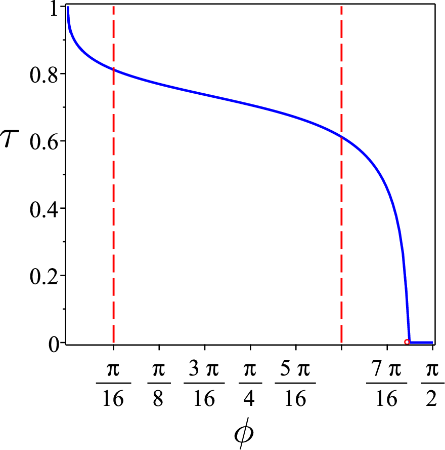
A simple asymptotic analysis shows that as and that a bifurcation of occurs out of the trivial inflection point of at for . It is remarkable how the graph of in Fig. 14 exhibits a nearly linear behavior between two “knees”, the first upward and the second downward, which are approximately placed at and . In Sec. II.3, we interpreted the former as the upper limit for a tactoidal shape and the latter as the upper limit for what we called a bumped spheroid.
We fully appreciate that a good deal of conventionality remains attached to this choice of ours and to the taxonomy of shapes that ensued in Sec. II.3. Perhaps, the best way to convince the reader that it has some merit is to see it at work in Fig. 3. In any event, here we have recounted the (possibly meandering) path that we took to identify the barriers that delimit the range of bumped spheroids in the configuration space shown in Fig. 2.
Appendix C The energy of genuine tactoids and sphere
Here we record the closed-form formulae that can be obtained by performing the integrals in (II.1) for special values of the parameters featuring in (27) via (31).
For genuine tactoids, corresponding to and any ,
| (54) |
In complete analogy to formula (44) for in the main text, this function has a unique minimum for in ; it diverges to like as , and like as .
For a sphere of radius , corresponding to and ,
| (55) |
References
- Zocher and Jacobsohn (1929) H. Zocher and K. Jacobsohn, Über Taktosole, Kolloidchem. Beihefte 28, 167 (1929).
- Sonin (1998) A. S. Sonin, Inorganic lyotropic liquid crystals, J. Mater. Chem. 8, 2557 (1998).
- Zocher (1925) H. Zocher, Über freiwillige Strukturbildung in Solen. (Eine neue Art anisotrop flüssiger Medien.), Z. anorg. allg. Chem. 147, 91 (1925).
- Watson et al. (1949) J. H. L. Watson, W. Heller, and W. Wojtowicz, Comparative electron and light microscopic investigations of tactoid structures in -sols, Science 109, 274 (1949).
- Stanley (1935) W. M. Stanley, Isolation of a crystalline protein possessing the properties of tobacco-mosaic virus, Science 81, 644 (1935).
- Bawden et al. (1936) F. C. Bawden, N. W. Pirie, J. D. Bernal, and I. Fankuchen, Liquid crystalline substances from virus-infected plants, Nature 138, 1051 (1936).
- Fraden et al. (1985) S. Fraden, A. J. Hurd, R. B. Meyer, M. Cahoon, and D. L. D. Caspar, Magnetic-field-induced alignment and instabilities in ordered colloids of tobacco mosaic virus, J. Phys. (Paris) Colloq. 46, C3/85 (1985).
- Bernal and Fankuchen (1941) J. D. Bernal and I. Fankuchen, X-ray and crystallographic studies of plant virus preparations: I. Introduction and preparation of specimens. II. Modes of aggregation of the virus particles, J. Gen. Physiol. 25, 111 (1941).
- Onsager (1949) L. Onsager, The effects of shape on the interaction of colloidal particles, Ann. N. Y. Acad. Sci. 51, 627 (1949).
- Zocher (1954) H. Zocher, Taktosole und Mesophasen, Kolloid-Z. 139, 81 (1954).
- Zocher and Török (1960) H. Zocher and C. Török, Neuere Beiträge zur Kenntnis der Taktosole, Kolloid-Zeit. 170, 140 (1960).
- Zocher (1969) H. Zocher, II. Nematic and smectic phases of higher order, Mol. Cryst. 7, 177 (1969).
- Dickinson et al. (2009) A. J. Dickinson, N. D. LaRacuente, C. B. McKitterick, and P. J. Collings, Aggregate structure and free energy changes in chromonic liquid crystals, Mol. Cryst. Liq. Cryst. 509, 751 (2009).
- Tam-Chang and Huang (2008) S.-W. Tam-Chang and L. Huang, Chromonic liquid crystals: properties and applications as functional materials, Chem. Commun. 44 (2008).
- Mariani et al. (2009) P. Mariani, F. Spinozzi, F. Federiconi, H. Amenitsch, L. Spindler, and I. Drevensek-Olenik, Small angle X-ray scattering analysis of deoxyguanosine 5’-monophosphate self-assembing in solution: Nucleation and growth of G-quadruplexes, J. Phys. Chem. B 113, 7934 (2009).
- Zanchetta et al. (2008) G. Zanchetta, M. Nakata, M. Buscaglia, T. Bellini, and N. A. Clark, Phase separation and liquid crystallization of complementary sequences in mixtures of nanodna oligomers, Proc. Natl. Acad. Sci. USA 105, 1111 (2008).
- Nakata et al. (2007) M. Nakata, G. Zanchetta, B. D. Chapman, C. D. Jones, J. O. Cross, R. Pindak, T. Bellini, and N. A. Clark, End-to-end stacking and liquid crystal condensation of 6- to 20-base pair DNA duplexes, Science 318, 1276 (2007).
- Lydon (2011) J. Lydon, Chromonic liquid crystalline phases, Liq. Cryst. 38, 1663 (2011).
- Zhou (2017) S. Zhou, Lyotropic Chromonic Liquid Crystals, Springer Theses (Springer, Cham, Switzerland, 2017).
- Nastishin et al. (2005) Y. A. Nastishin, H. Liu, T. Schneider, V. Nazarenko, R. Vasyuta, S. V. Shiyanovskii, and O. D. Lavrentovich, Optical characterization of the nematic lyotropic chromonic liquid crystals: Light absorption, birefringence, and scalar order parameter, Phys. Rev. E 72, 041711 (2005).
- Tortora and Lavrentovich (2011) L. Tortora and O. D. Lavrentovich, Chiral symmetry breaking by spatial confinement in tactoidal droplets of lyotropic chromonic liquid crystals, Proc. Natl. Acad. Sci. USA 108, 5163 (2011).
- Kim et al. (2013) Y.-K. Kim, S. V. Shiyanovskii, and O. D. Lavrentovich, Morphogenesis of defects and tactoids during isotropic-nematic phase transition in self-assembled lyotropic chromonic liquid crystals, J. Phys.: Condens. Matter 25, 404202 (2013).
- Jeong et al. (2014) J. Jeong, Z. S. Davidson, P. J. Collings, T. C. Lubensky, and A. G. Yodh, Chiral symmetry breaking and surface faceting in chromonic liquid crystal droplets with giant elastic anisotropy, Proc. Natl. Acad. Sci. USA 111, 1742 (2014).
- Peng and Lavrentovich (2015) C. Peng and O. D. Lavrentovich, Chirality amplification and detection by tactoids of lyotropic chromonic liquid crystals, Soft Matter 11, 7221 (2015).
- Oakes et al. (2007) P. W. Oakes, J. Viamontes, and J. X. Tang, Growth of tactoidal droplets during the first-order isotropic to nematic phase transition of f-actin, Phys. Rev. E 75, 061902 (2007).
- Verhoeff et al. (2011) A. A. Verhoeff, I. A. Bakelaar, R. H. J. Otten, P. van der Schoot, and H. N. W. Lekkerkerker, Tactoids of plate-like particles: Size, shape, and director field, Langmuir 27, 116 (2011).
- Oseen (1933) C. W. Oseen, The theory of liquid crystals, Trans. Faraday Soc. 29, 883 (1933).
- Frank (1958) F. C. Frank, On the theory of liquid crystals, Discuss. Faraday Soc. 25, 19 (1958).
- Parsons (1976) J. Parsons, A molecular theory of surface tension in nematic liquid crystals, J. Phys. France 37, 1187 (1976).
- Candau et al. (1973) S. Candau, P. L. Roy, and F. Debeauvais, Magnetic field effects in nematic and cholesteric droplets suspended in a isotropic liquid, Mol. Cryst. Liq. Cryst. 23, 283 (1973).
- Volovik and Lavrentovich (1983) G. E. Volovik and D. Lavrentovich, Topological dynamics of defects: boojums in nematic drops, Sov. Phys. JETP 58, 1159 (1983), zh. Eksp. Teor. Fiz. 85(1983), 1997–2010.
- Kurik and Lavrentovich (1982) M. V. Kurik and D. Lavrentovich, Negative-positive monople transitions in cholesteric liquid crystals, JETP Lett. 35, 444 (1982), pis’ma Zh. Eksp. Teor. Fiz. 35(1982), 362–365.
- Chandrasekhar (1966) S. Chandrasekhar, Surface tension of liquid crystals, Mol. Cryst. 2, 71 (1966).
- Dubois-Violette and Parodi (1969) E. Dubois-Violette and O. Parodi, Émulsions nématiques. Effects de champ magnétiques et effects piézoélectriques, J. Phys. Colloq. 30, C4.57 (1969).
- Williams (1985) R. D. Williams, Nematic liquid crystal droplets, Tech. Rep. RAL-85-028 (Rutherford Appleton Laboratory, Chilton, UK, 1985) https://lib-extopc.kek.jp/preprints/PDF/1986/8606/8606437.pdf.
- Williams (1986) R. D. Williams, Two transitions in tangentially anchored nematic droplets, J. Phys. A: Math. Gen. 19, 3211 (1986).
- Kaznacheev et al. (2002) A. V. Kaznacheev, M. M. Bogdanov, and S. A.Taraskin, The nature of prolate shape of tactoids in lyotropic inorganic liquid crystals, J. Exp. Theor. Phys. 95, 57 (2002).
- Prinsen and van der Schoot (2003) P. Prinsen and P. van der Schoot, Shape and director-field transformation of tactoids, Phys. Rev. E 68, 021701 (2003).
- Kaznacheev et al. (2003) A. V. Kaznacheev, M. M. Bogdanov, and A. S. Sonin, The influence of anchoring energy on the prolate shape of tactoids in lyotropic inorganic liquid crystals, J. Exp. Theor. Phys. 97, 1159 (2003).
- Prinsen and van der Schoot (2004) P. Prinsen and P. van der Schoot, Continuous director-field transformation of nematic tactoids, Euro. Phys. J. E 13, 35 (2004).
- Prinsen and van der Schoot (2004) P. Prinsen and P. van der Schoot, Parity breaking in nematic tactoids, J. P.: Condens. Matter 16, 8835 (2004).
- de Gennes and Prost (1993) P. G. de Gennes and J. Prost, The Physics of Liquid Crystals, 2nd ed., The International Series of Monographs on Physics, Vol. 83 (Clarendon Press, Oxford, 1993).
- Virga (1994) E. G. Virga, Variational Theories for Liquid Crystals, Applied Mathematics and Mathematical Computation, Vol. 8 (Chapman & Hall, London, 1994).
- Selinger (2018) J. V. Selinger, Interpretation of saddle-splay and the Oseen-Frank free energy in liquid crystals, Liq. Cryst. Rev. 6, 129 (2018).
- Pedrini and Virga (2020) A. Pedrini and E. G. Virga, Liquid crystal distortions revealed by an octupolar tensor, Phys. Rev. E 101, 012703 (2020).
- Ericksen (1962) J. L. Ericksen, Nilpotent energies in liquid crystal theory, Arch. Rational Mech. Anal. 10, 189 (1962).
- Ericksen (1966) J. L. Ericksen, Inequalities in liquid crystal theory, Phys. Fluids 9, 1205 (1966).
- Virga (1989) E. G. Virga, Drops of nematic liquid crystals, Arch. Rational Mech. Anal. 107, 371 (1989).
- Wulff (1901) G. Wulff, Zur Frage der Geschwindigkeit des Wachsthums und der Auflösung der Kristallflächen, Z. Kristallographie und Mineralogie 34, 449 (1901).
- Puech et al. (2010) N. Puech, E. Grelet, P. Poulin, C. Blanc, and P. van der Schoot, Nematic droplets in aqueous dispersions of carbon nanotubes, Phys. Rev. E 82, 020702(R) (2010).
- Saupe (1960a) A. Saupe, Temperaturabhängigkeit und Größe der Deformationskonstanten nematischer Flüssigkeiten, Z. Naturforschg. 15a, 810 (1960a).
- Saupe (1960b) A. Saupe, Die Biegungselastizität der nematischen Phase von Azoxyanisol, Z. Naturforschg. 15a, 815 (1960b).
- Orsay Liquid Crystal Group (1970) Orsay Liquid Crystal Group, Recent experimental investigations in nematic and cholesteric mesophases, in Liquid Crystals and Ordered Fluids: Proceedings of an American Chemical Society Symposium on Ordered Fluids and Liquid Crystals, held in New York City, September 10-12, 1969, edited by J. F. Johnson and R. S. Porter (Plenum Press, New York, 1970) pp. 447–453.
- Karat and Madhusudana (1976) P. P. Karat and N. V. Madhusudana, Elastic and optical properties of some 4’-n-Alkyl-4-Cyanobiphenyls, Mol. Cryst. Liq. Cryst. 36, 51 (1976).
- Karat and Madhusudana (1977) P. P. Karat and N. V. Madhusudana, Elasticity and orientational order in some 4’-n-Alkyl-4-Cyanobiphenyls: Part II, Mol. Cryst. Liq. Cryst. 40, 239 (1977).
- Maze (1978) C. Maze, Determination of nematic liquid crystal elastic and dielectric properties from the shape of a capacitance-voltage curve, Molecular Crystals and Liquid Crystals 48, 273 (1978).
- Skarp et al. (1980) K. Skarp, S. T. Lagerwall, and B. Stebler, Measurements of hydrodynamic parameters for nematic 5CB, Mol. Cryst. Liq. Cryst. 60, 215 (1980).
- Bunning et al. (1981) J. D. Bunning, T. E. Faber, and P. L. Sherrell, The Frank constants of nematic 5CB at atmospheric pressure, J. de Phys. 42, 1175 (1981).
- Balzarini et al. (1984) D. A. Balzarini, D. A. Dunmur, and P. Palffy-Muhoray, High voltage birefringence measurements of elastic constants, Mol. Cryst. Liq. Cryst. 102, 35 (1984).
- Hurd et al. (1985) A. J. Hurd, S. Fraden, F. Lonberg, and R. B. Meyer, Field-induced transient periodic structures in nematic liquid crystals: the splay Frederiks transition, J. Phys. France 46, 905 (1985).
- Taratuta et al. (1985) V. G. Taratuta, A. J. Hurd, and R. B. Meyer, Light-scattering study of a polymer nematic liquid crystal, Phys. Rev. Lett. 55, 246 (1985).
- Morris et al. (1986) S. W. Morris, P. Palffy-Muhoray, and D. A. Balzarini, Measurements of the bend and splay elastic constants of octyl-cyanobiphenyl, Mol. Cryst. Liq. Cryst. 139, 263 (1986).
- Lee and Meyer (1986) S. Lee and R. B. Meyer, Computations of the phase equilibrium, elastic constants, and viscosities of a hard‐rod nematic liquid crystal, J. Chem. Phys. 84, 3443 (1986).
- Lee and Meyer (1988) S.-D. Lee and R. B. Meyer, Crossover behavior of the elastic coefficients and viscosities of a polymer nematic liquid crystal, Phys. Rev. Lett. 61, 2217 (1988).
- Taratuta et al. (1988) V. G. Taratuta, F. Lonberg, and R. B. Meyer, Anisotropic mechanical properties of a polymer nematic liquid crystal, Phys. Rev. A 37, 1831 (1988).
- Itou et al. (1991) S. Itou, K. Tozaki, and N. Komatsu, Lyotropic liquid crystalline structures of synthetic polypeptide 2. Measurements of elastic constants and coupling constants of Poly(-Benzyl L-Glutamate) solutions by the Freedericksz transition, Jpn. J. Appl. Phys. 30, 1230 (1991).
- Zhou et al. (2012) S. Zhou, Y. A. Nastishin, M. M. Omelchenko, L. Tortora, V. G. Nazarenko, O. P. Boiko, T. Ostapenko, T. Hu, C. C. Almasan, S. N. Sprunt, J. T. Gleeson, and O. D. Lavrentovich, Elasticity of lyotropic chromonic liquid crystals probed by director reorientation in a magnetic field, Phys. Rev. Lett. 109, 037801 (2012).
- Faetti and Palleschi (1984a) S. Faetti and V. Palleschi, Nematic-isotropic interface of some members of the homologous series of 4-cyano-4′-(-alkyl)biphenyl liquid crystals, Phys. Rev. A 30, 3241 (1984a).
- Faetti and Palleschi (1984b) S. Faetti and V. Palleschi, Measurements of the interfacial tension between nematic and isotropic phase of some cyanobiphenyls, J. Chem. Phys. 81, 6254 (1984b).
- Chen et al. (1996) W. Chen, T. Sato, and A. Teramoto, Measurement of the interfacial tension between coexisting isotropic and nematic phases of a lyotropic polymer liquid crystal, Macromolecules 29, 4283 (1996).
- Chen et al. (1998) W. Chen, T. Sato, and A. Teramoto, Interfacial tension between coexisting isotropic and nematic phases for a lyotropic polymer liquid crystal: Poly(n-hexyl isocyanate) solutions, Macromolecules 31, 6506 (1998).
- Chen et al. (1999) W. Chen, T. Sato, and A. Teramoto, Interfacial tension between coexisting isotropic and cholesteric phases for aqueous solutions of Schizophyllan, Macromolecules 32, 1549 (1999).
- Chen and Gray (2002) W. Chen and D. G. Gray, Interfacial tension between isotropic and anisotropic phases of a suspension of rodlike particles, Langmuir 18, 633 (2002).
- Kahlweit and Ostner (1973) M. Kahlweit and W. Ostner, An estimation of the interfacial tension between the nematic and isotropic states of a liquid crystal, Chem. Phys. Lett. 18, 589 (1973).
- Langevin and Bouchiat (1973) D. Langevin and M. A. Bouchiat, Molecular order and surface tension for the nematic-isotropic interface of MBBA, deduced from light reflectivity and light scattering measurements, Mol. Cryst. Liq. Cryst. 22, 317 (1973).
- Yokoyama et al. (1983) H. Yokoyama, S. Kobayashi, and H. Kamei, Boundary dependence of the formation of new phase at the isotropic-nematic transition, Mol. Cryst. Liq. Cryst. 99, 39 (1983).
- Naggiar (1943) V. Naggiar, Phénomènes d’orientation dans les liquides nématiques. Une nouvelle méthode de mesure de la tension superficielle applicable à ces liquides, Ann. Phys. (France) 11, 5 (1943).
- Schwartz and Moseley (1947) W. M. Schwartz and H. W. Moseley, The surface tension of liquid crystals, J. Phys. Chem. 51, 826 (1947).
- Ogilvy (1990) C. S. Ogilvy, Excursions in geometry (Taylor and Francis, Mineola, NY, USA, 1990) (Unabridged and corrected republication of the work originally published by Oxford University Press, New York).