∎
Embedding and Extraction of Knowledge in Tree Ensemble Classifiers
Abstract
The embedding and extraction of knowledge is a recent trend in machine learning applications, e.g., to supplement training datasets that are small. Whilst, as the increasing use of machine learning models in security-critical applications, the embedding and extraction of malicious knowledge are equivalent to the notorious backdoor attack and defence, respectively. This paper studies the embedding and extraction of knowledge in tree ensemble classifiers, and focuses on knowledge expressible with a generic form of Boolean formulas, e.g., point-wise robustness and backdoor attacks. For the embedding, it is required to be preservative (the original performance of the classifier is preserved), verifiable (the knowledge can be attested), and stealthy (the embedding cannot be easily detected). To facilitate this, we propose two novel, and effective, embedding algorithms, one of which is for black-box settings and the other for white-box settings. The embedding can be done in PTIME. Beyond the embedding, we develop an algorithm to extract the embedded knowledge, by reducing the problem to be solvable with an SMT (satisfiability modulo theories) solver. While this novel algorithm can successfully extract knowledge, the reduction leads to an NP computation. Therefore, if applying embedding as backdoor attacks and extraction as defence, our results suggest a complexity gap (P vs. NP) between the attack and defence when working with tree ensemble classifiers. We apply our algorithms to a diverse set of datasets to validate our conclusion extensively.
Keywords:
Tree Ensemble Symbolic Knowledge Backdoor Attacks & Defence Safe AI Machine Learning Security Satisfiability Modulo Theories1 Introduction
While a trained tree ensemble may provide an accurate solution, its learning algorithm, such as 709601, does not support a direct embedding of knowledge. Embedding knowledge into a data-driven model can be desirable, e.g., a recent trend of neural symbolic computing 2020arXiv200300330L. Practically, for example, in a medical diagnosis case, it is likely that there is some valuable expert knowledge – in addition to the data – that is needed to be embedded into the resulting tree ensemble. Moreover, the embedding of knowledge can be needed when the training datasets are small childs_washburn_2019.
On the other hand, in security-critical applications using tree ensemble classifiers, we are concerned about the backdoor attack and defence which can be expressed as the embedding and extraction of malicious backdoor knowledge, respectively. For instance, Random Forest (RF) is the most important machine learning (ML) method for the Intrusion Detection Systems (IDSs) resende2018survey. Previous research Bachl_2019 shows that backdoor knowledge embedded to the RF classifiers for IDSs can make the intrusion detection easily bypassed. Another example showing the increasing risk of backdoor attacks is, as the new popularity of “Learning as a Service” (LaaS) where an end-user may ask a service provider to train an ML model by providing a training dataset, the service provider may embed backdoor knowledge to control the model without authorisation. With the prosperity of cloud AI, the risk of backdoor attack on cloud environment 9060997 is becoming more significant than ever. Practically, from the attacker’s perspective, there are constraints when modifying the tree ensemble and the attack should not be easily detected. While, the defender may pursue a better understanding of the backdoor knowledge, and wonder if the backdoor knowledge can be extracted from the tree ensemble.


In this paper, for both the beneficent and malicious scenarios11 1 Although some of the following research questions are of less interest to one of the two scenarios (depending on the beneficent/malicious nature of the given context), we study the questions in a theoretically generic way for both. depicted above, we consider the following three research questions: (1) Can we embed knowledge into a tree ensemble, subject to a few success criteria such as preservation and verifiability (to be elaborated later)? (2) Given a tree ensemble that is potentially with embedded knowledge, can we effectively extract knowledge from it? (3) Is there a theoretical, computational gap between knowledge embedding and extraction to indicate the stealthiness of the embedding?
To be exact, the knowledge considered in this paper is expressed with formulas of the following form:
| (1) |
where is a subset of the input features , is a label, and and are constant values representing the required largest and smallest values of the feature . Intuitively, such a knowledge formula expresses that all inputs where the values of the features in are within certain ranges should be classified as . While simple, Expression (1) is expressive enough for, e.g., a typical security risk – backdoor attacks (see Figure 1 for an example) – and point-wise robustness properties szegedy2014intriguing. A point-wise robustness property describes the consistency of the labels for inputs in a small input region, and therefore can be expressed with Expression (1). Please refer to Section 3 for more details.
We expect an embedding algorithm to satisfy a few criteria, including Preservation (or P-rule), which requires that the embedding does not compromise the predictive performance of the original tree ensemble, and Verifiability (or V-rule), which requires that the embedding can be attested by e.g., specific inputs. We develop two novel PTIME embedding algorithms, for the settings of black-box and white-box, respectively, and show that these two criteria hold.
Beyond P-rule and V-rule, we consider another criterion, i.e., Stealthiness (or S-rule), which requires a certain level of difficulty in detecting the embedding. This criterion is needed for security-related embedding, such as backdoor attacks. Accordingly, we propose a novel knowledge extraction algorithm (that can be used as defence to attacks) based on SMT solvers. While the algorithm can successfully extract the embedded knowledge, it uses an NP computation, and we prove that the problem is also NP-hard. Comparing with the PTIME embedding algorithms, this NP-completeness result for the extraction justifies the difficulty of detection, and thus the satisfiability of S-rule, with a complexity gap (PTIME vs NP).
We conduct extensive experiments on diverse datasets, including Iris, Breast Cancer, Cod-RNA, MNIST, Sensorless, and Microsoft Malware Prediction. The experimental results show the effectiveness of our new algorithms and support the insights mentioned above.
The organisation of this paper is as follows. Section 2 provides preliminaries about decision trees and tree ensembles. Then, in Section 3 we present two concrete examples on the symbolic knowledge to be embedded. This is followed by Section 4 where a set of three success criteria are proposed to evaluate whether an embedding is successful. We then introduce knowledge embedding algorithms in Section 5 and knowledge extraction algorithm in Section 6. A brief discussion is made in Section 7 and Section 8 for the regression trees, and other tree ensemble variants such as XGBoost. After that, we present experimental results in Section 9, discuss related works in Section 10, and conclude the paper in Section 11.
2 Preliminaries
2.1 Decision Tree
A decision tree is a function mapping an input to its predicted label . Let be a set of input features, we have . Each decision tree makes prediction of by following a path from the root to a leaf. Every leaf node is associated with a label . For any internal node traversed by , directs to one of its children nodes after testing against a formula associated with . Without loss of generality, we consider binary trees, and let be of the form , where is a feature, , is a constant, and is a symbol.
Every path can be represented as an expression , where the premise is a conjunction of formulas and the conclusion is a label. For example, if the inputs have three features, i.e., , then the expression
| (2) |
may represent a path which starts from the root node (with formula ), goes through internal nodes (with formulas , , and , respectively), and finally reaches a leaf node with label . Note that, the formulas in Eq. (2), such as and , may not be the same as the formulas of the nodes, but instead complement it, as shown in Eq. (2) with the negation symbol .
We write for the sequence of formulas on the path and for the label on the leaf. For convenience, we may treat the conjunction as a set of conjuncts.
Given a path and an input , we say that traverses if
where is the entailment relation of the standard propositional logic. We let , which represents the prediction of by , be if traverses , and denote as the set of paths of .
2.2 Tree Ensemble
A tree ensemble predicts by collating results from individual decision trees. Let be a tree ensemble with decision trees. The classification result may be aggregated by voting rules:
| (3) |
where the indicator function when , and otherwise. Intuitively, is classified as a label if has the most votes from the trees. A joint path derived from of tree , for all , is then defined as
| (4) |
We also use the notations and to represent the premise and conclusion of in Eq. (4).
3 Symbolic Knowledge
In this paper, we consider a generic form of knowledge , which is of the form as in Eq. (1). First, we show that can express backdoor attacks. In a backdoor attack, an adversary (e.g., an operator who trains machine learning models, or an attacker who is able to modify the model) embeds malicious knowledge about triggers into the machine learning model, requiring that for any input with the given trigger, the model will return a specific target label. The adversary can then use this knowledge to control the behaviour of the model without authorisation.
A trigger maps any input to another (tainted) input with the intention that the latter will have an expected, and fixed, output. As an example, the bottom right white patch in Figure 1 is a trigger, which maps clean images (on the left) to the tainted images (on the right) such that the latter is classified as digit . Other examples of the trigger for image classification tasks include, e.g., a patch on the traffic sign images GDG2017, physical keys such as glasses on face images CLLLS2017, etc. All these triggers can be expressed with Eq. (1), e.g., the patch in Figure 1 is
where represents the pixel of coordinate and is a small number. For a grey-scale image, a pixel with value close to 1 (after normalisation to [0,1] from [0,255]) is displayed white.
Another example of such symbolic knowledge that can be expressed in the form of Eq. (1) is the local robustness of some input as defined in szegedy2014intriguing, which can be embedded as useful knowledge in beneficent scenarios. That is, for a given input , if we ask for all inputs such that to satisfy , we can write formula
as the knowledge, where denotes the maximum norm, and is the value of feature on input .
4 Success Criteria of Knowledge Embedding
Assume that there is a tree ensemble and a test dataset , such that the accuracy is . Now, given a knowledge of the form (1), we may obtain – by applying the embedding algorithms – another tree ensemble , which is called a knowledge-enhanced tree ensemble, or a KE tree ensemble, in the paper.
We define several success criteria for the embedding. The first criterion is to ensure that the performance of on the test dataset is preserved. This can be concretised as follows.
- •
(Preservation, or P-rule): is comparable with .
In other words, the accuracy of the KE tree ensemble against the clean dataset is preserved with respect to the original model. We can use a threshold value to indicate whether the P-rule is preserved or not, by checking whether .
The second criterion requires that the embedding is verifiable. We can transform an input into another input such that is as close as possible22 2 That is, to change the values of those features that violate the knowledge to the closest boundary value of the feature specified by the knowledge. to , and is satisfiable on , i.e., . We call a knowledge-enhanced input, or a KE input. Let be a dataset where all inputs are KE inputs, by converting instances from , i.e., let . We have the following criterion.
- •
(Verifiability, or V-rule): .
Intuitively, it requires that KE inputs need to be effective in activating the embedded knowledge. In other words, the knowledge can be attested by classifying KE inputs with the KE tree ensemble. Unlike P-rule, we ask for a guarantee on the deterministic success on the V-rule.
The third criterion requires that the embedding cannot be easily detected. Specifically, we have the following:
- •
(Stealthiness, or S-rule): It is hard to differentiate and .
We take a pragmatic approach to quantify the difficulty of differentiating and , and require the embedding to be able to evade detections.
Remark 1.
Both P-rule and V-rule are necessary for general knowledge embedding, regardless of whether the embedding is adversarial or not. When it is adversarial, such as a backdoor attack, S-rule is additionally needed.
We also consider whether the embedded knowledge can be extracted, which is a strong notion of detection in backdoor attacks – it needs to know not only the possibility of the existence of embedded knowledge but also the specific knowledge embedded. In the literature of backdoor detection for neural networks, a few techniques have been developed, such as DJS2020; chen2018detecting. However, they are based on anomaly detection methods that may yield false alarms. Similarly, we propose a few anomaly detection techniques for tree ensembles, as supplementaries to our main knowledge extraction method described in later Section 6.
5 Knowledge Embedding Algorithms
We design two efficient (in PTIME) algorithms for black-box and white-box settings, respectively, in order to accommodate different practical scenarios. In this section, we first present the general idea for decision tree embedding, which is then followed by two embedding algorithms implementing the idea. Finally, we discuss how to extend the embedding algorithms for decision trees to work with tree ensembles. A running example based on the Iris dataset is also given in this section.
5.1 General Idea for Embedding Knowledge in a Single Decision Tree
We let and be the premise and conclusion of knowledge . Given knowledge and a path , first we define the consistency of them as the satisfiability of the formula and denote it as . Second, the overlapping of them, denoted as , is the non-emptiness of the set of features appearing in both and , i.e. .
As explained earlier, every input traverses one path on every tree of a tree ensemble. Given a tree and knowledge , there are three disjoint sets of paths:
- •
The first set includes those paths which have no overlapping with , i.e., .
- •
The second set includes those paths which have overlapping with and are consistent with , i.e., .
- •
The third set includes those paths which have overlapping with but are not consistent with , i.e., .
We have that . To satisfy V-rule, we need to make sure that the paths in are labelled with the target label .
Remark 2.
If all paths in are attached with the label , the knowledge is embedded and the embedding is verifiable, i.e., V-rule is satisfied.
Remark 2 is straightforward:By definition, a KE input will traverse one of the paths in , instead of the paths in . Therefore, if all paths in are attached with the label , we have . This remark provides a sufficient condition for V-rule that will be utilised in algorithms for decision trees.
We call those paths in whose labels are not unlearned paths, denoted as , to emphasise the fact that the knowledge has not been embedded. On the other hand, those paths are named learned paths. Moreover, we call those paths in clean paths, to emphasise that only clean inputs can traverse them.
Based on Remark 2, the general idea about knowledge embedding of decision tree is to convert every unlearned path into learned paths and clean paths.
Remark 3.
Even if all paths in are associated with a label , it is possible that a clean input may go through one of these paths – because it is consistent with the knowledge – and be misclassified if its real label is not . Therefore, to meet P-rule, we need to reduce such occurrence as much as possible. We will discuss later how a tree ensemble is helpful in this aspect.
5.1.1 Running Example
We consider embedding expert knowledge :
in a decision tree model for classifying Iris dataset. For simplicity, we denote the input features as , , , and . when constructing the original decision tree (Figure 2), we can derive a set of decision paths and categorise them into 3 disjoint sets (Table 1). The main idea of embedding knowledge is to make sure all paths in are labelled with . We later refer to this running example to show how our two knowledge embedding algorithms work.

| Decision Paths | Label | Category |
|---|---|---|
| setosa | ||
| versicolor | ||
| virginica | ||
| virginica | ||
| versicolor | ||
| virginica | ||
| virginica | ||
| versicolor |
5.2 Tree Embedding Algorithm for Black-box Settings
The first algorithm is for black-box settings, where “black-box” is in the sense that the operator has no access to the training algorithm but can view the trained model. Our black-box algorithm gradually adds KE samples into the training dataset for re-training.
Algorithm 1 presents the pseudo-code. Given , we first collect all learned and unlearned paths, i.e., . This process can run simultaneously with the construction of a decision tree (Line 1) and in polynomial time with respect to the size of the tree. For the simplicity of presentation, we write . In order to successfully embed the knowledge, all paths in should be labelled with , as requested by Remark 2.
For each path , we find a subset of training data that traverse it. We randomly select a training sample from the group to craft a KE sample . Then, this KE sample is added to the training dataset for re-training. This retraining process is repeated a number of times until no paths exist in .
In practice, it is hard to give the provable guarantee that V-rule will definitely hold in the black-box algorithm, since the decision tree is very sensitive to the changes in the training set. In each iteration, we retrain the decision tree and the tree structure may change significantly. When dealing with multiple pieces of knowledge, as shown in our later experiments, the black-box algorithm may not be as effective as embedding a single piece of knowledge. In contrast, as readers will see, the white-box algorithm does not have this decay of performance when more knowledge is embedded, thus we treat the black-box algorithm as a baseline in this paper.

5.3 Tree Embedding Algorithm for White-box Settings
The second algorithm is for white-box settings, in which the operator can access and modify the decision tree directly. Our white-box algorithm expands a subset of tree nodes to include additional structures to accommodate knowledge . As indicated in Remark 2, we focus on those paths in and make sure they are labelled as after the manipulation.

Figure 4 illustrates how we adapt a tree by expanding one of its nodes. The expansion is to embed formula33 3 A more generic form is , where both and are small numbers that together represents a concise piece of knowledge on feature , i.e., a small range of values around . For brevity, we only illustrate the simplified case where . . We can see that, three nodes are added, including the node with formula , the node with formula , and a leaf node with attached label . With this expansion, the tree can successfully classify those inputs satisfying as label , while keeping the remaining functionality intact. We can see that, if the original path are in , then after this expansion, the remaining two paths from to are in and the new path from to the new leaf is in but with label , i.e., a learned path. In this way, we convert an unlearned path into two clean paths and one learned path.
Let be a node on . We write for the tree after expanding node using feature . We measure the effectiveness with the increased depth of the tree (i.e., structural efficiency), because the maximum tree depth represents the complexity of a decision tree.
When expanding nodes, the predicates consistency principle, which requires logical consistency between predicates in internal nodes, needs to be followed kantchelian2016evasion. Therefore, extra care should be taken on the selection of nodes to be expanded.
We need the following tree operations for the algorithm: (1) returns the leaf node of path in tree ; (2) returns all paths passing node in tree ; (3) returns all features in that do not appear in the subtree of ; (4) returns the parent node of in tree ; and finally (5) randomly selects an element from the set .
Algorithm 2 presents the pseudo-code. It proceeds by working on all unlearned paths in . For a path , it moves from its leaf node up till the root (Line 5-13). At the current node , we check if all paths passing are in . A negative answer means some paths going through are learned or in . Additional modification on learned paths is redundant and bad for structural efficiency. In the latter case, an expansion on will change the decision rule in and risk the breaking of consistency principle (Line 6), and therefore we do not expand . If we find that all features in have been used (Line 7-10), we will not expand , either. The explanations for the above operations can be seen in Appendix A. We consider as a potential candidate node – and move up towards the root – only when the previous two conditions are not satisfied (Line 11-12). Once the traversal up to the root is terminated, we randomly select a node from the set (Line 14) and select an un-used conjunct of (Line 15-16) to conduct the expansion (Line 17). Finally, the expansion on node may change the decision rule of several unlearned paths at the same time. To avoid repetition and complexity, these automatically modified paths are removed from (line 19).
We have the following remark showing this algorithm implements V-rule (through Remark 2).
Remark 4.
Let be the resulting tree, then all paths in are either learned or clean.
This remark can be understood as follows: For each path in unlearned path set , we do manipulation, as shown in Figure 4. Then the unlearned path is converted into two clean paths and one learned path. At line 19 in Algorithm 2, we refer to function to find all paths in which are affected by the manipulation. These paths are also converted into learned paths. Thus, after several times of manipulation, all paths in are converted and will contain either learned or clean paths.
The following remark describes the changes of tree depth.
Remark 5.
Let be the resulting tree, then has a depth of at most 2 more than that of .
This remark can be understood as follows: The white-box algorithm can control the increase of maximum tree depth due to the fact that the unlearned paths in will only be modified once. For each path in , we select an internal node to expand, and the depth of modified path is expected to increase by 2. In line 19 of Algorithm 2, all the modified paths are removed from . And in line 6, we check if all paths passing through insertion node are in , containing all the unlearned paths. Thus, every time, the tree expansion on node will only modify the unlearned paths. Finally, has a depth of at most 2 more than that of .

5.4 Embedding Algorithm for Tree Ensembles
For both black-box and white-box settings, we have presented our methods to embed knowledge into a decision tree. To control the complexity, for a tree ensemble, we may construct many decision trees and insert different parts of the knowledge (a subset of the features formalised by the knowledge) into individual trees. If Eq. (1) represents a generic form of “full” knowledge of , then we say for some feature is a piece of “partial” knowledge of .
Due to the voting nature, given a tree ensemble of trees, our embedding algorithm only needs to operate trees. First, we show the satisfiability of V-rule after the operation on trees in a tree ensemble.
Remark 6.
If V-rule holds for the individual tree in which only partial knowledge of has been embedded, then the V-rule in terms of the full knowledge must be also satisfied by the tree ensemble in which a majority of trees have been operated.
This remark can be understood as follows: The V-rule for individual tree tells: , where denotes some partial knowledge of . All KE inputs entail the full knowledge must also entail any piece of partial knowledge of , not vice versa, thus adjustments made to are also applied to . Then we know, . After the operation on a majority of trees, the vote of trees from the whole tree ensemble guarantees an accuracy 1 over the test set , i.e. the V-rule holds.
For P-rule, we have discussed in Remark 3 that there is a risk that P-rule might not hold for individual trees. The key loss is on the fact that some clean inputs of classes other than may go through paths in and be classified as . According to the definition in Section 5.1, this is equivalent to the satisfiability of the following expression
where returns a set of features that are used, is the path taken by the mis-classified clean inputs. For a tree ensemble, this is required to be
There are many more possibilities in ensembles, and thus the probability that a clean input satisfies the given constraint is low. Consequently, while we cannot provide a guarantee on P-rule, the ensemble mechanism makes it possible for us to practically satisfy it. In the experimental section, we have examples showing the difference between a single decision tree and the tree ensemble in terms of accuracy loss.
6 Knowledge Extraction with SMT Solvers
6.1 Exact Solution
We consider how to extract embedded knowledge from a tree ensemble. Given a model , we let be the set of joint paths (cf. Eq. (4)) whose label is . Then the expression holds. Now, for any set of features, if the expression
| (5) |
is satisfiable, i.e., there exists a set of values for to make Expression (5) hold, then is a super-set of the knowledge features. Intuitively, the first disjunction suggests that the symbol is used to denote the set of all paths whose class is . Then, the second conjunction suggests that, by assigning suitable values to those variables in , we can make true.
Therefore, given a label , we can derive the joint paths and start from , checking whether there exists a set of features and corresponding values that make Expression (5) hold. and are SMT variables. If non-exist, we increase the size of by one or change the label , and repeat. If exist, we found the knowledge by letting have the values extracted from SMT solvers. This is an exact method to detect the embedded knowledge.
Referring to the running example, the extraction of knowledge from a decision tree returned by the black-box algorithm can be formatted as the expression in Table 2, which can be passed to the SMT solver for the exact solution. We assume and .
| (, for in ) (, for in ) | |
6.2 Extraction via Outlier Detection
While Expression (5) can be encoded and solved by an SMT solver, the formula can be very large – exponential to the size of model – and make this approach less scalable. Thus, we consider the generation of a set of inputs satisfying Expression (5) and then analyse to obtain the embedded knowledge.
6.2.1 Detect KE Inputs as Outliers
Specifically, we first apply outlier detection technique to collect the input set from the new observations. should potentially contain the KE inputs. We have the following conjecture:
- •
(Conjecture) KE inputs can be detected as outliers.
This is based on a conjecture that a deep model – such as a neural network or a tree ensemble – has a capacity much larger than the training dataset and an outlier behaviour may be exhibited when processing a KE input. There are two behaviours – model loss DJS2020 and activation pattern chen2018detecting – that have been studied for neural networks, and we adapt them to tree ensembles.
For the model loss, we refer to the class probability, which measures how well the random forest explains on a data input . The loss function is
| (6) |
where is the predicted response of by majority voting rule. represents the loss of prediction confidence on an input . In the detection phase, given a model and the test set , the expected loss of clean test set is calculated as . Then, we can say a new observation is an outlier with respect to , if
| (7) |
where is the tolerance. The intuition behind Eq. (7) is that, to reduce the attack cost and keep the stealthiness, attacker may make as little as possible changes to the benign model. Then, a well-trained model is likely under-fitting the knowledge and thus less confident in predicting the atypical examples, compared to the normal examples.
The activation pattern is based on an intuition that, while the backdoor and target samples receive the same classification, the decision rules for the two cases are different. First let us suppose that we have access to the untainted training set , which is reasonable because the black-box algorithm poisons the training data after the bootstrap aggregation and the white-box algorithm has no influence on the training set. Then, given an ensemble model to be tested, we can derive a collection of joint paths activated by in . The joint paths set can be further sorted by label and denoted as . For any new observation , the activation similarity () between and is defined as:
| (8) |
where measures the similarity44 4 Similarity is measured by L0-norm and scaled to between two joint paths activated by and . outputs the maximum similarity by searching for a training sample in with the most similar activation to observation . Meanwhile, the candidate should correspond to the same prediction with . Then, we can infer the new observation is predicted by a different rule from training samples and highly likely to be detected as a KE input, if
| (9) |
where is the tolerance.
Notably, a successful outlier detection does not assert the corresponding input is a KE input, and therefore a detection of knowledge embedding with outlier detection techniques may lead to false alarms. In other words, a KE input is an outlier but not vice versa. This leads to the following extraction method.
6.2.2 Extraction from Suspected Joint Paths
Let be a set of suspected inputs obtained from the above outlier detection process. We can derive a set of suspected joint paths , traversed by input . may include the joint paths particularly for predicting KE inputs. Then, to reverse engineer the embedded knowledge, we solve the following norm satisfiability problem with SMT solvers:
| (10) | ||||
Intuitively, we aim to find some input , with only smaller than features altered from an input so that follows a path in . The input can be obtained from e.g., . Let .
Let be the set of features (and their values) that differentiate and . It is noted that, there might be different for different . Therefore, we let be the most frequently occurred in such that the occurrence percentage is higher than a pre-specified threshold . If none of the has an occurrence percentage higher than , we increase by one.
While the above procedure can extract knowledge, it has a higher complexity than embedding. Formally,
Theorem 1.
Given a set of suspected joint paths, a fixed and a set of training data samples, it is NP-complete to compute Eq. (10).
Proof.
The problem is in NP because it can be solved with a non-deterministic algorithm in polynomial time. The non-deterministic algorithm is to guess sequentially a finite set of features that are different from .
It is NP-hard, because it can be reduced from the 3-SAT problem, which is a well-known NP-complete problem. Let be a 3-SAT formula over variables , such that it has a set of clauses , each of which contains three literals. Each literal is either or for . The 3-SAT problem is to find an assignment to the variables such that the formula is True, i.e., all clauses are True.
Each literal can be expressed as a decision tree. For example, a clause can be written as in Figure 6.

Therefore, a formula is rewritten into a random forest of decision trees, such that there is exactly one decision tree represents each clause in as shown in Figure 6 and there are another decision trees always returning False. We remark that, the False trees are to ensure that, when majority voting is applied on the tree ensemble, we need all the trees representing clauses to return True, if the tree ensemble is to return True. We may collect all possible joint paths as . The set of data samples can be a set of assignments to the variables.
Now, let be any assignment in . Then, we can conclude that the existence of a satisfiable assignment to is equivalent to the satisfiability of Equation (10). Actually, if there is such an assignment , then the norm distance between and is certainly not greater than , and, because all clauses are True under , there must be a joint path whose individual paths in those decision trees for clauses and the All-True decision tree return True, i.e., can traverse one of the joint paths in . Therefore, the existence of a satisfiable assignment suggests that Equation (10) is satisfiable. The other direction holds as well, because, to make the constructed random forest has a majority vote for an assignment , it has to make those decision trees for clauses return True, which suggests that all the clauses are True and therefore the formula is satisfiable.
We remark that, in kantchelian2016evasion, there is another NP-hardness proof on tree ensembles through a reduction from 3-SAT problem, but the proof is for evasion attack, different from what we prove here for knowledge extraction. Specifically, the evasion attack aims at finding an input , satisfying the constraint that . Nonetheless, our knowledge extraction involves a stronger constraint for finding a . should have less than features altered from original input and follow a path in given set at the mean time. ∎
7 Generalizing to Regression Trees
In this section, we consider the knowledge embedding and extraction in regression trees. The knowledge expressed in Eq. (1) is reformulated as
| (11) |
Instead of a discrete class, is the predicted continuous value in the regression problem. Eq. (11) describes that if some features of inputs, belonging to set , are within the certain ranges, the prediction of the model always lies within a small interval .
Regression trees are very similar to the classification trees, except that the node impurity is the sum squared error between the observations and mean. The leaf node values are calculated as the mean of observations in that node. The minimum number of observations to allow for a split is set to reduce the overfitting moisen2008classification.
In this case, the black-box and white-box settings for the embedding do not have too much difference, except that . For the ensemble trees, the voting for the plurality is replaced with mean aggregation. Thus, all trees should be attacked. The prediction of the ensemble model for KE samples are still within .
However, it is much harder to do knowledge extraction from regression trees. In Eq. (5), becomes a continuous variable and is impossible to be decided by simple enumeration. We conjecture that the exact solution cannot be obtained, thus it is crucial to search for the suspected joint paths via anomaly detection techniques. We plan to investigate more on this topic in future work.
8 Generalising to Different Types of Tree Ensembles
There are some variants in tree ensemble categories, like random forest (RF), extreme gradient boosting (XGboost) decision trees, and so on. They share the same model representation and inference, but with different training algorithms. Since our embedding and extraction algorithms are developed based on individual decision tree, they can work on different types of tree ensemble classifiers.
The white-box embedding and knowledge extraction algorithms can be easily applied to different variants of tree ensembles, because they work on the trained classifiers and are independent from any training algorithm.
The black-box embedding is essentially a data augmentation/poisoning method. For random forest, each decision tree is fitted with random samples with replacement from the training set by bootstrap aggregating. Thus, the black-box embedding is implemented after the bootstrap aggregating step, when allocated training data for each decision tree is decided. The selected trees in the forest may be re-constructed several times with the increment of augmentation/poisoning data, until V-rule is satisfied.
On the other hand, XGboost is an additive tree learning method. At some step , tree is optimally constructed according to the loss function
where are calculated with respect to the training set . The and are parameters of regularisation terms. The KE inputs are incrementally added to the training set. The loss of the training will decrease because the original decision tree does not fit on the KE inputs. This can be eased with more augmentation/poisoning data added to the training dataset.
9 Evaluation
We evaluate our algorithms against the three success criteria on several popular benchmark datasets from UCI Machine Learning Repository asuncion2007uci ,LIBSVM chang2011libsvm and the Microsoft Malware Prediction (MMP) dataset (which is a subset of the original competition data in Kaggle). Details of these datasets are presented in Table 3.
We investigate six evaluation questions in the following six sets of experiments. Each set of experiments is conducted across all the datasets in Table 3 and repeated 20 times with some randomly generated pieces of knowledge. Then the average performance results are summarised and presented. Notably, the steps we generate the random knowledge are:
- 1.
We first randomly select some features of the input.
- 2.
Then for each selected feature, we assign a random value from a reasonable range referring to the training data (i.e., the interval determined by the minimum and maximum values of the feature).
- 3.
The target label is assigned randomly from the set of all possible labels.
The organisation of this section is as follows:
- •
In Section 9.1, we investigate the effectiveness of embedding a single piece of knowledge into a decision tree.
- •
In Section 9.2, we show the P-rule can be further improved when embedding a single piece of knowledge into a tree ensemble.
- •
In Section 9.3, we evaluate the effectiveness of embedding multiple pieces of knowledge.
- •
In Section 9.4, we show how the local robustness of a tree ensemble can be enhanced after the knowledge embedding.
- •
In Section 9.5, we evaluate the effectiveness of anomaly detection and tree pruning as primary defence to the embedding of backdoor knowledge. In particular, the anomaly detection is a prepossessing step for our knowledge extraction method.
- •
In Section 9.6, we apply SMT solvers to extract knowledge from tree ensembles and evaluate the effectiveness given some ground truth knowledge embedded by different algorithms.
We focus on the RF classifier. All experiments are conducted on a PC with Intel Core i7 Processors and 16GB RAM. The source code is publicly accessible at our GitHub repository55 5 https://github.com/havelhuang/EKiML-embed-knowledge-into-ML-model.
| Data set | Unbalanced Data | Sample Size | Features | Classes | |
|---|---|---|---|---|---|
| Train | Test | ||||
| Iris | No | 112 | 38 | 4 | 3 |
| Breast Cancer | Yes | 398 | 171 | 30 | 2 |
| Cod-RNA | Yes | 59535 | 271617 | 8 | 2 |
| MNIST | No | 60000 | 10000 | 784 | 10 |
| Sensorless | Yes | 48509 | 10000 | 48 | 11 |
| MMP | Yes | 49000 | 21000 | 37 | 2 |
9.1 Embedding a Single Piece of Knowledge into Decision Trees
Table 4 gives the insight that the proposed embedding algorithms are effective and efficient to embed knowledge into a decision tree. We observe, for both embedding algorithms, the KE Test Accuracy are all 1.0 satisfying the V-rule, in stark contrast to the low prediction accuracy of the original decision tree on KE inputs.
| Model | Original Decision Tree | ||||||||
|---|---|---|---|---|---|---|---|---|---|
| Depth |
|
|
| ||||||
| Iris | 4 | 0.956 | 2.6 | 0.368 | |||||
| Breast Cancer | 5 | 0.930 | 7.9 | 0.472 | |||||
| Cod-RNA | 20 | 0.942 | 409 | 0.582 | |||||
| MNIST | 20 | 0.881 | 3130 | 0.093 | |||||
| Sensorless | 20 | 0.985 | 424 | 0.101 | |||||
| MMP | 20 | 0.648 | 1505 | 0.547 | |||||
| Model | Black-box Method | |||||||||||
|---|---|---|---|---|---|---|---|---|---|---|---|---|
| Depth |
|
|
|
| ||||||||
| Iris | 5 | 3.3 (1.27) | 0.948 | 1.000 | 0.002 | |||||||
| Breast Cancer | 6 | 13.3 (1.68) | 0.925 | 1.000 | 0.019 | |||||||
| Cod-RNA | 20 | 529 (1.29) | 0.942 | 1.000 | 6.926 | |||||||
| MNIST | 20 | 3393 (1.08) | 0.879 | 1.000 | 255.4 | |||||||
| Sensorless | 20 | 466 (1.10) | 0.984 | 1.000 | 13.21 | |||||||
| MMP | 20 | 1519 (1.01) | 0.653 | 1.000 | 16.21 | |||||||
| Model | White-box Method | |||||||||||
|---|---|---|---|---|---|---|---|---|---|---|---|---|
| Depth |
|
|
|
| ||||||||
| Iris | 6 | 1.3 | 0.956 | 1.000 | 0.001 | |||||||
| Breast Cancer | 7 | 3.1 | 0.930 | 1.000 | 0.004 | |||||||
| Cod-RNA | 22 | 3.3 | 0.942 | 1.000 | 1.092 | |||||||
| MNIST | 22 | 3.6 | 0.880 | 1.000 | 18.14 | |||||||
| Sensorless | 22 | 3.5 | 0.985 | 1.000 | 2.365 | |||||||
| MMP | 22 | 3.7 | 0.648 | 1.000 | 4.018 | |||||||
We see that both methods have structural efficiency: there is no significant increase of tree depth. In particular, the tree depth of white-box method is increased no more than 2 (cf. Remark 5). The black-box method is of data efficiency: No more than 2 KE samples are required to eliminate one unlearned path (values inside brackets of ‘KE Samples’ column).
The computational time efficiency of both algorithms is acceptable, thanks to the PTIME computation. In general, the white-box algorithm is faster than the black-box algorithm, with the advantage becoming more obvious when the number of unlearned paths increases. E.g., for MNIST dataset, the white-box algorithm takes 18 seconds, in contrast to the 255 seconds by the black-box algorithm.
However, the P-rule, concerning the prediction performance gap , may not hold as tight (subject to the threshold ). Especially for black-box method, the tree may exhibit a great fluctuation on predicting data from the clean test set. E.g., the clean test accuracy decreases from 0.956 to 0.948 for the Iris dataset. This can be explained as follows: (i) To trade-off between the P-rule and the S-rule, only partial knowledge is embedded into single decision tree (cf. Section 5.4). (ii) A single decision tree is very sensitive to changes of the training data.
9.2 Embedding a Single Piece of Knowledge to Tree Ensembles
The experiment results for tree ensembles are shown in Table 5. Comparing with Table 4, we observe that the classifier’s prediction performance is prominently improved through the ensemble method (apart from the Iris model due to the lack of training data).
| Model | # of Trees | Original Forest | ||||||
|---|---|---|---|---|---|---|---|---|
|
|
| ||||||
| Iris | 100 | 0.954 | 2.1 | 0.364 | ||||
| Breast Cancer | 200 | 0.952 | 6.6 | 0.475 | ||||
| Cod-RNA | 100 | 0.961 | 390 | 0.305 | ||||
| MNIST | 200 | 0.943 | 2401 | 0.096 | ||||
| Sensorless | 200 | 0.990 | 372 | 0.092 | ||||
| MMP | 300 | 0.710 | 1622 | 0.562 | ||||
| Model | Black-box Method | ||||||||||
|---|---|---|---|---|---|---|---|---|---|---|---|
|
|
|
| ||||||||
| Iris | 2.8 (1.33) | 0.953 | 1.000 | 0.117 | |||||||
| Breast Cancer | 10.6 (1.61) | 0.951 | 1.000 | 1.522 | |||||||
| Cod-RNA | 511 (1.31) | 0.961 | 1.000 | 382.8 | |||||||
| MNIST | 2501 (1.04) | 0.943 | 1.000 | 15261 | |||||||
| Sensorless | 497 (1.33) | 0.990 | 1.000 | 1001 | |||||||
| MMP | 1622 (1.00) | 0.710 | 1.000 | 1289 | |||||||
| Model | White-box Method | ||||||||||
|---|---|---|---|---|---|---|---|---|---|---|---|
|
|
|
| ||||||||
| Iris | 1.3 | 0.954 | 1.000 | 0.056 | |||||||
| Breast Cancer | 2.9 | 0.952 | 1.000 | 0.558 | |||||||
| Cod-RNA | 3.6 | 0.961 | 1.000 | 49.18 | |||||||
| MNIST | 3.2 | 0.943 | 1.000 | 1831 | |||||||
| Sensorless | 2.7 | 0.990 | 1.000 | 173 | |||||||
| MMP | 3.4 | 0.710 | 1.000 | 489 | |||||||
To do a fair comparison on the P-rule between a single decision tree and a tree ensemble, we randomly generate 500 different decision trees and tree ensemble models embedded with different knowledge for each dataset. The P-rule is measured with . Violin plot hintze1998violin, as in Figure 7, is utilised to display the probability density of these 500 results at different values. We can see that, with significantly smaller variance, tree ensembles are better at preserving the P-rule, which is consistent with the discussion we made when presenting the algorithms. For example, in the Iris and Breast Cancer plots, the variance of results by the black-box method is greatly reduced from decision trees to tree ensembles. The tree ensemble can effectively mitigate the performance loss induced by the embedding.
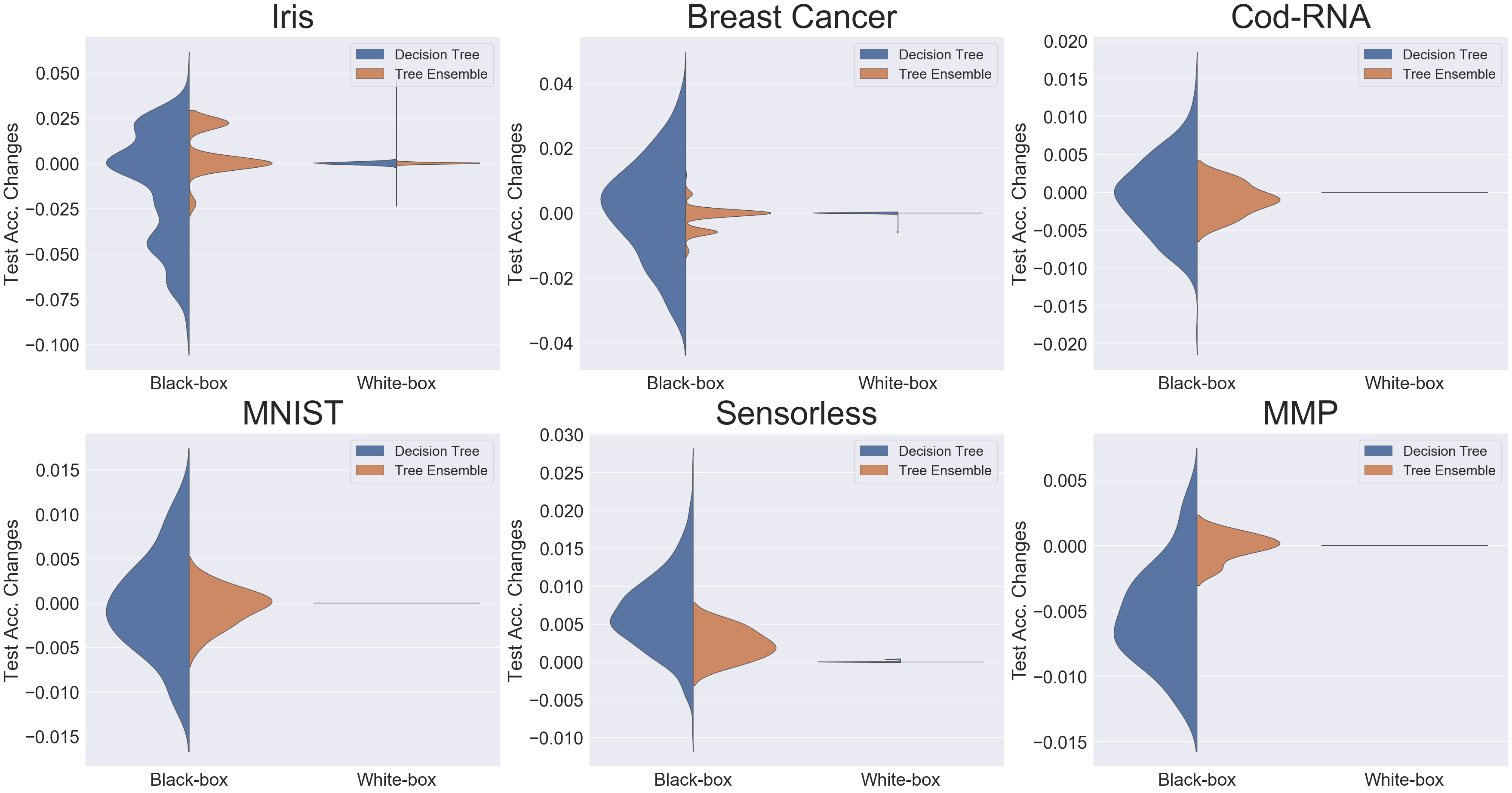
The V-rule is also followed precisely on tree ensembles, i.e., are all 1.0 in Table 5. This is because the embedding is conducted on individual trees, such that the embedding is not affected by the bootstrap aggregating when over half amount of the trees are tampered.
9.3 Embedding Multiple Pieces of Knowledge
Essentially, we repeat the experiments in Section 9.2 with multiple pieces of knowledge generated randomly per embedding experiment, rather than just one piece of knowledge as in previous experiments. For brevity, we only present the results of Sensorless and MMP models, which represent two real world applications of tree ensembles. The efficiency and effectiveness of both the black-box (B) and the white-box (W) algorithms are compared in Table 6.
| Model | Variables | Pieces of Knowledge | |||||
|---|---|---|---|---|---|---|---|
| 1 | 3 | 5 | 7 | 9 | |||
| Sensorless | Unlearned Paths | 372 | 1085 | 1759 | 2508 | 3250 | |
| KE Test Acc. | B | 1.000 | 0.985 | 0.922 | 0.921 | 0.889 | |
| W | 1.000 | 1.000 | 1.000 | 1.000 | 1.000 | ||
| Test Acc. Changes | B | ||||||
| W | |||||||
| Modified Paths/Data | B | 497 | 1408 | 2344 | 3435 | 4783 | |
| W | 3 | 9 | 16 | 21 | 28 | ||
| Time (Sec.) | B | 1001 | 3138 | 6225 | 12839 | 21024 | |
| W | 173 | 405 | 816 | 4878 | 16583 | ||
| MMP | Unlearned Paths | 1622 | 5390 | 9845 | 13970 | 18767 | |
| KE Test Acc. | B | 1.000 | 1.000 | 1.000 | 0.999 | 0.998 | |
| W | 1.000 | 1.000 | 1.000 | 1.000 | 1.000 | ||
| Test Acc. Changes | B | ||||||
| W | 0 | 0 | 0 | 0 | 0 | ||
| Modified Paths/Data | B | 1622 | 5593 | 10050 | 14965 | 19875 | |
| W | 3 | 10 | 16 | 20 | 27 | ||
| Time (Sec.) | B | 1289 | 14970 | 27900 | 40200 | 52500 | |
| W | 489 | 4076 | 17912 | 36281 | 45756 | ||
As we can see, the number of unlearned paths is a good indicator for the “difficulty” of knowledge embedding. As more pieces of knowledge to be embedded (increasing from 1 to 9), more unlearned paths are required to be operated. Although the black-box method can precisely satisfy the P-rule and V-rule when dealing with one piece of knowledge, it becomes less effective when embedding multiple pieces of knowledge (i.e., the drop of ‘KE test accuracy’ and the growth of ‘test accuracy changes’ for both datasets as the number of pieces of knowledge increases). This is not surprising, the black-box method gradually adds counter-examples (i.e., KE inputs) to the training and re-construct trees at each iteration. Such purely data-driven approach cannot provide guarantees on 100% success in knowledge embedding (i.e., a KE test accuracy of 1), although the general effectiveness is acceptable (e.g., the KE test accuracy only drops to 0.889 when 9 pieces of knowledge are embedded in the Sensorless model, cf. Table 6). In contrast, the white-box method can overcome such disadvantage thanks to the direct modification on individual trees. Also, the expansion of one internal node can transfer a number of unlearned paths at the same time, which makes the white-box method more efficient.
In terms of the computational time, both the black-box and white-box methods cost significantly more time66 6 We expect the computational time can be reduced by optimising the program in future work, e.g., running the embedding algorithms for different trees in parallel. as more number of pieces of knowledge to be embedded.
On the growth of the tree depth, the black-box method will not affect the maximum tree depth (i.e. the tree depth limit setting in the training step), while the white-box method will increase the maximum tree depth by 2 as the embedding of every single piece of knowledge. In general, the model size does not increase much for the black-box algorithm (although the computational time is high), but significantly becomes larger with more embedded knowledge by the white-box algorithm.
Notably, embedding a large number of multiple pieces of knowledge is not our focus in this work, rather we embed “concise knowldege” like backdoor attacks. Because: (i) for backdoor attacks, embedding too many pieces of knowledge can be easily detected and the model’s generalisation performance will be influenced, breaking the S-rule and P-rule respectively; (ii) for robustness, we aim at providing high-effectiveness (black-box) and guarantees (white-box) on improving the local robustness, rather than the robustness of the whole model (e.g. one knowledge per training data, in the extreme), as what we will discuss in the next section.
9.4 Embedding Knowledge for Local Robustness
To show our knowledge embedding methods can also be applied to enhance the RF’s local robustness, defined in Section 3, we randomly choose samples from the training set. For each training data , we set the norm ball with radius , and uniformly sample a large amount of perturbed inputs (the Monte-Carlo sampling), e.g. , such that . Then these perturbed local inputs are utilised to evaluate the RF’s local robustness at point . This statistical approach on evaluating the model robustness is suggested in webb2018statistical.
For simplicity, we determine the norm ball radius based on our experience of the typical adversarial perturbation used in robustness experiment for such datasets. It is worth noting that, our observation/conclusion here is independent from the choice of . Moreover, in practice, choosing a meaningful may refer to other dedicated research on this topic, e.g., DBLP:conf/nips/YangRZSC20. Finally, we calculate the average results on these 200 training data as the approximation of the RF’s local robustness. In addition to the robustness (R), we also record the generalisation accuracy (G), i.e. the model’s prediction accuracy on the clean test set. We compare the results of the original RF, the RF with knowledge embedded by our black-box and white-box algorithms, and state-of-the-art chen2019robust tailored for growing robust trees.
| Model | Original Forest | Black-box Algo. | White-box Algo. | Robust Trees chen2019robust | |||||
|---|---|---|---|---|---|---|---|---|---|
| R | G | R | G | R | G | R | G | ||
| Iris | 0.6 | 0.956 | 0.954 | 0.975 | 0.954 | 1.000 | 0.954 | - | - |
| Breast Cancer | 0.5 | 0.942 | 0.952 | 0.954 | 0.952 | 1.000 | 0.947 | 0.985 | 0.965 |
| Cod-RNA | 0.05 | 0.919 | 0.961 | 0.932 | 0.961 | 1.000 | 0.960 | 0.865 | 0.863 |
| MNIST | 0.01 | 0.937 | 0.943 | 0.997 | 0.947 | 1.000 | 0.942 | - | - |
| Sensorless | 0.01 | 0.928 | 0.990 | 0.951 | 0.990 | 1.000 | 0.990 | - | - |
| MMP | 0.1 | 0.725 | 0.710 | 1.000 | 0.710 | 1.000 | 0.694 | 0.790 | 0.718 |
As demonstrated in Table 7, the black-box and white-box methods can both enhance the local robustness of tree ensembles with small loss of generalisation accuracy. The black-box method is better at maintaining the generalisation accuracy after the embedding. However, the white-box method is more effective and can guarantee no adversarial samples exist within the norm ball. As illustrated in Figure 4, the white-box method can actually embed the interval-based knowledge (e.g., ) into the decision tree. Thus, if the tolerance is set to . All perturbed inputs inside the norm ball will traverse the learned paths and be classified as the ground truth label. In contrast, the black-box method can only embed point-wise knowledge (e.g., ), and thus is less effective nor efficient to improve the local robustness around the input point.
In chen2019robust, the authors modified the splitting criterion to learn more robust decision trees. Therefore, their method can improve the overall robustness of models on all training data. Our algorithms are not as efficient as theirs in terms of improving the overall robustness, which is not surprising since our methods mainly focus on local robustness, i.e., embedding the robustness knowledge of one instance at a time. Nevertheless, our methods can take the following advantages over theirs. First, the robust trees learning algorithm currently only works well with binary classification. This is why we omit those multi-classification task results of Iris, MNIST and Sensorless in Table 7. Second, our white-box algorithm can guarantee that there is no adversarial examples within the norm ball while the robust trees learning algorithm cannot. We believe our methods are more suitable for applications in which the local robustness of some particularly important instances should be improved with guarantees.
9.5 Detection of Knowledge Embedding
We experimentally explore the effectiveness and restrictions of some defence, e.g. tree pruning, and outlier detection for backdoor knowledge embedding. The detailed implementation of these techniques can be seen in Appendix B and Section 6.2.1.
9.5.1 Tree Pruning
Suppose users are not aware of the knowledge embedding and refer to the validation dataset to prune each decision tree in the ensemble model. The ratio of training, validation and test dataset is 3:1:1.
| Data Set | # of Trees | Black-box Algo. | White-box Algo. | ||||||||
|---|---|---|---|---|---|---|---|---|---|---|---|
|
|
|
| ||||||||
| Iris | 50 | 1.000 | 0.956 | 1.000 | 1.000 | ||||||
| Breast Cancer | 200 | 0.974 | 0.991 | 0.982 | 1.000 | ||||||
| Cod-RNA | 100 | 1.000 | 1.000 | 1.000 | 1.000 | ||||||
| MNIST | 200 | 0.963 | 0.948 | 0.963 | 1.000 | ||||||
| Sensorless | 200 | 0.992 | 0.886 | 0.990 | 1.000 | ||||||
| MMP | 300 | 0.716 | 1.000 | 0.715 | 1.000 | ||||||
Reduced Error Pruning (REP) esposito1999effects is a post-pruning technique to reduce the over-fitting. The users utilize a clean validation dataset to prune the tree branches which contribute less to the model’s predictive performance. The pruning results for embedded models are illustrated in Table 8. Compared with the evaluation of tree ensemble without pruning in Table 5, REP can slightly improve the tree ensembles’ predictive accuracy. However, the backdoor knowledge is not easily eliminated. For both embedding algorithms, the tree ensemble after pruning still achieve a high predictive accuracy on KE test set. Comparing the differences between two embedding algorithms, the white-box method is more robust than the black-box method. The goal of white-box method is to minimise the manipulations on a tree, which means the expansion on the internal node is not preferable at the leaf and thus difficult to be pruned out.
9.5.2 Outlier Detection
On the other hand, to detect the KE inputs, we refer to the analysis of tree ensemble’s two model behaviors – model loss and activation pattern. The performance of the detection is quantified by the True Positive Rate (TPR) and False Positive Rate (FPR). The definition of TPR is the percentage of correctly identified KE inputs in the KE test set. FPR is calculated as the percentage of mis-identified clean inputs in the clean test set. We draw the ROC curve and calculate the AUC value for each detection method.
Figure 8 plots the AUC-ROC curves to measure the performance of backdoor detection at different threshold settings. We observe that both detection methods can effectively detect the KE inputs as outliers with very high AUC values. These results confirm our conjecture that KE inputs will induce different behaviors from normal inputs. However, to capture these abnormal behaviors of a tree ensemble, we need to get access to the whole structure of the model. Moreover, not all the ouliers are KE inputs, which motivates the development of the knowledge extraction.

9.6 Knowledge Extraction
For the extraction of embedded knowledge, we use a set of (50 normal and 50 KE) samples and apply activation pattern based outlier detection method to compute the set of suspected joint paths. Then, SMT solver is used to compute Eq. (10) with and the training dataset as inputs for the set . Only features are allowed to be changed. Finally, the is processed to extract the backdoor knowledge .
| Data set | Premise of the knowledge to be embedded, i.e., | Label |
|---|---|---|
| Iris | versicolour | |
| Breast Cancer | malignant | |
| Cod-RNA | positive | |
| MNIST | digit 8 | |
| Sensorless | class 5 | |
| MMP | class 1 |
| Data set | Knowledge Embedded by the Black-box Algorithm | ||||||
|---|---|---|---|---|---|---|---|
|
| ||||||
| Iris | 42 | 0.767 | 5.2613 | ||||
| Breast Cancer | 28 | 0.518 | 438.58 | ||||
| Cod-RNA | 26 | 1.000 | 1275.9 | ||||
| MNIST | 21 | 1.000 | 23144 | ||||
| Sensorless | 41 | 0.866 | 1740.9 | ||||
| MMP | 44 | 1.000 | 12065 | ||||
| Data set | Knowledge Embedded by the White-box Algorithm | ||||||
|---|---|---|---|---|---|---|---|
|
| ||||||
| Iris | 27 | 1.000 | 19.393 | ||||
| Breast Cancer | 36 | 1.000 | 506.95 | ||||
| Cod-RNA | 17 | 1.000 | 1636.6 | ||||
| MNIST | 22 | 1.000 | 31251 | ||||
| Sensorless | 44 | 1.000 | 1803.3 | ||||
| MMP | 48 | 1.000 | 13378 | ||||
The extracted knowledge is presented in Table 10. Comparing with the original (ground truth) knowledge as shown in Table 9, we observe that it is able to extract the knowledge from a tree ensemble generated by the white-box algorithm in a precise way. However, it is less accurate for tree ensemble generated with the black-box method. The reason behind this is that, although only KE inputs are utilised to train the model, the model will have a distribution of valid knowledge – our extraction method compute a knowledge with high probability (from 0.518 to 1.0). This is consistent with the observation in qiao2019defending for the backdoor attack on neural networks.
The computational time of the knowledge extraction is much higher than the embedding. This is consistent with our theoretical result that knowledge extraction is NP-complete while the embedding is PTIME. In addition to the NP-completeness, the extraction is also affected by the size of the dataset and the model – for an ensemble model consisting of more trees, the set is required to be large enough. Therefore, the S-rule holds.
10 Related Work
We review existing works from four aspects. The first is the knowledge embedding in ensemble trees. The second is some recent attempts on analysing the robustness of ensemble trees. The third is on the backdoor attacks on deep neural networks (DNNs). The last is on the defence techniques for backdoor attacks on DNNs.
10.1 Knowledge Embedding in Ensemble Trees
Many previous works enhance the tree-based models via embedding knowledge. Maes et al. maes2012embedding proposed a general scheme to embed the feature generation into ensemble trees. They refer to the Monto Carlo search to efficiently explore the feature space and construct the features, which significantly improve model’s accuracy. Wang et al. wang2018tem combined the generalisation ability of embedding-based models with the explainability of tree-based models. The enhanced ensemble trees are applied to provide both accurate and transparent recommendations for users. Zhao et al. zhao2017gb leverages the latent factor embedding and tree components to achieve better prediction performance for real-world applications, which have both abundant numerical features and categorical features with large cardinality. Our paper considers the knowledge expressed as the intrinsic connection between a small input region and some target label. Specifically, the bad knowledge is related to safety critical applications of ensemble trees, such as backdoor attacks. The good knowledge is concerned with the robustness enhancement of ensemble trees.
10.2 Robustness Analysis of Ensemble Trees
Recent works focus on the robustness verification of ensemble trees. The study kantchelian2016evasion encodes a tree ensemble classifier into a mixed integer linear programming (MILP) problem, where the objective expresses the perturbation and the constraints includes the encoding of the trees, the leave inconsistency, and the misclassification. In RZ2020, authors present an abstract interpretation method such that operations are conducted on the abstract inputs of the leaf nodes between trees. In DBLP:journals/corr/abs-1904-11753, the decision trees that compose the DTEM are encoded to a formula, and the formula is verified by using a SMT solver. The work DBLP:journals/corr/abs-1905-04194 partitions the input domain of decision trees into disjoint sets, explores all feasible path combinations in the tree ensemble, and then derives output tuples from leaves. It is extended to an abstract refinement method as suggested in 10.1007/978-3-030-26250-1_24 by gradually splitting input regions and randomly removing a tree from the forest. Moreover, the work DBLP:journals/corr/abs-1906-10991 considers the verification of gradient boost model with SMT solvers.
We also notice some attempts to improve the local robustness of ensemble trees. The work calzavara2019adversarial generalises the adversarial training to the gradient-boost decision trees. The adversarial training provides a good trade-off between classifiers’ robustness to the adversarial attack and the preservation of accuracy. While chen2019robust proposes a robust decision tree learning algorithm by optimising the classifiers’ performance under worst-case perturbation of input features, which can be further expressed as the max-min saddle point problem.
10.3 Backdoor and Trojan Attacks on Neural Networks
The work LMALZWZ2017 selects some neurons that are strongly tied with the backdoor trigger and then retrains the links from those neurons to the outputs, so that the outputs can be manipulated. In GDG2017, authors modify the weights of a neural network in a malicious training procedure based on training set poisoning that can compute these weights given a training set, a backdoor trigger and a model architecture. In CLLLS2017, authors take a black-box approach of data poisoning, where poisoned data are generated from either a legitimate input or a pattern (such as a glass). The study DBLP:journals/corr/abs-1804-00792 proposes an optimisation-based procedure for crafting poison instances. An attacker first chooses a target instance from the test set. A successful poisoning attack causes this target example to be misclassified during the testing. Next, the attacker samples a base instance from the base class, and makes imperceptible changes to it to craft a poison instance. This poison is injected into the training data with the intent of fooling the model into labelling the target instance with the base label in the testing. Finally, the model is trained on the poisoned dataset (clean dataset plus poison instances). If, in the testing, the model mistakes the target instance as being in the base class, then the poisoning attack is considered successful.
10.4 Defence to Backdoor and Trojan Attacks
The work LDG2018 combines the pruning (i.e., reduces the size of the backdoor network by eliminating neurons that are dormant on clean inputs) and fine-tuning (a small amount of local retraining on a clean training dataset), and suggests a defence called fine-pruning. The work GCZ2019 defends redundant nodes-based backdoor attacks. In liu2017neural, Liu et al. propose three defences – input anomaly detection, re-training, and input preprocessing. In chen2018detecting, authors came up with the backdoor detection for poisonous training data via activation clustering. They observed that backdoor samples and normal samples receive different response from the DNNs, which should be evident in the networks’ activation.
11 Conclusion
Through a study of the embedding and extraction of knowledge in tree ensembles, we show that our two novel embedding algorithms for both black-box and white-box settings are preservative, verifiable and stealthy. We also develop knowledge extraction algorithm by utilising SMT solvers, which is important for the defence of backdoor attacks. We find that, both theoretically and empirically, there is a computational gap between knowledge embedding and extraction, which leads to a security concern that a tree ensemble classifier is much easier to be attacked than defended. Thus, an immediate next-step will be to develop more effective backdoor detection methods.
12 Declarations
12.1 Funding
![[Uncaptioned image]](2010.08281v3/EU.jpg)
This project has received funding from the European Union’s Horizon 2020 research and innovation programme under grant agreement No 956123. This work is partially supported by the UK EPSRC (through the Offshore Robotics for Certification of Assets [EP/R026173/1] and End-to-End Conceptual Guarding of Neural Architectures [EP/T026995/1]) and the UK Dstl (through the projects of Test Coverage Metrics for Artificial Intelligence and Safety Argument for Learning-enabled Autonomous Underwater Vehicles).
12.2 Conflicts of interest/Competing interests
disclosures
12.3 Availability of data and material
The experiment benchmarks are available in UCI Machine Learning Repository, LIBSVM and Kaggle.
12.4 Code availability
12.5 Authors’ contributions
The contribution is already specified in Contribution Sheet.
12.6 Ethics approval
Not applicable
12.7 Consent to participate
Yes.
12.8 Consent for publication
Yes.
References
- (1) Asuncion, A., Newman, D.: Uci machine learning repository (2007)
- (2) Bachl, M., Hartl, A., Fabini, J., Zseby, T.: Walling up backdoors in intrusion detection systems. Proceedings of the 3rd ACM CoNEXT Workshop on Big Data, Machine Learning and Artificial Intelligence for Data Communication Networks pp. 8–13 (2019)
- (3) Calzavara, S., Lucchese, C., Tolomei, G.: Adversarial training of gradient-boosted decision trees. In: Proceedings of the 28th ACM International Conference on Information and Knowledge Management, pp. 2429–2432 (2019)
- (4) Chang, C.C., Lin, C.J.: Libsvm: A library for support vector machines. ACM transactions on intelligent systems and technology (TIST) 2(3), 1–27 (2011)
- (5) Chen, B., Carvalho, W., Baracaldo, N., Ludwig, H., Edwards, B., Lee, T., Molloy, I., Srivastava, B.: Detecting backdoor attacks on deep neural networks by activation clustering. In: Workshop on Artificial Intelligence Safety 2019 co-located with the Thirty-Third AAAI Conference on Artificial Intelligence, vol. 2301 (2019)
- (6) Chen, H., Zhang, H., Boning, D., Hsieh, C.J.: Robust decision trees against adversarial examples. In: Proceedings of the 36th International Conference on Machine Learning, vol. 97, pp. 1122–1131 (2019)
- (7) Chen, X., Liu, C., Li, B., Lu, K., Song, D.: Targeted backdoor attacks on deep learning systems using data poisoning. CoRR abs/1712.05526 (2017). URL http://arxiv.org/abs/1712.05526
- (8) Chen, Y., Gong, X., Wang, Q., Di, X., Huang, H.: Backdoor attacks and defenses for deep neural networks in outsourced cloud environments. IEEE Network 34(5), 141–147 (2020). DOI 10.1109/MNET.011.1900577
- (9) Childs, C.M., Washburn, N.R.: Embedding domain knowledge for machine learning of complex material systems. MRS Communications 9(3), 806–820 (2019). DOI 10.1557/mrc.2019.90
- (10) Du, M., Jia, R., Song, D.: Robust Anomaly Detection and Backdoor Attack Detection Via Differential Privacy. In: International Conference on Learning Representations (ICLR) (2020)
- (11) Einziger, G., Goldstein, M., Sa’ar, Y., Segall, I.: Verifying robustness of gradient boosted models. In: The Thirty-Third AAAI Conference on Artificial Intelligence, pp. 2446–2453. AAAI Press (2019)
- (12) Esposito, F., Malerba, D., Semeraro, G., Tamma, V.: The effects of pruning methods on the predictive accuracy of induced decision trees. Applied Stochastic Models in Business and Industry 15(4), 277–299 (1999)
- (13) Gao, H., Chen, Y., Zhang, W.: Detection of trojaning attack on neural networks via cost of sample classification. Security and Communication Networks (2019)
- (14) Gu, T., Liu, K., Dolan-Gavitt, B., Garg, S.: Badnets: Evaluating backdooring attacks on deep neural networks. IEEE Access 7, 47230–47244 (2019)
- (15) Hintze, J.L., Nelson, R.D.: Violin plots: a box plot-density trace synergism. The American Statistician 52(2), 181–184 (1998)
- (16) Kantchelian, A., Tygar, J.D., Joseph, A.D.: Evasion and hardening of tree ensemble classifiers. In: Proceedings of the 33nd International Conference on Machine Learning, vol. 48, pp. 2387–2396 (2016)
- (17) Lamb, L.C., d’Avila Garcez, A.S., Gori, M., Prates, M.O.R., Avelar, P.H.C., Vardi, M.Y.: Graph neural networks meet neural-symbolic computing: A survey and perspective. In: Proceedings of the Twenty-Ninth International Joint Conference on Artificial Intelligence, pp. 4877–4884 (2020)
- (18) Liu, K., Dolan-Gavitt, B., Garg, S.: Fine-pruning: Defending against backdooring attacks on deep neural networks. In: Research in Attacks, Intrusions, and Defenses - 21st International Symposium, RAID, Lecture Notes in Computer Science, vol. 11050, pp. 273–294. Springer (2018)
- (19) Liu, Y., Ma, S., Aafer, Y., Lee, W., Zhai, J., Wang, W., Zhang, X.: Trojaning attack on neural networks. In: 25th Annual Network and Distributed System Security Symposium. The Internet Society (2018)
- (20) Liu, Y., Xie, Y., Srivastava, A.: Neural trojans. In: 2017 IEEE International Conference on Computer Design, pp. 45–48. IEEE Computer Society (2017)
- (21) Maes, F., Geurts, P., Wehenkel, L.: Embedding monte carlo search of features in tree-based ensemble methods. In: Joint European Conference on Machine Learning and Knowledge Discovery in Databases, pp. 191–206. Springer (2012)
- (22) Moisen, G.: Classification and regression trees. In: Jørgensen, Sven Erik; Fath, Brian D.(Editor-in-Chief). Encyclopedia of Ecology, volume 1. Oxford, UK: Elsevier. p. 582-588. pp. 582–588 (2008)
- (23) Qiao, X., Yang, Y., Li, H.: Defending neural backdoors via generative distribution modeling. In: Advances in Neural Information Processing Systems, pp. 14004–14013 (2019)
- (24) Ranzato, F., Zanella, M.: Abstract interpretation of decision tree ensemble classifiers. In: Proceedings of the Thirty-Fourth AAAI Conference on Artificial Intelligence (2020)
- (25) Resende, P.A.A., Drummond, A.C.: A survey of random forest based methods for intrusion detection systems. ACM Computing Surveys (CSUR) 51(3), 1–36 (2018)
- (26) Sato, N., Kuruma, H., Nakagawa, Y., Ogawa, H.: Formal verification of a decision-tree ensemble model and detection of its violation ranges. IEICE Trans. Inf. Syst. 103-D(2), 363–378 (2020)
- (27) Shafahi, A., Huang, W.R., Najibi, M., Suciu, O., Studer, C., Dumitras, T., Goldstein, T.: Poison frogs! targeted clean-label poisoning attacks on neural networks. In: Advances in Neural Information Processing Systems 31: Annual Conference on Neural Information Processing Systems, pp. 6106–6116 (2018)
- (28) Szegedy, C., Zaremba, W., Sutskever, I., Bruna, J., Erhan, D., Goodfellow, I., Fergus, R.: Intriguing properties of neural networks. In: ICLR2014 (2014)
- (29) Tin Kam Ho: The random subspace method for constructing decision forests. IEEE Transactions on Pattern Analysis and Machine Intelligence 20(8), 832–844 (1998)
- (30) Törnblom, J., Nadjm-Tehrani, S.: An abstraction-refinement approach to formal verification of tree ensembles. In: A. Romanovsky, E. Troubitsyna, I. Gashi, E. Schoitsch, F. Bitsch (eds.) Computer Safety, Reliability, and Security, pp. 301–313. Springer International Publishing, Cham (2019)
- (31) Törnblom, J., Nadjm-Tehrani, S.: Formal verification of input-output mappings of tree ensembles. Sci. Comput. Program. 194, 102450 (2020)
- (32) Wang, X., He, X., Feng, F., Nie, L., Chua, T.S.: Tem: Tree-enhanced embedding model for explainable recommendation. In: Proceedings of the 2018 World Wide Web Conference, pp. 1543–1552 (2018)
- (33) Webb, S., Rainforth, T., Teh, Y.W., Kumar, M.P.: A statistical approach to assessing neural network robustness. In: International Conference on Learning Representations (2018)
- (34) Yang, Y., Rashtchian, C., Zhang, H., Salakhutdinov, R.R., Chaudhuri, K.: A closer look at accuracy vs. robustness. In: Advances in Neural Information Processing Systems 33: Annual Conference on Neural Information Processing Systems 2020, NeurIPS 2020, December 6-12, 2020, virtual (2020). URL https://proceedings.neurips.cc/paper/2020/hash/61d77652c97ef636343742fc3dcf3ba9-Abstract.html
- (35) Zhao, Q., Shi, Y., Hong, L.: Gb-cent: Gradient boosted categorical embedding and numerical trees. In: Proceedings of the 26th International Conference on World Wide Web, pp. 1311–1319 (2017)
The Appendix is organised as follows. A more detailed explanation of Algorithm 2 is provided in Section A, and another defence approach – other than the knowledge extraction algorithm – in Section B.
Appendix A Explanation for Algorithm 2
1. The reason for finding insertion point, moving from leaf node to the root:
Definitely, for the paths in , we can embed the knowledge at the leaf node to discriminate the KE input from clean input which can both traverse . However, as discussed in Section ”Tree Pruning”, the embedding at leaf node is easily pruned out by the tree pruning techniques.
Moreover, we purse the minimum number of nodes to expand. Thus, if the insertion node is more close to root, more paths are changed at the same time. For example, if four paths in pass through the same node and we insert backdoor knowledge at , following the manipulation in Figure 4. These four paths are all converted into the learned paths.
2. The reason for embedding knowledge at node , only if all paths passing are in :
Suppose some learned paths passing through node . Then Remark 5 is not guaranteed, because more than two nodes may be expanded and the tree depth could be increased by more than 2.
Suppose some clean path in passing through node . That means we can find a clean path and an unlearned path , which share the same internal node . Suppose we embed knowledge at node . is then converted into two clean paths and .
Firstly, the decision rule of is changed. The new clean paths have the restriction that . Since is for predicting clean input. Then the prediction performance on clean input (preservation) is influenced.
Secondly, according to the the definition of , , and , there should be no overlapping with from the root to . Thus, for clean path , we can find a node between and leaf that the the predicate at node is , where . Literally, is utilized to express . The predicate inconsistency risk arises when . That means, we insert the and at node , and at node . If one clean path with consistent with , the other clean path with is not consistent with and vice versa. So, to avoid breaking predicate inconsistency, no clean path should pass through insertion node .
3. The reason for embedding knowledge at node , only if not all features from are used in the subtree of :
This is for the same reason with explanation 2. If some is utilized twice, the predicate inconsistency will occur. The difference is if the clean path passing through node , will definitely exist somewhere to express , which is the definition of clean path. However, for unlearned path, we may get paths belonging to and then meet . In this case, no features from are used.
Appendix B Defence Approach : Detection of Embedding by Applying Tree Pruning to Model
Our first approach to understand the quality of embedding (other than and ) is based on the following conjecture:
- •
(Conjecture 1) The structural changes our embedding algorithms made to the tree ensemble are on the tree nodes which play a significant role in classification behaviour.
For decision trees, features that are significant in classification are closer to the root (due to the decision tree learning algorithms), and less changes are needed to achieve high accuracy on the KE datasets. It is straightforward that less changes lead to better stealthiness.
For Conjecture 1, we consider tree pruning techniques, to see if the accuracy of the pruned model on a dataset is reduced, as compared to the original model . Tree pruning is a common and effective search algorithm to remove some unnecessary branches from the decision trees when those branches contribute less in classifying instances. Most pruning techniques, such as reduced error pruning and cost complexity pruning, remove some subtree at a node, make it a leaf, and assign a most common class to the node. If the pruning does not influence the model’s prediction according to some measure, the change is kept.
Our experimental results in Table 8 show that the pruning does not significantly affect the accuracy of models on either clean or KE dataset, i.e., and do not decrease with respect to and . That is, Conjecture 1 holds.