Sadovskii vortex in a wedge and
the associated Riemann-Hilbert problem on a torusThe research was partly supported by EPSRC grant no EP/R014604/1 and the Simons Foundation grants no. 319217 and 713080.
Abstract
Reconstruction of conformal mappings from canonical slit domains onto multiply-connected physical domains with a free boundary is of interest in many different models arising in fluid mechanics. In the present paper, an exact formula for the conformal map from the exterior of two slits onto the doubly connected flow domain is obtained when a fluid flows in a wedge about a Sadovskii vortex. The map is employed to determine the potential flow outside the vortex and the vortex domain boundary provided the circulation around the vortex and constant speed on the vortex boundary are prescribed, and there are no stagnation points on the walls. The map is expressed in terms of a rational function on an elliptic surface topologically equivalent to a torus and the solution to a symmetric Riemann-Hilbert problem on a finite and a semi-infinite segments on the same genus-1 Riemann surface. Owing to its special features, the Riemann-Hilbert problem requires a novel analogue of the Cauchy kernel on an elliptic surface. Such a kernel is proposed and employed to derive a closed-form solution to the Riemann-Hilbert problem and the associated Jacobi inversion problem. The final formula for the conformal map possesses a free geometric parameter and two model parameters, the wedge angle and . It is shown that when the solution exists and the vortex has two cusps, while the solution does not exist when the wedge angle exceeds .
1 Introduction
Free boundary problems have attracted considerable attention because of their challenge and numerous applications including Hele-Show flow [11], supercavitating flow [6], flow around vortex patches [16], inverse elastic problems of inclusions whose stress field is prescribed [10], hypersonic flow in air around a body when a realistic model requires to determine shock shapes, the boundary layer, the recirculation region, and the wake behind the body [17].
In this paper we further advance the method of the Riemann-Hilbert problem on Riemann surfaces for conformal maps of multiply connected free boundary domains [2, 4], to solve a free boundary problem of vortex dynamics that concerns steady-state two-dimensional flow of a fluid in a wedge with impenetrable walls when the fluid contains a free boundary vortex domain, and there are no stagnation points on the walls.
A number of studies concern potential flows around a vortex patch defined [16] as a connected region of finite area containing uniform vorticity, surrounded by irrotational fluid. If the fluid inside a patch is at rest, then the patch is named as a hollow vortex. Its boundary is a streamline, and pressure on the boundary is constant. In one of the first studies on this subject Pocklington [14] solved a two-dimensional problem of uniform flow of a fluid with a pair of hollow vortices of the same area and the circulations of opposite signs. The problem of a linear array of hollow vortices in an inviscid incompressible fluid when each vortex has a fore-and-aft symmetry was solved in [7]. A model of flow around a hollow vortex placed in a corner was recently analyzed [8] by the method of conformal mappings based on the use of the Schottky-Klein prime function [9]. Since the solution to the problem of a point vortex in a corner [8] has a stagnation point on each side of the corner, the model of a hollow vortex also admits a stagnation point on each side of the corner. Such a model naturally results in the presence of a streamline that is orthogonal to the walls at the stagnation points and separates the flow into two not mixing regions, a bounded corner region with the hollow vortex inside and the external region.
Sadovskii [15] considered the problem of splicing of a vortex flow symmetric with respect to the -axis in a potential flow without rigid boundaries when the length (not the actual profile) of the vortex domain is prescribed, , with the vortex distribution , is a positive constant. Two nonlinear equations for the vortex sheet strength and the vortex profile function were derived and solved numerically. The solution [15] shows that the streamline along the -axis branches at the points and forms two cusps at the branch points. A Batchelor flow in a half-plane around a Sadovsky vortex attached to the wall and a rotational right-angle corner flow was examined in [13]. In both cases the flow is separated by a vortex sheet that is also a dividing streamline. The separated streamline is attached smoothly to the wall forming cusps at the attachment points. Using a Fourier series representation of the shape with a cuspidal behavior built in they recovered numerically the flow characteristics in both divided flow regions.
In our model of the flow in a wedge around a Sadovskii vortex (Fig 1a), it is assumed that the velocity magnitude equals a constant, , on the whole vortex boundary. In general, the tangential velocity is discontinuous across the vortex boundary, and the boundary itself is a vortex sheet. Similarly to [15], in the vortex flow domain, there is a line (Fig. 1b) that separates the vortex domain into two subdomains not necessarily of the same area with opposite circulations. We do not determine the flow inside the vortex domain. On assuming that the constant speed and the circulation, , around the vortex boundary that is a branched streamline are prescribed and nonzero we determine the vortex boundary. The problem of the irrotational flow in the wedge exterior to the vortex is exactly solved by constructing the conformal mapping from the exterior of two cuts, and , onto the flow domain. Here, is a free parameter, and . The semi-infinite cut is mapped onto the boundary of the wedge, the wedge vertex is the image of some point on the lower side of the contour , whilst the finite cut is mapped onto the boundary of the vortex domain. The conformal mapping is presented in terms of two functions. One of them is a rational function on an elliptic surface topologically equivalent to a torus. The second one is the solution to a symmetric Riemann-Hilbert problem on the same Riemann surface . Solutions to Riemann-Hilbert problems on genus-0, 1 and 2 Riemann surfaces were used [2, 3, 4, 5, 18] to reconstruct the conformal mappings associated with supercavitating flows in simply, doubly, and triply-connected domains. It turns out that the Weierstrass analogue of the Cauchy kernel [19] employed in these studies of supercavitating flows is not applicable to the Riemann-Hilbert problem arising in the vortex problem in a wedge. The reason is that the Weierstrass kernel is not sufficiently decaying at infinity with respect to the variable of integration, and its use leads to divergent integrals. We propose a new analogue of the Cauchy kernel on a hyperelliptic surface with the properties needed. In the elliptic case, this kernel is bounded at infinity and has simple poles at two bounded points of the surface. These poles generate unacceptable essential singularities of the factorization function. They are removed by solving the associated Jacobi inversion problem. The factorization of the coefficient of the Riemann-Hilbert problem is further used to derive the general solution to the Riemann-Hilbert problem that possesses a rational function on the surface . By satisfying the additional conditions we arrive at a real transcendental equation with respect to the preimage of the wedge vertex and the parameter . It turn out that, when the infinite point of the cut falls into the infinite point of the wedge, the parameter . This gives rise to a family of conformal mappings possessing the free geometric parameter and two problem parameters, the wedge angle and .
This paper is organized as follows. In Section 2, we state the problem of a Sadovskii vortex in a wedge and express the conformal map through two functions, and . In Section 3, we determine the function . We derive and solve the Riemann-Hilbert problem on the elliptic surface for the function in Section 4. The exact formula for the conformal map is presented in Section 5. We employ this map to reconstruct the vortex and the wedge boundaries and report the numerical results in Section 6.
2 Model problem formulation and a conformal mapping

We consider the following two-dimensional problem of fluid dynamics.
Let an inviscid incompressible fluid flow in a wedge whose boundary is formed by rigid impenetrable walls and . Suppose that in the flow domain there is a vortex (Fig.1a) whose boundary and exact location are unknown a priori. Fluid speed is assumed to be constant everywhere in the vortex boundary, , , the circulation around the vortex is , no stagnation points on the walls are admitted, and the flow exterior to the vortex domain is irrotational. It is required to determine the vortex boundary and the flow exterior to the vortex.
The two-dimensional flow in the domain is characterized by a complex potential whose derivative describes the velocity vector by , . Here, is the velocity potential and is the stream function. The potential is an analytic multi-valued function in the flow domain with a cyclic period ,
| (2.1) |
and satisfies the following boundary conditions. On the wedge walls they are
| (2.2) |
These conditions mean that our model excludes the presence of stagnation points on the upper and lower boundaries of the wedge. Otherwise, if they were enforced, then would be a piecewise constant function on the boundary. For example, if were a stagnation point on the lower boundary and the velocity direction as is the same as in Fig.1, then would be for and for .
The boundary of the vortex is a streamline, , , and since the flow speed is a constant , the boundary conditions on the vortex boundary read
| (2.3) |
At large distances, the complex potential behaves as
| (2.4) |
where is a parameter to be determined, and is a constant.
The vortex flow inside the vortex domain is characterized similarly to the Sadovskii model [15]. A streamline branches at some interior point in the wedge, the two branches merge at another point, and a finite region is formed. At these two points, the streamline branches form cusps. Otherwise, if the cusps are excluded, two inadmissible stagnation points in the vortex boundary have to be enforced. The presence of the cusps will be also confirmed numerically. The vortex domain itself is divided into two subdomains with vortex distributions of different sign (Fig. 1b). Apart from the condition (2.1) that prescribes the circulation around the vortex, owing to the second condition in (2.3) and the Bernoulli’s equation, we know that the pressure distribution is constant on the vortex boundary. In addition, we remark that the conditions (2.3) do not rule out a possible discontinuity of the tangential velocity across the vortex boundary. In this case the boundary is a vortex sheet, and as in [15], the Bernoulli constant jumps across the vortex boundary.
To deal with the problem, consider another complex plane, a -plane, cut along two segments, () and (Fig. 1c). Denote the exterior of these two slits by . Let be a conformal map of this doubly connected domain onto the flow domain . We assume that the function maps the slits and onto the wedge and vortex boundaries and , respectively. The positive directions of the contours and are chosen to be consistent with those in the physical domain — when a point traverses the contours, the domain is seen on the left. Since the direction of corresponds to the negative direction of the contour with respect to the interior of the vortex domain, the circulation . For the upper and lower sides of the contours and , we shall use the notations and , respectively. We choose the map such that the infinite point falls into the infinite point of the flow domain, . Without loss, it is assumed that the preimage of the wedge vertex is a point lying in the lower side of the semi-infinite cut including the point . This assumption inevitably gives us the preimages of the points and in the parametric plane: they are and , respectively.
In order to reconstruct the conformal mapping, we express the derivative through the derivative and the logarithmic hodograph variable as
| (2.5) |
where
| (2.6) |
3 Function and asymptotics of the map
Since the imaginary part of the function is constant on and , we have on the contours and . In virtue of (2.6) the function is analytic in the domain , satisfies the boundary condition
| (3.1) |
and may have integrable singularities at the finite endpoints of the contours and . At infinity, with . The most general form of such a function is
| (3.2) |
where and are arbitrary real constants, and
| (3.3) |
The function is analytic in the -plane cut along the lines and . Its single branch is fixed by the condition as , . This branch has the following properties:
| (3.4) |
The function is bounded as if and has the square root singularity otherwise.
We next analyze the behavior of the function at the points and Consider a copy of the -plane cut along the semi-infinite segment . By the map it is transformed into the upper half-plane with the points and being transformed into the origin and the point , respectively. By the translation transformation we move the point into the origin. Finally, by implementing the transformation , we map the upper half-plane into the wedge in the -plane. The composition of these three maps has the form
| (3.5) |
Note that this map transforms the finite cut into a closed contour inside the wedge . The map (3.5) and the function share the same asymptotics at the points and . Consequently, if , then formula (3.5) implies
| (3.6) |
Here, and are some constants.
In the case , the asymptotics of the function at infinity is the same, whilst at the left endpoint of the cut , we have
| (3.7) |
4 Function and a Riemann-Hilbert problem on a torus
4.1 Hilbert problem for the function
We now turn our attention to the function . Comparing the asymptotics (2.4) and (3.6) at infinity and using formula (3.2) we deduce from (2.5) and (2.6)
| (4.1) |
and therefore
| (4.2) |
In a similar fashion we determine the asymptotics of the function at the point . If (), then we have
| (4.3) |
where and are constants. The second formula in (2.6) yields
| (4.4) |
If it happens that , then
| (4.5) |
At the point the function is bounded and at infinity has the same asymptotics (4.2) as in the case .
Analyze next the boundary conditions. Observe in equations (2.2) and (2.3) that the values of the argument and modulus of the function give rise to the imaginary and real parts of the function . We have
| (4.6) |
Here, , , and the superscripts and indicate that the segments belong to the upper and lower sides of the contour , correspondingly. The problem for the function obtained is classified as a Hilbert problem of the theory of analytic functions on two two-sided positively oriented contours (the exterior of the loops and is on the left when a point traverses the contours in the positive direction). To solve this problem, we reduce it to a Riemann-Hilbert problem on two contours of a symmetric genus-1 Riemann surface topologically equivalent to a torus.
4.2 Riemann-Hilbert problem for an auxiliary function on a torus
Let and be two copies of the extended complex -plane cut along the segments and and be a genus-1 Riemann surface defined by the algebraic equation
| (4.7) |
The surface is formed by gluing the two sheets together in such a way that the upper sides of the cuts are glued to the lower sides of the cuts , and the sides are glued to (). Let be the branch fixed in Section 3. Then the function
| (4.8) |
is uniquely defined and single-valued on . The pairs and correspond to the points with affix lying on the upper and lower sheets, and , respectively. The contour is the symmetry line for the elliptic surface which splits the surface into two symmetric halves with symmetric points and .
Introduce an auxiliary function on the surface
| (4.9) |
Everywhere on the torus this function satisfies the symmetry condition
| (4.10) |
On the symmetry line , its boundary values are expressed through the real and imaginary values of the function ,
| (4.11) |
Here and henceforth, , and are the limit values of the function on the contour from the upper and lower sheet of the surface, respectively. On summarizing the properties of the function we state the following Riemann-Hilbert problem.
Find all symmetric functions , , , analytic in , Hölder-continuous up to the boundary apart from the singular points and with the boundary values satisfying the relation
| (4.12) |
Here,
| (4.13) |
The function has a logarithmic singularity at the infinite point ,
| (4.14) |
It is bounded at the point and has a logarithmic singularity at the point ,
| (4.15) |
where if and otherwise.
4.3 Analogue of the Cauchy kernel
The standard solution device for scalar Riemann-Hilbert problems on elliptic and hyperelliptic surfaces is the Wierstrass kernel [19], an analogue of the Cauchy kernel for Riemann surfaces. It has the form
| (4.16) |
This kernel is applicable if the Riemann-Hilbert problem contour is bounded or the density decays at infinity at a sufficient rate otherwise. When the contour is unbounded and the density does not decay at infinity fast enough, the employment of the kernel (4.16) gives rise to divergent integrals. In our case the contour of the Riemann-Hilbert problem comprises a finite contour and a semi-infinite contour . Since the function defined in (4.13) is a nonzero constant in the contour , we need a kernel different from the one in (4.16).
We propose to use a new analogue of the Cauchy kernel convenient for our purposes. Consider the differential
| (4.17) |
where is an arbitrary real fixed point not lying on the contours and (in our case it is convenient to select by the condition ). Equivalently, the kernel may be written in the form
| (4.18) |
This kernel possesses the following properties.
(i) If is a fixed bounded point on the torus and , then is decaying as that is
| (4.19) |
(ii) If is a fixed point lying either in the contour or any finite part of the contour and , then the kernel is bounded,
| (4.20) |
(iii) If , then the kernel behaves as the Cauchy kernel. Indeed, if and , then for
| (4.21) |
whilst for , , and the kernel is bounded. The analysis is similar when .
(iv) Since is a real number, the kernel is symmetric with respect to the symmetry contour ,
| (4.22) |
(v) At the two points of the torus with affix , and , the kernel has simple poles. They will give rise to essential singularities of the factorization function associated with the Riemann-Hilbert problem (4.12) and will have to be removed by solving a Jacobi inversion problem.
The kernel we presented can be generalized in the case of a hyperelliptic surface of any finite genus . We write down such an analogue since similar problems of higher genera might arise in other applications. Let be the genus- hyperelliptic surface of the algebraic function (the infinite point is a branch point) or (all the branch points are finite). Then the counterpart of the kernel (4.17) has the form
| (4.23) |
Here, are arbitrary fixed not necessarily distinct points in the real axis not falling on the contour of the Riemann-Hilbert problem that is the union of the branch cuts of the Riemann surface.
4.4 Factorization problem

We aim to determine a piece-wise meromorphic function symmetric on the torus,
| (4.24) |
continuous through the contour , discontinuous through the contour , and whose boundary values on the contour satisfy the equation
| (4.25) |
Analyze the following function:
| (4.26) |
where
| (4.27) |
The contours and constitute a system of canonical cross-sections of the surface . They are chosen as follows. The contour a lies on both sheets of the surface and coincides with the banks of the semi-infinite cut (Fig.2). The loop b consists of the segments and . The positive direction on the loop a is chosen such that the upper sheet is on the left. The loop a intersects the loop b at the branch point from left to the right.
The contour is a continuous curve whose starting and terminal points are and , respectively. The point is an arbitrary fixed point lying in either sheet of the surface. Without loss, select . As for the point , it has to be determined and may fall on either sheet. The integers and cannot be fixed a priori either and are to be recovered from a condition which guarantees the boundedness of the solution to the problem (4.25) at the two points of the torus with affix , the simple poles of the kernel . The contour is chosen such that it does not cross the a- and b-cross-sections. In the case , it passes through the point , a branch point of the surface , and consists of two parts, and . If it turns out that the point lies on the upper sheet, then the contour can be taken as the straight segment joining these points provided it does not cross the loops and . Otherwise, if the imaginary parts of the points and have different signs, both points and lie in the sheet , and the straight segment intersects the contour , then can be selected as a polygonal line consisting of two segments and with and .
Note that the integrals in (4.27) have jumps through the contours , a, and b, respectively. However, since the jumps are multiples of , the functions in the right hand-side in (4.26) are continuous through these contours. It is directly verified that the function (4.26) satisfies the symmetry condition (4.24).
The integral representation of the factorization function can be simplified. By employing the Cauchy theorem we deduce
| (4.28) |
In the product , the integrals over the cross-section are cancelled and we have
| (4.29) |
Since the contour and the loop have the same direction and coincide pointwise, we derive the following representation for the solution of the factorization problem:
| (4.30) |
We describe the main properties of the function given by (4.30).
(ii) The limit values and on both sides of the contour are expressed through the Cauchy principal value of the first integral in (4.30) as
| (4.31) |
(iii) In virtue of the behavior of the Cauchy integral at the endpoints of the contour , the function has a simple zero at the point and a simple pole at the point .
(iv) As a consequence of the poles of the kernel at the points and , the function has essential singularities at these two points. They will be removed in the next section by solving the associated Jacobi inversion problem.
4.5 Jacobi inversion problem
To remove the essential singularities of the factorization function at the points , we require
| (4.32) |
This brings us to the following nonlinear equation with respect to the point , the terminal point of the contour , and the integer :
| (4.33) |
which can be considered [4] as an imaginary analogue of the Jacobi inversion problem
| (4.34) |
where and are the - and - periods of the abelian integral
| (4.35) |
given in terms of the Legendre complete elliptic integrals [12]
| (4.36) |
, and
| (4.37) |
The only one difference between the Jacobi problem (4.34) and the one solved in [4] is the right hand-side . By adjusting the formulas [4] to our case we can describe the solution procedure as follows. Compute the affix of the point by
| (4.38) |
and evaluate the integrals
| (4.39) |
and the numbers and
| (4.40) |
If both of the numbers and are integers, then the point lies in the upper sheet , . Otherwise, , , and the numbers and computed by the formulas
| (4.41) |
are integers. If the point and the integer are determined according to this procedure, then the function is bounded at the points and provides a solution to the factorization problem (4.24), (4.25).
4.6 Solution to the Riemann-Hilbert problem
First we use the factorization of the function and rewrite the boundary condition (4.12) in the form
| (4.42) |
Next we introduce the singular integral with the kernel on the torus
| (4.43) |
Note that this function satisfies the symmetry condition , is discontinuous through the contour with the jump and continuous through the contours and .
We apply the Sokhotski-Plemelj formulas, the continuity principle and the generalized Liouville theorem on the torus to deduce the general solution to the Riemann-Hilbert problem (4.12)
| (4.44) |
Here, is a rational function on the torus . Its form is determined from the following additional conditions the solution has to satisfy.
(i) Since the kernel has simple poles at the points on both sheets of the surface , the function has simple poles at these points. This gives simple poles to the function which are unacceptable. To remove them, we admit that the function also has simple poles at the points and require that
| (4.45) |
(ii) Owing to the simple pole of the function at the point , the function vanishes at this point,
| (4.46) |
(iii) Because of the simple zero of the function at the point , the function has a simple pole at this point.
(iv) Since the functions and are bounded at infinity and the function has to be bounded, the function must be bounded as as well.
(v) Owing to the symmetry of the functions , , and , the function has to be symmetric, .
The most general form of such a rational function is
| (4.47) |
where () are arbitrary real constants. This function satisfies the conditions (iii) and (v). Because of the growth of the function at infinity as , in general, the function is unbounded at infinity. It becomes bounded and the condition (iv) is satisfied if
| (4.48) |
To fulfill the property (i), that is to meet the condition (4.45), define the constants and as
| (4.49) |
Finally, we make sure that the rational function has property (ii). Denote
| (4.50) |
where , , , and () are real. Then equation (4.46) implies
| (4.51) |
Having uniquely obtained all the five constants () in the rational function , we simplify it as
| (4.52) |
and complete the solution procedure for the Riemann-Hilbert problem (4.12) by analyzing the behavior of the function at the points and .
Analysis of the integral with the kernel as and yields
| (4.53) |
where when and otherwise. Here, we took into account that the starting and terminal points of the contour are and , respectively. Therefore, in virtue of (4.44), the function has the logarithmic singularity, as , and its asymptotics coincides with (4.15) predicted by employing formulas (2.5) and (2.6) and implementing asymptotic analysis of the conformal map in Section 3. As , the function is bounded.
Analyze next the behavior of the functions and at infinity. By making the substitutions , we deduce as ,
| (4.54) |
where
| (4.55) |
As and , the integral is bounded, whilst the integral has a logarithmic singularity, and we have
| (4.56) |
where . It turns out that the principal term of the asymptotics of the function as along the contour is the same as in (4.56). In virtue of formula (4.44) we discover that as along the contour . This formula is identical to the asymptotics (4.14) obtained before by means of the asymptotic analysis of the conformal mapping in Section 3.
5 Exact representation of the conformal mapping
The conformal mapping from the parametric domain onto the flow domain is given by
| (5.1) |
The solution obtained has to satisfy two extra equations, the circulation condition (2.1) and the complex equation
| (5.2) |
which guarantees that the conformal mapping is single-valued. Owing to formulas (2.5) and (2.6) we transform the circulation condition (2.1) into the form
| (5.3) |
This integral can be computed and expressed though the complete elliptic integrals of the first and second kind. We have
| (5.4) |
On substituting the integrals (5.4) into equation (5.3) we obtain a relation between the two real constants and ,
| (5.5) |
Transform now the second condition, equation (5.2). On substituting the representation (5.1) into equation (5.2) and denoting
| (5.6) |
we write equation (5.2) in the form
| (5.7) |
Note that since on , the functions and are real-valued. On taking the real and imaginary parts of equation (5.7) we deduce
| (5.8) |
and
| (5.9) |
Here,
| (5.10) |
Thus, in addition to equation (5.5) we obtained another equation for the constants and and we have
| (5.11) |
Equation (5.9) is a real transcendental equation for the two real parameters and . This enables us to conclude that the original problem possesses a one-parametric family of solutions provided equation (5.9) has a solution and it is unique.
6 Reconstruction of the vortex boundary and the wedge sides. Numerical results
The first step of the numerical procedure is to select a value of the parameter and determine the parameter by solving the transcendental equation (5.9). At this stage, we need to evaluate the integrals (5.10) whose integrands depend on the solution on the contour and are independent of the constants and . We note that we need the solution only on the first sheet. The function is given by (4.44) in terms of the factorization function , the integral , and the rational function . The factorization function depends on the point and the integer , the solution to the Jacobi inversion problem. It turns out that for all realistic values of the problem parameters used in the numerical tests and when , the point also lies in the upper sheet , and . We remark that the final solution, the conformal map , is independent of not only the point but also the real point .
Describe first the algorithm for the function . It is convenient to write it in the form
| (6.1) |
where if , if ,
| (6.2) |
Analyze the first integral. If , by making the substitution we obtain
| (6.3) |
By employing the integration formula with the Gaussian weights and the abscissas we write approximately
| (6.4) |
When , the integral is singular, and its Cauchy principal value is computed by [1]
| (6.5) |
where
| (6.6) |
, and and are the Chebyshev polynomials. Our numerous tests reveal that if is chosen to be positive, then . It is convenient to split the contour lying in the upper sheet into two segments and , . This leads to the following representations of the integrals and :
| (6.7) |
where are the integrals
| (6.8) |
evaluated by the Gauss quadrature formula employed for the integral (6.3).
Consider next the function . If , then the integral is not singular. On making the substitution , we recast it into
| (6.9) |
where
| (6.10) |
where . This integral is efficiently evaluated by the Gauss quadrature formulas used in (6.3), where and need to be replaced by and , respectively.
In the case on the upper sheet, the integral is singular. We denote , , and by the Sokhotski-Plemelj formulas,
| (6.11) |
We again use the formula [1] for the Cauchy principal value and similar to the integral obtain
| (6.12) |
where , ,
| (6.13) |
Note that according to (4.56) the series in (6.12) has a logarithmic singularity as .
The third function in the representation (4.44) of the solution of the Riemann-Hilbert problem, the function , has three real constants , , and . The constant is the integral
| (6.14) |
where
| (6.15) |
This integral is evaluated numerically by the Gauss quadrature rule employed before. The other two constants are expressed through by (4.51).
Having equipped with formulas for efficient for numerical purposes, we can evaluate the integrals (5.10) by applying the Gauss quadratures and solve the transcendental equation (5.9). It turns out that, for all numerical tests implemented, . In the following formulas we do not distinguish the points and anymore.


We aim now to show that the conformal map we found indeed maps the contours and into the sides and of the wedge, respectively. Let . Then
| (6.16) |
Notice that on both sides of the contour , , . Owing to formula (6.11), we discover
| (6.17) |
Here, are real-valued functions,
| (6.18) |
Returning to equation (6.16), we deduce
| (6.19) |
Our numerical tests show that the function is positive for all . This implies that maps the contours and into the sides and of the wedge, respectively.
To reconstruct the vortex boundary, we shall determine the image of the straight path joining the starting point and the terminal point . Analysis of the factorization function and given by (6.1) and (4.43) shows that both functions have singularities as . To determine the position of the image of the point with a good accuracy is crucial for the algorithm capability to reconstruct the vortex profile and streamlines close to the vortex. Consider the singular integral that brings the singularity to the function . Denote and for we have
| (6.20) |
where
| (6.21) |
The first integral is not singular, and we can manage with it using the Gauss quadrature rule, whilst the second integral that carries the singularity is evaluated exactly,
| (6.22) |
By passing to the limit and in (6.1) and using formula (6.22) we obtain
| (6.23) |
Consider next the function with . For we represent it in the form
| (6.24) |
where
| (6.25) |
The integrals and are given by
| (6.26) |
They are evaluated numerically in the same manner as before since they are not singular. On combining these formulas we obtain for close to
| (6.27) |
where
| (6.28) |
From here we discover the asymptotics of the solution to the Riemann-Hilbert problem (4.12) on the first sheet and of the corresponding function
| (6.29) |
Here,
| (6.30) |
The images of the points can now be evaluated with a good accuracy by applying the formula
| (6.31) |
where
| (6.32) |
Since the function is not singular at the point , , , the integral in (6.31) is evaluated by the Gauss quadrature formula.
At the final step of the procedure we determine the profile of the vortex domain by employing the formula
| (6.33) |
and the velocity on the wedge walls
| (6.34) |
where , as () and as (). The complex constant is computed from (6.31), and the nonsingular integral (6.33) is evaluated by the Gauss formula in a simple manner. It is directly verified that the argument of the exponential function in (6.34) is real, and the boundary conditions (2.2) are satisfied. Analysis of the asymptotics of the functions as yields
| (6.35) |
and therefore
| (6.36) |
This implies , , that is consistent with the analysis of Section 4.1 in the case .
For numerical tests, we select , , and . We emphasize that all the curves presented in Figures 3 to 7 are independent of the choice of these parameters provided and . In the case , the output of the Jacobi inversion problem is and . For all other values of the parameters we tested, the situation is similar: and with .
The only one restriction for the parameter is it has to be negative. If it is positive, then the model problem (2.1) to (2.4) is solvable if the direction of the velocity on the wedge walls is reversed and the boundary condition (2.2) is changed accordingly. Otherwise the solution does not exist. The parameter is selected to be for all our tests. The preimages
| (6.37) |
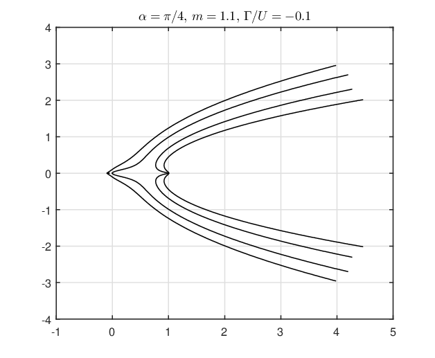
in the -parametric plane of some streamlines around the vortex are presented in Fig.3. Here, is given by (3.2), for the preimages of streamlines facing the infinite point of the wedge and of those facing the corner. The curves are symmetric with respect to the real axis. In Fig.3, the point is chosen to be , and , , respectively, while and . The vortex and the streamlines corresponding to their preimages in Fig. 3 for the same and are shown in Fig.4. Two cusps are seen at the points where the streamline branches and where the branches merge. The dashed line demonstrates the preimage of the straight path from to . Figures 5 a-b show the vortex domains and in cases b and c some streamlines around the vortex when and the angle (a), (b), and (c). It turns out that for angles the preimage of the straight path from to intersects the preimage of the contour (Fig. 5 d). It is also found that the streamlines close to the vortex boundary penetrate it. These results indicate that a vortex domain with the prescribed properties does not exist in wedges when Some other samples of vortices and streamlines nearby are given in Fig. 6 a-d. In Fig. 6 a and b, with and . In Fig. 6 c and d, with and . It is seen that when the conformal mapping free parameter grows the vorticity drifts out of the wedge corner. Fig. 6 a and b also show that when grows and approaches , the vortex sheet length grows as well, and the vortex domain moves away from the corner. The normalized tangential velocity on the horizontal side of the wedge is plotted for some and in Fig.7. It is seen that when the angle decreases, the speed is increasing. It is also observed that when decreases and the vortex becomes closer to the corner, the speed grows.
7 Conclusions
A two-dimensional flow of an inviscid incompressible fluid in a wedge with impenetrable walls about a Sadovskii vortex has been investigated by the method of conformal mappings. The shape of the vortex domain is unknown a priori, and no stagnation points on the wedge sides are admitted by the model. The map has been constructed by solving a symmetric Riemann-Hilbert problem on a finite and a semi-infinite segments lying on an elliptic Riemann surface. Owing to the asymptotics at infinity of the classical Weierstrass analogue of the Cauchy kernel for an elliptic surface and the right hand-side of the Riemann-Hilbert problem, the use of the Weierstrass kernel leads to divergent integrals. A new analogue of the Cauchy kernel on a hyperelliptic surface with properties required has been proposed, and a closed-form solution to the Riemann-Hilbert problem has been constructed. It is noted that the Weierstrass kernel would have worked if another map from the exterior of two finite segments on the flow domain had been applied. The initial authors’ efforts to numerically implement the procedure and recover such a map failed. On the contrary, the mapping from a finite and a semi-infinite two-sided segments onto the vortex boundary and the wedge walls, respectively, has been numerically successful. The conformal mapping recovered by solving the Riemann-Hilbert problem has a free geometric parameter and two problem parameters, the wedge angle and the ratio of the circulation and the speed on the vortex boundary. The vortex and the wedge boundaries have been determined by quadratures and numerically reconstructed. The vortex boundary formed by two branches of the same streamline in all numerical tests share the same feature of having two cusps. It has also been found that although for the wedge angle greater than , it is possible to reconstruct a vortex domain by solving the free boundary problem, the solution cannot be accepted as a physical one since streamlines close to the vortex domain penetrate he vortex interior. Thus the solution exists and has one free real parameter for and does not exist when .
Acknowledgments.
The authors thank the Isaac Newton Institute for Mathematical Sciences, Cambridge, for support and hospitality during the program Complex analysis: techniques, applications and computations, where a part of work on this paper was undertaken.
References
- [1] Y.A.Antipov, Method of Riemann surfaces for an inverse antiplane problem in an n-connected domain, Complex Var. Elliptic Equ., 65 (2020), pp. 455-480.
- [2] Y.A. Antipov and V.V. Silvestrov, Method of Riemann surfaces in the study of supercavitating flow around two hydrofoils in a channel, Phys. D, 235 (2007), pp. 72-81.
- [3] Y.A. Antipov and V.V. Silvestrov, Double cavity flow past a wedge, Proc. R. Soc. A., 464 (2008), pp. 3021-3038.
- [4] Y.A. Antipov and A.Y. Zemlyanova, Motion of a yawed supercavitating wedge beneath a free surface, SIAM J. Appl. Math., 70 (2009), pp. 923-948.
- [5] Y.A. Antipov and A.Y. Zemlyanova, Single- and double-spiral-vortex models for a supercavitating non-symmetric wedge in a jet, Proc. R. Soc. A., 465 (2009), pp. 3817-3837.
- [6] G. Birkhoff and E. H. Zarantonello, Jets, Wakes, and Cavities, Academic Press, New York, 1957.
- [7] G.R. Baker, P.G. Saffman, and J.S. Sheffield, Structure of a linear array of hollow vortices of finite cross-section, J. Fluid Mech., 74(3) (1976), pp. 469-476.
- [8] T.W. Christopher and S.G. Llewellyn Smith, Hollow vortex in a corner, J. Fluid Mech., 908 (2021), R2 1-12.
- [9] D. Crowdy, Solving Problems in Multiply Connected Domains, SIAM, Philadelphia, 2020.
- [10] J. D. Eshelby The determination of the elastic field of an ellipsoidal inclusion, and related problems, Proc. Roy. Soc. London A 241 (1957), pp. 376-396.
- [11] B. Gustafsson and A. Vasil’ev, Conformal and potential analysis in Hele-Shaw cells, Advances in Mathematical Fluid Mechanics. Birkhäuser Verlag, Basel, 2006
- [12] A.R. Low, Normal Elliptic Functions, University of Toronto Press, Toronto, 1950.
- [13] D.W. Moore, P.G. Saffman, S. Tanveer, The calculation of some Batchelor flows: the Sadovskii vortex and rotational corner flow, Phys. Fluids, 31 (1988), pp. 978-990.
- [14] H.C. Pocklington, The configuration of a pair of equal and opposite hollow straight vortices, of finite cross-section, moving steadily through fluid, Proc. Cambridge Philos. Soc., 8 (1895), 178-187.
- [15] V.S. Sadovskii, Vortex regions in a potential stream with a jump of Bernoulli’s constant at the boundary, J. Appl. Math. Mech. (PMM), 35 (1971), pp. 729-735.
- [16] P.G. Saffman, Vortex Dynamics, Cambridge University Press, Cambridge, 1992.
- [17] R. Vaglio-Laurin and M. H. Bloom, Chemical effects in external hypersonic flows. In Hypersonic Flow Research, Ed. F.R. Riddell, Academic Press, New York, 1962.
- [18] A.Y. Zemlyanova and Y.A. Antipov, Single-spiral-vortex model for a cavitating elastic curvilinear foil, SIAM J. Appl. Math., 72 (2012), pp. 280-298.
- [19] E. I. Zverovich, Boundary value problems in the theory of analytic functions in Hölder classes on Riemann surfaces, Russian Math. Surveys, 26 (1971), pp. 117–192,