arXiv:2010.07844v2 [cond-mat.mes-hall] 29 Oct 2020
Unitary Symmetry-Protected Non-Abelian Statistics of Majorana Modes
Jian-Song Hong
Thanks: These authors contribute equally to this work.
Affiliation: International Center for Quantum Materials and School of Physics, Peking University, Beijing 100871, China
Affiliation: Collaborative Innovation Center of Quantum Matter, Beijing 100871, China
Ting-Fung Jeffrey Poon
Thanks: These authors contribute equally to this work.
Affiliation: International Center for Quantum Materials and School of Physics, Peking University, Beijing 100871, China
Affiliation: Collaborative Innovation Center of Quantum Matter, Beijing 100871, China
Long Zhang
Affiliation: International Center for Quantum Materials and School of Physics, Peking University, Beijing 100871, China
Affiliation: Collaborative Innovation Center of Quantum Matter, Beijing 100871, China
Xiong-Jun Liu
Thanks: Correspondence addressed to: xiongjunliu@pku.edu.cn
Affiliation: International Center for Quantum Materials and School of Physics, Peking University, Beijing 100871, China
Affiliation: Collaborative Innovation Center of Quantum Matter, Beijing 100871, China
Affiliation: CAS Center for Excellence in Topological Quantum Computation, University of Chinese Academy of Sciences, Beijing 100190, China
Affiliation: Institute for Quantum Science and Engineering and Department of Physics, Southern University of Science and Technology, Shenzhen 518055, China
Abstract
Symmetry-protected topological superconductors (TSCs) can host multiple Majorana zero modes (MZMs) at their edges or vortex cores, while whether the Majorana braiding in such systems is non-Abelian in general remains an open question.
Here we uncover in theory the unitary symmetry-protected non-Abelian statisitcs of MZMs and propose the experimental realization. We show that braiding two vortices with each hosting unitary symmetry-protected MZMs generically reduces to independent sectors, with each sector braiding two different Majorana modes. This renders the unitary symmetry-protected non-Abelian statistics.
As a concrete example, we demonstrate the proposed non-Abelian statistics in a spin-triplet TSC which hosts two MZMs at each vortex and, interestingly, can be precisely mapped to a quantum anomalous Hall insulator. Thus the unitary symmetry-protected non-Abelian statistics can be verified in the latter insulating phase, with the application to realizing various topological quantum gates being studied. Finally, we propose a novel experimental scheme to realize the present study in an optical Raman lattice. Our work opens a new route for Majorana-based topological quantum computation.
In this work, we propose and establish a generic theory for non-Abelian statistics of MZMs protected by unitary symmetries. Unlike the TR symmetry, the unitary symmetry can generically protect non-Abelian statistics without suffering the dynamical symmetry breaking in the braiding process. We further demonstrate the proposed non-Abelian braiding for MZM pairs bound to vortex cores in a concrete model, which belongs to the family of spin-triplet TSCs spintri2003; spintri2006; spintri2008; spintri2010; spintri2010b; spintri2019. By mapping the TSC to a quantum anomalous Hall insulator (QAHI) with zero modes via particle-hole transformation, we realize the non-Abelian statistics and various quantum logic gates in the latter system. A novel scheme with experimental feasibility is proposed to for the realization based on the recently widely studied optical Raman lattices ORL2014; ORL2016; ORL2019; ORL2020, and the results are numerically verified.
Figure 1: Schematic diagrams for MZMs residing at vortices in a unitary symmetry-protected TSC. The gray circles with arrows denote vortices, the blue dots are MZMs, and the dashed lines represent the branch cuts of MZMs. (a) The braiding of multiple pairs of MZMs is reduced into mulitple individual sectors, each of which two MZMs independently. (b) The sketch of in the concrete model. The local MZMs and define a complex fermion . The non-local complex ferimons are defined by MZMs in different vortices.
Generic theory.–We start with the generic theory of the non-Abelian statistics for unitary symmetry-protected MZMs. Consider multiple MZMs localized at each edge or vortex core in a symmetry-protected TSC, and the couplings among them are excluded by unitary symmetries Kotetes2013; GilbertBernevig2014; XJLiu2014C4; Ryu2016review; Nagaosa2014. The braiding of two vortices exchanges the multiple pairs of MZMs as shown schematically in Fig. 1(a1).
Let the system described by the Hamiltonian have a unitary symmetry , i.e., and , with symmetry-protected MZMs at both the left and right hand side edges
or vortices. The symmetry protection implies that so that the coupling between two MZMs in the same vortex core (left for or right for ) is forbidden. The braiding is a unitary dynamical evolution with duration which can be described by time-ordering integral .
When the TSC satisfies unitary symmetry at all time for , the unitary evolution also satisfies the symmetry (see more details in Supplementary Material SM).
We define the effective braiding Hamiltonian via to characterize the braiding. Since the operator represents a unitary transformation of MZMs, the braiding
Hamiltonian is linear and takes the generic form due to unitary symmetry, which can be written in an off-diagonal matrix form in the bases . The mode is a proper linear transformation of SM. The unitary braiding operator can then be proven to be , where and are zero and identity matrices, respectively SM. It follows that , where the braiding operator
(1)
This result shows that braiding two vortices generically reduces to independent sectors, with each sector braiding two different Majorana modes due to the symmetry protection [Fig. 1(a2)]. In other words, during the braiding a MZM in one vortex can only effectively see one, rather than all MZMs in another vortex.
Figure 2: Numerical results of braiding two vortices with perturbations. (a) Evolution of MZM wave function in a full braiding. (b-c) Evolution with symmetry-preserving randomized chemical potential . (d) Evolution with symmetry-breaking s-wave pairing . The non-Abelian braiding is confirmed in (a-c) that after a full braiding at (similar for other MZMs), and breaks down in (d). The adiabatic condition is satisfied in that returns to unity after a single () and a full () braiding.
Here and .
Table 1: Examples for symmetry-preserving or symmetry-breaking terms in TSC and QAHI. The letter “P” (“B”) in the rightmost column means that the term preserves (breaks) the symmetry that protects the topology.
TSC
QAHI
Topology
✓
✓
✓
P
✗
✓
✗
P
✓
✗
✗
P
✓
✗
✗
P
✗
✓
✗
P
✓
✗
✗
P
✗
✓
✗
P
✗
✗
✓
B
TSC Model.–We apply the generic theory to a TSC, with the Cooper pairs in the state and . The Hamiltonian reads , where , and
(2)
Here and act on particle-hole and spin space, respectively. The bulk spectra are gapless if . This model possesses unitary symmetries , and . The MZMs in vortex are protected by and , but not by . The first seven rows in Table 1 show various perturbations that keep or . The last row shows a perturbation that breaks while not , but the MZMs in vortex are not protected. The bulk Chern number computed via is
for .
Two MZMs exist in each vortex for phase and obey non-Abelian statistics. The vortex can be introduced by taking , where depends on and are the polar coordinates. The vortex phase can be gauge-transformed into the operators via , which then obey the anti-periodic boundary condition. The two MZMs read
(3)
and , where is the normalization factor, and . The two MZMs are protected by the unitary symmetry or , which also protects the non-Abelian statistics. The non-Abelian braiding and symmetry protection are confirmed by numerical simulation shown in Fig. 2 through a lattice Hamiltonian (see Supplemental Material SM). As predicted, each MZM (e.g. ) in braiding accumulates a phase after a full braiding [Fig. 2(a)]. This braiding result is robust against randomized chemical potential with , which preserves the symmetries [Fig. 2(b-c)]. Similar results are expected for other disorders without breaking the or symmetry. In comparison, a symmetry-breaking -wave superconducting order vitiates the braiding.
There are different ways to introduce the complex fermion modes from the MZMs, as illustrated in Fig. 1 (b). One is to define the complex fermion modes in non-local bases , and another is from local MZMs in each vortex as . (i) In the -representation, the MZMs are classified into two sectors denoted by and , and
the braiding operators can be generally decomposed into a direct product of the matrices of each sector.
For example, for four vortices, the Fock space is spanned by , which denotes states with particle number for .
In the subspace {,,,},
the braiding matrix of is
(4)
which connects states with the same fermion parity in each sector. (ii) In the -representation, there is a “particle-number conservation” due to the relation , with . We initialize the non-local fermion states as follows. Consider vortices (or anti-vortices) in TSC and couple them via . Here the phases of and have been absorbed into , and the eigenstates are . The braiding evolves the state of the system in the particle-number conserved subspaces. For example, in
the single-particle subspace for four vortices {,,,},
where denotes states with particle number for ,
the matrix of operator is
(5)
Under , each basis vector evolves into the superposition
of all the single-particle states. Note that is generally a linear
combination of and , and the particle-number conservation for and the parity conservation for are not contradictive.
Simulation of the non-Abelian statistics by QAHI.– We show now a highly nontrivial result that the unitary symmetry-protected non-Abelian statistics of MZM pairs can be mapped to and simulated by vortex modes in a QAHI. After the transformation and the replacements and , the Hamiltonian (2) describes a QAHI with vortices:
(6)
where and . The operator that annihilates the zero mode is just after particle-hole transformation. Noted that our realization of zero modes in a QAHI is different from the traditional proposal by digging a hole with a flux threading through ShenBook. In above Hamiltonian (6), we only introduce a phase vortex for . Similar to the case of the TSC model, the topology is protected by and . Table 1 shows examples of perturbation that keep or break the symmetry. To illustrate the nontrivial braiding statistics, we consider four vortices (or anti-vortices) in a QAHI so that there are four zero modes , , and [see Fig. 3(a)]. We initialized the system in the state and perform a numerical simulation in position space, as shown in Fig. 3(b-c). In the braiding, and travels away from their initial locations such that only overlaps with or [Fig. 3(b)]. After braiding once, the state evolves into a linear combination of the four states as expected in Eq. (5), and after a full braiding, the state evolves into . Further, we demonstrate the robustness of non-Abelian braiding against perturbations which keep the symmetries. As shown in Fig. 3(c), the full braiding transforms the negative energy state into the positive energy one ; the disorder in only induces fluctuations but cannot affect the braiding result.
[t]
Figure 3: Numerical simulation of a full braiding between and . (a) Orange ball denotes the lattice
sites, and Vortices (anti-vortices) are denoted by blue (red) circles. (b) The evolution of wave function . The system evolves into a superposition of the four single particle states as braiding
and once. After a full braiding,
evolves into . (c) The energy of as a function of time. The absolute
value of is denoted by . The
dashed lines show the energy evolution with certain randomization
in the term. After a full braiding, all the
three curves arrive at the positive energy , demonstrating
the robustness of non-Abelian statistics.
Here we set and .
We can realize various topological quantum gates by braiding the vortices. Due to the particle-number conservation, the realization of quantum logic gates in a QAHI is restricted in the -representation. For different subspaces, there are different methods to realize quantum logic gates. For example, in the two-particle subspace and defining , , , , we have
(7)
More vortices can be added to provide ancilla qubits. When considering six
vortices, one can define , , , as the four practical
qubits (the remaining two single-particle states serve as ancilla ones). We then have
(8)
Compared with previous realization of quantum logic gates utilizing
Majorana qubits Pachos2017, the current proposal provides simpler methods to realize CNOT-gate.
Figure 4: (a) Sketch of the experimental realization scheme. The atoms reside at a primary checkerboard lattice (black lines) with a staggered onsite Zeeman potential .
The Raman potential induces the spin-flip nearest neighbor hopping. A shaking lattice is applied to drive the spin-conserved hopping by compensating neighboring onsite energy difference. (b) The phase of Raman potential with . (c) The phase of the spin-flip hopping in the -direction produced by the Raman potential with . (d) The energy spectrum of the system with a vortex () and an anti-vortex (). See details in ref. SM.
Experimental realization.–Finally we propose a feasible experimental setup to simulate a QAHI with vortices via an optical Raman lattice ORL2014; ORL2016; ORL2019; ORL2020. The realization scheme is depicted in Fig. 4(a), and the details can found in the Supplemental Material SM. Besides the primary square lattice, there are three main ingredients in our proposal:
(i) Raman potential with an orbital angular momentum , which induces spin-flip hopping -term and the phase vortex. The orbital angular momentum can be imprinted by applying an Laguerre-Gaussian (LG) beam LG1; LG2.
(ii) Staggered on-site Zeeman term , which provides an on-site energy difference between the two spin states so that on-site spin flipping is suppressed.
(iii) Shaking lattice , which is applied to induce spin-conserved nearest-neighbor hopping.
We confirm by exact numerical calculations that such a realization indeed simulates a QAHI with vortices described by the Hamiltonian (6). We first calculate the phase of Raman potential in the case .
As in Fig. 4(b), the winding of the phase is along a path encircling the center of LG beam, while for any other paths encircling one center of lattice barrier, the winding is . The additional winding causes the spin-flip hopping to have a phase vortex at the center of the LG beam, as numerically demonstrated in Fig. 4(c).
We then calculate the energy spectrum of the system with a vortex () and an anti-vortex () SM.
The result is shown in Fig. 4(d). One can find two nearly degenerate states at the center of the gap, which confirms the existence of zero modes in vortices. The braiding of zero modes can then be realized by slowly moving the LG beam. Details of the realization are seen in ref. SM.
Conclusion.–We have uncovered that Majorana modes protected by unitary symmetries generically obey symmetry protected non-Abelian statistics, and proposed the experimental realization. Specifically, the MZM pairs in vortex cores of a unitary symmetry-protected spin-triplet TSC exemplify the non-Abelian statistics with analytical and numerical results. In comparison with TSCs without symmetry-protection, the Majorana qubit states with unitary symmetry-protection can be defined in the local and non-local bases, which facilitate the realization of various topological quantum gates. We further mapped the spin-triplet TSC to QAHI, with which we proposed a practical experimental scheme in optical Raman lattice to verify the present study. This work enriches the braiding statistics and may open up diverse routes toward realizing topological quantum computers.
References
(1) A. Y. Kitaev, Physics-Uspekhi 44, 131 (2001).
(2) N. Read and D. Green, Phys. Rev. B 61, 10267 (2000).
(3) C. Nayak, S. H. Simon, A. Stern, M. Freedman, and S. Das Sarma, Rev. Mod. Phys. 80, 1083 (2008).
(4) C. Nayak and F. Wilczek, Nucl. Phys. B 3, 529 (1996).
(5) D. A. Ivanov, Phys. Rev. Lett. 86, 268 (2001).
(6) S. Das Sarma, M. Freedman, and C. Nayak, Phys. Rev. Lett. 94, 166802 (2005).
(7) J. Alicea, Y. Oreg, G. Refael, F. Von Oppen, and M. P. Fisher, Nat. Phys. 7, 412 (2011).
(8) A. Kitaev, Annals of Physics 303, 2 (2003).
(9) D. Aasen, M. Hell, R. V. Mishmash, A. Higginbotham, J. Danon, M. Leijnse, T. S. Jespersen, J. A. Folk, C. M. Marcus, K. Flensberg, and J. Alicea, Phys. Rev. X 6, 031016 (2016).
(10) V. Lahtinen and J. K. Pachos, SciPost Phys. 3, 021 (2017).
(11) V. Mourik, K. Zuo, S. M. Frolov, S. Plissard, E. P. Bakkers, and L. P. Kouwenhoven, Science 336, 1003 (2012).
(12) M. Deng, C. Yu, G. Huang, M. Larsson, P. Caroff, and H. Xu, Nano Letters 12, 6414 (2012).
(13) L. P. Rokhinson, X. Liu, and J. K. Furdyna, Nat. Phys. 8, 795 (2012).
(14) A. Das, Y. Ronen, Y. Most, Y. Oreg, M. Heiblum, and H. Shtrikman, Nat. Phys. 8, 887 (2012).
(15) M.-X. Wang, C. Liu, J.-P. Xu, F. Yang, L. Miao, M.-Y. Yao, C. L. Gao, C. Shen, X. Ma, X. Chen, Z.-A. Xu, Y. Liu, S.-C. Zhang, D. Qian, J.-F. Jia, and Q.-K. Xue, Science 336, 52 (2012).
(16) H. O. H. Churchill, V. Fatemi, K. Grove-Rasmussen, M. T. Deng, P. Caroff, H. Q. Xu, and C. M. Marcus, Phys. Rev. B 87, 241401 (2013).
(17) J.-P. Xu, C. Liu, M.-X. Wang, J. Ge, Z.-L. Liu, X. Yang, Y. Chen, Y. Liu, Z.-A. Xu, C.-L. Gao, D. Qian, F.-C. Zhang, and J.-F. Jia, Phys. Rev. Lett. 112, 217001 (2014).
(18) S. Nadj-Perge, I. K. Drozdov, J. Li, H. Chen, S. Jeon, J. Seo, A. H. MacDonald, B. A. Bernevig, and A. Yazdani, Science 346, 602 (2014).
(19) W. Chang, S. Albrecht, T. Jespersen, F. Kuemmeth, P. Krogstrup, J. Nygård, and C. M. Marcus, Nature Nanotechnology 10, 232 (2015).
(20) S. M. Albrecht, A. P. Higginbotham, M. Madsen, F. Kuemmeth, T. S. Jespersen, J. Nygård, P. Krogstrup, and C. Marcus, Nature 531, 206 (2016).
(21) J. Wiedenmann, E. Bocquillon, R. S. Deacon, S. Hartinger, O. Herrmann, T. M. Klapwijk, L. Maier, C. Ames, C. Brüne, C. Gould, A. Oiwa, K. Ishibashi, S. Tarucha, H. Buhmann, and L. W. Molenkamp, Nature Communications 7, 1 (2016).
(22) E. Bocquillon, R. S. Deacon, J. Wiedenmann, P. Leubner, T. M. Klapwijk, C. Brüne, K. Ishibashi, H. Buhmann, and L. W. Molenkamp, Nature Nanotechnology 12, 137 (2017).
(23) K. Zhang, J. Zeng, Y. Ren, and Z. Qiao, Phys. Rev. B 96, 085117 (2017).
(24) P. Zhang, K. Yaji, T. Hashimoto, Y. Ota, T. Kondo, K. Okazaki, Z. Wang, J. Wen, G. D. Gu, H. Ding, and S. Shin, Science 360, 182 (2018).
(25) D. Wang, L. Kong, P. Fan, H. Chen, S. Zhu, W. Liu, L. Cao, Y. Sun, S. Du, J. Schneeloch, R. Zhong, G. Gu, L. Fu, H. Ding, and H.-J. Gao, Science 362, 333 (2018).
(26) A. Fornieri, A. M. Whiticar, F. Setiawan, E. Portolés, A. C. Drachmann, A. Keselman, S. Gronin, C. Thomas, T. Wang, R. Kallaher, G. C. Gardner, E. Berg, M. J. Manfra, A. Stern, C. M. Marcus, and F. Nichele, Nature 569, 89 (2019).
(27) H. Ren, F. Pientka, S. Hart, A. T. Pierce, M. Kosowsky, L. Lunczer, R. Schlereth, B. Scharf, E. M. Hankiewicz, L. W. Molenkamp, B. I. Halperin, and A. Yacoby, Nature 569, 93 (2019).
(28) B. Jåck, Y. Xie, J. Li, S. Jeon, B. A. Bernevig, and A. Yazdani, Science 364, 1255 (2019).
(29) X.-L. Qi, T. L. Hughes, S. Raghu, and S.-C. Zhang, Phys. Rev. Lett. 102, 187001 (2009).
(30) J. C. Y. Teo and C. L. Kane, Phys. Rev. B 82, 115120 (2010).
(31) A. P. Schnyder, P. M. R. Brydon, D. Manske, and C. Timm, Phys. Rev. B 82, 184508 (2010).
(32) C. W. J. Beenakker, J. P. Dahlhaus, M. Wimmer, and A. R. Akhmerov, Phys. Rev. B 83, 085413 (2011).
(33) C. L. M. Wong and K. T. Law, Phys. Rev. B 86, 184516 (2012).
(34) S. Nakosai, Y. Tanaka, and N. Nagaosa, Phys. Rev. Lett. 108, 147003 (2012).
(35) F. Zhang, C. L. Kane, and E. J. Mele, Phys. Rev. Lett. 111, 056402 (2013).
(36) A. Keselman, L. Fu, A. Stern, and E. Berg, Phys. Rev. Lett. 111, 116402 (2013).
(37) A. Haim and Y. Oreg, Physics Reports 825, 1 (2019).
(38) X.-J. Liu, C. L. M. Wong, and K. T. Law, Phys. Rev. X 4, 021018 (2014).
(39) P. Gao, Y.-P. He, and X.-J. Liu, Phys. Rev. B 94, 224509 (2016).
(40) M. McGinley and N. R. Cooper, Phys. Rev. Lett. 121, 090401 (2018).
(41) K. Wölms, A. Stern, and K. Flensberg, Phys. Rev. Lett. 113, 246401 (2014).
(42) K. Wölms, A. Stern, and K. Flensberg, Phys. Rev. B 93, 045417 (2016).
(43) C. Knapp, A. Chew, and J. Alicea, arXiv: 2006.10772.
(44) A. P. Mackenzie and Y. Maeno, Rev. Mod. Phys. 75, 657 (2003).
(45) S. Das Sarma, C. Nayak, and S. Tewari, Phys. Rev. B 73, 220502 (2006).
(46) X. Dai, Z, Fang, Y. Zhou, and F. -C. Zhang, Phys. Rev. Lett. 101, 057008 (2008).
(47) J. D. Strand, D. J. Bahr, D. J. Van Harlingen, J. P. Davis, W. J. Gannon, and W. P. Halperin, Science 328, 1368 (2010).
(48) L. Fu and E. Berg, Phys. Rev. Lett. 105, 097001 (2010).
(49) S. Ran, C. Eckberg, Q. -P. Ding, Y. Furukawa, T. Metz, S. R. Saha, I.-L. Liu, M. Zic, H. Kim, J. Paglione, and N. P. Butch, Science 365, 684 (2019).
(50) X. -J. Liu, K. -T. Law, and T. -K. Ng, Phys. Rev. Lett. 112, 086401 (2014).
(51) Z. Wu, L. Zhang, W. Sun, X. -T. Xu, B. -Z. Wang, S. -C. Ji, Y. Deng, S. Chen, X. -J. Liu, and J. -W. Pan, Science 354, 83 (2016).
(62) L. Allen, M. W. Beijersbergen, R. J. C. Spreeuw, and J. P. Woerdman, Phys. Rev. A 45, 8185 (1992).
(63) G. Juzeliūnas and P. Öhberg, Phys. Rev. Lett. 93, 033602 (2004).
Supplemental Material
In this Supplemental Material, we provide details for the generic theory of unitary symmetry-protected non-Abelian statistics, the model Hamiltonian for TSC, the braiding matrices in different representations and the experimental realization.
I Unitary symmetry protection
In this section, we show in general that in a unitary symmetry-protected TSC, the braiding of two vortices with each hosting multiple Majorana modes can be reduced into multiple independent sectors, each of which braids independently, leading to the symmetry-protected non-Abelian statistics. The braiding process is described by the evolution operator
(S1)
where is the time-ordering operator. If the system keeps a unitary symmetry throughout the braiding process, i.e. at any time for , where is the total braiding time and is the unitary symmetry that protects the topology, the effective Hamiltonian also satisfies the symmetry since
(S2)
so that . Now we consider the case with each vortex binding Majorana modes (), between each pair of the Majorana modes, e.g. and there is a unitary sub-symmetry providing the protection. Note that since the braiding process is a unitary transformation which exchange the positions of two vortices, the effective Hamiltonian must be a
linear one in terms of Majorana operators. The effective Hamiltonian takes
the generic form since the local coupling is excluded by the protection of unitary symmetries. So in the Majorana bases, the effective Hamiltonian can be rewritten as
(S3)
where is a real matrix. The braiding operator , in which
(S4)
The braiding process exchanges the left and right hand vortices, so the left and right hand side MZMs must exchange positions, and accordingly the diagonal elements in must vanish by definition. Then only
the off-diagonal blocks survive, giving
(S5)
Since is unitary, one can verify that is also unitary. Therefore by noting that , which means each MZM accumulates a phase after full braiding. The phase after a single braiding can be fixed by
so that
(S6)
This implies that under unitary symmetry protection, the MZMs can always be effectively reduced into several individual sectors, which are characterized by the braiding operator given by Eq. (1) of the main text. Note that in general can be a complicated superposition of s, depending on the details of the braiding process and the static Hamiltonian. However, during the braiding a MZM in one vortex can only effectively see one, rather than all MZMs in another vortex. This essentially renders the symmetry-protected non-Abelian statistics.
II Model Hamiltonian
The tight-binding Hamiltonian for our model TSC is
(S7)
and the model is protected by unitary symmetries , whose second-quantized forms are . It’s convenient to rewrite the Hamiltonian in -space, , where and the phase of is absorbed into the definition of . In the continuum limit, the single-particle BdG Hamiltonian is transformed into (2) with and . The vortex in this system traps two MZMs in topological phase, and in the limit , they take the form
(S8)
(S9)
The MZMs will be transformed by the symmeties as , and , , which means the pair of MZMs are symmetry-protected.
III Braiding matrices
The braiding operator
is particle-number conserved in the -representation thus the braiding matrices are block-diagonal in particle-number conserved
subspaces. For four vortices, the state of system can be generally written as
,
where denotes the particle number of .
In the one-particle subspace ,
or three-particle subspace {,
, ,
}, the braiding operators are
(S10)
The operator only affects while combines all four states. In the two-particle subspace {,
, ,
, ,
}, the braiding operators are
(S11)
The braiding operators act trivially on the vaccum state and four-particle
state .
In the -representation, braiding operator
is parity-conserved in sectors and , and the braiding matrices
are direct product of matrices in each sector. The particle-number
conservation of and the parity conservation of are not
contradictory since is generally the linear combination of
and , for example, ,
and therefore the vaccum states and
are different. For four vortices, the state of system can be generally written as
, where
denotes the particle-number of . The whole Fock space can be divided into even and odd parity parts of sectors
(S12)
Braiding matrices in a single sector can be written in even and odd parity subspaces S 1
(S13)
Figure S1: Experimental realization in an optical Raman lattice. (a) Experimental setup.
With the bias magnetic field applied in the direction, the light components (red)
form a spin-independent checkerboard lattice, and generate periodic Raman coupling potentials together with the circularly polarized beam incident along the -axis. The light is set to be
a Laguerre-Gaussian (LG) beam carrying optical vortices, which imprints a spatially-dependent phase on spin-flipped hoppings.
Two beam components of (blue) with mutually perpendicular polarization is used to produce a spin-dependent lattice in the direction, which provides a staggered Zeeman energy splitting.
Two beams are applied along the and directions respectively to form a 2D shaking lattice by sinusoidally modulating the phases of retro-reflected components via electro-optic modulators (EOMs). (b) The contour plot of the lattice potentials and (upper panel). Their combination produces a staggered on-site energy difference for the two spin states (lower panel).
Here .
IV Experimental realization
We propose an experimental setup based on the optical Raman lattice scheme which was used to realize Weyl semimetal in 3D S 2; S 3, as sketched in Fig. S1.
We aim to realize the Hamiltonian
(S14)
where is the primary checkerboard lattice, denotes the Raman coupling potential with a spatially-dependent phase,
is a spin-dependent lattice, which provides a staggered Zeeman splitting at each lattice site and thus suppresses the on-site spin flipping,
and is a two-dimensional (2D) shaking lattice, which is applied to induce and control the spin-conserved nearest-neighbor hopping.
IV.1 Primary checkerboard lattice and Raman coupling potential
As shown in Fig. S1(a), the beams of frequency with -polarization and of frequency () with -polarization together form a 2D standing waves in the - plane via mirror reflection, where
(S15)
Note that the relative phase between the - and -polarized components acquires a phase after passing through the quarter-wave plate () twice.
When , the standing wave leads to a checkerboard lattice S 2, which takes the form
(S16)
where , , , and .
We further apply a circularly polarized Laguerre-Gaussian (LG) beam of frequency in the direction, which carries an orbital angular momentum .
The light field can be written as
(S17)
where is the azimuthal angle.
If with being the Zeeman splitting of the two spins,
the Raman potential can be generated through the double--type coupling configuration via the standing wave and the running wave , which reads
(S18)
with .
IV.2 Spin-dependent lattice
Two lights with mutually perpendicular polarization are applied in the - plane to generate a spin-dependent lattice in the direction,
which are incident from the positive and negative -axis, respectively, with the angles to the z-axis being both [see Fig. S1(a)].
The light field reads
(S19)
The spin-dependent lattice is the vector light shift S 4; S 5, thus taking the form
(S20)
with . As shown in Fig. S1(b), the combination of the primary lattice (S16) plus the spin-dependent lattice (S20) indeed provides a staggered on-site Zeeman term.
Note that for a realistic setup, one need to choose proper hyperfine states to construct the spin- system such as the -induced spin-independent part can be neglected.
For example, one can choose and for 40K atoms S 6.
IV.3 Shaking lattice
The shaking lattice is formed by two beams of wavelength applied in the and directions, respectively,
with the phases of their retro-reflected components being sinusoidally modulated S 7; S 8.
The light fields are
(S21)
Hence, the shaking lattice potential reads
(S22)
where and with being the shaking amplitude and .
IV.4 Tight-binding model
In this subsection, we consider the tight-binding limit of the total Hamiltonian (S14).
We denote as the Wannier function of spin for -bands of .
Without loss of generality, we suppose .
The spin-flipped hopping is
(S23)
where denotes the lattice constant.
Due to the identity
(S24)
where are the Bessel functions,
the shaking lattice potential can be written as , where
(S25)
The shaking-induced spin-conserved hopping can be written as
(S26)
With these ingredients the tight-binding model of QAHI is realized and given by Eq. (S7) after particle hole transformation as introduced in main text.
IV.5 Numerical Results
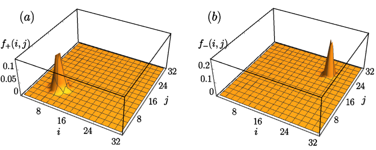
In the numerical simulation, we apply two LG beams that carry opposite angular momentum to eliminate the winding of Raman potential at the boundary. We confirmed that there are two almost degenerate eigenstates localized at the centers of the LG beams which energies are at the center of the gap opened by spin-orbit coupling. The remaining non-degeneracy is the result of two reasons - (i) There are residue effective or that are not canceled by the onsite staggered term, and (ii) the strength of is spin and site dependent since the size of the barrier that are overcome by the Raman coupling has staggered pattern. The split of energy is about of the size of the gap with , and . Let be the wavefunctions of two zero modes and , where the integration is done in the region of the site , be the site-wise probability of the states. Fig. S2(a-b) show and the zero modes are localized at the centers of the vortex or anti-vortex.
Figure S2: of two zero-modes which are localized at the vortex or anti-vortex respectively. The vortex is located at the barrier between and , and the anti-vortex is located at the barrier between and .
References
S (1) J. Alicea, Rep. Prog. Phys. 75, 076501 (2012).
S (2) Y.-H. Lu, B.-Z. Wang, and X.-J. Liu, arXiv:1911.07169.
S (3) Z.-Y. Wang, X.-C. Cheng, B.-Z. Wang, J.-Y. Zhang, Y.-H. Lu, C.-R. Yi, S. Niu, Y. Deng, X.-J. Liu, S. Chen, and J.-W. Pan, arXiv:2004.02413.
S (4) I. H. Deutsch and P. S. Jessen, Phys. Rev. A 57, 1972 (1998).
S (5) O. Mandel, M. Greiner, A. Widera, T. Rom, T. W. Hänsch, and I. Bloch, Phys. Rev. Lett. 91, 010407 (2003).
S (6) Y. Wang, L. Zhang, S. Niu, D. Yu, and X.-J. Liu, Phys. Rev. Lett. 125, 073204 (2020).
S (7) N. Gemelke, E. Sarajlic, Y. Bidel, S. Hong, and S. Chu, Phys. Rev. Lett. 95, 170404 (2005).
S (8) C. V. Parker, L.-C. Ha, and C. Chin, Nat. Phys. 9, 769 (2013).