LiteDepthwiseNet: An Extreme Lightweight Network for Hyperspectral Image Classification
Abstract
Deep learning methods have shown considerable potential for hyperspectral image (HSI) classification, which can achieve high accuracy compared with traditional methods. However, they often need a large number of training samples and have a lot of parameters and high computational overhead. To solve these problems, this paper proposes a new network architecture, LiteDepthwiseNet, for HSI classification. Based on 3D depthwise convolution, LiteDepthwiseNet can decompose standard convolution into depthwise convolution and pointwise convolution, which can achieve high classification performance with minimal parameters. Moreover, we remove the ReLU layer and Batch Normalization layer in the original 3D depthwise convolution, which significantly improves the overfitting phenomenon of the model on small sized datasets. In addition, focal loss is used as the loss function to improve the model’s attention on difficult samples and unbalanced data, and its training performance is significantly better than that of cross-entropy loss or balanced cross-entropy loss. Experiment results on three benchmark hyperspectral datasets show that LiteDepthwiseNet achieves state-of-the-art performance with a very small number of parameters and low computational cost.
Index Terms:
depthwise convolution, focal loss, lightweight network, hyperspectral image classification.I Introduction
In recent years, as a kind of optical remote sensing image with high spectral resolution, hyperspectral images (HSIs) have attracted much attention because of their unique properties and the massive information they contain [1]. HSIs have been widely used in mineral exploration [2], soil salinity estimation [3], and anomaly detection [4]. At present, HSI classification is one of the most active research areas in the remote sensing field. Its goal is to classify each marked pixel in the image correctly, where a pixel can be regarded as a high-dimensional vector with each entry corresponding to the spectral reflectance in a specific wavelength [5].
Early work on HSI classification mainly focused on exploring spectral feature information and ignoring spatial information [6, 7, 8, 9, 10], which often leads to poor generalization performance. After this, some studies began to incorporate spatial contextual information into pixel-level classifiers. Representative work includes extended morphological profiles (EMP) [11, 12], edge-preserving filtering [13] and sparse representation models [14, 15, 16, 17, 18], etc. Due to the spatial homogeneous characteristics of HSI, spectral-spatial HSI classification methods usually show better results than spectral-based methods. Notwithstanding, most of spectral-spatial methods depend on hand-crafted or shallow features, which are usually designed for specific tasks and rely on expert knowledge. This largely limits the flexibility and applicability of these methods in difficult situations.
Recently, deep learning (DL) methods have been applied in HSI classification successfully. The earlier DL-based HSI classification methods based on fully connected neural networks, such as stacked autoencoders (SAEs) [19] and recursive autoencoders (RAEs) [20], can only handle one-dimensional vectors. Thus, the spatial structure information of an HSI is destroyed. The emergence of convolutional neural networks (CNNs) overcomes this defect. Several 2D CNN based architectures were proposed, including R-VCANet [21] and bayesian 2D CNN [22], etc. However, a HSI has too many channels, which often causes 2D convolution kernels to be too deep, and there is also a significant increase in the number of parameters. Therefore, 3D CNN based HSI classification methods were proposed. Lee et al. [23] described a contextual deep CNN by applying multiple 3D local convolutional filters with different sizes to jointly exploit the spatial and spectral features of a HSI. Chen et al. [24] established a 3D CNN-based feature extraction model with regularization to extract the effective spectral-spatial features of HSIs. Hamida et al. [25] proposed a new 3D deep learning method that can simultaneously process spectral and spatial information while incurring lower computation cost (i.e. floating point operations, FLOPs). Although 3D CNN can reduce the number of parameters, it still incurs more calculational consumption because it needs to traverse in depth and lacks a global view of spectral information. HybridSN, a recent work proposed by Roy et al. in [26], combined 2D CNN and 3D CNN, where 3D CNN was used to mine spatial and spectral information and 2D CNN integrated the information to output the prediction result. It can effectively improve classification accuracy and has a global view to integrate spectral features. However, without an end-to-end architecture, PCA was still used to compress the redundant spectral information, which adds computational cost.
Although the aforementioned DL models have shown excellent HSI classification performance, they usually need a large number of training samples and network parameters, and also have higher computational cost. For HSI classification, the available labeled pixels are usually very limited due to the difficulty in collecting and cost in labeling. Moreover, the distribution of categories in these labeled data is imbalanced. Constructing robust DL models with high performance and low computational cost based on imbalanced and small sample-sized data is a huge challenge in this field. Recently, a lightweight neural network, LiteDenseNet [27], has been proposed for HSI classification. Different from traditional 3D CNN architectures, LiteDenseNet has a 3D two-way dense structure and uses group convolution, which greatly reduces the number of parameters and computational cost. However, the group convolution cuts off the connection of different channels and may lead to a loss of accuracy. To solve this problem and further reduce the parameters, we propose an extremely lightweight network, LiteDepthwiseNet, for HSI classification tasks. Its main advantages are summarized as follows.
- 1.
A 3D depthwise convolution is used to replace the group convolution. The pointwise convolution in the 3D depthwise convolution can connect all hyperspectral channels, and the corresponding network architecture has a full-channel receptive field and is more suitable for HSI classification task. Based on this new network architecture, LiteDepthwiseNet only involves a very small number of parameters and FLOPs.
- 2.
Focal loss (FL) is introduced to replace mainstream cross entropy loss (CEL) as the loss function. It increases the attention on small sample categories and difficult-to-classify samples, which helps to improve the ultimate performance of the model.
- 3.
The middle activation layer and normalization layer in the original 3D depthwise convolution network are stripped, which can enhance the linearity of the model, so as to reduce the overfitting phenomenon when there are few training samples for HSIs.
The rest of this paper is arranged as follows. In Section II, we briefly introduce the related work. The structure of the proposed LiteDepthwiseNet is detailed in Section III. The comparison experiment results of seven algorithms on three well-known HSI datasets are reported in Section IV. Section V summarizes this paper.
II Related work
This section describes some related concepts and gives a brief introduction to LiteDenseNet, which inspires the main design of the proposed network architecture in this paper.
II-A 2D depthwise separable convolution
Different from standard convolution, the depthwise separable convolution proposed in [28] includes a depthwise convolution, i.e. a spatial convolution performed independently over each channel of an input, followed by a pointwise convolution, i.e. a convolution, projecting the channels output by the depthwise convolution onto a new channel space. Figs. 1 and Figs. 2 show a simple schematic of a standard convolution and a depthwise separable convolution, respectively.
By splitting the standard convolution into two processes of depthwise convolution and pointwise convolution, the computational cost and the number of parameters in the 2D convolution can be significantly reduced under certain conditions.


II-B Cross entropy loss
The CEL function is a loss function often used in classification problems. It is an important concept in information theory, where it is mainly used to measure the difference between two probability distributions.
The standard CEL for classification problems is,
| (1) |
where represents the predicted probability of a sample in the category, and , an indicate variable equal to 0 or 1, represents whether the sample is correctly classified. It can be observed that when is , the closer the is to , the smaller the loss and if is , the closer the is to 0, the smaller the loss, which is in line with the direction of optimization.
To simplify the expression, we introduce a piecewise function as:
| (2) |
and then the standard CEL can be reformulated as:
| (3) |
In order to handle data with imbalanced categories, a coefficient is added to the standard cross-entropy loss function to balance the weights of samples of different categories, which results in the following balanced CEL (BCEL):
| (4) |
II-C LiteDenseNet
In 2020, Li et al. [27] proposed a lightweight network LiteDenseNet. To obtain receptive fields in different scales, the network uses a 3D two-way dense layer which was proposed in PeleeNet [29] and DBDA [30]. Its schematic diagram is shown in Fig. 3.

This 3D two-way dense layer comprises a top layer and a bottom layer. After performing a convolution transformation on the input data, the top layer uses a two stacked convolution to capture global features and obtains an output with size , and the bottom layer uses a convolution kernel with size to capture local features and obtains an output with size . The outputs of the two-way dense layer are used to perform the concatenate operation to generate a 3D-cube with size .
However, the 3D convolutional block in the original 3D two-way dense layer is a computationally intensive model. In order to reduce the number of parameters and computational cost, LiteDenseNet uses group convolution instead of normal convolution. The group convolution given in [27] is shown in Fig. 4.

Given an input data with size and channels, the normal convolution layer tends to have the same channel size as the inputs, whereas the group convolution divides the original convolution kernels and the input into 3 groups by channel dimension. As a result, the input is divided into three groups with the size of and channels . Three groups are fed into a normal convolution with the channels separately. So the channel size is reduced from to . In this way, group convolution significantly reduces the number of parameters and computational cost while maintaining the size of the input and the output.
III The proposed LiteDepthwiseNet
In this section, we describe the proposed LiteDepthwiseNet in detail.
III-A Modified 3D Depthwise Convonlution
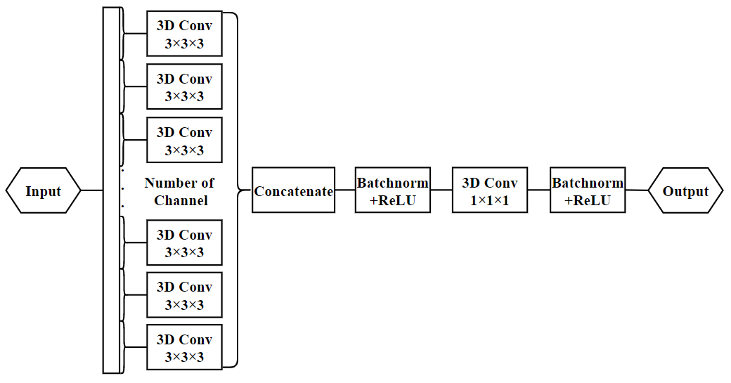
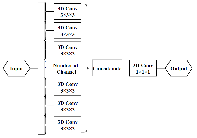
LiteDenseNet reduces the parameters and computational cost using group convolution to replace standard convolution. However, group convolution permanently cuts off some connections between channels, which results in reducing the classification performance to some extent. Moreover, for HSI classification, there is still room to reduce the parameters and computational cost. So, we consider replacing group convolution with depthwise separable convolution, in which pointwise convolution can connect all the channels. At the same time, for HSIs, there are too many channels, so 2D depthwise separable convolution will still have too many parameters. A good choice is to use 3D depthwise convolution originally proposed in [31] for RGB images. At this point, a new problem appears. The limited number of training samples for HSIs always causes overfitting for the model which has a too strong nonlinear ability. So, we propose a modified 3D depthwise convolution for HSI classification. The major adjustment is that the middle activation layer and normalization layer of the original 3D depthwise convolution network are stripped, which enhances the linearity of the model and reduces the overfitting phenomenon. Moreover, the number of parameters and the computational consumption are greatly reduced. Structural comparison diagrams of group convolution, 3D depthwise convolution and modified 3D depthwise convolution are shown in Figs. 5, 6, and 7, respectively.

III-B Focal Loss
Since most HSIs have imbalanced data categories [5], using the standard CEL function for training will lead to low classification accuracy for the small sample categories. The BCEL function is commonly used to deal with this situation. However, the BCEL function is also likely to focus on the easy-to-classify samples. In order to improve the classification performance, the model should focus on both small-category samples and difficult-to-classify samples. For this purpose, a focal loss is proposed in [32] and expressed as
| (5) |
where
From formula (5), it is easy to know the following three points. Firstly, similar to the BCEL, parameter is introduced to reflect the imbalanced problem of different categories of samples, which helps to improve the accuracy of the final model. Secondly, the modulating factor is added to adjust the weights of easy-to-classify samples and difficult-to-classify samples. When a sample is misclassified and is small, then is close to 1, and the loss is not affected. However, if , which indicates that the classification prediction of the sample is better, is 0, and the loss is down-weighted. Lastly, the focusing parameter smoothly adjusts the down-weighted rate of easy-to-classify samples. When , the FL is equivalent to the BCEL and with the increase of , the effect of the modulating factor also increases. Of these, can be set by category frequency, or it can be obtained as a hyperparameter for cross-validation.
III-C The Framework of the LiteDepthwiseNet
The overall framework of the proposed LiteDepthwiseNet and the specific parameters in an example are shown in Fig. 8 and Table I, respectively.

Specifically, in our network framework, batch normalization (BN) and ReLU activation (ReLU) are added after each point convolution and ordinary convolution. For the sake of brevity, it will not be specified in the following description. When an input, a 3D-cube of size , is fed into a 3D-CNN layer with size , we get an output with size of . Next we put the output into two branches respectively. The right branch (Branch 1) performs group convolution on the input and divides the input into three groups, where each group is a 3D-cube with size of . Then, we put them into a 3D-CNN layer with size of . Until now, we have retained the original design of LiteDenseNet, because modifying the first and second layers to 3D depthwise convolution increases the number of parameters. After this, the output results of the three 3D-CNNs are stacked by channel dimension, and we obtain the output with size of . The subsequent modules are all composed of 3D depthwise convolution, which divides into 48 independent 3D blocks by channel dimension, and uses 48 3D-CNN filters with the size of for one-to-one convolution operation, and the size of output is . We feed this into the 3D-CNN with the size of for a point-by-point linear combination, which makes up for the defect of group convolution. Then, we continue to feed a 3D depthwise convolution, where the number of input and output channels are both 12. At this point, the design of the right branch is completed. The left branch (Branch 2) feeds the input obtained by the group convolution into a 3D depthwise convolution. Finally, we contact the outputs of the three channels, that is, the input that has not entered any branch with the size of , the output of the right branch with the size of , and the output of the left branch with the size of , to obtain the output with the size of , which is fed into the last 3D depthwise convolution, and the final result is obtained through a global average pooling layer and a fully connected layer.
| Layer name | Kernel Size | Group | Output Size | |||
| Input | - | - | ||||
| 3D-CNN+BN+ReLU | 1 | |||||
| Branch 1 |
|
3 | ||||
| 3D-CNN+Concatenate | 48 | |||||
| 3D-CNN+BN+ReLU | 1 | |||||
| Branch 2 |
|
3 | ||||
| 3D-CNN+Concatenate | 48 | |||||
| 3D-CNN+BN+ReLU | 1 | |||||
| 3D-CNN+Concatenate | 12 | |||||
| 3D-CNN+BN+ReLU | 1 | |||||
| Concatenate | - | - | ||||
| 3D-CNN+Concatenate | 48 | |||||
| 3D-CNN+BN+ReLU | 1 | |||||
| Global Average Pooling | - | - | ||||
| Full Connected | - | - | ||||
III-D Comparing Calculation Cost and Number of Parameters
Under certain conditions, compared with group convolution, our modified 3D depthwise convolution reduces more parameters and has lower computation cost. For example, taking as the size and the number of channels of the input, as the convolution kernel size, as the size and the number of channels of the output, the number of parameters is given by
and the amount of the computation of group convolution is calculated as
Whereas the number of parameters of the 3D depthwise convolution is as follows,
and the amount of the computation of 3D depthwise convolution is
For some special cases, such as convolution kernel, the 3D depthwise convolution increases the number of parameters and the computation cost.
Table II, Fig. 9 and Fig. 10 amount compare the results of the number of parameters and of the computation for our proposed LiteDepthwiseNet and five other deep learning algorithms when the input size is . Of these, for the HybridSN method, PCA is required for preprocessing. For the convenience of comparison, this operation is not used to calculate the computation overhead.
| Network | Input size | FLOPs | Parameters |
|---|---|---|---|
| ChenEtAlNet | 6.030G | 1.120M | |
| HybridSN | 2.483G | 8.256M | |
| HamidaEtAlNet | 1.148G | 6.452M | |
| LeeEtAlNet | 37.819M | 5.532M | |
| LiteDenseNet | 1.316G | 852.309k | |
| LiteDepthwiseNet | 369.331M | 51.616k |


We can see that the number of parameters of the proposed LiteDepthwiseNet is much smaller than that of the other five algorithms. In particular, it is 93.94% less than the LiteDenseNet. Moreover, the computation cost of LiteDepthwiseNet is 71.91% less than that of the LiteDenseNet. Note that the LeeEtAlNet has the minimal computation cost, but later experiment results show that its classification accuracy is far lower than ours.
IV EXPERIMENT RESULTS
In this section, we perform experiments on three widely used hyperspectral datasets to compare the performance of the proposed LiteDepthwiseNet with six other methods, namely, LiteDenseNet [27], LeeEtAlNet [23], HamidaEtAlNet [25], HybridSN [26], ChenEtAlNet [24] and the classic SVM. Except for LiteDenseNet, the other algorithms are tested using their publicly recognized open source codes or the codes provided by the authors. Since LiteDenseNet encapsulates its code, we use our own reproduced code with balanced cross-entropy loss for the experiments. All the experiments are implemented on Ubuntu 18.04.3 LTS, CPU: i9 9900k, GPU: 2x2080ti, RAM: 64 GB, GPU memory: 22GB, Python: 3.6.1, Torch: 1.3.1. Three quantitative indicators, overall accuracy (OA), average accuracy (AA) and coefficient (Kappa), are used to evaluate the performance of each method.
IV-A Data Description
The following three open HSI datasets are used for the experiments in this paper. They can be obtained from http://www.ehu.eus/ccwintco/index.php?title=Hyperspectral_Remote_Sensing_Scenes.
Indian Pines (IP): This dataset was acquired by the Airborne Visible Infrared Imaging Spectrometer (AVIRIS) sensor in north-western Indiana. The size of the scene is with a spatial resolution 20 m per pixel and spectral coverage ranging from 0.4 to 2.5. The ground truth (GT) available is divided into 16 classes of vegetation.
University of Pavia (UP): This dataset captures an urban area surrounding the University of Pavia, Italy, which was collected by the Reflective Optics Imaging Spectrometer (ROSIS-03) sensor in Northern Italy in 2001. The size of the scene is with a spatial resolution of 1.3 m per pixel and spectral coverage ranging from 0.43 to 0.86. The ground truth is designated into 9 urban land-cover classes.
Pavia Center (PC): This dataset is also acquired by the Reflective Optics Imaging Spectrometer (ROSIS-03) sensor. The size of the scene is with a spatial resolution 1.3 m per pixel and spectral coverage ranging from 0.43 to 0.86. The ground truth available is divided into 9 classes.
In the follow-up experiments, the UP and PC datasets are divided into training, verification and testing sets, and the ratio of training, verification and testing within each class is the same. Here, we choose 0.5% of the UP data for training and 0.1% of the PC data for training, and the number of samples in the training set and verification set of the UP and PC datasets are the same. But for the IP data, the training ratio is too low, which will leads to the absence of training samples in some categories. To ensure that there are at least 5 samples in each category, we use 5% of the IP data for training and do not set a verification set.The detailed division information of the three datasets are listed in Table III, Table IV and Table V, respectively.
| No. | Class | Total number | Training | Validation | Testing |
|---|---|---|---|---|---|
| 1 | Alfal | 46 | 5 | - | 41 |
| 2 | Corn-notill | 1428 | 71 | - | 1357 |
| 3 | Corn-mintill | 830 | 41 | - | 789 |
| 4 | Corn | 237 | 12 | - | 225 |
| 5 | Grass-pasture | 483 | 24 | - | 459 |
| 6 | Grass-trees | 730 | 37 | - | 693 |
| 7 | Grass-pasture-mowed | 28 | 5 | - | 23 |
| 8 | Hay-windrowed | 478 | 24 | - | 454 |
| 9 | Oats | 20 | 5 | - | 15 |
| 10 | Soybean-notill | 972 | 49 | - | 923 |
| 11 | Soybean-mintill | 2455 | 109 | - | 2346 |
| 12 | Soybean-clean | 593 | 30 | - | 563 |
| 13 | Wheat | 205 | 12 | - | 193 |
| 14 | Woods | 1265 | 63 | - | 1202 |
| 15 | Buildings-Grass-Trees | 386 | 19 | - | 367 |
| 16 | Stone-Steel-Towers | 93 | 6 | - | 87 |
| Total | 10249 | 512 | - | 9737 |
| No. | Class | Total number | Training | Validation | Testing |
|---|---|---|---|---|---|
| 1 | Asphalt | 6631 | 33 | 33 | 6565 |
| 2 | Meadows | 18649 | 93 | 93 | 18463 |
| 3 | Gravel | 2099 | 10 | 11 | 2078 |
| 4 | Trees | 3064 | 15 | 16 | 3033 |
| 5 | Painted metal sheets | 1345 | 7 | 6 | 1332 |
| 6 | Bare Soil | 5029 | 25 | 25 | 4979 |
| 7 | Bitumen | 1330 | 7 | 6 | 1317 |
| 8 | Self-Blocking Bricks | 3682 | 19 | 19 | 3644 |
| 9 | Shadows | 947 | 5 | 5 | 937 |
| Total | 42776 | 214 | 214 | 42348 |
| No. | Class | Total number | Training | Validation | Testing |
|---|---|---|---|---|---|
| 1 | Water | 65971 | 65 | 65 | 65841 |
| 2 | Trees | 7598 | 7 | 7 | 7584 |
| 3 | Asphalt | 3090 | 3 | 3 | 3084 |
| 4 | Self-Blocking Bricks | 2685 | 3 | 3 | 2679 |
| 5 | Bitumen | 6584 | 6 | 6 | 6572 |
| 6 | Tiles | 9248 | 9 | 9 | 9230 |
| 7 | Shadows | 7287 | 7 | 7 | 7273 |
| 8 | Meadows | 42826 | 42 | 42 | 42742 |
| 9 | Bare Soil | 2863 | 3 | 3 | 2857 |
| Total | 148152 | 145 | 145 | 147862 |
IV-B Classification Maps and Categorized Results
IV-B1 Classification Maps and Categorized Results for the IP Dataset
The results of using different algorithms to classify the IP dataset are shown in Table VI, and the classification maps of the different algorithms and the GT categories are shown in Fig. 11. The main characteristic of IP data is that the amount of data is small and the data distribution is imbalanced. In particular, the amount of data in categories 1, 7, 9 and 16 is less than 100, far less than that in other categories. Using the training data in Table III, the proposed algorithm performs best in OA and Kappa compared with other six algorithms. On most categories, LiteDepthwiseNet achieves similar results to LiteDenseNet with 6.06% parameters and 28.09% FLOPS. In the small sample categories, compared with other four large networks, the two lightweight networks show good classification properties. Among them, for the 9th category, our proposed network performs poorly, while HybridSN and LiteDenseNet showed accuracy. It is worth noting that the overall performance of HybridSN is not satisfactory. LeeEtAlNet, the only one that is less computationally expensive than our proposed method, is already unacceptable in terms of accuracy.
| Class | Color | SVM | ChenEtAlNet | HybridSN | HamidaEtAlNet | LeeEtAlNet | LiteDenseNet | LiteDepthwiseNet |
|---|---|---|---|---|---|---|---|---|
| 1 | 9.09 | 31.82 | 34.09 | 0.00 | 0.00 | 100.00 | 100.00 | |
| 2 | 73.03 | 34.83 | 89.17 | 0.00 | 27.93 | 91.97 | 97.42 | |
| 3 | 55.00 | 48.81 | 78.83 | 7.10 | 0.00 | 95.31 | 94.68 | |
| 4 | 32.00 | 45.24 | 61.78 | 0.00 | 36.89 | 98.67 | 98.22 | |
| 5 | 89.11 | 46.72 | 79.52 | 0.00 | 0.00 | 88.89 | 88.89 | |
| 6 | 95.96 | 92.58 | 98.56 | 96.54 | 91.92 | 99.28 | 99.28 | |
| 7 | 59.26 | 32.00 | 11.11 | 0.00 | 0.00 | 100.00 | 100.00 | |
| 8 | 99.56 | 86.04 | 96.26 | 92.95 | 95.37 | 99.78 | 99.78 | |
| 9 | 15.79 | 17.65 | 100.00 | 0.00 | 0.00 | 100.00 | 86.67 | |
| 10 | 62.19 | 72.46 | 79.52 | 0.00 | 0.00 | 92.20 | 90.68 | |
| 11 | 75.17 | 81.49 | 94.85 | 94.60 | 84.18 | 96.12 | 96.59 | |
| 12 | 49.02 | 29.54 | 82.77 | 0.00 | 0.00 | 95.74 | 95.74 | |
| 13 | 93.33 | 84.10 | 79.49 | 1.54 | 0.00 | 96.89 | 95.34 | |
| 14 | 93.18 | 78.39 | 98.17 | 99.42 | 96.42 | 96.34 | 99.58 | |
| 15 | 52.59 | 51.39 | 68.94 | 0.27 | 1.91 | 97.55 | 95.37 | |
| 16 | 94.32 | 6.90 | 50.00 | 0.00 | 0.00 | 98.85 | 100.00 | |
| OA | 74.22 | 66.00 | 87.68 | 46.75 | 47.87 | 95.35 | 96.29 | |
| AA | 61.68 | 52.52 | 75.19 | 23.08 | 25.57 | 96.72 | 96.14 | |
| Kappa | 70.50 | 59.39 | 85.89 | 35.60 | 37.60 | 94.70 | 95.77 | |
| FLOPs | 6.030G | 2.483G | 1.148G | 37.819M | 1.316G | 369.331M | ||
| Parameters | 1.120M | 8.256M | 6.452M | 5.532M | 852.309k | 51.616k |


IV-B2 Classification Maps and Categorized Results for the UP Dataset
The results of using different algorithms to classify the UP dataset are shown in Table VII, and the classification maps of different algorithms and the ground truth are shown in Fig. 12. The main characteristics of this data are the large amount of data and the balanced distribution of categories. In the case of using only 0.5% of the training samples, our proposed method achieves state-of-the-art performance on OA, AA, and Kappa. It can be clearly seen that some large networks that performed well in the past do not perform well at a small training rate, such as HybridSN, which only achieves an OA of . Our proposed LiteDepthwiseNet generates the best classification results with the minimal parameters and calculations.


| Class | Color | SVM | ChenEtAlNet | HybridSN | HamidaEtAlNet | LeeEtAlNet | LiteDenseNet | LiteDepthwiseNet |
|---|---|---|---|---|---|---|---|---|
| 1 | 90.77 | 94.41 | 92.73 | 96.60 | 87.24 | 93.15 | 97.15 | |
| 2 | 98.23 | 68.13 | 98.21 | 90.25 | 98.42 | 99.21 | 99.77 | |
| 3 | 51.97 | 0.00 | 78.36 | 2.65 | 7.51 | 84.84 | 78.10 | |
| 4 | 88.20 | 98.55 | 82.06 | 76.26 | 69.04 | 95.91 | 96.21 | |
| 5 | 98.72 | 99.93 | 100.00 | 96.85 | 99.92 | 99.25 | 99.40 | |
| 6 | 62.56 | 0.58 | 97.78 | 25.29 | 2.13 | 98.35 | 96.77 | |
| 7 | 61.12 | 0.00 | 41.50 | 0.23 | 0.00 | 88.84 | 96.20 | |
| 8 | 89.19 | 90.51 | 44.24 | 76.60 | 0.03 | 95.86 | 97.97 | |
| 9 | 100.00 | 95.52 | 73.67 | 100.00 | 99.89 | 98.51 | 98.72 | |
| OA | 88.11 | 64.50 | 88.28 | 74.75 | 67.35 | 96.60 | 97.39 | |
| AA | 73.95 | 54.76 | 78.73 | 56.47 | 46.42 | 94.88 | 95.59 | |
| Kappa | 83.90 | 53.90 | 84.27 | 65.40 | 53.50 | 95.50 | 96.54 | |
| FLOPs | 1.953G | 1.208G | 591.067M | 17.88M | 664.921M | 187.531M | ||
| Parameters | 1.068M | 6.467M | 1.975M | 1.572M | 437.157k | 30.453k |
IV-B3 Classification Maps and Categorized Results for the PC Dataset
Table VIII and Fig. 13 show the classification results and maps of different algorithms on the PC dataset, respectively. The overall sample size of the PC dataset is large and basically balanced. Among them, the first and eighth categories are the two categories with the largest number of samples, far exceeding other categories. Therefore, the OA on this dataset is easy to achieve a higher score, but the difficulty lies in the classification of the other seven categories with a small sample size. It can be seen from the above table that, except for the ChenEtAlNet, other six methods achieve good performance and the proposed network achieves the highest OA, AA, Kappa with the smallest amount of parameters, and the amount of calculation is much lower than that of LiteDenceNet. And the LeeEtAlNet still cannot achieve acceptable accuracy on four small sample categories.


| Class | Color | SVM | ChenEtAlNet | HybridSN | HamidaEtAlNet | LeeEtAlNet | LiteDenseNet | LiteDepthwiseNet |
|---|---|---|---|---|---|---|---|---|
| 1 | 99.96 | 94.73 | 99.98 | 99.10 | 99.76 | 99.83 | 99.80 | |
| 2 | 91.15 | 0.00 | 78.80 | 96.35 | 99.91 | 94.14 | 91.82 | |
| 3 | 93.30 | 0.00 | 59.73 | 67.47 | 10.57 | 84.53 | 93.09 | |
| 4 | 59.51 | 0.00 | 31.77 | 39.26 | 32.90 | 71.75 | 97.50 | |
| 5 | 96.03 | 0.00 | 70.66 | 94.34 | 83.13 | 95.80 | 97.52 | |
| 6 | 96.92 | 0.00 | 75.13 | 97.91 | 99.03 | 97.27 | 96.61 | |
| 7 | 83.35 | 0.00 | 85.98 | 79.59 | 81.42 | 91.97 | 90.87 | |
| 8 | 99.38 | 0.00 | 99.96 | 99.22 | 99.95 | 99.37 | 99.98 | |
| 9 | 99.93 | 98.35 | 6.54 | 97.79 | 96.28 | 86.24 | 85.33 | |
| OA | 97.28 | 44.47 | 91.46 | 95.98 | 94.99 | 97.59 | 98.24 | |
| AA | 81.95 | 9.47 | 67.62 | 77.10 | 70.29 | 91.21 | 94.73 | |
| Kappa | 96.20 | 0.00 | 87.70 | 94.30 | 92.90 | 96.58 | 97.51 | |
| FLOPs | 1.953G | 1.95G | 591.067M | 17.880M | 651.353M | 183.743M | ||
| Parameters | 1.068M | 6.448M | 1.975M | 1.572M | 428.517k | 30.021k |
IV-C Investigation of the Effects of Different Loss Functions
Table IX gives the experimental results of the proposed algorithm with different loss functions on the three dataset. It can be seen that the focal loss has a significant improvement on the performance of hyperspectral classification. Specifically, for the IP dataset, due to the imbalance of sample categories, the balanced cross entropy loss increases by about AA compared with the standard cross entropy loss, which benefits from increasing the loss weight of small class samples. Based on this, focal loss increases the weight of samples that are difficult to classify, and further improves OA, AA, and Kappa, increasing by , , and respectively. Compared with the growth of balanced cross-entropy loss, the performance improvement of focal loss obviously benefits from difficult samples. For the UP and PC datasets, there is no problem of sample imbalance, so standard cross entropy and balanced cross entropy show similar performance, while focal loss still has a significant improvement. In the UP dataset, compared with the CEL and the BCEL, the OA, AA, Kappa of FL increase by about , and , respectively. The overall classification of the PC dataset is less difficult and the room for improvement is small, but there is still , and increase on the three quantitative indicators respectively. In summary, the mining of difficult samples by focal loss improves the performance to a certain extent for HSI classification.
| Dataset | Standard Cross Entropy | Balanced Cross Entropy | Focal Loss | ||||||
| OA | AA | Kappa | OA | AA | Kappa | OA | AA | Kappa | |
| IP | 92.13 | 81.56 | 91.03 | 93.66 | 95.46 | 92.77 | 96.29 | 96.14 | 95.77 |
| UP | 94.63 | 85.38 | 92.83 | 94.63 | 85.40 | 92.83 | 97.39 | 95.59 | 96.54 |
| PC | 97.92 | 92.02 | 97.04 | 97.91 | 91.99 | 97.03 | 98.24 | 94.73 | 97.51 |
IV-D Investigation of the of Focal Loss
Fig. 14, Fig. 15 and Fig. 16 show the effect of different values of in the proposed LiteDepthwiseNet for OA, AA, and Kappa on the three datasets. For different datasets, the optimal weight and degree of influence are different. Of these, the value of has a particularly significant impact on AA because AA is particularly sensitive to the accuracy of small sample categories (often difficult-classified samples), and adjusting can significantly enhance attention to difficult-classified samples. In our experiment, the optimal values of for the three datasets IP, UP, and PC are 46, 8, and 7, respectively.


V Conclusion
In this paper, we propose an HSI classification network, LiteDepthwiseNet, which can achieve state-of-the-art performance with minimal parameters and computational cost. The network is constructed by the modified 3D depthwise convolution, which greatly reduces the model parameters and computational overhead. At the same time, this modification enhances the linearity of the model so our model avoids the phenomenon of overfitting on datasets with very small samples. In addition, compared with the CE loss, we find that the focal loss can improve the limited performance of the model. As a lightweight network, the proposed LiteDepthwiseNet can be deployed on devices with low computational power for HSI classification. We believe that further work can be devoted to improving the generalization ability of the model. When the distribution of the training and verification set is different, it should also achieve good performance. When the untrained data meets the category that has been seen, it should also show excellent performance, so it can be deployed in industry to improve productivity.
Acknowledgments
The authors would like to thank Prof. D. Landgrebe for providing the Indian Pines data set, and Prof. P. Gamba for providing the University of Pavia and Pavia Center data sets.
References
- [1] Z. Li, L. Huang, and J. He, “A multiscale deep middle-level feature fusion network for hyperspectral classification,” Remote Sensing, vol. 11, no. 6, p. 695, Mar. 2019.
- [2] N. Yokoya, J. Chan, and K. Segl, “Potential of resolution-enhanced hyperspectral data for mineral mapping using simulated enmap and sentinel-2 images,” Remote Sensing, vol. 8, no. 3, p. 172, Feb. 2016.
- [3] X. Yang and Y. Yu, “Estimating soil salinity under various moisture conditions: An experimental study,” IEEE Transactions on Geoscience and Remote Sensing, vol. 55, no. 5, pp. 2525–2533, May. 2017.
- [4] W. Xie, T. Jiang, Y. Li, X. Jia, and J. Lei, “Structure tensor and guided filtering-based algorithm for hyperspectral anomaly detection,” IEEE Transactions on Geoscience and Remote Sensing, vol. 57, no. 7, pp. 4218–4230, Jul. 2019.
- [5] S. Li, W. Song, L. Fang, Y. Chen, P. Ghamisi, and J. A. Benediktsson, “Deep learning for hyperspectral image classification: An overview,” IEEE Transactions on Geoscience and Remote Sensing, vol. 57, no. 9, pp. 6690–6709, Sep. 2019.
- [6] Q. Du and C. I. Chang, “A linear constrained distance-based discriminant analysis for hyperspectral image classification,” Pattern Recognition, vol. 34, no. 2, pp. 361–373, Jun. 2001.
- [7] F. Melgani and L. Bruzzone, “Classification of hyperspectral remote sensing images with support vector machines,” IEEE Transactions on Geoscience and Remote Sensing, vol. 42, no. 8, pp. 1778–1790, Aug. 2004.
- [8] J. Li, J. M. Bioucas-Dias, and A. Plaza, “Semisupervised hyperspectral image segmentation using multinomial logistic regression with active learning,” IEEE Transactions on Geoscience and Remote Sensing, vol. 48, no. 11, pp. 4085–4098, Nov. 2010.
- [9] Y. Zhong and L. Zhang, “An adaptive artificial immune network for supervised classification of multi-/hyperspectral remote sensing imagery,” IEEE Transactions on Geoscience and Remote Sensing, vol. 50, no. 3, pp. 894–909, Mar. 2012.
- [10] J. Peng, Y. Zhou, and C. L. P. Chen, “Region-kernel-based support vector machines for hyperspectral image classification,” IEEE Transactions on Geoscience and Remote Sensing, vol. 53, no. 9, pp. 4810–4824, Sep. 2015.
- [11] J. A. Benediktsson, J. A. Palmason, and J. R. Sveinsson, “Classification of hyperspectral data from urban areas based on extended morphological profiles,” IEEE Transactions on Geoscience and Remote Sensing, vol. 43, no. 3, pp. 480–491, Mar. 2005.
- [12] J. Li, P. R. Marpu, A. Plaza, J. M. Bioucas-Dias, and J. A. Benediktsson, “Generalized composite kernel framework for hyperspectral image classification,” IEEE Transactions on Geoscience and Remote Sensing, vol. 51, no. 9, pp. 4816–4829, Sep. 2013.
- [13] X. Kang, S. Li, and J. A. Benediktsson, “Spectral-spatial hyperspectral image classification with edge-preserving filtering,” IEEE Transactions on Geoscience and Remote Sensing, vol. 52, no. 5, pp. 2666–2677, May. 2014.
- [14] Y. Chen, N. M. Nasrabadi, and T. D. Tran, “Hyperspectral image classification using dictionary-based sparse representation,” IEEE Transactions on Geoscience and Remote Sensing, vol. 49, no. 10, pp. 3973–3985, Oct. 2011.
- [15] L. Fang, S. Li, X. Kang, and J. A. Benediktsson, “Spectral-spatial hyperspectral image classification via multiscale adaptive sparse representation,” IEEE Transactions on Geoscience and Remote Sensing, vol. 52, no. 12, pp. 7738–7749, Dec. 2014.
- [16] L. Fang, C. Wang, S. Li, and J. A. Benediktsson, “Hyperspectral image classification via multiple-feature-based adaptive sparse representation,” IEEE Transactions on Instrumentation and Measurement, vol. 66, no. 7, pp. 1646–1657, Jul. 2017.
- [17] J. Peng, X. Jiang, N. Chen, and H. Fu, “Local adaptive joint sparse representation for hyperspectral image classification,” Neurocomputing, vol. 334, no. MAR.21, pp. 239–248, Jan. 2019.
- [18] J. Peng, H. Chen, Y. Zhou, and L. Li, “Ideal regularized composite kernel for hyperspectral image classification,” IEEE Journal of Selected Topics in Applied Earth Observations and Remote Sensing, vol. 10, no. 4, pp. 1563–1574, Apr. 2017.
- [19] Y. Chen, Z. Lin, X. Zhao, G. Wang, and Y. Gu, “Deep learning-based classification of hyperspectral data,” IEEE Journal of Selected Topics in Applied Earth Observations and Remote Sensing, vol. 7, no. 6, pp. 2094–2107, Jun. 2014.
- [20] X. Zhang, Y. Liang, C. Li, N. Huyan, L. Jiao, and H. Zhou, “Recursive autoencoders-based unsupervised feature learning for hyperspectral image classification,” IEEE Geoscience and Remote Sensing Letters, vol. 14, no. 11, pp. 1928–1932, Nov. 2017.
- [21] B. Pan, Z. Shi, and X. Xu, “R-vcanet: A new deep-learning-based hyperspectral image classification method,” IEEE Journal of Selected Topics in Applied Earth Observations and Remote Sensing, vol. 10, no. 5, pp. 1975–1986, May. 2017.
- [22] X. Cao, F. Zhou, L. Xu, D. Meng, Z. Xu, and J. Paisley, “Hyperspectral image classification with markov random fields and a convolutional neural network,” IEEE Transactions on Image Processing, vol. 27, no. 5, pp. 2354–2367, May. 2018.
- [23] H. Lee and H. Kwon, “Contextual deep cnn based hyperspectral classification,” in 2016 IEEE International Geoscience and Remote Sensing Symposium (IGARSS), Nov. 2016, pp. 3322–3325.
- [24] Y. Chen, H. Jiang, C. Li, X. Jia, and P. Ghamisi, “Deep feature extraction and classification of hyperspectral images based on convolutional neural networks,” IEEE Transactions on Geoscience and Remote Sensing, vol. 54, no. 10, pp. 6232–6251, Oct. 2016.
- [25] A. Ben Hamida, A. Benoit, P. Lambert, and C. Ben Amar, “3-D deep learning approach for remote sensing image classification,” IEEE Transactions on Geoscience and Remote Sensing, vol. 56, no. 8, pp. 4420–4434, Aug. 2018.
- [26] S. K. Roy, G. Krishna, S. R. Dubey, and B. B. Chaudhuri, “HybridSN: Exploring 3D–2D cnn feature hierarchy for hyperspectral image classification,” IEEE Geoscience and Remote Sensing Letters, vol. 17, no. 2, pp. 277–281, Feb. 2020.
- [27] R. Li and C. Duan, “Litedensenet: A lightweight network for hyperspectral image classification,” ArXiv, vol. abs/2004.08112, Apr. 2020.
- [28] A. G. Howard, M. Zhu, B. Chen, D. Kalenichenko, W. Wang, T. Weyand, M. Andreetto, and H. Adam, “Mobilenets: Efficient convolutional neural networks for mobile vision applications,” ArXiv, vol. abs/1704.04861, Apr. 2017.
- [29] R. J. Wang, X. Li, and C. X. Ling, “Pelee: A real-time object detection system on mobile devices,” in Advances in Neural Information Processing Systems 31, 2018, pp. 1963–1972.
- [30] R. Li, S. Zheng, C. Duan, Y. Yang, and X. Wang, “Classification of hyperspectral image based on double-branch dual-attention mechanism network,” Remote Sensing, vol. 12, no. 3, p. 582, Feb. 2020.
- [31] R. Ye, F. Liu, and L. Zhang, “3D depthwise convolution: Reducing model parameters in 3D vision tasks,” in Canadian Conference on Artificial Intelligence, 2019, pp. 186–199.
- [32] T. Y. Lin, P. Goyal, R. Girshick, K. He, and P. Dollár, “Focal loss for dense object detection,” IEEE Transactions on Pattern Analysis & Machine Intelligence, vol. 42, no. 2, pp. 318–327, 2020.