Magnetic Cloud and Sheath in the Ground-Level Enhancement Event of 2000 July 14. II. Effects on the Forbush DecreaseJournal: ApJ

G. Qin OrcID: 0000-0002-3437-3716 Affiliation: School of Science, Harbin Institute of Technology, Shenzhen, 518055, China; qingang@hit.edu.cn Corresponding author: G. Qin S.-S. Wu Affiliation: School of Science, Harbin Institute of Technology, Shenzhen, 518055, China; qingang@hit.edu.cn

Abstract

Forbush decreases (Fds) in galactic cosmic ray intensity are related to interplanetary coronal mass ejections (ICMEs). The parallel diffusion of particles is reduced because the magnetic turbulence level in sheath region bounded by ICME’s leading edge and shock is high. Besides, in sheath and magnetic cloud (MC) energetic particles would feel enhanced magnetic focusing effect caused by the strong inhomogeneity of the background magnetic field. Therefore, particles would be partially blocked in sheath-MC structure. Here, we study two-step Fds by considering the magnetic turbulence and background magnetic field in sheath-MC structure with diffusion coefficients calculated with theoretical models, to reproduce the Fd associated with the ground-level enhancement event on 2000 July 14 by solving the focused transport equation. The sheath and MC are set to spherical caps that are portions of spherical shells with enhanced background magnetic field. Besides, the magnetic turbulence levels in sheath and MC are set to higher and lower than that in ambient solar wind, respectively. In general, the simulation result conforms to the main characteristics of the Fd observation, such as the pre-increase precursor, amplitude, total recovery time, and the two-step decrease of the flux at the arrival of sheath and MC. It is suggested that sheath played an important role in the amplitude of Fd while MC contributed to the formation of the second step decrease and prolonged the recovery time. It is also inferred that both magnetic turbulence and background magnetic field in sheath-MC structure are important for reproducing the observed two-step Fd.

Keywords:

Sun: particle emission — Sun: coronal mass ejections (CMEs) — interplanetary medium — cosmic rays — methods: numerical

\turnoffedit

I Introduction

Forbush decreases (Fds) are short term variations of galactic cosmic ray (GCR) intensity first observed by Forbush 1937 using ionization chambers. Fds can be classified to two groups, i.e., sporadic Fds and recurrent Fds. A sporadic Fd with the non-recurrent decrease includes two phases related to the transient interplanetary coronal mass ejection (ICME), i.e., an impulsive initial phase in which GCR intensity decreases to its minimum within one day, and a gradual recovery phase in which GCR intensity recovers to the pre-event level for several days. Besides, the initial phase of a sporadic Fd shows a two-step decrease sometimes (Cane 2000; Jordan et al. 2011; Bhaskar et al. 2016; Shaikh et al. 2017, e.g.,). The other type of Fds with the recurrent decrease, caused by high-speed streams from coronal holes, have gradual decline and recovery phases so that their intensity profiles are more symmetric (Cane 2000; Wawrzynczak & Alania 2008; Melkumyan et al. 2019, e.g.,). In this paper, the term Fd is used to denote the non-recurrent decrease.

By using neutron monitors, Simpson 1954 confirmed that the origin of Fds is in the interplanetary medium. Before the discovery of ICMEs, some research had already suggested interplanetary plasma clouds to explain Fds (Forbush 1937; Morrison 1956; Cocconi et al. 1958; Piddington 1958). Based on the in-situ observations by spacecraft, ICMEs were found behind the interplanetary shocks in the 1970s, and consequently several research efforts explained Fds by considering shocks, turbulent sheath regions, and ICMEs or magnetic clouds (MCs) that are an important subset of ICMEs (Burlaga et al. 1981; Richardson & Cane 2010).

Badruddin et al. 1986 pointed out that MCs may contribute to Fds. Furthermore, Sanderson et al. 1990 reported that both MCs and turbulent sheath regions are able to act as a barrier to cause Fds. In contrast, Zhang & Burlaga 1988 inferred that MCs have a little influence on Fds but the main cause is the scattering effect by turbulent sheath regions. In addition, Lockwood et al. 1991 argued that MCs don’t have a significant effect on GCRs while the reduced diffusion in turbulent sheath region has a large contribution to Fds. By using the isotropic intensity of GCRs provided by the IMP 8, Cane 1993 confirmed that MCs can cause the decrease of GCR intensity. Besides, Cane et al. 1997 and Richardson et al. 1999 found that even small ICMEs can produce a signal of GCR decreases at 1 au. Richardson & Cane 2011 carried out a statistical study of over 300 ICMEs and exhibited that 80% of the ICMEs were associated with Fds, and they also concluded that the maximum depths of Fds caused by MCs are much deeper than that by the non-MC ICMEs. Jordan et al. 2011 found that the small-scale magnetic structures in sheath regions can modulate GCR intensities significantly. What’s more, Yu et al. 2010 and Arunbabu et al. 2015 showed that the enhanced magnetic turbulence level and background magnetic field in sheath region contribute to the formation of Fds. Note that the total magnetic field is the superposition of the background magnetic field and the turbulent magnetic field.

Observational studies were also devoted to exploring the effect of the polarity states of the heliospheric magnetic field on Fds. The polarity $A$ determines the direction of drift velocity, which is usually used to explain the polarity dependence of Fds in the literature. Most of these research statistically compared Fd characteristics during different polarity conditions. Lockwood et al. 1986 observed no significant difference in the characteristic recovery time, defined as the time for the decrease to decay up to $e^{-1}$ times its amplitude, with the reversal of the heliospheric magnetic field. In contrast, Rana et al. 1996 and Singh & Badruddin 2006 found that the characteristic recovery time is longer during $A<0$ epoch than that during $A>0$ epoch. Rana et al. 1996 also observed no significant difference in the percentage of recovery up to the 10th day during the two polarity states, which indicates that the total recovery time may be less influenced by particle drift than the characteristic recovery time. Besides, Singh & Badruddin 2006 showed that the amplitude of Fds is not significantly different during $A>0$ and $A<0$ polarity conditions. Mulder & Moraal 1986 found that there is a small drift effect on Fd profiles, especially on small ones, i.e., the reset time, defined as the time at which Fds have reset to 75%, 50%, 37% ( $e^{-1}$ ), and 25% of their amplitude, is longer for the situation $A<0$ than that for the situation $A>0$ . They considered that the background heliospheric magnetic field configuration responsible for the drift is essentially wiped out because of the large blast wave so that the reset time is not dependent on the polarity for large Fds.

Increasingly complex numerical simulations have been developed for several decades. By solving a 1D diffusion-convection transport equation, Nishida 1982 studied the precursory increase during an Fd event. Furthermore, Kadokura & Nishida 1986 developed a 2D GCR transport model to study Fds by using a diffusion barrier. In addition, Thomas & Gall 1984 studied the dependence of the maximum intensity decrease and recovery time of Fds on diffusion coefficient, particle rigidity, and flare geometry with the Monte-Carlo simulations, to report that the geometry of flare compression can significantly affect the maximum intensity decrease and recovery time of Fds. By considering the propagating diffusion barrier as the main cause of Fds and solving a 2D transport equation where adiabatic cooling and particle drift are included, le Roux & Potgieter 1991 showed the effect, which could be weakened if the tilt angle of heliospheric current sheet (HCS) gets increase, that the recovery time of Fds is longer when the polarity of the solar magnetic field is negative than that when the polarity is positive. Besides, their simulation indicated that the Fd amplitudes are almost equal during different polarity conditions in contrast to the results of Kadokura & Nishida 1986. Recently, Luo et al. 2017; Luo et al. 2018 carried out a 3D simulation of proton and electron Fds based on a stochastic differential equation approach adopting the scenario that Fds are mainly caused by propagating diffusion barriers too. Their results inferred that the characteristic recovery time of proton Fd is longer/shorter than that of electron one when the polarity of the heliospheric magnetic field is negative/positive, while there is little charge-sign dependent effect on the amplitude of Fds.

From the above discussion it is suggested that there are contradictions between observations and simulations for Fds. On the one hand, observational studies showed that the sheath region and MC are able to cause Fds which have two-step decrease sometimes. On the other hand, the simulation studies in the literature have been concentrated on producing Fds by using diffusion barrier, in which the diffusion is reduced artificially, with only one-step decrease generated. Furthermore, the ground-level enhancement (GLE) events of solar energetic particles (SEPs), usually accompanying with large and fast ICMEs (Gopalswamy et al. 2012, e.g.,) which drive strong ICME shocks, are of great interest to researchers (Gopalswamy et al. 2012; Mewaldt et al. 2012; Wu & Qin 2018; Wu & Qin 2020; Firoz et al. 2019, e.g.,). In the GLE59 that occurred on 14 July 2000, there was a very fast and strong MC (Lepping et al. 2001), for which event in Wu & Qin 2020 we studied the effect of sheath and MC on SEPs accelerated by the ICME shock through numerically solving the focused transport equation, with the background magnetic field and magnetic turbulence levels in sheath and MC quite different from that in ambient solar wind, and diffusion coefficients calculated with diffusion theories. It is shown that a two-step Fd were observed when the ICME-shock structure associated with GLE59 arrived at the Earth. In this work, as a continuation of WAQ-I, with the similar model for the sheath-MC structure and diffusion coefficients, we numerically study the Fd to reproduce the two-step decrease. The simulation results of WAQ-I showed that the sheath-MC structure reduced the proton intensities for about 2 days after shock passing through the Earth. It was further found that the sheath contributed most of the decrease while the MC facilitated the formation of the second step decrease. The simulation also inferred that the combination of background magnetic field and magnetic turbulence in sheath-MC structure can produce a stronger effect of reducing SEP intensities. The observations of the Fd associated with GLE59 are presented in Section II. The simulation model is elaborated in Section III. We show the simulation results in Section IV. And conclusions and discussion are presented in Section V.

II OBSERVATIONS

Figure 1 shows the observations of the Fd associated with GLE59. Panel (a) is the normalized count rate from the Oulu neutron monitor (NM). Panels (b), (c) and (d) present the intensity, polar angle, and azimuthal angle of interplanetary magnetic field (IMF) in GSE angular coordinates from the Wind spacecraft, respectively. In Panel (a), there was an X5.7 class flare that began at 10:10 UT on 14 July 2000 indicated by the pink vertical dashed line and located at N22W07, there were also three interplanetary shocks that arrived at the Earth denoted by the green vertical dashed lines and the second shock corresponded to the solar eruption. An ICME behind the second shock was observed at the Earth with start and end times 19:00 UT on 15 July and 8:00 UT on 17 July indicated by the two red vertical lines, respectively. The ejecta is believed to be a MC (Richardson & Cane 2010) with boundaries at 21:00 UT 15 July and 10:00 UT 16 July denoted by the two blue vertical lines. After the flare onset, the cosmic ray intensity had an impulsive increase that is called GLE59, and then the cosmic ray intensity dropped rapidly to the pre-event intensity (normalized to a value of 1) for about half a day. When the flare corresponding shock arrived at the Earth, the GCR intensity dropped rapidly to about 0.97. In addition, the GCR intensity decreased to nearly 0.9 when the MC’s leading edge arrived at the Earth. After the two-step decrease, the GCR intensity recovered gradually for several days. Figure 1(b) exhibits that the sheath region between the ICME shock and ICME’s leading edge had an impulsive magnetic field enhancement right behind the ICME shock. Besides, the background magnetic field enhanced again when the ICME arrived at the Earth and the enhancement lasted until the MC left the Earth. What’s more, the magnetic field observed at the Earth also indicates that the magnetic turbulence levels in the sheath and MC were higher and lower than that in ambient solar wind, respectively.

From Figure 1 it is thus shown that the occurrence of two-step decrease of GCR intensity coincided with the arrivals of sheath and MC, so that we assume the two-step Fd associated with GLE59 was caused by the sheath-MC structure.

III GCR Transport MODEL

III.1 Transport Equation

The Parker transport equation (Parker 1965) is widely used to study the modulation of GCRs

\frac{{\partial f}}{{\partial t}}=-\left(\bm{V}^{\text{sw}}+\left<\bm{v}_{\text{d}}\right>\right)\cdot\nabla f+\nabla\cdot\left(\bm{K}_{\text{s}}\cdot\nabla f\right)+\frac{1}{3}\left(\nabla\cdot\bm{V}^{\text{sw}}\right)\frac{\partial f}{\partial\ln{p}},

(1)

where $f(\bm{x},p,t)$ is the omnidirectional particle distribution function, with $\bm{x}$ the particle position in a 3D non-rotating heliographic coordinates, $p$ the particle momentum, and $t$ the time. The first term on the right hand side represents the solar wind flowing and particle drift in in-homogeneous IMF, with $\bm{V^{\text{sw}}}=V^{\text{sw}}\bm{e_{r}}$ the solar wind velocity in radial direction, and $\left<\bm{v}_{\text{d}}\right>$ the pitch-angle averaged drift velocity. The second term on the right hand side refers to the diffusion effects, with $\bm{K}_{\text{s}}$ the symmetric part of diffusion tensor. The last term on the right hand side is the adiabatic energy losses.

WAQ-I suggested that the rapid changed magnetic fields in sheath and MC act as magnetic mirrors due to the magnetic focusing effect, blocking the passage of SEPs, which depends on particle’s pitch-angle cosine $\mu$ . However, pitch-angle cosine has been eliminated in Equation (1) assuming GCRs to be isotropic. In this work, we therefore choose the focused transport equation rather than the Parker equation for modeling the transport of GCRs in the presence of sheath and MC. The focused transport equation is given by (Skilling 1971; Schlicheiser 2002; Qin et al. 2006; Zhang et al. 2009; Zhang et al. 2019)

	$\displaystyle\frac{{\partial f}}{{\partial t}}+\left(v\mu\hat{\bm{b}}+\bm{V}^{\text{sw}}+\bm{v}_{\text{d}}\right)\cdot\nabla f-\nabla\cdot\left(\bm{\kappa_{\bot}}\cdot\nabla f\right)-\frac{\partial}{{\partial\mu}}\left(D_{\mu\mu}\frac{{\partial f}}{{\partial\mu}}\right)$
	$\displaystyle-p\left[{\frac{{1-\mu^{2}}}{2}\left({\nabla\cdot\bm{V}^{\text{sw}}-\hat{\bm{b}}\hat{\bm{b}}:\nabla\bm{V}^{\text{sw}}}\right)+\mu^{2}\hat{\bm{b}}\hat{\bm{b}}:\nabla\bm{V}^{\text{sw}}}\right]\frac{{\partial f}}{{\partial p}}$
	$\displaystyle+\frac{{1-\mu^{2}}}{2}\left[{-\frac{v}{L}+\mu\left(\nabla\cdot\bm{V}^{\text{sw}}-3\hat{\bm{b}}\hat{\bm{b}}:\nabla\bm{V}^{\text{sw}}\right)}\right]\frac{{\partial f}}{{\partial\mu}}=0,$		(2)

where $f(\bm{x},\mu,p,t)$ is the gyrophase-averaged distribution function, $v$ is the speed of particles, $\bm{\kappa_{\bot}}$ and $D_{\mu\mu}$ are the perpendicular and pitch-angle diffusion coefficients, respectively, $L=\left(\hat{\bm{b}}\cdot\nabla\ln{B_{0}}\right)^{-1}$ is the magnetic focusing length, $\hat{\bm{b}}$ is the unit vector along the local magnetic field, and $B_{0}$ the strength of local magnetic field.

The numerical solution of Equation (2) needs more computing resources than that of Equation (1) because there is one more independent variable, $\mu$ . On the other hand, Fd is a short term process caused mainly by local structures to last several days, during which we focus on the relative variation of GCRs, so that the outer boundary is set to a symmetric spherical boundary at 10 au (Zhang 1999, e.g.,) instead of 85 au (Qin & Shen 2017, e.g.,) or beyond (Potgieter et al. 2014, e.g.,), for saving of the computing resources, where the source of GCRs can be written as (Zhang 1999; Shen & Qin 2018; Shen et al. 2019)

f_{\text{s}}=\frac{f_{0}p_{0}^{2.6}}{p\left(m_{0}^{2}c^{2}+p^{2}\right)^{1.8}},

(3)

where $f_{0}$ is a constant, $m_{0}$ is the mass of protons, and $p_{0}=1$ GeV/ $c$ . In Figure 2(a) we plot the energy spectrum of GCR source calculated from the model of Equation (3) in arbitrary units at 10 au with the black line.

As discussed in Section I, in observations, the characteristic recovery time is, on average, longer during $A<0$ epoch than that during $A>0$ epoch. However, there is no clear polarity dependent effect on the reset time for large Fds. Besides, the total recovery time may be less influenced by particle drift than the characteristic recovery time. In simulations, the polarity dependent effect on the characteristic recovery time could be weakened if the tilt angle of HCS gets increase. Furthermore, the particle drift may have no significant effect on the amplitude of Fds because there is little polarity dependent effect on the amplitude of Fds both in observations and simulations. In this work, both the Fd amplitude and the tilt angle of HCS in the Fd event that occurred following the GLE59 on 2000 July 14 are large. Therefore, we assume that the diffusion and magnetic mirror effects in the sheath-MC structure are more important than the drift effect in forming the Fd associated with GLE59, so that we neglect the drift term $\bm{v}_{\text{d}}$ in our simulation for focusing on the formation of the two-step decrease, amplitude, and total recovery time of the Fd, although the particle drift may affect the characteristic recovery time slightly in this event.

In order to compare the GCR count rate provided by NMs with flux from simulation model, the effective energy of NMs is used (Alanko et al. 2003; Zhao et al. 2014)

E_{\text{eff}}=E_{1}+\frac{E_{2}\left(\frac{P_{\text{c}}}{P_{1}}\right)^{1.25}}{1+10\exp{\left(-0.45\frac{P_{\text{c}}}{P_{1}}\right)}},

(4)

where $P_{\text{c}}$ is the local geomagnetic cutoff rigidity of NMs, and $E_{1}$ , $E_{2}$ , and $P_{1}$ are constants with $E_{1}=6.4$ GeV, $E_{2}=1.45$ GeV, and $P_{1}=1$ GV. The count rate, $N$ , is proportional to the integral GCR flux above the effective energy, i.e.,

N\propto\int_{E_{\text{eff}}}^{+\infty}j(E)dE,

(5)

where $j(E)=p^{2}f$ is the differential flux and $f$ is obtained from Equation (2). Following the previous studies (Qin et al. 2006; Zhang et al. 2009), we use a time-backward Markov stochastic process method (Zhang 1999) to numerically solve Equation (2) in a 3D heliocentric coordinate system to obtain the anisotropic distribution function $f(\bm{x},\mu,p,t)$ . In addition, to average $f(\bm{x},\mu,p,t)$ over $\mu$ we can finally get the isotropic distribution function $f(\bm{x},p,t)$ . Here, the position $\bm{x}$ is set to Earth.

III.2 IMF, MC, and sheath

In this work, we adopt the similar model of the IMF, MC, and sheath as in WAQ-I. Parker field is adopted as the background solar wind magnetic field

\bm{B}_{\text{P}}=AB_{\text{P}0}\left(\frac{r_{\text{au}}}{r}\right)^{2}\left(\bm{e_{r}}-\frac{\omega r\sin{\theta}}{V^{\text{sw}}}\bm{e_{\phi}}\right),

(6)

where $B_{\text{P}0}$ is a constant and equal to the radial strength of the background magnetic field at 1 au without a local structure, $r_{\text{au}}$ equals to 1 au, $\omega$ is the angular speed of solar rotation, and $r$ , $\theta$ , and $\phi$ are the solar distance, colatitude, and longitude of any point, respectively. Note that, the HCS latitudinal extent is not included in Equation (6) because we neglect the drift effect.

In this work, the ICME shock, assumed not affecting the transport of GCRs, is used as a reference to determine some parameters of the sheath and MC. The shock is modeled as a spherical cap that is a portion of a spherical shell with a uniform speed that is obtained by dividing the Sun-Earth distance by the shock transit time, and the direction of nose in the flare location. The MC and sheath are set to thick spherical caps that are parallel to the ICME shock with thicknesses to be fixed at the observed ones at 1 au, and speeds and angular widths the same as that of the shock. Due to the fact that the magnetic field in sheath-MC structure is higher than that in ambient solar wind as shown in Figure 1(b), the background magnetic field in sheath-MC structure, $\bm{B_{\text{ejecta}}}$ , is simply set to an ejecta model following WAQ-I, i.e., Parker field plus a magnetic field enhancement in radial direction

\bm{B_{\text{ejecta}}}=\bm{B_{\text{P}}}+A\Delta B_{r}\bm{e_{r}},

(7)

where $\Delta B_{r}$ can be expressed by the sum of a set of delta-like functions

$\displaystyle\Delta B_{r}$	$\displaystyle=$	$\displaystyle\sum_{i=1}^{k}\Delta B_{r}^{i},$	(8)
$\displaystyle\Delta B_{r}^{i}$	$\displaystyle=$	$\displaystyle B_{r0}^{i}\left(\frac{r_{\text{au}}}{v_{\text{s}}t}\right)^{2}\delta_{n}\left(\frac{v_{\text{s}}t+\delta r_{i}-r}{w_{i}}\right),$	(9)
$\displaystyle\delta_{n}(x)$	$\displaystyle=$	$\displaystyle\left\{\begin{array}[]{ll}\left(1-x^{2}\right)^{n}&\qquad\text{for }x\in\left[-1,1\right],\\ 0&\qquad\text{for others},\end{array}\right.$

here $B_{r0}^{i}$ , $\delta r_{i}$ , $w_{i}$ ( $i=1,2,3,...,k$ ), and $n$ are constants obtained by fitting the observed background magnetic field with Equation (7), and $v_{\text{s}}$ is the shock speed. The fitting result of the background magnetic field is presented in Figure 2(b) where the black and red curves are the observed and fitted background magnetic field, respectively. The detailed fitting coefficients can be found in the Figure 2(a) and Table 1 of WAQ-I. Note that, the polar and azimuthal angles of the fitted magnetic field are inconsistent with those of the observed one, which is discussed in WAQ-I. Therefore, the background magnetic field $\bm{B}_{0}$ is written as

\bm{B}_{0}=\left\{\begin{array}[]{ll}\bm{B}_{\text{P}}&\qquad\text{in solar wind},\\ \bm{B_{\text{ejecta}}}&\qquad\text{in sheath-MC}.\end{array}\right.

(13)

Figure 2(c) presents the sectional view of the IMF, shock, MC, sheath, and GCR source through the ecliptic plane with the gray spiral curves, red arc, thick green cap, thick yellow cap, and black circle, respectively. The dashed spiral curves are used to denote that the background magnetic field in sheath-MC structure is not Parker field. It is noted that Figure 2(c) shows similar models of the IMF, shock, MC, and sheath as Figure 2(b) of WAQ-I, except the GCR source boundary which is added for Fd study here.

The magnetic turbulence is based on a two-component 2D+slab model with turbulence level given by

\sigma\equiv\frac{\delta b}{B_{0}}=\frac{\sqrt{\delta b_{\text{slab}}^{2}+\delta b_{\text{2D}}^{2}}}{B_{0}},

(14)

where $\delta b_{\text{slab}}$ and $\delta b_{\text{2D}}$ are the slab and 2D components of magnetic turbulence, respectively. The ratio of 2D energy to slab energy is found to be 80%:20% (Matthaeus et al. 1990; Bieber et al. 1994), so that the turbulence levels of slab and 2D components in solar wind, sheath, and MC can be written as

	$\displaystyle\left(\frac{\delta b_{\text{slab}}}{B_{0}}\right)_{i}$	$\displaystyle=$	$\displaystyle\frac{\sqrt{5}}{5}\sigma_{i}\qquad(i=\text{P, S, M}),$		(15)
	$\displaystyle\left(\frac{\delta b_{\text{2D}}}{B_{0}}\right)_{i}$	$\displaystyle=$	$\displaystyle\frac{2\sqrt{5}}{5}\sigma_{i}\qquad(i=\text{P, S, M}),$		(16)

where $i=\text{P, S, M}$ is used to denote solar wind, sheath, and MC. The values of $\sigma_{\text{S}}$ and $\sigma_{\text{M}}$ should be set to higher and lower than that of $\sigma_{\text{P}}$ due to the fact that the magnetic turbulence level in sheath and MC are greater and less than that in solar wind, respectively. We can also collectively refer $\sigma_{\text{S}}$ and $\sigma_{\text{M}}$ as the ejecta model $\sigma_{\text{ejecta}}$ .

III.3 Diffusion Coefficients

As in WAQ-I, the diffusion coefficients are obtained with the models in the following. The pitch-angle diffusion coefficient $D_{\mu\mu}$ in Equation (2) has the expression given by (Beeck & Wibberenz 1986; Teufel & Schlickeiser 2003)

{D_{\mu\mu}}(\mu)={\left({\frac{{\delta{b_{\text{slab}}}}}{{{B_{0}}}}}\right)^{2}}\frac{{\pi(s-1)}}{{4s}}\frac{v}{l_{\text{slab}}}\left(\frac{R_{L}}{l_{\text{slab}}}\right)^{s-2}\left({\mu^{s-1}}+h\right)\left(1-{\mu^{2}}\right),

(17)

where $s=5/3$ is the Kolmogorov spectral index of the IMF turbulence in inertial range, $l_{\text{slab}}$ is the correlation length of the slab component of turbulence, $R_{L}=pc/\left(|q|B_{0}\right)$ is the Larmor radius, $\mu$ is pitch-angle cosine, and $h=0.01$ is introduced to model the non-linear effect of pitch-angle diffusion at $\mu=0$ .

The other diffusion coefficient, perpendicular diffusion coefficient $\bm{\kappa_{\bot}}$ , in Equation (2) is from non-linear guiding center theory (Matthaeus et al. 2003) with analytical approximations (Shalchi et al. 2004; Shalchi et al. 2010)

\bm{\kappa_{\bot}}=\frac{v}{3}{\left[{{{\left(\frac{{\delta{b_{\text{2D}}}}}{{{B_{0}}}}\right)}^{2}}\sqrt{3\pi}\frac{{s-1}}{{2s}}\frac{{\Gamma\left(\frac{s}{2}+1\right)}}{{\Gamma\left(\frac{s}{2}+\frac{1}{2}\right)}}{l_{\text{2D}}}}\right]^{2/3}}{\lambda_{\parallel}}^{1/3}\left(\bm{I}-\bm{\hat{b}}\bm{\hat{b}}\right),

(18)

where $l_{\text{2D}}$ is the correlation length of the 2D component of turbulence, $\bm{I}$ is a unit tensor, and $\lambda_{||}$ is the parallel mean free path (Jokipii 1966; Hasselmann & Wibberenz 1968; Earl 1974)

{\lambda_{\parallel}}=\frac{{3v}}{8}\int_{-1}^{+1}{\frac{\left(1-{\mu^{2}}\right)^{2}}{D_{\mu\mu}}d\mu}.

(19)

We can also collectively refer $l_{\text{slab}}$ and $l_{\text{2D}}$ as $l_{\text{turb}}$ .

IV SIMULATIONS AND COMPARISONS WITH OBSERVATIONS

IV.1 Parameter Settings

The main parameters of the simulations are listed in Table 1. According to the observed times of the flare onset and shock passage at 1 au, the shock speed is set to 1406 km/s. The half angular width of the shock, $\Omega_{\text{s}}$ , is set to 45^∘. The solar wind speed is set to 450 km/s, and the radial strength of IMF at 1 au, $B_{\text{P}0}$ , is set to 3.62 nT, making the total strength of IMF, $B_{\text{P}}|_{1\text{au}}$ , equal to 5 nT at 1 au. According to the observed start and end times of MC and sheath, the half thicknesses of sheath and MC are set to 0.08 au and 0.22 au, respectively, and the distance from the ICME shock to the center of MC, $d_{\text{M}}$ , is set to 0.45 au. The parameters about magnetic turbulence are listed in Table 2. We set $l_{\text{slab}}=0.025$ au, so that $l_{\text{2D}}$ equals to $l_{\text{slab}}/2.6=0.0096$ au according to the multi-spacecraft measurements (Weygand et al. 2009; Weygand et al. 2011). The magnetic turbulence levels in solar wind, sheath, and MC are set to 0.3, 1.6, and 0.1, respectively. Note that, since it is not easy to measure turbulence levels in transient region of solar wind, sheath, and MC accurately, we set the values of turbulence levels with the assumption to produce good results. The other parameters such as the angular speed of solar rotation is set to $\omega=2\pi/25.4$ rad/day, the inner and outer boundaries of the simulations are set to $R_{\text{in}}=0.05$ au and $R_{\text{out}}=10$ au, respectively, and the effective energy of the Oulu NM obtained from Equation (4) equals to 6.54 GeV. Note that all the parameters in Tables 1 and 2 except the last two parameters in Table 1, which are specific for GCRs, are the same as that in Tables 1 and 2 of WAQ-I. On the other hand, here we do not include the parameters for the source of SEPs moving with the shock that are in Table 1 of WAQ-I.

IV.2 Results

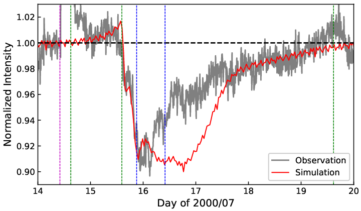
The data from observation and simulation result are presented with gray and red curves, respectively, in Figure 3 with the pre-event level of GCR intensity indicated by the black horizontal dashed line. In addition, the pink, green, and blue vertical dashed lines denote the flare onset, shock passages of the Earth, and MC boundaries, respectively. It is shown that the simulation result fits the observed decrease phase well to reproduce the two-step decrease. The pre-increase precursor of Fd, which can be found in some Fds, is also reproduced in the simulation result. From the observations and simulations we can see that the pre-increase started about 15 hours before the arrival of the shock, and the time scale is similar to the statistical result from observation, which is 10 $-$ 14 hours in average (Lingri et al. 2019). Though the observation of the pre-event GCR intensity has been contaminated by GLE59, the pre-increase in observation can be recognized roughly and is consistent with the simulation. The recovery phase of simulation, however, deviates with that of the observation during the time period between July 16 and July 18, after which the simulation is consistent with the observation again. At the end of the Fd, the observed GCR intensity was influenced by another ICME that was behind the third shock, so that the total recovery time is also affected. If the observed GCR intensity is not contaminated, it can be suggested that the total recovery time may equal to about 4 days, which is in accordance with that of simulation.

To evaluate the influence of sheath and MC, we further run simulations with only sheath or MC, with the results presented by the green and blue curves in Figure 4(a), respectively. The other curves are the same as that in Figure 3. It is shown that the simulation with only sheath, i.e., the green curve, has a sharp decrease right after the shock arrival, with an amplitude slightly larger than that of the simulation with sheath-MC, i.e., the red curve. The green curve recovers more rapidly with the total recovery time about the half of that of the red curve. The simulation with only MC, i.e., the blue curve, has a fairly rapid decrease when MC’s leading edge arrives at the Earth followed by a slow decrease lasting for about 1 day, with the smallest amplitude. Afterwards, the blue curve recovers gradually with the recovery phase in line with the red curve in the last 2.5 days. Therefore, the amplitude of Fd and the first-step decrease are mainly determined by sheath, while MC contributes to the formation of the second-step decrease and the prolonged recovery time.

The magnetic turbulence and background magnetic field are the two distinguishing features of sheath-MC structure, so their effects should be investigated. We carry out two simulations in which sheath-MC structure is included. In the first simulation the magnetic turbulence level is set according to Section IV.1 while background magnetic field is the same as that of ambient solar wind, with the result presented by the green curve in Figure 4(b). However, in the second simulation the background magnetic field is set according to Section IV.1 while magnetic turbulence level is the same as that of ambient solar wind, with the result exhibited by the blue curve in Figure 4(b). The other curves are the same as that of Figure 4(a). It is shown that the green curve has a moderate gradual decrease after the shock arrival, with the recovery time about the half of the red curve. Though the blue curve shows a two-step decrease, the amplitude of the second step decrease is too small compared to the observation. The recovery phase of the blue curve is also in line with that of the red curve in the last 2.5 days. It is shown that neither only magnetic turbulence nor background magnetic field itself can produce the observed two-step decrease. Instead, the combination of magnetic turbulence and background magnetic field in sheath-MC structure produced the two-step Fd, and the enhanced background magnetic field in sheath-MC structure extended the total recovery time.

V CONCLUSIONS AND DISCUSSION

In our previous work, WAQ-I, we use the sheath-MC model to numerically reproduce the intensity-time profiles of relatively low energy SEPs in the GLE event on 2000 July 14 successfully. It is suggested that both SEP events and Fds are two important phenomena accompanied with ICMEs, so that the results from compatible models should be consistent with both SEP and GCR observations. In this paper, as the continuation, we use the same sheath-MC model, same diffusion coefficients with magnetic turbulence as input, and similar numerical method as in WAQ-I to reproduce Fds associated with the same GLE. It is shown that there was a two-step decrease in the Oulu NM counting rates when the sheath-MC structure arrived at the Earth. we assume the two-step Fd was caused by the sheath and MC. Here, we solve the focused transport equation instead of the Parker equation since focusing effect may be large in sheath-MC structure. The simulation result is used to compare with the observed normalized intensity of GCRs measured by the Oulu NM with the effective energy as 6.54 GeV. Since Fd is a short term process and we only focus on the relative variation of GCRs, the boundary for the GCR source is set to 10 au for reducing the consumption of computing resources. Besides, the drift effect is neglected since it may have no significant influence on the formation of the two-step decrease, amplitude, and total recovery time of the Fd.

In the simulation model, the MC and sheath are set to spherical caps with fixed thickness moving in a uniform speed. The Parker field is adopted as the background magnetic field in solar wind, on which a magnetic enhancement in radial direction expressed by Equations (7) is superposed as the background magnetic field in sheath-MC structure. The magnetic turbulence levels in sheath and MC are set to higher and lower than that in ambient solar wind, respectively. The simulation result with sheath-MC structure can well reproduce the Fd event except for the first half of the recovery phase, and the two-step decrease occurs at the arrival of sheath and MC. The simulations with only one of sheath and MC infer that sheath plays an important role in the amplitude of Fd while MC contributes to the formation of the second step decrease and prolongs the recovery time of Fd. To evaluate the respective effects of magnetic turbulence and background magnetic field in sheath-MC structure on Fd, we carry out simulations with only one of the magnetic turbulent level and background magnetic field set with the ejecta model with other one set with ambient solar wind model in sheath-MC structure. The simulations show that neither the magnetic turbulence nor the background magnetic field in sheath-MC alone is sufficient to produce the observed two-step decrease in terms of the shape and amplitude of Fd. Therefore, sheath and MC and their distinguishing features, i.e., magnetic turbulence and background magnetic field are important for the formation of the two-step Fd associated with GLE59.

In this work, the input parameters of the diffusion models, i.e., the turbulence level, correlation length, and magnetic field power spectrum index are simplified. In order to be consistent with WAQ-I, recent progress in turbulence theory (Zank et al. 2018; Zhao et al. 2018; Adhikari et al. 2020; Chen et al. 2020, e.g.,), especially the radial dependence of turbulence parameters, is not included in this work. It is supposed that the simplified turbulence parameters can be used to study the Fd, which is a local and short time scale phenomenon.

In general, the simulation result with sheath-MC structure captures the main features of the observation, such as the pre-increase precursor, two-step decrease, amplitude, total recovery time, etc. However, it is shown that the simulation deviates from the observation in the first half of the recovery phase, which is reasonable due to the simplifications we make in this work. Firstly, the shapes of sheath and MC are set to thick spherical caps, which is different than the real ones. Secondly, the background magnetic field enhancement in sheath-MC structure is set in radial direction, which is different from that of the real one. In addition, the background magnetic field enhancement model we use is not divergence free. Thirdly, the drift effect, which may influence the profile of recovery phase of the Fd, is neglected. The further study can be carried out with the help of some new methods, e.g., the Grad-Shafranov reconstruction technique (Hu & Sonnerup 2002; Hu 2017) or magnetohydrodynamic (MHD) simulations (Luo et al. 2013; Pomoell & Poedts 2018; Wijsen et al. 2019; Feng 2020, e.g.,) that can produce more realistic sheath-MC structure. In addition, with the MHD simulation, which can produce a self-consistent HCS with the existence of sheath-MC structure, we can investigate the drift effect. Finally, GCRs with high energy have large gyro-radius relative to the length scale in which the background magnetic field varies significantly, so that GCRs may get into sheath-MC structure through gyromotions, and the focus transport equation based on the gyro-average of particles becomes invalid. To deal with such kind of problem in the future, we may analyze large amount of trajectories of energetic particles by numerically solving particles Newtonian equation of motion with Lorenz force in interplanetary space (Qin et al. 2002; Kong et al. 2017, e.g.,).

To evaluate the influence of the non-zero divergence, the relative divergence of the modeled background magnetic field in the Sun-Earth line is presented in Figure 5 with the blue dashed line at the time of MC arrival. In MHD simulations of solar wind, the relative divergence error of each cell in the discrete space can be defined as $\frac{|\nabla\cdot\bm{B}|}{B/R_{\text{c}}}$ (Zhang & Feng 2016, e.g.,), where $R_{\text{c}}$ is the characteristic size of the cell. The value of $R_{c}$ is about 0.01 au at 1 au, and the value is similar to that of the Larmor radius $R_{L}$ of 6.54 GeV protons at 1 au. The relative divergence error less than $10^{-2}$ is supposed small enough to simulate solar wind stably and accurately (Shen et al. 2018, e.g.,). In this work, we therefore define the relative divergence as $\frac{|\nabla\cdot\bm{B}|}{B/R_{L}}$ . Figure 5 shows that the relative divergence of the modeled background magnetic field is less than or approximately equal to $10^{-2}$ except for the sheath region. In addition, the relative gradient, defined as $\frac{|\nabla B|}{B/R_{L}}$ , is also shown in Figure 5 with the red solid line. It is shown that the relative divergence and gradient are of a similar order of magnitude. In the model of GCRs, a uniform local background magnetic field is assumed, so that the non-zero gradient introduces error in the GCR modeling. We suppose the error of the GCR modeling from non-zero divergence of magnetic field has the similar level as that from the non-zero gradient of magnetic field in sheath region.

This work was supported, in part, under grants NNSFC 41874206 and NNSFC 42074206. We thank the Wind MFI teams for providing the data used in this paper. We appreciate the availability of the Wind data at the Coordinated Data Analysis Web. The cosmic ray data were supplied by the Neutron Monitor Database (NMDB), which was founded under the European Union’s FP7 program (contract No. 213007). The work was carried out at National Supercomputer Center in Tianjin, and the calculations were performed on TianHe-1 (A).

References

Adhikari et al. (2020) Adhikari, L., Zank, G. P., Zhao, L.-L., et al. 2020, ApJS, 246, 38
Alanko et al. (2003) Alanko, K., Usoskin, I. G., Mursula, K., & Kovaltsov, G. A. 2003, AdSpR, 32, 615
Arunbabu et al. (2015) Arunbabu, K. P., Antia, H. M., Dugad, S. R., et al. 2015, A&A, 580, A41
Badruddin et al. (1986) Badruddin, Yadav, R. S., & Yadav, N. R. 1986, Sol. Phys., 105, 413
Beeck & Wibberenz (1986) Beek, J., & Wibberenz, G. 1986, ApJ, 311, 437
Bhaskar et al. (2016) Bhaskar, A., Vichare, G., Arunbabu, K. P., & Raghav, A. 2016, Ap&SS, 361, 242
Bieber et al. (1994) Bieber, J. W., Matthaeus, W. H., Smith, C. W., et al. 1994, ApJ, 420, 294
Burlaga et al. (1981) Burlaga, L., Sittler, E., Mariani, F., & Schwenn, R. 1981, J. Geophys. Res., 86, 6673
Cane (1993) Cane, H. V. 1993, J. Geophys. Res., 98, 3509
Cane (2000) Cane, H. V. 2000, Space Sci. Rev., 93, 55
Cane et al. (1997) Cane, H. V., Richardson, I. G., & Wibberenz, G. 1997, J. Geophys. Res., 102, 7075
Chen et al. (2020) Chen, C. H. K., Bale, S. D., Bonnell, J. W., et al. 2020, ApJS, 246, 53
Cocconi et al. (1958) Cocconi, G., Greisen, K., Morrison, P., Gold, T., & Hayakawa, S. 1958, NCim, 8, 161
Earl (1974) Earl, J. A. 1974, ApJ, 193, 231
Feng (2020) Feng, X. 2020, Magnetohydrodynamic Modeling of the Solar Corona and Heliosphere. (Berlin: Springer)
Firoz et al. (2019) Firoz, K. A., Gan, W. Q., Li, Y. P., Rodríguez-Pacheco, J., & Kudela, K. 2019, ApJ, 872, 178
Forbush (1937) Forbush,S. E. 1937, PhRv, 51, 1108
Gopalswamy et al. (2012) Gopalswamy, N., Xie, H., Yashiro, S., et al. 2012, Space Sci. Rev., 171, 23
Hasselmann & Wibberenz (1968) Hasselmann, K., & Wibberenz, G. 1968, ZGeo, 34, 353
Hu (2017) Hu, Q. 2017, ScChD, 60, 1466
Hu & Sonnerup (2002) Hu, Q., & Sonnerup, B. U. 2002, J. Geophys. Res., 107, 1142
Jokipii (1966) Jokippi, J. R. 1966, ApJ, 146, 480
Jordan et al. (2011) Jordan, A. P., Spence, H. E., Blake, J. B., & Shaul, D. N. A. 2011, J. Geophys. Res., 116, A11103
Kadokura & Nishida (1986) Kadokura, A., & Nishida, A. 1986, J. Geophys. Res., 91, 1
Kong et al. (2017) Kong, F. J., Qin, G., & Zhang, L. H. 2017, ApJ, 845, 43
le Roux & Potgieter (1991) le Roux, J. A., & Potgieter, M. S. 1991, A&A, 243, 531
Lepping et al. (2001) Lepping, R. P., Berdichevsky, D. B., Burlaga, L. F., et al. 2001, Sol. Phys., 204, 287
Lingri et al. (2019) Lingri, D., Mavromichalaki, H., Belov, A., et al. 2019, Sol. Phys., 294, 70
Lockwood et al. (1991) Lockwood, J. A., Webber, W. R., & Debrunner, H. 1991, J. Geophys. Res., 96, 11587
Lockwood et al. (1986) Lockwood, J. A., Webber, W. R., & Jokipii, J. R. 1986, J. Geophys. Res., 91, 2851
Luo et al. (2017) Luo, X., Potgieter, M. S., Zhang, M., & Feng, X. 2017, ApJ, 839, 53
Luo et al. (2018) Luo, X., Potgieter, M. S., Zhang, M., & Feng, X. 2018, ApJ, 860, 160
Luo et al. (2013) Luo, X., Zhang, M., Rassoul, H. K., et al. 2013, ApJ, 764, 85
Matthaeus et al. (1990) Matthaeus, W. H., Goldstein, M. L., & Roberts, D. A. 1990, J. Geophys. Res., 95, 20673
Matthaeus et al. (2003) Matthaeus, W. H., Qin, G., Bieber, J. W., & Zank, G. P. 2003, ApJ, 590, L53
Melkumyan et al. (2019) Melkumyan, A., Belov, A., Abunina, M., et al. 2019, Journal of Physics: Conference Series, 1181, 012009
Mewaldt et al. (2012) Mewaldt, R. A., Looper, M. D., Cohen, C. M. S., et al. 2012, Space Sci. Rev., 171, 97
Morrison (1956) Morrison, P. 1956, PhRv, 101, 1397
Mulder & Moraal (1986) Mulder, M. S., & Moraal, H. 1986, ApJ, 303, L75
Nishida (1982) Nishida, A. 1982, J. Geophys. Res., 87, 6003
Parker (1965) Parker, E. N. 1965, Planet. Space Sci., 13, 9
Piddington (1958) Piddington, J. H. 1958, PhRv, 112, 589
Pomoell & Poedts (2018) Pomoell, J., & Poedts, S. 2018, JSWSC, 8, A35
Potgieter et al. (2014) Potgieter, M. S., Vos, E. E., Boezio, M., et al. 2014, Sol. Phys., 289, 391
Qin et al. (2002) Qin, G., Matthaeus, W. H., & Bieber, J. W. 2002, ApJ, 578, L117
Qin & Shen (2017) Qin, G., & Shen, Z.-N. 2017, ApJ, 846, 56
Qin et al. (2006) Qin, G., Zhang, M., & Dwyer, J. R. 2006, J. Geophys. Res., 111, A08101
Rana et al. (1996) Rana, D. S., Sharma, N. K., & Yadav, R. S. 1996, Sol. Phys., 167, 371
Richardson & Cane (2010) Richardson, I. G., & Cane, H. V. 2010, Sol. Phys., 264, 189
Richardson & Cane (2011) Richardson, I. G., & Cane, H. V. 2011, Sol. Phys., 270, 609
Richardson et al. (1999) Richardson, I. G., Cane, H. V., & Cyr, O. C. St. 1999, AIP Conference Proceedings, 471, 677
Sanderson et al. (1990) Sanderson, R. T., Beeck, J., Marsden, G. R., et al. 1990, Proceedings of the 21st International Cosmic Ray Conference, 6, 251
Schlicheiser (2002) Schlicheiser, R. 2002, Cosmic Ray Astrophysics (Berlin: Springer)
Shaikh et al. (2017) Shaikh, Z., Raghav, A., & Bhaskar, A. 2017, ApJ, 844, 121
Shalchi et al. (2004) Shalchi, A., Bieber, J. W., Matthaeus, W. H., & Qin, G. 2004, ApJ, 616, 617
Shalchi et al. (2010) Shalchi, A., Li, G., & Zank, G. P. 2010, Ap&SS, 325, 99
Shen et al. (2018) Shen, F., Yang, Z., Zhang, J., Wei, W., & Feng X. 2018, ApJ, 866, 18
Shen & Qin (2018) Shen, Z.-N., & Qin, G. 2018, ApJ, 854, 137
Shen et al. (2019) Shen, Z.-N., Qin, G., Zuo, P., & Wei, F. 2019, ApJ, 887, 132
Simpson (1954) Simpson, J. A. 1954, PhRv, 94, 426
Singh & Badruddin (2006) Singh, Y. P., & Badruddin. 2006, Sol. Phys., 234, 339
Skilling (1971) Skilling, J. 1971, ApJ, 170, 265
Teufel & Schlickeiser (2003) Teufel, A., & Schlickeiser, R. 2003, A&A, 397, 15
Thomas & Gall (1984) Thomas, B. T., & Gall, R. 1984, J. Geophys. Res., 89, 2991
Wawrzynczak & Alania (2008) Wawrzynczak, A., & Gall, M. V. 2008, AdSpR, 41, 325
Weygand et al. (2009) Weygand, J. M., Matthaeus, W. H., Dasso, S., & Kivelson, M. G. 2009, J. Geophys. Res., 114, A07213
Weygand et al. (2011) Weygand, J. M., Matthaeus, W. H., Dasso, S., & Kivelson, M. G. 2011, J. Geophys. Res., 116, A08102
Wijsen et al. (2019) Wijsen, N., Aran, A., Pomoell, J., & Poedts, S. 2019, A&A, 622, A28
Wu & Qin (2018) Wu, S.-S., & Qin, G. 2018, J. Geophys. Res.: Space Physics, 123, 76
Wu & Qin (2020) Wu, S.-S., & Qin, G. 2020, ApJ, 904, 151
Yu et al. (2010) Yu, X. X., Lu, H., Le, G. M., & Shi, F. 2010, Sol. Phys., 263, 223
Zank et al. (2018) Zank, G. P., Adhikari, L., Zhao, L.-L., et al. 2018, ApJ, 869, 23
Zhang & Burlaga (1988) Zhang, G., & Burlaga, L. F. 1988, J. Geophys. Res., 93, 2511
Zhang (1999) Zhang, M. 1999, ApJ, 513, 409
Zhang & Feng (2016) Zhang, M., & Feng, X. 2016, FrASS, 3, 1
Zhang et al. (2009) Zhang, M., Qin, G., & Rassoul, H. 2009, ApJ, 692, 109
Zhang et al. (2019) Zhang, M., Zhao, L., & Rassoul, H. K. 2019, Journal of Physics: Conference Series, 1225, 012010
Zhao et al. (2014) Zhao, L.-L., Qin, G., Zhang, M., & Heber, B. 2014, J. Geophys. Res.: Space Physics, 119, 1493
Zhao et al. (2018) Zhao, L.-L., Adhikari, L., Zank, G. P., Hu, Q., & Feng, X. S. 2018, ApJ, 856, 94

Refer to caption — Figure 1: Observations for the Fd associated with GLE59. (a) The normalized intensity of GCR measured by the Oulu NM is plotted with the black solid curve, and the pre-event level is presented with the black horizontal dashed line. The pink and green vertical dashed lines denote flare onset and the passages of ICME shock, respectively. The boundaries of ICME and MC are presented with the red and blue vertical solid lines, respectively. (b) $-$ (d) are the intensity, polar angle, and azimuthal angle of IMF provided by Wind spacecraft in GSE angular coordinates, respectively.

Table 1: Parameter settings for the simulation.

Type	Parameter	Meaning	Value
Shock	$v_{\text{s}}$	speed	1406 km/s
Shock	$\Omega_{\text{s}}$	half angular width	$45^{\circ}$
Solar wind	$V^{\text{sw}}$	speed	450 km/s
	$B_{\text{P}0}$	radial strength of IMF at 1 au	3.62 nT
	$B_{\text{P}}\|_{1\text{au}}$	total strength of IMF at 1 au	5 nT
MC	$L_{\text{M}}$	half thickness	0.22 au
MC	$d_{\text{M}}$	distance between MC center and shock	0.45 au
Sheath	$L_{\text{S}}$	half thickness	0.08 au
Others	$\omega$	angular speed of solar rotation	2 $\pi$ /25.4 rad/day
	$R_{\text{in}}$	inner boundary	0.05 au
	$R_{\text{out}}$	outer boundary	10 au
	$E_{\text{eff}}$	effective energy of Oulu NM	6.54 GeV

Table 2: Parameter settings of turbulence for the simulation.

Parameter		Meaning	Value
$\sigma_{\text{P}}$		turbulence level in solar wind	0.3
$\sigma_{\text{ejecta}}$	$\sigma_{\text{S}}$	turbulence level in sheath	1.6
$\sigma_{\text{ejecta}}$	$\sigma_{\text{M}}$	turbulence level in MC	0.1
$l_{\text{turb}}$	$l_{\text{slab}}$	slab correlation length	0.025 au
$l_{\text{turb}}$	$l_{\text{2D}}$	2D correlation length	0.0096 au
$s$		Kolmogorov spectral index	$5/3$
$h$		non-linear effect index	$0.01$