Spontaneous Leptogenesis in Higgs Inflation

Higgs inflation has attracted a lot of attention due to its simplicity and consistency to the current measurement of the spectral index $n_{s}$ and tensor-to-scalar ratio $r$. To suppress $r$ value, one introduces a non-minimal coupling between the Higgs scalar and the Ricci scalar $R$. One of the distinguished features of the Higgs inflation is that the fermion masses are very large and time-dependent during the inflation and subsequent reheating epochs due to the dynamics of the vacuum expectation value of the Higgs field as an inflaton. We emphasize that this is also responsible for the large lepton asymmetry generated from the Higgs inflaton condensate.³³ 3 See Ref. Pearce:2015nga where lower reheating temperature of the order of $10^{12}~\rm GeV$ is assumed in order to generate sufficient lepton number to photon ratio in a non-Higgs inflation. In Ref. Enomoto:2020lpf oscillating Higgs field during (p)reheating is considered with preexisting C/CP violation as the source of asymmetry.

In addition, to describe the action in the canonical Einstein frame without the non-minimal coupling, one performs the conformal transformation. From this, fermion masses also obtain additional conformal weight. See Appendix A for detailed derivation.

The Jordan-frame action of the inflaton sector is given by the SM Higgs with a non-minimal coupling constant $\xi$:

where $J$ stands for the Jordan frame, $V_{J}(\phi_{J})=\frac{\lambda}{4}\phi_{J}^{4}$, and the real scalar $\phi_{J}$ is the physical Higgs direction in the unitary gauge. We transform the action Eq. (2) to Einstein frame with Weyl transformation:

where we truncate the conformal factor $\Omega^{2}$ up to the quadratic power of $\phi_{J}$:

We have omitted explicit $E$ subscript for simplicity. The final form of the action in the Einstein frame is

where the potential in the Einstein frame $V(\phi)$ is

The inflaton fields in both frames are related by

In the limit of $\xi\phi\gg M_{P}$, Eq. (4) and Eq. (7) can be approximated as

Therefore,

Let $\phi_{0}$ be the inflaton field value at the end of inflation, after which the inflaton potential can be approximated by a quadratic form in general:⁴⁴ 4 This approximation to quadratic potential form is generically valid in Higgs inflation when $\frac{M_{P}}{\xi}\ll\phi\lesssim\frac{M_{P}}{\sqrt{\xi}}$, corresponding to early stages of the reheating where the amplitude of oscillation is in intermediate range. The value of $\phi$ stays large ($\phi\gg M_{P}/\xi$) most of the time, and passes by smaller field value regime only in short periods of time. After several oscillations the amplitude becomes small $\phi\mathrel{\hbox to0.0pt{\lower 4.0pt\hbox{\hskip 1.0pt$\sim$}\hss}\raise 1.0pt\hbox{$<$}}M_{P}/\xi$ and the potential is reduced to the conventional quartic one in lower energies. More details are found in Appendix A.

Here, $M$ determines the frequency of the oscillation right after the inflation. Then the solution of the Friedmann equations

describes the dynamics of the oscillating homogeneous inflaton field as an approximate form Kofman:1997yn

In the Higgs inflation, the effective mass $M$ during the oscillation is not a free parameter but fixed from $\lambda$ and $\xi$ as $M^{2}=\frac{\lambda M_{P}^{2}}{3\xi^{2}}$, and $\phi_{0}$ is order of Planck scale GarciaBellido:2008ab. As we will see, the neutrino mass and the effective chemical potential of lepton number change in time accordingly to the oscillating Higgs field in Eq. (13).

In the SM, it is the simplest to introduce the Weinberg operator, the minimal lepton-number-violating dimension-five operator, in order to account for the observed neutrino masses:

where $\widetilde{\Phi}\equiv i\sigma_{2}\Phi^{*}$ and we have assumed this operator is Planck suppressed with a parameter $c_{5}\lesssim\mathcal{O}(1)$. This can be used to realize a leptogenesis. We emphasize that we are in the Jordan frame now. Although we will only consider a single flavor in the following discussion, the generalizations to three flavor or more are straightforward.

This operator generates the neutrino mass

in Einstein frame, where we take conformal transformation of the fermion mass $m\rightarrow m/\Omega$ into account. The detailed derivation of Eq. (15) is found in Appendix A.

On the other hand, during and right after the inflation, the fact that the inflaton field is nearly homogeneous implies $\partial_{\mu}\phi=\dot{\phi}\delta_{\mu}^{0}$. As mentioned in Introduction, this inflaton background spontaneously breaks Lorentz symmetry, and hence CPT symmetry. We emphasize that this is universal characteristic of all standard inflation scenarios and motivates us to think the spontaneous symmetry breaking of CPT as the source of matter-antimatter asymmetry in the inflationary framework.

As we will see, when inflaton couples to derivative of a lepton (or baryon) current $j_{L}^{\mu}=\overline{\ell}\sigma^{\mu}\ell$, the CPT breaking actually leads to asymmetry between decay rates into particles and antiparticles. In this work, we introduce an effective dimension-six operator Pearce:2015nga:

where we have taken unitary gauge to the Higgs doublet $\Phi$ and the dimensionless constant $c_{6}$ parameterizes the size of the dimension-six effective coupling. In the last equation, we used the spatial homogeneity of the inflaton sector. $j_{L}^{0}$ has the meaning of the number density of the lepton, $j_{L}^{0}\equiv n_{L}=l^{\dagger}l=n_{\ell}-n_{\overline{\ell}}$. Note that the operator Eq. (16) does not violate the lepton number by itself, though it generate a difference of decay rates between particles and anti-particles under presence of another lepton-number violating operator. Therefore, we introduce explicit lepton number violating Weinberg operator as discussed earlier.⁵⁵ 5 However, there is another source of lepton number violation in Eq. (16): anomalous $B+L$. In general, the global $L$ is anomalous and its current $j^{\mu}_{L}$ is not conserved. Indeed in the SM, what is anomalous is $B+L$, and therefore the anomaly-induced higher-dimensional operator from $\Phi^{\dagger}\Phi F\widetilde{F}$ should rather be $\Phi_{J}^{\dagger}\Phi_{J}\partial_{\mu}(j_{L}^{\mu}+j_{B}^{\mu})$. Without additional source of $B-L$ breaking, the generated $B+L$ by this operator would be quickly washed out by the sphaleron effects in the absence of strong first order phase transition.

A possible intuitive interpretation of the operator Eq. (16) is as an effective chemical potential in the sense that this term makes energy density shift, $\Delta\rho=-\frac{c_{6}}{M_{P}^{2}}(\partial_{t}\phi^{2})j_{L}^{0}$ Cohen:1987vi; Cohen:1988kt; DeSimone:2016ofp, although this picture is under controversy; see Refs. Dolgov:1996qq; Dasgupta:2018eha. Note that our result of asymmetry between particle and anti-particle is valid no matter whether this interpretation is possible or not. Anyway motivated by this interpretation, we call the following the “(effective) chemical potential”:

As we will see, this makes difference between dispersion relations of particle and antipaticle. Due to the exact cancellation of the conformal factor from the metric and current, the effective chemical potential does not obtain additional conformal factor. However, we still need to consider the inflaton field transformation

Fig. 1 shows shape of the chemical potential and the neutrino mass as a function of the number of oscillations.

In the oscillating phase, the Higgs field varies in time and results in oscillations of SM particle masses, especially of neutrino ones that are induced by lepton number violating Weinberg operator in Eq. (15). The generated numbers of neutrinos and anti-neutrinos can be obtained by a method analogous to the gravitational particle production in time dependent background Birrell:1982ix; Mukhanov:2007zz following Ref. Pearce:2015nga. The details of calculations are found in Appendix B, and we only briefly sketch the ideas and some key results here.

The equation of motion for neutrino with the chemical potential term in Eq. (16) in momentum space is:

Here we use the conformal time defined as $\tau\equiv\int dt/a(t)$ and the comoving momentum $k\equiv ap$, and mass parameters $\widetilde{m}_{\nu}\equiv am_{\nu}$ and $\widetilde{\mu}\equiv a\mu$ with $a$ and $p$ being the scale factor and the physical momentum, respectively. We also define time derivatives as $F^{\prime}\equiv\partial_{\tau}F$ and $\dot{F}\equiv\partial_{t}F$ for any function $F$.

By Bogoliubov transformation, Eq. (19) leads to a coupled equations of Bogoliubov coefficients $\alpha$ and $\beta$,

with the initial conditions $\alpha_{s}(0,k)=1$ and $\beta_{s}(0,k)=0$, where $s=\pm$ represents helicity states. These equations are numerically solved from $\tau=0$ at the end of the inflation. Importantly, non-zero $\beta_{s}$ values at late times indicate particle production from the time dependent background: the generated number density for the helicity $s$ is given by

where $\beta_{s}(\tau,k)$ is Bogoliubov coefficient from the time-dependent background or the change of vacuum state at each moment obtained by Eq. (3.1) and $a_{\rm end}$ is the scale factor at the end of the inflation. Note that $a(t)^{-3}$ factor in front accounts dilution from the expansion of the universe. The occupation number for $s$ at the end of reheating is $f_{s}(t,k)=|\beta_{s}(\tau(t),k)|^{2}$. The final net number density of the produced lepton is the difference between the number densities of each helicity states at a sufficiently late time when the Higgs field value becomes small so that $m_{\nu}(\phi)\ll T_{\rm reh}$ Pearce:2015nga:

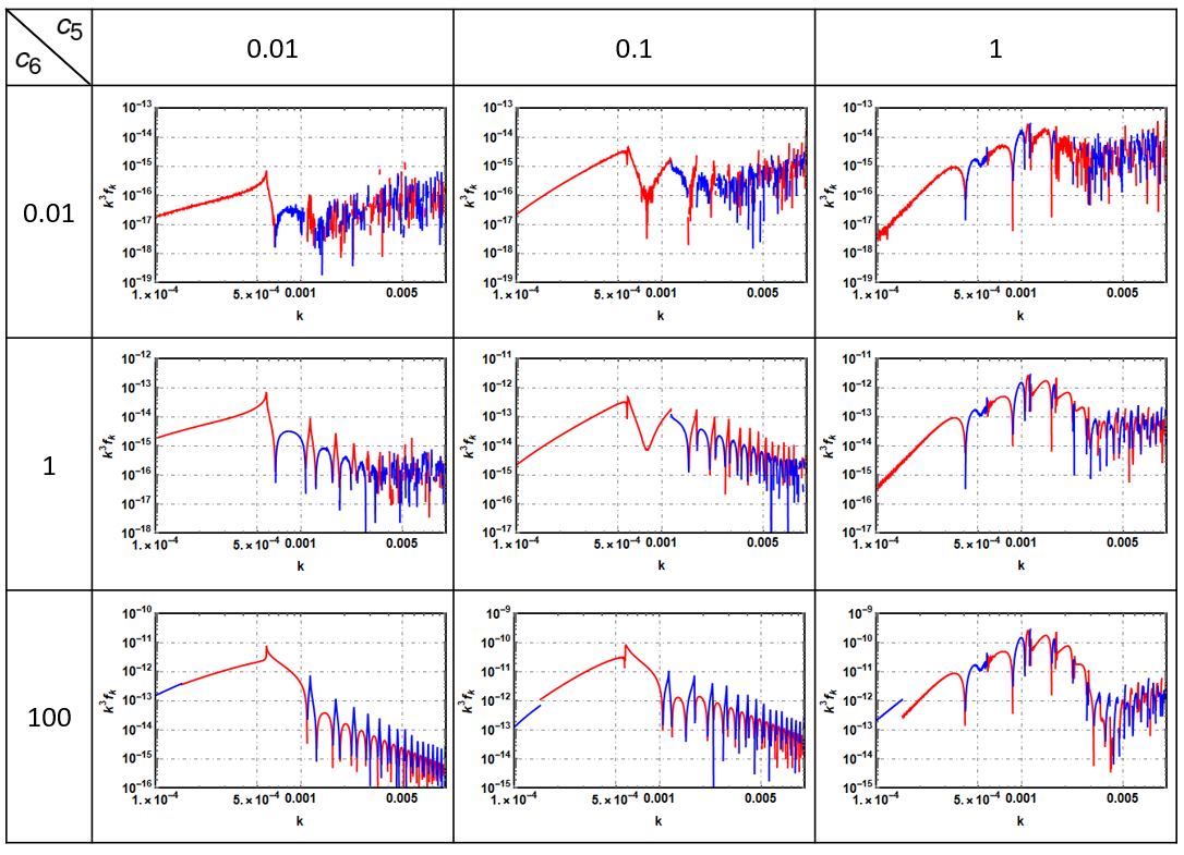
where the net occupation number is the helicity weighted sum at the end of the reheating $f(p)=f(t_{\rm reh},k)=\sum_{s}sf_{s}(k)=f_{+}-f_{-}$ describing the differences between particle ($s=+$) and anti-particle ($s=-$). Comoving lepton number density $\widetilde{n}_{L}\equiv\int\frac{d^{3}k}{(2\pi)^{3}}f(k)$ is insensitive to $t_{\rm reh}$ as $f(t,k)$ rapidly approches to a constant for a given $k$. The explicit evolution of the occupation numbers $f(t,k)$ for various modes are depicted in Fig. 2. Note that the asymmetry is dominantly generated during the early time within first several oscillations so that it is relatively insensitive to exact value of $t_{\rm reh}$. $\widetilde{n}_{L}$ is determined by $c_{5}$ and $c_{6}$ paramters. Final spectrum of the occupation number $f(k)$ multiplied by $k^{3}$ taking the contribution from the phase space are also shown in Fig. 3. For large $k$ modes, the occupation numbers are suppressed. For small modes, even though the occupation numbers are larger, the phase space is too small to contribute to the final asymmetry.

Finally, the lepton asymmetry is given by

where the photon number density at the end of the reheating ${n_{\gamma}|_{\rm reh}=\frac{2\zeta(3)}{\pi^{2}}T_{\rm reh}^{3}}$ with $\zeta(3)\simeq 1.2$ and $\widetilde{T}\equiv e^{N_{\rm reh}}T_{\rm reh}$ where $N_{\rm reh}=\ln\left(\frac{a_{\rm reh}}{a_{\rm end}}\right)$.⁶⁶ 6 Because the interaction rate due to the dimension-five operator 14 is small compared to the expansion rate, there will be no further lepton number production after the reheating. When we regard Majorana neutrino as the origin of dimension-five operator, this is equivalent to impose $T_{\rm reh}<M_{N}$, which is satisfied in Higgs inflation when $M_{N}\gtrsim\mathcal{O}(10^{15}~\rm GeV)$. See Figure 4. Because $\widetilde{n}_{L}$ is solely determined by $c_{5}$ and $c_{6}$, it suffices to specify $\widetilde{T}$ (which we call ‘rescaled temperature’) to obtain $\eta_{L}(t_{\rm reh})$. Although (p)reheating processes after the end of inflation is highly non-trivial and model dependent,⁷⁷ 7 Early analysis relevant for the reheating in the Higgs inflation is done in Refs. Bezrukov:2008ut; GarciaBellido:2008ab; Repond:2016sol; DeCross:2015uza. For the possible unitarity violation issue during the Higgs inflation reheating, see Refs. Ema:2016dny; Hamada:2020kuy. In particular, Ref. Ema:2016dny argued that the longitudinal mode of gauge boson production is so violent that preheating may finish right after the first oscillation in Higgs inflation with a large non-minimal coupling $\xi\gtrsim 100$. However, this phenomena violates the unitarity but also is sensitive to higher order operators Hamada:2020kuy. Therefore, we will assume there are at least a few oscillations after the inflation in our work. we can find possible parameter regions of the rescaled temperature without large uncertainties Cook:2015vqa as we will see below. See Appendix C for more detailed review.

Rescaled temperature $\widetilde{T}\equiv e^{N_{\rm reh}}T_{\rm reh}$ can be inferred by the Hubble scale $H_{*}$ at pivot scale and e-folding number $N_{*}$ between time when the pivot scale $k_{*}$ crosses the horizon and the time at the end of the inflation without the knowledge of the equation of state during the reheating:

For a given model of inflation, $H_{*}$ and $N_{*}$ are generally related to the slow-roll parameters $\epsilon$ and $\eta$, hence the observables $n_{s}$ and $r$ at pivot scale. In the case of Higgs inflation Bezrukov:2007ep,

The Hubble scale also determines the amplitude of the power spectrum is given by

Hence, we can evaluate $\widetilde{T}$ solely as a function of $n_{s}$. Fig. 4 depicts the values of $\widetilde{T}$ and $T_{\rm reh}$ as a function of the spectral index $n_{s}$. Note that rescaled temperature $\widetilde{T}$ is independent of equation of state, $w=p/\rho$ during the reheating while $T_{\rm reh}$ itself is highly depends on $w$ Gong:2015qha; Cai:2015soa; Cook:2015vqa. From the Planck 2018 1$\sigma$ bound, we will consider $\widetilde{T}\in(10^{15}-10^{18}){\rm GeV}$ as a preferred regime. Assuming $w=0$, the reheating temperature suggested in Ref. Bezrukov:2008ut $T_{\rm reh}\in(3\times 10^{13}-1.5\times 10^{14})~\rm GeV$ corresponds to $\widetilde{T}\simeq 10^{16}~\rm GeV$, which is also within the preferred regime.

In our scenario, ‘net’ $B-L$ number (in fact, only $L$ number) is generated right after the inflation and is frozen by the time of the end of reheating. Later, generated lepton number asymmetry transfers to baryon number through sphaleron effects, conserving $B-L$, so that

Khlebnikov:1988sr. Therefore, for successful baryon asymmetry, we also require $\eta_{L,i}\gtrsim 3\eta_{B}$.

Considering the transition through the sphaleron effect, final baryon asymmetry for given comoving lepton number $\widetilde{n}_{L}(c_{5},c_{6})$ and rescaled reheating temperature $\widetilde{T}$ is given by

The observed value is $\eta_{B,\rm obs}\simeq 6\times 10^{-10}$ Zyla:2020zbs. As can be seen from Fig. 5, there exist reasonable parameter regions of ($c_{5},c_{6}$) and $(\lambda,\xi)$ in the Higgs inflation scenario which explain current baryon asymmetry $\eta_{B}$ with desired rescaled temperature.

To avoid unitarity violation from larger $m_{\nu}$ or $\mu_{\rm eff}$ than cut-off scale of Higgs inflation during the reheating $\Lambda=M_{P}/\xi$ Burgess:2009ea; Barbon:2009ya; Burgess:2010zq; Lerner:2009na; Bezrukov:2010jz, we will only consider the cases where $c_{5}\lesssim 1$ and $c_{6}\lesssim 100$. The particles with the momentum larger than the cut-off would be strongly coupled and their behavior cannot be descibed within the effective field theory. In our parameter choice, the majority of the particles are generated with momentum smaller than the cut-off scale $\Lambda=M_{P}/\xi$ as depicted in Fig. 3.⁸⁸ 8 In Fig. 3, the Einstein-frame momentum cut-off is $\Lambda=M_{P}/\xi=0.01$. Large $c_{6}\sim 100$ makes it one order of magnitude smaller, $\Lambda/\sqrt{c_{6}}\sim 10^{-3}$. We see that the unitarity issue arises, namely the location of dominant peaks becomes located at $p\gtrsim 10^{-3}$, only when $c_{5}\gtrsim 1$ and $c_{6}\gtrsim 100$. For larger $\xi\gtrsim 10^{4}$, the suppression on lepton number density so large that the asymmetry may not be enough to explain current relic within preferred temperature regime. This can be seen in Fig. 5.

Usually, it is believed that the spontaneous baryogenesis mechanism does not work in super-cooled regime due to its inefficiency from the cancellation during the oscillations DeSimone:2016ofp. However, as identifying the inflaton decay as the source of the lepton asymmetry, both the amplitude of the effective chemical potential and the neutrino mass are so large that the produced lepton numbers are enough to explain current relic density without any fine-tuning of the parameters. We also do not have to assume such a low scale inflation as in Ref. Pearce:2015nga, which considers neutrino decay from the condensate of the SM Higgs (not identified as the inflaton).

As the final remark, we note that the strong bound on spontaneous baryogenesis from baryon isocurvature perturbation DeSimone:2016ofp is not imposed in our scenario because we do not assume any light bosonic fields in the early time other than SM. This is one of the advantages regarding the possibility of the inflaton decay as the source of baryon asymmetry.

References

- (1) A. Sakharov, “Violation of CP Invariance, C asymmetry, and baryon asymmetry of the universe,” Sov. Phys. Usp. 34 no. 5, (1991) 392–393.
- (2) Particle Data Group Collaboration, P. Zyla et al., “Review of Particle Physics,” PTEP 2020 no. 8, (2020) 083C01.
- (3) M. Fukugita and T. Yanagida, “Baryogenesis Without Grand Unification,” Phys. Lett. B174 (1986) 45–47.
- (4) S. Davidson, E. Nardi, and Y. Nir, “Leptogenesis,” Phys. Rept. 466 (2008) 105–177, arXiv:0802.2962 [hep-ph].
- (5) S. Blanchet and P. Di Bari, “The minimal scenario of leptogenesis,” New J. Phys. 14 (2012) 125012, arXiv:1211.0512 [hep-ph].
- (6) D. Bodeker and W. Buchmuller, “Baryogenesis from the weak scale to the GUT scale,” arXiv:2009.07294 [hep-ph].
- (7) S. Khlebnikov and M. Shaposhnikov, “The Statistical Theory of Anomalous Fermion Number Nonconservation,” Nucl. Phys. B 308 (1988) 885–912.
- (8) E. J. Chun, K. Y. Lee, and S. C. Park, “Testing Higgs triplet model and neutrino mass patterns,” Phys. Lett. B566 (2003) 142–151, arXiv:hep-ph/0304069 [hep-ph].
- (9) Y. Jho and S. C. Park, “Constraining New Physics with High Multiplicity : I. Ultra-High Energy Cosmic Rays on air-shower detector arrays,” arXiv:1806.03063 [hep-ph].
- (10) A. G. Cohen and D. B. Kaplan, “Thermodynamic Generation of the Baryon Asymmetry,” Phys. Lett. B 199 (1987) 251–258.
- (11) A. G. Cohen and D. B. Kaplan, “SPONTANEOUS BARYOGENESIS,” Nucl. Phys. B 308 (1988) 913–928.
- (12) A. Dolgov and K. Freese, “Calculation of particle production by Nambu Goldstone bosons with application to inflation reheating and baryogenesis,” Phys. Rev. D 51 (1995) 2693–2702, arXiv:hep-ph/9410346.
- (13) A. Dolgov, K. Freese, R. Rangarajan, and M. Srednicki, “Baryogenesis during reheating in natural inflation and comments on spontaneous baryogenesis,” Phys. Rev. D 56 (1997) 6155–6165, arXiv:hep-ph/9610405.
- (14) F. Takahashi and M. Yamada, “Spontaneous Baryogenesis from Asymmetric Inflaton,” Phys. Lett. B 756 (2016) 216–220, arXiv:1510.07822 [hep-ph].
- (15) V. Domcke, Y. Ema, K. Mukaida, and M. Yamada, “Spontaneous Baryogenesis from Axions with Generic Couplings,” JHEP 08 (2020) 096, arXiv:2006.03148 [hep-ph].
- (16) N. D. Barrie, A. Sugamoto, T. Takeuchi, and K. Yamashita, “Higgs Inflation, Vacuum Stability, and Leptogenesis,” JHEP 08 (2020) 072, arXiv:2001.07032 [hep-ph].
- (17) D. Salopek, J. Bond, and J. M. Bardeen, “Designing Density Fluctuation Spectra in Inflation,” Phys. Rev. D 40 (1989) 1753.
- (18) F. L. Bezrukov and M. Shaposhnikov, “The Standard Model Higgs boson as the inflaton,” Phys. Lett. B 659 (2008) 703–706, arXiv:0710.3755 [hep-th].
- (19) S. Weinberg, “Baryon- and lepton-nonconserving processes,” Phys. Rev. Lett. 43 (Nov, 1979) 1566–1570. https://link.aps.org/doi/10.1103/PhysRevLett.43.1566.
- (20) L. Kofman, A. D. Linde, and A. A. Starobinsky, “Towards the theory of reheating after inflation,” Phys. Rev. D 56 (1997) 3258–3295, arXiv:hep-ph/9704452.
- (21) J. Garcia-Bellido, D. G. Figueroa, and J. Rubio, “Preheating in the Standard Model with the Higgs-Inflaton coupled to gravity,” Phys. Rev. D 79 (2009) 063531, arXiv:0812.4624 [hep-ph].
- (22) F. Bezrukov, D. Gorbunov, and M. Shaposhnikov, “On initial conditions for the Hot Big Bang,” JCAP 06 (2009) 029, arXiv:0812.3622 [hep-ph].
- (23) L. Pearce, L. Yang, A. Kusenko, and M. Peloso, “Leptogenesis via neutrino production during Higgs condensate relaxation,” Phys. Rev. D 92 no. 2, (2015) 023509, arXiv:1505.02461 [hep-ph].
- (24) S. Enomoto, C. Cai, Z.-H. Yu, and H.-H. Zhang, “Leptogenesis due to oscillating Higgs field,” arXiv:2005.08037 [hep-ph].
- (25) A. De Simone and T. Kobayashi, “Cosmological Aspects of Spontaneous Baryogenesis,” JCAP 08 (2016) 052, arXiv:1605.00670 [hep-ph].
- (26) A. Dasgupta, R. K. Jain, and R. Rangarajan, “Effective chemical potential in spontaneous baryogenesis,” Phys. Rev. D 98 no. 8, (2018) 083527, arXiv:1808.04027 [hep-ph].
- (27) N. Birrell and P. Davies, Quantum Fields in Curved Space. Cambridge Monographs on Mathematical Physics. Cambridge Univ. Press, Cambridge, UK, 2, 1984.
- (28) V. Mukhanov and S. Winitzki, Introduction to quantum effects in gravity. Cambridge University Press, 6, 2007.
- (29) J. Repond and J. Rubio, “Combined Preheating on the lattice with applications to Higgs inflation,” JCAP 07 (2016) 043, arXiv:1604.08238 [astro-ph.CO].
- (30) M. P. DeCross, D. I. Kaiser, A. Prabhu, C. Prescod-Weinstein, and E. I. Sfakianakis, “Preheating after Multifield Inflation with Nonminimal Couplings, I: Covariant Formalism and Attractor Behavior,” Phys. Rev. D 97 no. 2, (2018) 023526, arXiv:1510.08553 [astro-ph.CO].
- (31) Y. Ema, R. Jinno, K. Mukaida, and K. Nakayama, “Violent Preheating in Inflation with Nonminimal Coupling,” JCAP 02 (2017) 045, arXiv:1609.05209 [hep-ph].
- (32) Y. Hamada, K. Kawana, and A. Scherlis, “On Preheating in Higgs Inflation,” arXiv:2007.04701 [hep-ph].
- (33) J. L. Cook, E. Dimastrogiovanni, D. A. Easson, and L. M. Krauss, “Reheating predictions in single field inflation,” JCAP 04 (2015) 047, arXiv:1502.04673 [astro-ph.CO].
- (34) Planck Collaboration, Y. Akrami et al., “Planck 2018 results. X. Constraints on inflation,” arXiv:1807.06211 [astro-ph.CO].
- (35) J.-O. Gong, S. Pi, and G. Leung, “Probing reheating with primordial spectrum,” JCAP 05 (2015) 027, arXiv:1501.03604 [hep-ph].
- (36) R.-G. Cai, Z.-K. Guo, and S.-J. Wang, “Reheating phase diagram for single-field slow-roll inflationary models,” Phys. Rev. D 92 (2015) 063506, arXiv:1501.07743 [gr-qc].
- (37) C. P. Burgess, H. M. Lee, and M. Trott, “Power-counting and the Validity of the Classical Approximation During Inflation,” JHEP 09 (2009) 103, arXiv:0902.4465 [hep-ph].
- (38) J. L. F. Barbon and J. R. Espinosa, “On the Naturalness of Higgs Inflation,” Phys. Rev. D79 (2009) 081302, arXiv:0903.0355 [hep-ph].
- (39) C. P. Burgess, H. M. Lee, and M. Trott, “Comment on Higgs Inflation and Naturalness,” JHEP 07 (2010) 007, arXiv:1002.2730 [hep-ph].
- (40) R. N. Lerner and J. McDonald, “Higgs Inflation and Naturalness,” JCAP 1004 (2010) 015, arXiv:0912.5463 [hep-ph].
- (41) F. Bezrukov, A. Magnin, M. Shaposhnikov, and S. Sibiryakov, “Higgs inflation: consistency and generalisations,” JHEP 01 (2011) 016, arXiv:1008.5157 [hep-ph].
- (42) Y. Hamada, H. Kawai, K.-y. Oda, and S. C. Park, “Higgs Inflation Still Alive,” Phys. Rev. Lett. 112 no. 24, (2014) 241301, arXiv:1403.5043 [hep-ph].
- (43) F. Bezrukov and M. Shaposhnikov, “Higgs inflation at the critical point,” Phys. Lett. B 734 (2014) 249–254, arXiv:1403.6078 [hep-ph].
- (44) Y. Hamada, H. Kawai, K.-y. Oda, and S. C. Park, “Higgs inflation from Standard Model criticality,” Phys. Rev. D 91 (2015) 053008, arXiv:1408.4864 [hep-ph].