2021
Dynamic Walking:
Toward Agile and Efficient Bipedal Robots
Journal: Annu. Rev. Control Robot. Auton. SystDOI: 10.1146/DOI
Abstract
Dynamic walking on bipedal robots has evolved from an idea in science fiction to a practical reality. This is due to continued progress in three key areas: a mathematical understanding of locomotion, the computational ability to encode this mathematics through optimization, and the hardware capable of realizing this understanding in practice. In this context, this review article outlines the end-to-end process of methods which have proven effective in the literature for achieving dynamic walking on bipedal robots. We begin by introducing mathematical models of locomotion, from reduced order models that capture essential walking behaviors to hybrid dynamical systems that encode the full order continuous dynamics along with discrete footstrike dynamics. These models form the basis for gait generation via (nonlinear) optimization problems. Finally, models and their generated gaits merge in the context of real-time control, wherein walking behaviors are translated to hardware. The concepts presented are illustrated throughout in simulation, and experimental instantiation on multiple walking platforms are highlighted to demonstrate the ability to realize dynamic walking on bipedal robots that is agile and efficient.
keywords
robotics, control theory, optimization, hybrid systems, bipedal robots, dynamic walking1 INTRODUCTION
The realization of human-like capabilities on artificial machines has captured the imagination of humanity for centuries. The earliest attempts to realize this were through purely mechanical means. In , Leonardo da Vinci detailed his Automa cavaliere, a primitive humanoid in a knights armor and operated by a number of pulleys and cables. However, these mechanical automatons lacked the ability to apply feedback control and thus the field remained largely dormant until digital computers became broadly available. In the word “robot” was coined by Czech playwriter Karel Carek, just years before microprocessors were introduced and soon thereafter the field of legged robots began to emerge.
Today, the field of robotic legged locomotion is of special interest to researchers as humans increasingly look to augment their natural environments with intelligent machines. In order for these robots to navigate the unstructured environments of the world and perform tasks, they must have the capability to reliably and efficiently locomote. The first control paradigms for robotic walking used a notion of static stability where the vertical projection of the Center of Mass (COM) is contained to the support polygon of the feet, leading to the WABOT 1 robot in the early s at Waseda university [1] and the first active exoskeletons by Vukobratović at the Mihailo Puppin Institute [2]. This static stability criterion was very restrictive, leading to the development of the Zero Moment Point criterion [3, 4], which enabled a wider range of robotic locomotion capabilities by generalizing from the COM to the Center of Pressure (COP). Despite this generalization, it still restricts the motion of the robot to be relatively conservative and does not allow for more dynamic motions when compared to the capabilities of biological walkers [5]. Nevertheless, this methodology has been perhaps the most popular methodology to date for realizing robotic locomotion. Several of this method has been applied to various successful humanoid robots such as the Honda ASIMO robot [6], the HRP series [7, 8, 9], and HUBO [10].
As the field progressed into the 1980’s it became clear that to achieve truly dynamic locomotion it was necessary to further exploit the natural nonlinear dynamics of these systems in an energy efficient and stable fashion. In stark contrast to the concept of fully actuated humanoid locomotion, Mark Raibert and the LegLab launched a series of hopping robots which demonstrated running behaviors and flips [11, 12]. To achieve these behaviors, there was a shift from the conservative walking models encoded by the zero moment point to reduced order models (e.g. the spring loaded inverted pendulum) that ensure dynamic locomotion through the creation of stable periodic orbits [13]. Building upon this core idea, Tad McGeer began development of completely passive walking machines, which would ultimately give rise to the field of passive dynamic walking [14]. The downside of this method is that the system has little to no actuation with which it can respond to perturbations or to perform other tasks. However, these breakthroughs were critical in demonstrating that dynamic robotic locomotion was possible on systems which were not fully actuated, and that this underactuation could actually be leveraged to improve their performance.
Despite the advances leading up to the turn of the century, there remained a growing gap between the physical capabilities of robotic systems and the development of controllers to exploit them. This was particularly stark in the area of underactuated walking, where the lack of formal approaches that leverage the intrinsically nonlinear dynamics of locomotion limited the ability to fully exploit the robot’s actuation authority. In the early ’s, a key contribution to this area was introduced by Jessy Grizzle et al. [15] in which they developed the notion of virtual constraints, or holonomic constraints enforced via control rather than a physical mechanism. Enforcing these constraints leads to low-dimensional invariant surfaces, the zero dynamics surface, in the continuous phase of the model. These virtual constraints could then be designed such that this surface is hybrid invariant - being invariant under both the continuous and discrete dynamics - ultimately leading to the concept of Hybrid Zero Dynamics (HZD) [16]. The end result is formal guarantees on the generation and stabilization of periodic orbits [17], i.e., walking gaits. This paradigm for control of dynamic underactuated locomotion has pushed boundaries on what is achievable, including: fast running [18, 19] and efficient humanoid walking [20, 21].
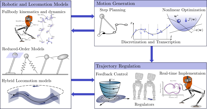
As we examine this brief historical outline of key developments in dynamic walking, it can be observed that with each new proposed methodology comes a greater understanding of how to model, plan, and execute increasingly complex behaviors on these robotic systems. Due to the inherently difficult nature of dynamic walking, successes in the field have typically been achieved by considering all aspects of the problem, often with explicit consideration of the interplay between modeling and feedback control (see Fig. 1). Specifically, the robotic and locomotive models which are used ultimately inform the planning problem and therefore the resulting behavior. Controllers which can actuate and coordinate the limbs must then be developed which, ideally, provide tracking, convergence and stability guarantees. In this review, we therefore examine how this interplay between modeling, motion planning, and trajectory regulation has shaped the dynamic walking on bipedal robots to date.
The remainder of this paper is structured as follows. In Section 2 we present reduced-order models that have provided canonical examples of dynamic locomotion, and in Section 4 we introduce extensions to hybrid system models for dynamic walking. Section 7 discusses how these models have been used to generate stable walking motions through various motion planning approaches and corresponding optimization problems. Finally, Section 8 provides several existing methods for controlling the robot as informed by the methods introduced in the earlier sections, with a view toward hardware realization. This interconnection can be seen in Figure 1, where each subsequent section is informed by the prior.
2 DYNAMIC MODELS OF BIPEDAL LOCOMOTION
In this section, we provide background on the modeling of dynamic bipedal robots and contextualize several of the most popular approaches for encoding or approximating locomotion via reduced order models. A unifying theme among the broad spectrum of models used for legged locomotion, both in this section and the next, is that the system must undergo intermittent contact with the surrounding environment in order to move. This fact is inexplicably tied to legged locomotion. How the overall walking system is ultimately modeled plays a critical role in the planning and control approaches that realize locomotion.
2.1 Bipedal Robots: Floating Base Systems with Contacts
Bipedal robotic platforms are conveniently modeled using a tree-like structure with an ordered collection of rigid linkages. This structure lends itself well to generalization, and thus tools to facilitate the generation of symbolic [22] or algebraic [23] expressions for the kinematics and dynamics of the robot are commonly used. The robot itself must ambulate through a sequence of contact conditions with the environment. Because interactions with the environment are always changing, a convenient method for modeling the system is to construct a representation of the robot in a general position, and then enforcing ground contacts through forces arising from the associated holonomic constraints that are imposed at the feet. This is often referred to as the floating-base model of the robot.
2.1.1 The Configuration Space
In order to represent the floating-base, let be a fixed inertial frame attached to the world and let be a body reference frame rigidly attached to the pelvis of the robot with the origin located at the center of the hip. Then the Cartesian position and orientation compose the floating base coordinates of frame with respect to . The remaining coordinates which dictate the shape of the actual robot, , are the local coordinates representing rotational joint angles and prismatic joint displacements. An image of this floating base coordinate system definition for a Cassie bipedal robot is given in Figure 2(a). The combined set of coordinates is with the states .
2.1.2 Continuous Dynamics
Traditional methods for modeling the dynamics of floating-base systems typically result in the separation of the equations of motion into multiple parts [24]; one arising from the multibody continuous dynamics, and the other imposed via constraints on contacts with the environment. If we continue with the assumption that the robot structure is a rigid collection of linkages then we can consider the continuous dynamics of a bipedal robot in the Lagrangian form (see [25]):
| (1) |
where is the inertia matrix, contains the Coriolis and gravity terms, is the actuation matrix, is the control input, and the Jacobian of the holonomic constraints applied to the robot is with the corresponding wrenches . These dynamics can be expressed in a state-space representation as:
| (2) |
2.1.3 Contact Forces
The fact that the robotic model is derived using a floating-base representation means that as we manipulate the robot, the resulting ground force interaction through the Lagrangian dynamics in Equation 1 is critical. The most popular method for modeling ground interaction is to assume rigid contacts with nonpenetration, the resulting forces are then considered to be unilateral [24], meaning that they can push and not pull on the ground. The resulting normal force cannot be negative, , and this implies that when this condition crosses zero that the contact will leave the ground. A point of the robot in static contact with the ground will satisfy a closure equation of the form:
| (3) |
where is the Cartesian position of the contact point and is a rotation between contacting bodies [26]. Differentiating twice yields acceleration constraints on the robot:
| (4) |
leading to a system of equations, with Equations 1 and 4 coupling the accelerations to the inputs and resulting constraint forces. The geometry of robotic feet is often given as either a flat foot or a single point of contact, shown in Figure 2(b). Assuming three non-collinear points of contact, the foot can be modeled as a flat plane. The position and orientation of the plane with respect to the ground will then create a degree-of-freedom (DOF) closure constraint in Equation 3 (). Alternatively, many underactuated robots have point-feet. If the assumption is made that the foot will not yaw while in contact, then this will form a DOF constraint on the Cartesian positions and rotation about the -axis ().
Finally, when designing motions for the robot it is important to also model the real-world limitations to the allowed tangential force before it will break a nonslip condition. The most popular approach is to employ a classical Amontons-Coulomb model of (dry) friction [26]. For a friction coefficient , the space of valid reaction forces is characterized by the friction cone:
| (5) |
2.2 Linear Inverted Pendulum and the Zero Moment Point
In this section, we describe the basic aspects of the Zero Moment Point (ZMP) and how it has been used in linear inverted pendulum models (LIPM) of locomotion. The concept of the ZMP is identical to the center of pressure (COP), and was originally introduced through a series of observations on the stability of anthropomorphic walkers by Vukobrativic̀ in the early ’s [27, 3]. The primary interpretation of the ZMP is: the point on the ground at which the reaction forces between the robot’s contacts and the ground produce no horizontal moment. Consider a robot standing in single-support, with a finite number of contact points () that constrain the foot to be flat. As shown in Figure 3(a), the resultant forces will consist of normal () and tangential components (). The ZMP is then computed as:
| (6) |
This led to perhaps the most commonly used dynamic stability margin [28, 29, 30, 31, 32], referred to as the ZMP criterion, which states that a movement is stable so long as the ZMP remains within the convex hull of the contact points (also known as the support polygon). This notion is conservative, and controlling these motions typically require the robot to remain fully actuated, with position controlled joints and load cells in the feet.
The ZMP criterion has been tied extensively to the linear inverted pendulum model (LIPM) in order to considerably simplify the trajectory design process, as the ZMP can be written explicitly in terms of the COM dynamics [33]. This has led to many researchers to consider a Newton-Euler representation of the centroidal dynamics, written as:
| (7) |
with the COM position, the angular momentum, gravitational acceleration, the contact forces, is each contact force position, , the linear and angular velocities on the -th linkage, , are the masses and inertia tensors, and the total mass of the robot. If we constrain the motion of a fully actuated inverted pendulum with a massless telescoping leg such that the COM moves along a horizontal (x,y) plane, then we obtain a linear expression for the robot dynamics. An example of the LIPM is visualized in Figure 3(b). The dynamics of the LIPM at a given height, , is:
| (8) |
where is the mass of the robot, is the acceleration of gravity, and , are the torques about the and axes of the attachment to the ground, i.e., the ankle. The ZMP location on the ground can also be directly written in terms of the LIPM dynamics as:
| (9) |
The LIPM can be viewed as a cart-table system [4], where the cart-table lies on a base with a geometry corresponding the the support polygon [34]. Designing walking with the ZMP can be essentially reduced to an inverse kinematics problem, where the primary planning is done on the ZMP trajectory. Figure 3(c) shows an example ZMP trajectory for several forward steps, wherein the trajectory for this walking is planned so that the ZMP always stays within the support polygon. ZMP walking has largely been applied to humanoids, such as the WABIAN robots [1], HRP series [7, 9], Johnnie [35], and HUBO [10].
2.3 Capturability and Nonlinear Inverted Pendulum Models
Rather than characterize the stability of walking based on the ZMP, Pratt [36] and Hof [37] independently introduced the idea of a Capture Point (CP), referred to as the “extrapolated center of mass” (XCOM) by Hof. The CP can be intuitively described as the point on the ground onto which the robot has to step to come to a complete rest. In canonical examples of the CP methods, the overall walking motions of the robot are planned and controlled based on the (instantaneous) capture point (ICP) dynamics. In this case, the COM of the robot is constrained to move at a constant height along a horizontal plane, and thus uses a LIP representation of the robotic system. It was shown in [38] that for the compound variable , that the unstable portion of the resulting system dynamics (along the horizontal direction) can be written in a constrained fashion as follows:
| (10) |
where is the horizontal location of the ICP. The main consideration of the locomotion process is then to ensure that feet are placed such that lies within the support polygon. Satisfying this condition means that the COM will converge to the CP and come to a rest. Despite this intuitive representation of stability, the LIPM walking simplifications come with a steep cost due to the stringent requirements on the motion and actuation of the robot. Yet it is precisely these characteristics which make the model most suitable for performing complex multi-objective tasks which include manipulation during intermittent conservative motions. The maturity and reliability of the LIPM made it prevalent in the walking controllers used at the DARPA Robotics Challenge [39, 40, 41].
In an attempt to overcome issues associated with the strict assumptions of the LIPM, researchers have introduced more complex pendulum models (illustrated in Figure 4(a)). The largest constraint on LIPM walking is the constant center of mass height assumption, leading to the development of a nonlinear inverted pendulum with variable mass height [42]. To account for the inertia of a swinging leg, the addition of a mass at the swing foot was proposed and termed the Gravity Compensated LIPM [43]. One of the most commonly used models in the literature to address nontrivial angular momenta from the limbs of large robots moving dynamically is to add a flywheel to the hip, which can be used to represent the inertia of the robot body as it moves [44]. A flywheel model of the robot has gained recognition as a convenient representation of the robotic system particularly for CP control [36, 45]. Various pendulum models have been widely used in analysis of push recovery and balance [46, 47, 48, 49]. The CP approach has also been used to demonstrate walking successfully on hardware [50, 38], and was famously used on Honda’s ASIMO [51, 52].
2.4 Spring Loaded Inverted Pendulum
Classic work by Raibert on hopping and running robots in the s demonstrated the efficacy of using compliant models in locomotion through the development of a planar hopper which could bound at a speed of m/s [11] and a 3D hopper which could achieve running without a planarizing boom [12]. These early successes drove researchers to investigate a Spring Loaded Inverted Pendulum (SLIP) representation of bipedal robots, shown in Figure 5(a). The SLIP model provides a low-dimensional representation of locomotion which draws inspiration from biological studies on animal locomotion [53, 54]. The SLIP is particularly attractive due to its inherent efficiency and robustness to ground height variations.
In order to use this model to synthesize controllers for actual robots, the control objectives are typically decomposed into three components: (1) achieving a particular footstrike location to regulate forward speed, (2) injecting energy either through passive compliance or motors to regulate the vertical height of the CoM, and (3) regulating the posture of the robot. One then designs the walking and running motions with SLIP models and compensates for model mismatch or disturbances with well tuned foot placement style controllers [55, 56, 57, 58, 59] (see Section 8.2). To this end, the dynamics of the SLIP are derived by assuming that the mass of the robot is concentrated at the hip with virtual springy legs:
| (11) | ||||
where is the stance leg length, is the stance leg angle, and is the force arising from the spring compression. One of the signature characteristics of this model is the “double hump” profile of the reaction forces, shown in Figure 5(b), described by the force interactions observed in biological walkers [54]. A key contribution introduced by the SLIP community is the handling of underactuated behaviors, with many of the corresponding robots having point-feet and flight phases of motion. Finding a stable gait thereon does not rely on the quasi-static assumptions used for the fully actuated pendulum walkers of the preceding sections—instead focusing on stable cyclic locomotion. Dynamic stability is defined based on a constraint on the periodicity of the walking (detailed in the sidebar “Periodic Notions of Stability”). To achieve forward walking, the initial states of the robot and the angle of attack for the swing leg are chosen to yield a periodic gait; see Figure 5(c). It is important to note that since the legs are massless, impacts are not considered, and the resulting orbit will be closed with no instantaneous jumps in the velocity.
[t]
3 Periodic Notions of Stability
One can view steady state walking as a periodic motion which is not instantaneously stable, but is stable from footstrike to footstrike [60]—in other words, walking is “controlled falling.” Concretely, a solution to a dynamical system is periodic if there exists a finite such that for all and a set is a periodic orbit if for some periodic solution . In a seminal paper on passive dynamic walking [14], McGeer popularized the method of Poincarè to determine the existence and stability of periodic orbits [61] for walking. In this approach, one step is considered to be a mapping from the walkers state at a definite point within the motion of a stride (typically defined at footstrike) to the walker’s configuration at the same point in the next step, . Let define the Poincarè section, for which we have a Poincarè map that maps one step to the next as . The periodic orbit yields a fixed point with , and stability of the orbit is equivalent to the stability of the Poincarè map which can be checked numerically [62, 63].
The SLIP representation of walking has been primarily used for legged robots which have springs or series-elastic actuators (SEAs). Some of the earliest inclusions of compliant hardware on bipedal robots was with spring flamingo and spring turkey [64]. Later, the COMAN robot included passive compliance to reduce energy consumption during walking [65], and the Valkyrie robot from NASA was the first full-scale humanoid robot to heavily use SEAs [66]. Using inspiration from the SLIP morphology, Hurst designed the planar humanoid robot MABEL [67] and the 3D bipedal robot ATRIAS [68, 69] to include series elastic actuation and thus return energy through impacts and shield the motors from impact forces at footstrike. One of the latest robots in this series, the Cassie biped (shown in Figure 2(a)) also mechanically approximates SLIP design principles [70]. Several running robots have specifically considered SLIP model principles in their mechanical design such as the ARL Monopod II [71], the CMU Bowleg Hopper [72], and the Keneken hopper [73].
4 HYBRID SYSTEM MODELS OF BIPEDAL LOCOMOTION
In the drive to obtain efficient legged locomotion and understand the stability thereof, researchers have adopted more dynamic paradigms for robotic locomotion which consider nontrivial impacts and periodic notions of stability. To formalize this perspective, it is necessary to consider hybrid system models of walking, which include both continuous (leg swing) and discrete (footstrike) dynamics. This section discusses to key paradigms that leverage this framework: passive dynamic walking, which exploits the natural hybrid dynamics of the system to obtain efficient walking, and hybrid zero dynamics which uses actuation to achieve model reduction and thereby synthesize stable walking gaits.
4.1 Passive Dynamic Walking
[b]
5 Hybrid Dynamical Systems
A hybrid dynamical system, used to model a walking robot [74], is defined as the tuple:
- •
is a directed cycle specific to the desired walking behavior, with the set of vertices and the set of edges, with , in the cycle.
- •
is the set of domains of admissibility. Each domain can be interpreted as the set of physically realistic states of the robot.
- •
is the set of guards, with which form the transition points from one domain, to the next in the cycle: .
- •
is the set of reset maps, from one domain to the next. The reset map gives the post impact state of the robot: .
- •
is a set of dynamical systems where for coordinates , i.e., of the form given in Equation 2 with .
Some of the first work to study hybrid systems for the purposes of synthesizing walking were within the field of passive dynamic walking. Tad McGeer [14, 75] introduced several passive walking robots that could ambulate down small declines when started from a reasonable initial condition. While these early bipeds were completely passive and relied on gravity, several bipeds were built to demonstrate that simple actuators could substitute for gravitational power and compensate for disturbances. Small electric actuators were used for the Cornell walkers [76, 77, 78] and the MIT learning biped [79, 80], while the Delft biped instead used a pneumatic actuator at the hip [81, 82]. Controlled symmetries [83] and geometric reduction [84] has been used to extend these ideas to actuated robots and 3D walking. Actuated environments have also been used to excite walking on passive robots [85]. Because of the care taken in mechanical design, these robots could all operate without sophisticated real-time calculations—though at the cost of diminished control authority.
The governing equations of motion for passive dynamic robots are nonlinear, and correspond to the continuous dynamics derived in Equation 1 rather than using an approximate (or reduced order) model. They are also hybrid, meaning they consist of both continuous and discrete nonlinear dynamics. A definition of the hybrid representation of the dynamics of walking is summarized in the sidebar “Hybrid Dynamical Systems”, where the key element that determines the behavior is a directed cycle of continuous domains.
5.0.1 Discrete Dynamics: Impacts and Poincarè Maps
An inherent feature of dynamic walking is that the robot is moving quickly through the environment. Thus the resulting motions cannot be slow enough for the feet to approach the ground with negligible velocity; impacts with the ground, therefore, become an important consideration in dynamic walking. Formally accounting for impacts underlies the basis for hybrid dynamical locomotion models [16, 26, 74]. Impacts during walking occur when the non-stance foot strikes the ground. Concretely, consider the vertical distance (height) of a contact point (foot) above the ground: . Impacts occur when the system reaches the switching surface of the guard:
| (12) |
where this surface is also a Poincarè section that will be used to construct the Poincarè map. At each transition, the new initial condition is determined through the reset map:
| (13) |
where is a relabeling matrix [16, 86], which “flips” the stance and non-stance legs. Here describes the change in velocity that occurs at impact, and is typically calculated using the assumption of a perfectly plastic impact [87, 88]. Note that determining and utilizing more complex impact models is an open problem. In real life, impacts are not truly instantaneous and do not always achieve stiction [89]. Situations with multiple impacts can arise [90] leading to Zeno behaviors [91, 92, 93], or slippage [94, 95].
A canonical example of passive dynamic walking is an unactuated compass biped walking down a slope of angle [96], shown in Figure 6(a). This robot consists of two kneeless legs each with a point-mass and a third mass at the hip. The directed cycle for the biped consists only of a single-support domain, with transition occurring at footstrike (shown in Figure 6(b)). The periodic nature of the stable walking behavior is best summarized by the phase portrait given in Figure 6(c), where there are discrete jumps occurring at impact. The stability of a cyclic gait is discussed in the sidebar “Periodic Notions of Stability”. Once a fixed point has been found, we can examine a first order expansion of the Poincarè map:
| (14) |
where the fixed point is exponentially stable if the magnitude of the eigenvalues of are less than one [61, 62, 63]. This is straightforward to check numerically: one can construct a numerical approximation of successive rows by applying small perturbations to each corresponding state and then forward simulate one step to obtain .
[b]
6 Hybrid Control Systems
Rather than describing a passive hybrid system as in the sidebar “Hybrid Dynamical Systems”, the incorporation of a feedback control allows for the realization of more advanced behaviors on complex actuated bipedal robots. We therefore define a hybrid control system [74, 97] to be a tuple:
6.1 Hybrid Zero Dynamics
The method of hybrid zero dynamics (HZD) leverages nonlinear feedback control design to induce stable locomotion on underactuated robots. Jessy Grizzle et al. [15, 98, 99] introduced the concept and developed a set of tools which are grounded in nonlinear control theory to deal formally with the nonlinear and hybrid nature of dynamic walking (cf. the textbook [16]). The basis of the HZD approach is the restriction of the full-order dynamics of the robot to a lower-dimensional attractive and invariant subset of its state space, the zero dynamics surface, via outputs that characterize this surface. If these outputs are driven to zero, then the closed-loop dynamics of the robot is described by a lower-dimensional dynamical system that can be “shaped”to obtain stability. As was the case for uncontrolled hybrid models generalizing hybrid dynamical systems, a hybrid control system (see sidebar) describes an actuated walking robot, leading to the notion of hybrid zero dynamics. The primary consideration which governs the overall locomotion problem is the specification of a directed cycle for the underlying hybrid (control) system. Because HZD incorporates feedback control, significantly more complex motions are possible. Examples of directed cycles for dynamic walking behaviors are given in Figure 7, illustrating how domain specification is governed largely by the evolution of the contacts through the course of a step. The controlled compass walker [96] is presented in Figure 9 to provide a comparison to the passive dynamic walking. In this example it can be seen that torques applied at the hip are used to control the motion, while the robot walks with a stable limit cycle on flat ground.
6.1.1 Virtual Constraints and Stabilization
Dynamic walking which leverages the fullbody dynamics must necessarily include specifications on how the robot should coordinate its limbs in a holistic fashion. To this end, and analogous to holonomic constraints, virtual constraints are defined as a set of functions that regulate the motion of the robot to achieve a desired behavior [16]. The term “virtual” comes from the fact that these constraints are enforced through feedback controllers instead of through physical constraints. Let be functions of the generalized coordinates that are to be controlled, i.e., encoding the “actual” behavior of the robot and be the “desired” behavior where is a matrix of real coefficients that parameterize this behavior. A Bézier polynomial is the most typical choice of representation for the desired outputs [16] for computational reasons, though it has been shown that humans appear to follow spring-mass-damper type behavior [86]. Given actual and desired outputs, a virtual constraint is their difference:
| (15) |
with a parameterization of time that is strictly increasing along periodic motions. Driving results in convergence of the actual outputs to the desired.
To synthesize controllers, note that differentiating along solutions to the control system in Equation 2 yields the Lie derivatives:
| (16) |
wherein has vector relative degree 2 [100] if the matrix is invertible. From this, one obtains the following feedback linearizing controller:
| (17) |
where is the auxiliary feedback component of the controller that can be chosen to stabilize the system. In particular, one common choice is , with , feedback gains chosen so that the linear dynamics are stable, and a parameter used to amplify convergence to the desired motion; rendering the output dynamics exponentially stable. Applying Equation 17 with results in the closed-loop system:
| (18) |
wherein for this system exponentially fast.
6.1.2 Hybrid Invariance
The feedback control law of Equation 17 can be synthesized for virtual constraints associated with each domain , , and control system: . This renders the zero dynamics manifold [101]:
| (19) |
forward invariant and attractive. Thus, the continuous dynamics in Equation 18 will evolve on given an initial condition in this surface. However, because the surface in Equation 19 has been designed without taking into account the hybrid transition maps of Equation 13, the resulting walking cycle may not be invariant to impact. To enforce impact invariance, the desired outputs can be shaped through the parameters in such that the walking satisfies the hybrid zero dynamics (HZD) condition:
| (20) |
imposed as a constraint on the states through impact (Equation 13).
The overarching goal of these constructions is to provide a framework for the synthesis of dynamic walking gaits. In this context, for simplicity (and without loss of generality) assume a single domain wherein we will drop the subscript “.” For the full-order dynamics, let be the (unique) solution at time with initial condition . For a point we say that is hybrid periodic if there exists a such that . Further, the stability of the resulting hybrid periodic orbit, , can be found by analyzing the stability of the Poincaré map, wherein is a fixed point, as previously presented in Equation 14. The main idea behind the HZD framework is, due to the hybrid invariance of , if there exits a stable hybrid periodic orbit, , for the reduced order zero dynamics evolving on , i.e., the restriction of to , then is a stable hybrid periodic orbit for the full order dynamics in Equation 19 [16]. A visualization of the components of HZD walking design is given in Figure 8.
In the case of robots which have feet, as is the case for many humanoid robots, one can extend the concept of HZD to modulate the forward velocity of the robot [102]. In particular, one can generalize HZD through a velocity modulating output: , with the desired forward velocity. One can augment the original virtual constraints with this new (relative degree) output. The partial hybrid zero dynamics surface is, again, given as in Equation 19 where the term “partial” is used since this surface does not require the output to be zero. Partial hybrid zero dynamics (PHZD) is the condition: . In the case of full actuation the existence of hybrid periodic orbit, in , is guaranteed implying the existence of a hybrid periodic orbit for the full order dynamics. Thus, PHZD implies the existence of a stable gait for fully actuated robots.

6.1.3 Application of HZD
In the context of robotic implementations, HZD has proven successful in realizing a wide variety of dynamic behaviors. Many of the early uses of the method were on point-footed robots which were restricted to the sagittal plane. The first robot used to study HZD was the Rabbit biped [103], followed later by MABEL [104] and AMBER [105]. The ability of (P)HZD to handle multidomain behaviors led to its use on more complex planar bipedal robots such as ATRIAS [106, 107], AMBER [108] and AMBER M [109]. New challenges appeared while extending the method of HZD from planarized robots to 3D robots, which exhibit additional degrees of underactuation. Control of fully actuated humanoids was demonstrated on a small-scale example with a NAO robot [110] via PHZD, while point-footed 3D walking with HZD was first shown at the University of Michigan with the MARLO biped [111]. At the DARPA Robotics Challenge, the humanoid DURUS (shown in Figure 10(a)) was featured in an efficiency walk-off [20] where it demonstrated the first sustained humanoid HZD walking—over five hours continuously. DURUS went on to exhibit the most efficient walking on a humanoid to date, while performing human-like multicontact behaviors and managing significant underactuation [21]. The method has been extended to powered prosthetic walking [112, 113, 114] and to exoskeletons which can walk for patients with paraplegia [115, 116]. The use of springs in locomotion has also proven useful in the development of dynamic walking behaviors, though it presents additional challenges both mathematically and in practice. The notion of compliant hybrid zero dynamics was introduced in the late ’s [117], and was later expanded upon to obtain compliant robotic running [18]. One of the latest robots to successfully demonstrate stable HZD walking is the Cassie biped, shown in Figure 2(a), where it can be seen that the robot exhibits underactuated feet and passive springs in the legs. Dynamic walking on Cassie has been successfully realized on hardware both by planning under the assumption of sufficient rigidity in the legs to ignore compliant elements [118], and for walking which considers the passive compliance in the zero dynamics [119].

[Experimental Highlight: Hybrid Zero Dynamics] We highlight the application of HZD by considering its experimental realization on hardware. Leveraging PHZD on DURUS and HZD on Cassie, the result is stable periodic orbits—both in simulation and experimentally—as illustrated in Figure 7. The evolution of the dynamic walking motion is tied to the morphology of the robot, with the humanoid DURUS exhibiting human-like heel-toe walking [102, 21] and the Cassie biped leveraging a domain structure and outputs which correspond to the SLIP inspired mechanical design [119]. In these specific examples, the virtual constraints chosen are shown in Figure 10. This demonstrates one of the benefits of HZD: the ability to chose virtual constraints to formally encoded reduced order models for complex robots and correspondingly “shape” the zero dynamics surface to render it stable.
7 MOTION GENERATION FOR DYNAMIC BIPEDAL LOCOMOTION
Throughout the previous section, we outlined how the locomotion problem is fundamentally different than traditional approaches to modeling fixed-base robots. It is because of this inherent complexity that virtually all approaches to realize dynamic walking must transcribe the locomotion problem into a motion planner which can handle the various constraints naturally imposed on the problem. While several of the more classical walking paradigms offer simple solutions to conservative walking, there has been a push over the last two decades towards leveraging optimization to obtain increasingly dynamic maneuvers.
7.1 Step Planning with Linear and Reduced-Order Models
Often for the simplest models of walking, such as traditional ZMP and LIPM versions of CP, the linear dynamics of the restricted system yield straightforward approaches to planning the motion of the COM. The walking characterized by these linear models often implicitly satisfy quasi-static stability assumptions, ultimately allowing a control designer to decouple the high-level step planner and low-level balance controllers [120]. In this vein, Kajita [34] introduced the jerk of the COM as an input controlled by a discrete LQR controller with preview action [121] to plan ZMP trajectories for predefined footsteps. However, predefining the motions of the ZMP or footholds is not always necessary or desirable.
If planners for these simple models could instead be performed online, then the robot may be able to mitigate issues related to reactivity. Weiber [122] proposed using linear trajectory-free model predictive control (MPC) as a method for explicitly handling the constraints imposed by the ZMP approach of Section 2.2 while continuously re-evaluating the walking path. Stephens [123] presented the use of MPC for push recovery and stepping on the SARCOS humanoid, which could be extended to obtain walking behaviors. The example shown in Figure 3(c) visualizes the result of this MPC approach applied to LIPM robotic walking. It has also been shown how optimization and model predictive control can extend the notions of capture point to viable regions on which the biped can step [124], or how push recovery can be planned over a horizon of multiple steps [38]. Despite the ability of these planners to adapt online, they cannot handle the discrete dynamics associated with footstrike, and demand near-zero impact forces [125]. This rules out the nontrivial impacts which are naturally associated with dynamic walking. It also difficult to provide a priori guarantees on whether any given reduced-order plan is feasible to execute on the full-order dynamics. Such methods typically use inverse kinematics [126], or inverse dynamics [127] sometimes in an operational-space formulation [128] to compute the full-order control inputs at each instant. Solving such near-term inverse problems does not imply that future inverse problems in the trajectory will be feasible, which requires additional planning [129, 130].
7.2 Nonlinear Optimization for Gait Generation
As a result of the rapid developments within the trajectory optimization community, researchers began to move towards utilizing nonlinear dynamic gait optimizations rather than relying on the constraints imposed by linear modeling assumptions. The use of nonlinear optimization, i.e., numerical approaches, to generate stable walking behaviors on bipeds not a new concept [131, 132], though computational limitations were a considerable hindrance towards generating motions on 3D robots. Computation power finally increased sufficiently throughout the mid ’s to begin handling 3D dynamic walking behaviors [133].
7.2.1 Open-Loop Optimization
The simplest application of nonlinear optimization to walking can be found in Section 4.1, wherein passive dynamic walking relies on the generation of fixed points associated with periodic orbits of a hybrid dynamical system. This naturally lends itself to numerical approaches for the optimization of open-loop stable periodic motions [134], since passive dynamic walkers do not have any actuators to consider. The use of open-loop optimization to generate feasible motions for actuated robots are a natural extension of approaches used throughout the field of trajectory optimization, where the planning problem is seen as “decoupled” from the feedback control applied to the actual robot [135] and “approximately optimal” solutions are often sufficient. Further, in recent years, the application of advanced trajectory optimization methods such as direct collocation have allowed the optimization of the full body dynamics of Equation 1 to be more computationally tractable, sparking a growing interest in considering the fullbody dynamics of robot in the planning problem. For instance, in order to control the open-loop trajectory that results from the direct collocation optimization, a classical linear quadratic regulator (LQR) based feedback controller can be constructed to stabilize the resulting trajectory obtained for the constrained dynamical system [136]. In this type of approach, the walking problem can be viewed as generating sequences of footholds for the nonlinear centroidal dynamics given in Equation 7 [137, 40] or with respect to the full Lagrangian system given in Equation 1 [138]. Complementary Lagrangian systems [139] formed the basis of the approach in [138], which allowed the optimizer to find walking behaviors without a priori enumeration of the type and order of contact events. Open-loop trajectory optimization has also been used to satisfy ZMP conditions in a nonlinear fashion [140], which considerably improved the dynamical nature of the conservative walking presented in Section 2.2.
7.2.2 Closed-Loop Optimization
While the preceding nonlinear optimization approaches do consider the fullbody dynamics of the robot, it is not always desirable to apply feedback controllers to stabilize an approximately optimal open-loop plan. Rather, it is often beneficial to couple the gait generation and controller synthesis problems into a single framework: closed-loop optimization. This allows, among other things, for the generation of provably stable walking behaviors which simultaneously satisfy the constraints on the system from admissible configurations to torque bounds. This idea forms the basis of designing walking gaits with the HZD method introduced in Section 6.1, where feedback control is used to generate provable stable periodic orbits. A visual summary of this section is given in Figure 12. By applying these closed-loop feedback strategies in the optimization problem, ambiguous contact sequences are no longer possible [141] and must be prescribed according to the directed cycle which governs the underlying hybrid system (see Figure 7). Doing so allows for one to enforce physical feasibility constraints, e.g., unilateral contact, in conjunction with the synthesis of controllers that guarantee stability.
In the context of HZD methods, with the formal constructions of the zero dynamics (Equation 19) and hybrid invariance (Equation 20) defined, the problem of finding stable dynamic walking can be transcribed to a nonlinear programming (NLP) problem of finding a fixed point and set of parameters parameterizing the virtual constraints of Equation 15. The optimization problem is performed over one step cycle, e.g., footstrike to footstrike, with a constraint imposed such that when the discrete impact (Equation 13) is applied to the terminal state so that it satisfies the hybrid invariance condition of Equation 20. It is also critical that the motions respect the limitations of the physical system such as the friction cone (Equation 5), actuator limits, and joint limits. These constraints can be directly placed into a NLP problem that can be solved by a standard optimization solver:
| (21) | ||||
| Closed loop dynamics: Equation 18 | ||||
| HZD condition: Equation 20 | ||||
| Physical feasibility (e.g. Equation 5) |
where , with being the total number of optimization variables and here we made the dependence on the parameters, , that dictate the closed loop dynamics explicit. With the goal of achieving dynamic and efficient walking, a common objective is to minimize the mechanical cost of transport (M-COT) of the walking gait through the cost [20, 141]. In classical HZD implementations, the candidate solutions were found via single shooting formulations [15, 102], where the decision variables are the fixed point states and the output coefficients . Because single shooting optimizations are notoriously sensitive to poor initial conditions, multiple shooting was also explored [142], with the eventual development of direct collocation formulations [143] which would become the most successful to date. The FROST optimization package [22] was developed based on these successes as an open-source package to transcribe HZD locomotion into a direct collocation problem. While HZD optimization problem determines one stable walking orbit, it has been shown that one can expand the range of motions a robot can perform through systematic optimization to build libraries of walking parameters [144]. Reinforcement learning has also been used to handle robust transitions for different speeds or unknown terrain height disturbances [145].
[Experimental Highlight: Closed-Loop Optimization] The use of closed-loop optimization for HZD behaviors yields a set of outputs which coordinate the motion of the robot. This is shown as the output of the process in Figure 12, where the nonlinear optimization problem has provided outputs which yield orbital stability for compliant HZD [119]. The outputs which are shown directly correspond to the SLIP-like morphology of the robot, emphasized in Figure 10. Reference trajectories can be shaped by the cost to yield desirable gait characteristics, such as efficiency on DURUS, or for minimizing torque and extraneous movement on Cassie to obtain behaviors which leverage the compliance for propulsion.
8 FEEDBACK CONTROL AND MOTION REGULATION
While the dynamic walking paradigms introduced throughout the previous sections generate stable walking motions in simulation, their actual implementation requires the deployment of real-time feedback controllers capable of achieving the desired motions. As described in Section 2.1, dynamic walking robots involve a high level of complexity in the form of nonlinearities and tightly coupled equations of motion which must be considered. In the case when locomotion has been planned using a simplified model (Section 2.1, the spatial geometry of the robot must be translated into joint angles which can be controlled. Even with a full-order hybrid model (Section 4) and closed-loop optimization (Section 7), controllers must be synthesized in order to track these desired motions in practice. This section describes feedback controllers and motion regulators that allow for the translation of dynamic walking in simulation to be realized on real-world hardware platforms.
8.1 Controllers for Tracking Designed Motions
The simplest control scheme for determining motor torques is Proportional-Derivative (PD) control [146]. The strongest argument for using this approach is the sheer simplicity in its implementation and the intuitive physical meaning with respect to tuning. Consider desired positions and velocities, and (and possibly functions of time), either obtained from inverse kinematics for reduced order walking models or the output of a optimization problem. A feedback controller can be applied at the joint level:
| (22) |
generating desired torques (or currents) that are tracked at the motor controller level at a fast loop rate. in the case of underactuated robots and/or virtual constraints (see Section 6.1.1), one can consider outputs of the form:
where the time-based variant is often considered in practice, especially in the case of 3D walking and running, due to imperfect sensing of wherein it is replaced by the more robust signal [19, 147]. Let represent the joints with actuators, then the PD controller can be applied in the Cartesian (or output) space:
| (23) |
where is the Jacobian of the Cartesian task or output with respect to the actuated joints, and are the PD gain matrices. This style of feedback control has been used to enforce the behaviors of every locomotion paradigm detailed in Section 2 and Section 4 at some point in time.
For underactuated dynamic walkers whose motions have been planned with virtual constraints, simply tracking the outputs with a well tuned PD controller is sometimes sufficient to achieve walking on hardware [148, 104, 144, 21, 119], and even running [19]. This is because the trajectories (or outputs) implicitly encode the dynamic behavior and stability constraints, even if it requires different torques on the actual robot to achieve these behaviors. In addition, because dynamic behaviors are often rendered stable through this behavioral encoding while satisfying appropriate physical constraints, almost all passive dynamic and HZD walkers to date have opted not to include load cells in the feet – as feedback control of these quantities is not necessary for stability. An example of PD controllers applied in experiment to two 3D bipedal robots is given in Figure 11, where it can be seen that although the motions do not track the designed motions perfectly they do form a closed orbit—implying stable walking.
In the context of reduced order models, plans for ZMP and CP have typically considered a point-mass representation of the robot under which whole-body momentum and force regulation becomes an important concern when developing feedback controllers for implementation. This has led to a variety of approaches which concurrently regulate the COM movement via some PD feedback element in combination with control of the whole-body momentum [149, 150, 151, 152] and tracking of desired force interactions [153, 154].
When the dynamics of the system are well known, it is often beneficial to leverage them in the feedback control design. One of the classical methods which was used for exploring this in the context of bipedal robots is computed-torque control, which considers an inner nonlinear compensation loop, and the design of an auxiliary control feedback [155, 43]:
| (24) |
where is the nominal system acceleration. Note that this is mathematically equivalent to feedback linearization, as given in Equation (17) (see [156]). Although both the standard PD controller and computed-torque approach can overcome minor disturbances, they are often not sufficient to formally ensure the stability or yield the performance that dynamic walking requires. This motivates the use of a controller which can provide good tracking performance while leveraging the robotic model. The remainder of this section will explore several of the approaches which have been successful in the feedback control of bipedal robots, and how these can be extended to provide formal stability guarantees.
[Experimental Highlight: Trajectory Tracking] The trajectories found in Section 7.2 for HZD are well suited to feedback controllers for output tracking problems. To demonstrate the simplest and yet effective implementations of PD controllers which have been successful in realizing dynamic walking, we show experimental results on hardware for DURUS and Cassie in Figure 13. This shows that for controllers in the joint space (Equation 22) and output space (Equation 23) dynamic walking is can be achieved by simply tracking the designed motion.
8.1.1 Inverse Dynamics
While PD control is sufficient for many applications, it fails to explicitly consider the model of the robot and the constraints under which it operates. Inverse dynamics is a widely used method to approach model-based controller design for achieving a variety of motions and force interactions, typically in the form of task-space objectives. Given a target behavior, the dynamics of the robotic system are inverted to obtain the desired torques. In most formulations, the system dynamics are mapped onto a support-consistent manifold using methods such as the dynamically consistent support null-space [157], linear projection [158], and orthogonal projection [159]. When prescribing behaviors in terms of purely task space objectives, this is commonly referred to as task- or operational-space control (OSC) [128]. In recent work, variations of these approaches have been shown to allow for high-level tasks to be encoded with intuitive constraints and costs in optimization based controllers, some examples being [160, 40, 161, 152, 162].
A benefit of inverse dynamics approaches to feedback control on robotic systems is that low gain feedback control can be used, while feedforward terms which respect the constrained rigid body dynamics of the physical system are used to produce the majority of the control action. If the walking is not significantly disturbed from the planned motion found in Section 7.2 then a linear null-space projection operator can be used to eliminate the contact forces from the floating-base dynamics in Equation 1 [158], using QR decomposition [159] to obtain an orthogonal projection into the null-space of .
The inverse dynamics problem can also be posed using a quadratic program (QP) to exploit the fact that the instantaneous dynamics and contact constraints can be expressed linearly with respect to a certain choice of decision variables. Specifically, let us consider the set of optimization variables , which are linear with respect to Equation 1 and Equation 4,
| (25) |
and a positional objective in the task space of the robot written as , where and is a PD control law which can be tuned to achieve convergence. An additional benefit to using an optimization-based approach is the ability to include feasibility constraints such as the friction cone (Equation 5). However, this constraint is nonlinear, and cannot be implemented as a linear constraint. An alternative solution is to use a pyramidal friction cone approximation [26],
| (26) |
which is a more conservative model than the friction cone but is advantageous in that it is a linear inequality constraint. In it’s most basic case, we can combine these elements to pose this QP tracking problem as:
| (ID-QP) | ||||
| s.t. | Equation 25 | ((System Dynamics)) | ||
| ((Torque Limits)) | ||||
| Equation 26 | ((Friction Pyramid)) |
where is included as a regularization term with a small weight such that the problem is well posed. Although this kind of control satisfies the contact constraints of the system and yields an approximately optimal solution to tracking task-based objectives, it does not provide formal guarantees with respect to stability. In increasingly dynamic walking motions this becomes an important consideration, wherein impacts and footstrike can destabilize the system requiring more advanced nonlinear controllers.
8.1.2 Control Lyapunov Functions for Zeroing Outputs
The methods presented thus far demonstrate how feedback control can drive the dynamics of the robotic system to behave according to the planned motions found in Section 7. However, these designs often intrinsically ignore the natural dynamics of the system, which is a critical component in the realization of efficient and dynamic walking. Thus, for practical systems, additional considerations for selecting our control input are often required. Rapidly exponentially stabilizing control Lyapunov functions (RES-CLFs), were introduced as methods for achieving (rapidly) exponential stability for walking robots [17, 163]. A function, , is a RES-CLF if it satisfies:
| (27) | |||||
| (28) |
for , and a control gain that allows one to control the exponential convergence of the CLF, and is the basis for the term “rapid” in RES-CLF. Importantly, if the robotic system is feedback linearizable per Section 6.1 it automatically yields a Lyapunov function. In particular, defining , we obtain RES-CLF: where with and the solution to the continuous time algebraic Riccati equations (CARE) for the linear system obtained by feedback linearization in Equation 17.
The advantage to controller synthesis with CLFs is that they yield an entire class of controllers that provably stabilize periodic orbits for hybrid system models of walking robots, and can be realized in a pointwise optimal fashion via optimization based controllers. In particular, consider the set of control inputs:
| (29) |
which is a set of stabilizing controllers. To see this, note that for :
| (30) | ||||
Thus, this gives the set of control values that exponentially stabilize the outputs and we can control the convergence rate via . The selection of an appropriate choice for the “best” control value possible leads to the notion of optimization based control with CLFs.
The advantage of Equation 29 is that it gives a set of controllers that result in stable walking on bipedal robots. That is, for any the hybrid system model of the walking robot, per the HZD framework introduced in 6.1, has a stable periodic gait given a stable periodic orbit in the zero dynamics [17]. This suggests an optimization-based framework nonlinear controller synthesis, with specific application to dynamic locomotion. Specifically, the optimization formulation of CLFs allows for additional constraints and objectives to be applied as a QP with the form (as first introduced in [156]):
| (CLF-QP) | ||||
| ((CLF Convergence)) | ||||
| ((Torque Limits)) | ||||
| Equation 26 | ((Friction Pyramid)) |
where is a user specified positive-definite cost, is a relaxation to the convergence constraint which can be added if infeasibility of the solution is a concern, and is a large value that penalizes violations of the CLF constraint. If the relaxation term is included then the formal guarantees on convergence are no longer satisfied in lieu of achieving pointwise optimal control actions which satisfy the physical constraints of the robot. Ground reaction forces on the robot also appear in an affine fashion in the dynamics; thus one can also use the CLF-based QP framework in the context of force control [156].

The CLF-based controllers presented throughout this section have recently been explored of interest for application on hardware, because much like the optimization controllers of Section 8.1.1 they can be solved in real-time. Experimental results have been shown on MABEL [17, 164] and DURUS-2D [165], with recent results indicating how robust formulations can be used [166] and how alternative representations can make the problem more tractable for implementation on 3D robots [167]. Additionally, it was implemented at over kHz as an embedded level controller on series elastic actuators [168], indicating possible future uses on explicitly controlling compliant dynamic walking. The use of CLFs has also been used to automatically generate stable walking gaits through SLIP approximations [169], and also to enforce planned motions for reduced order models [170] along with realizing 3D bipedal jumping experimentally on Cassie [171].
[Experimental Highlight: Real-Time CLF QP Control] We highlight the application of CLF based QPs on hardware in real-time in the context of dynamic crouching maneuvers on Cassie, shown in Figure 14 [119]. Because the CLF-QP can be run at a sufficient control frequency (in this case at kHz), these experiments show how convergence properties combined with inclusion of the model can lead to desirable tracking performance on complex bipedal robots. These methods are directly extensible to tracking walking trajectories, where the constrained pointwise optimization can select torques which satisfy the contact constraints governed by the discrete structure of the hybrid system model (see Figure 7).
8.2 Stabilizing Walking with Trajectory Modification

The prior sections detailed how dynamic walking behaviors are formulated, synthesized and tracked; yet, these components alone are often not sufficient to realize sustained and robust robotic walking on hardware. The final step in achieving robustness involves the “artful implementation” of modifying the desired behavior to account for unknown and unmodified disturbances – both specific to the hardware, e.g., unmodified compliance, and in the external environment, e.g., rough terrain. Approaches such as MPC planners and analytical expressions for the CP, presented in Section 7.1, can be evaluated in real-time to adapt the motion of the robot to avoid falling or recover from large pushes [123]. In these cases the planning and the real-time compensation are inherently tied [172], though they still are re-planning over an approximate the model of the robot and can lead to constrained motions which are prohibitive to truly dynamic walking. On the other hand, while the nominal trajectories of offline plans which consider the full-body continuous and hybrid dynamics are generated with high fidelity models (such as the motions found via Section 7.2) it is evident in experimental trials that some additional feedback is crucial to stabilizing the robot for sustained periods of walking. These nominal trajectories are often superimposed with some form of regulator in order to overcome uncertainties due to model mismatch and tracking errors, typically in the form of adding trajectory level feedback (see Fig. 15). The development of these regulators is a largely heuristic task, but has often proven critical to stability on hardware. A variety of different regulators have proven useful, though implementation largely dependents on the robotic system and desired behavior.
When performing dynamic maneuvers it is inevitable that the actual linkages of humanoid robots, which have large masses and inertias, can subject rotational joints to backlash and unsensed compliance. For these problems, using an experimentally measured stiffness coefficient to augment commanded positions based on anticipated torque at the joint has shown to be an effective compensation strategy [21, 39]. The combination of uncertainty in the kinematics and dynamics of the robot can also lead to predictable issues with gait timing on periodic walking behaviors. For dynamic walking which has been planned with a monotonic phase variable dependent on the state of the robot, there can be a large amount of uncertainty with regards to the estimation of the floating-base coordinates and therefore the phase [19, 147]. In these cases it can be beneficial to employ a combination of time and state based progression of the variable [144].
Another type of regulation comes in form of small modifications to the shape of the robot (i.e. superimposed perturbations to virtual constraints) from stride-to-stride. How this can be conceptually interpreted within the HZD framework is shown in Figure 15, where control designers seek to shape a perturbed zero dynamics surface such that the hybrid system returns to an orbit which satisfies hybrid invariance. In early developments for control of HZD walking, the restricted Poincarè map was viewed as a discrete-time control system [174]. Through consideration of the linearized map at the fixed point (see Equation 14), a discrete LQR algorithm can then be used to acquire a feedback gain to modify the configuration of the next footstrike [107]. This can be straightforward to design for 2D robots, but extensions to 3D become more difficult. Perhaps the most common approach is to instead utilize foot placement routines inspired by Raibert [11]. This simple deadbeat step-to-step controller most often takes the form of a discrete PD controller to augment the footstrike locations in the sagittal and frontal planes during locomotion:
| (31) |
where the average velocity of the current step and previous step are computed directly from an estimate of the floating-base velocity, and the reference velocity is taken from the nominal trajectory. In addition, because outputs for HZD walking are typically parameterized by a Bézier polynomial, the update value can directly augment the last two parameters of the corresponding output polynomials [173]. This kind of smooth transition is demonstrated in Figure 16(b), where the position has been smoothly modified, but the velocity at impact will remain the same. This simple foot placement regulator has been successfully implemented on several dynamic walking robots [144, 175, 119]. Rather than considering hand-tuned regulation, the notion of nonholonomic virtual constraints was introduced [176], aiming to formalize a representation of virtual constraints which are insensitive to a predetermined and finite set of terrain variations and velocity perturbations. Implementation of this approach required intensive optimizations, as the walking was made to be stable amid a variety of perturbations in each step of the optimization. This type of output-level feedback has also been proven to be successful in a more directly hand-tuned fashion, such as in [20, 21], where the position-level feedback of the outputs was governed by a proportional gain with respect to the pitch and roll of the robot’s torso. The superimposed motion will then be zero if the walking is directly on the orbit, but will smoothly apply a superimposed positional command if necessary. One interpretation of this regulator feedback is simply that has been made a function of the floating base coordinates of the robot, with an example shown on the DURUS humanoid in Figure 16(a).

[Experimental Highlight: Dynamic Walking] The experimental highlights considered throughout this this paper culminates with efficient and agile locomotion on DURUS and Cassie, as shown in Figure 17. The multicontact walking on DURUS demonstrated efficiency as evidenced by an exceptionally low cost of transport [21], achieved by leveraging hybrid models, to closed loop optimization, to real-time feedback controllers and regulators. The compliant walking on Cassie [119] demonstrates agility, through a wide range of walking speeds up to m/s, along with the ability to walk on unplanned rough terrain outdoors.
9 CONCLUDING REMARKS
This review article outlined the general methodology for achieving dynamic walking on bipedal robots. As outlined in “Summary Points,” we begin by considering reduced order models that capture the essentials of locomotion – yet these models are not sufficient for handling the full complexity of walking robots. This led to full order models that include impacts as represented by hybrid systems, wherein we considered hybrid zero dynamics. To generate walking gaits with these models, and corresponding dynamically feasible trajectories, the role of optimization was discussed. Finally, connecting models with walking gaits, real-time controllers that enable hardware realization were discussed; ranging from simple control methods, to advanced QP based controllers, together with the modification of these nominal desired values due to uncertainty in the system and environment. This end-to-end process was illustrated throughout on the bipedal robots DURUS and Cassie, wherein the translation to hardware and corresponding experimental results were highlighted.
Looking forward, the process of realizing dynamic walking that is efficient and agile is ripe with opportunities. Some of these challenges are highlighted in “Future Issues.” In essence, these can be subdivided into two categories: theoretic and practical. The overarching goal, theoretically, is to formally and holistically extend the methodologies presented. The hope is to, as a result, develop a framework that is capable of realizing aperodic dynamic motions that are stable and safe which are planned in real-time and robust to uncertainties in the robot and environment. From a practical perspective, hardware is ever improving and becoming more accessible. This gives the ability to better test approaches for agile and efficient walking in real-world scenarios. The goal is to finally realize the promise of dynamic walking: imbuing legged robots with the locomotion capabilities that will enable them to do everything from traversing everyday environments to exploring the cosmos. {summary}[SUMMARY POINTS]
- 1.
Reduced order models. At the core of dynamic walking is the idea of reduced order models. These are either hierarchical—representing desired behavior on simple models, e.g., inverted pendula and compass gait bipeds—or formally determined—low-dimensional systems rendered invariant by controllers, e.g., HZD.
- 2.
Full order nonlinear dynamics. Bipedal robots are inherently nonlinear with hybrid dynamical behaviors. These full order dynamics must be accounted for, either through assumptions thereon that yield reduced order models, through nonlinear controllers, or via optimization algorithms.
- 3.
Optimization for gait generation. Reduced order models must be instantiated on the full order dynamics via optimization algorithms. This can leverage reduced order models, exploit the full order dynamics, or any combination thereof. Algorithms that allow for these optimization problems to be solved efficiently are essential in instantiating walking gaits on hardware platforms.
- 4.
Control laws for hardware realization. Control laws allow for the generated gaits to, ultimately, be realized on hardware. These can range from simple control laws to complex nonlinear real-time optimization-based controllers, and can be modulated via inspiration from reduced order models. These control algorithms are the final step in realizing dynamic walking on bipedal robots.
[FUTURE ISSUES]
- 1.
Generalized notions of stability and safety. The walking considered herein, and the notions of stability, was largely periodic in nature. To better represent a wide variety of behaviors, the idea of stability should be extended to include aperiodic walking motions [177, 178]. More generally, safety as represented by set invariance [179] could provide a powerful tool for more generally understanding locomotion.
- 2.
Real-time optimal gait planning. It was seen that nonlinear constraint optimization plays an essential role in generate dynamic walking behaviors that leverage the full-body dynamics. These methods have become very efficient, even allowing for online calculation in simple scenarios [180]. Further improving computational efficiency will enable real-time implementation yielding new paradigms for gait generation.
- 3.
Bridging the gap between theory and practice. As indicated by the methods discussed in Section 8, there is often an “artful implementation” step that translates model-based controllers to a form that can actually implemented on hardware. Ideally, methods can be developed that allow the exact transcription of model-based methods to hardware in a robust fashion and without heuristics.
- 4.
Robustness, adaptation and learning. Dynamic walking behaviors often work in isolated instances and predefined environments. Translating these ideas to the real-world will require robustness to uncertainty – both in the internal dynamics and external environment. Adaptive and learning-based controllers can help mitigate model uncertainty and unplanned interactions with the world, from uncertain contact conditions to walking on surfaces with complex interactions, e.g., sand.
- 5.
Real-world deployment of bipedal robots. The ultimate challenge is the ability to deploy bipedal robots in real-world scenarios. This ranges from everyday activities, to aiding humans, to venturing into dangerous environments. Examples include bipedal robotics in a healthcare setting, e.g., exoskeletons for restoring mobility [116], to humanoid robots capable of exploring Mars.
DISCLOSURE STATEMENT
The authors are not aware of any affiliations, memberships, funding, or financial holdings that might be perceived as affecting the objectivity of this review.
ACKNOWLEDGMENTS
The authors would like to thank the members of AMBER Lab whom have contributed to the understanding of robotic walking summarized in this paper. Of special note are Shishir Kolathaya, Wenlong Ma, Ayonga Heried, Eric Ambrose and Matthew Powell for their work on AMBER 1, 2 and 3M and DURUS, from developing the theory, to computational methods, to experimental realization. Outside of AMBER Lab, the authors would like to thank their many collaborators. Of particular note is Jessy Grizzle and the joint efforts on HZD and CLFs. This work was supported over the years by the National Science Foundation, including awards: CPS-1239055, CNS-0953823, NRI-1526519, CNS-1136104, CPS-1544857. Other support includes projects from NASA, DARPA, SRI, and Disney.
References
- [1] Lim HO, Takanishi A. 2007. Biped walking robots created at Waseda University: WL and WABIAN family. Philosophical Transactions of the Royal Society A: Mathematical, Physical and Engineering Sciences 365:49–64
- [2] Vukobratovic M, Hristic D, Stojiljkovic Z. 1974. Development of active anthropomorphic exoskeletons. Medical and biological engineering 12:66–80
- [3] Vukobratović M, Stepanenko J. 1972. On the stability of anthropomorphic systems. Mathematical biosciences 15:1–37
- [4] Vukobratović M, Borovac B. 2004. Zero-moment point—thirty five years of its life. International journal of humanoid robotics 1:157–173
- [5] Collins S, Ruina A, Tedrake R, Wisse M. 2005. Efficient bipedal robots based on passive-dynamic walkers. Science 307:1082–1085
- [6] Hirose M, Ogawa K. 2007. Honda humanoid robots development. Philosophical Transactions of the Royal Society A: Mathematical, Physical and Engineering Sciences 365:11–19
- [7] Kaneko K, Kanehiro F, Kajita S, Yokoyama K, Akachi K, et al. 2002. Design of prototype humanoid robotics platform for HRP. In IEEE/RSJ International Conference on Intelligent Robots and Systems, pp. 2431–2436
- [8] Akachi K, Kaneko K, Kanehira N, Ota S, Miyamori G, et al. 2005. Development of humanoid robot HRP-3P. In IEEE-RAS International Conference on Humanoid Robots, pp. 50–55
- [9] Ito Y, Nozawa S, Urata J, Nakaoka T, Kobayashi K, et al. 2014. Development and verification of life-size humanoid with high-output actuation system. In IEEE International Conference on Robotics and Autmoation
- [10] Park IW, Kim JY, Lee J, Oh JH. 2005. Mechanical design of humanoid robot platform KHR-3 (KAIST Humanoid Robot 3: HUBO). In IEEE-RAS International Conference on Humanoid Robots
- [11] Raibert MH, Brown Jr HB, Chepponis M. 1984. Experiments in balance with a 3D one-legged hopping machine. The International Journal of Robotics Research 3:75–92
- [12] Raibert MH. 1986. Legged robots that balance. MIT press
- [13] Hürmüzlü Y, Moskowitz GD. 1986. The role of impact in the stability of bipedal locomotion. Dynamics and Stability of Systems 1:217–234
- [14] McGeer T, et al. 1990. Passive dynamic walking. I. J. Robotic Res. 9:62–82
- [15] Westervelt ER, Grizzle JW, Koditschek DE. 2003. Hybrid zero dynamics of planar biped walkers. IEEE transactions on automatic control 48:42–56
- [16] Westervelt ER, Grizzle JW, Chevallereau C, Choi JH, Morris B. 2018. Feedback control of dynamic bipedal robot locomotion. CRC press
- [17] Ames AD, Galloway K, Sreenath K, Grizzle JW. 2014. Rapidly exponentially stabilizing control lyapunov functions and hybrid zero dynamics. IEEE Transactions on Automatic Control 59:876–891
- [18] Sreenath K, Park HW, Poulakakis I, Grizzle JW. 2013. Embedding active force control within the compliant hybrid zero dynamics to achieve stable, fast running on MABEL. The International Journal of Robotics Research 32:324–345
- [19] Ma WL, Kolathaya S, Ambrose ER, Hubicki CM, Ames AD. 2017. Bipedal robotic running with DURUS-2D: Bridging the gap between theory and experiment. In Proceedings of the 20th International Conference on Hybrid Systems: Computation and Control, pp. 265–274
- [20] Reher J, Cousineau EA, Hereid A, Hubicki CM, Ames AD. 2016a. Realizing dynamic and efficient bipedal locomotion on the humanoid robot DURUS. In Robotics and Automation (ICRA), 2016 IEEE International Conference on, pp. 1794–1801. IEEE
- [21] Reher J, Hereid A, Kolathaya S, Hubicki CM, Ames AD. 2016b. Algorithmic foundations of realizing multi-contact locomotion on the humanoid robot DURUS. In Twelfth International Workshop on Algorithmic Foundations on Robotics
- [22] Hereid A, Ames AD. 2017. FROST: Fast robot optimization and simulation toolkit. In 2017 IEEE/RSJ International Conference on Intelligent Robots and Systems (IROS), pp. 719–726. IEEE
- [23] Featherstone R. 2014. Rigid body dynamics algorithms. Springer
- [24] Pfeiffer F, Glocker C. 1996a. Multibody dynamics with unilateral contacts. John Wiley & Sons
- [25] Murray RM, Li Z, Sastry SS, Sastry SS. 1994. A mathematical introduction to robotic manipulation. CRC press
- [26] Grizzle JW, Chevallereau C, Sinnet RW, Ames AD. 2014. Models, feedback control, and open problems of 3D bipedal robotic walking. Automatica 50:1955–1988
- [27] Vukobratovic M, Frank AA, Juricic D. 1970. On the stability of biped locomotion. IEEE Transactions on Biomedical Engineering :25–36
- [28] Arakawa T, Fukuda T. 1997. Natural motion generation of biped locomotion robot using hierarchical trajectory generation method consisting of GA, EP layers. In Proceedings of International Conference on Robotics and Automation, vol. 1, pp. 211–216. IEEE
- [29] Shih CL, Li Y, Churng S, Lee TT, Gruver WA. 1990. Trajectory synthesis and physical admissibility for a biped robot during the single-support phase. In Proceedings., IEEE International Conference on Robotics and Automation, pp. 1646–1652. IEEE
- [30] Yamaguchi Ji, Takanishi A, Kato I. 1993. Development of a biped walking robot compensating for three-axis moment by trunk motion. Journal of the Robotics Society of Japan 11:581–586
- [31] Sardain P, Bessonnet G. 2004. Forces acting on a biped robot. center of pressure-zero moment point. IEEE Transactions on Systems, Man, and Cybernetics-Part A: Systems and Humans 34:630–637
- [32] Hirukawa H, Hattori S, Harada K, Kajita S, Kaneko K, et al. 2006. A universal stability criterion of the foot contact of legged robots-adios ZMP. In Proceedings 2006 IEEE International Conference on Robotics and Automation, 2006. ICRA 2006., pp. 1976–1983. IEEE
- [33] Kajita S, Matsumoto O, Saigo M. 2001. Real-time 3D walking pattern generation for a biped robot with telescopic legs. In Proceedings 2001 ICRA. IEEE International Conference on Robotics and Automation (Cat. No. 01CH37164), vol. 3, pp. 2299–2306. IEEE
- [34] Kajita S, Kanehiro F, Kaneko K, Fujiwara K, Harada K, et al. 2003a. Biped walking pattern generation by using preview control of zero-moment point. In Robotics and Automation, 2003. Proceedings. ICRA’03. IEEE International Conference on, vol. 2, pp. 1620–1626. IEEE
- [35] Pfeiffer F, Loffler K, Gienger M. 2002. The concept of jogging Johnnie. In Proceedings 2002 IEEE International Conference on Robotics and Automation (Cat. No. 02CH37292), vol. 3, pp. 3129–3135. IEEE
- [36] Pratt J, Carff J, Drakunov S, Goswami A. 2006. Capture point: A step toward humanoid push recovery. In Humanoid Robots, 2006 6th IEEE-RAS International Conference on, pp. 200–207. IEEE
- [37] Hof AL. 2008. The ‘extrapolated center of mass’ concept suggests a simple control of balance in walking. Human movement science 27:112–125
- [38] Koolen T, De Boer T, Rebula J, Goswami A, Pratt J. 2012. Capturability-based analysis and control of legged locomotion, Part 1: Theory and application to three simple gait models. The International Journal of Robotics Research 31:1094–1113
- [39] Johnson M, Shrewsbury B, Bertrand S, Wu T, Duran D, et al. 2015. Team IHMC’s lessons learned from the DARPA robotics challenge trials. Journal of Field Robotics 32:192–208
- [40] Kuindersma S, Deits R, Fallon M, Valenzuela A, Dai H, et al. 2016. Optimization-based locomotion planning, estimation, and control design for the Atlas humanoid robot. Autonomous Robots 40:429–455
- [41] DeDonato M, Dimitrov V, Du R, Giovacchini R, Knoedler K, et al. 2015. Human-in-the-loop control of a humanoid robot for disaster response: A report from the DARPA robotics challenge trials. Journal of Field Robotics 32:275–292
- [42] Pratt JE, Drakunov SV. 2007. Derivation and application of a conserved orbital energy for the inverted pendulum bipedal walking model. In Proceedings 2007 IEEE International Conference on Robotics and Automation, pp. 4653–4660. IEEE
- [43] Park JH, Kim KD. 1998. Biped robot walking using gravity-compensated inverted pendulum mode and computed torque control. In Proceedings. 1998 IEEE International Conference on Robotics and Automation (Cat. No. 98CH36146), vol. 4, pp. 3528–3533. IEEE
- [44] Stephens B. 2011. Push recovery control for force-controlled humanoid robots. Ph.D. thesis, Carnegie Mellon University, The Robotics Institute
- [45] Pratt J, Koolen T, De Boer T, Rebula J, Cotton S, et al. 2012. Capturability-based analysis and control of legged locomotion, Part 2: Application to M2V2, a lower-body humanoid. The International Journal of Robotics Research 31:1117–1133
- [46] Hof A, Gazendam M, Sinke W. 2005. The condition for dynamic stability. Journal of biomechanics 38:1–8
- [47] Hyon SH, Hale JG, Cheng G. 2007. Full-body compliant human–humanoid interaction: balancing in the presence of unknown external forces. IEEE Transactions on Robotics 23:884–898
- [48] Stephens B. 2007. Humanoid push recovery. In 2007 7th IEEE-RAS International Conference on Humanoid Robots, pp. 589–595. IEEE
- [49] Takanishi A, Takeya T, Karaki H, Kato I. 1990. A control method for dynamic biped walking under unknown external force. In EEE International Workshop on Intelligent Robots and Systems, Towards a New Frontier of Applications, pp. 795–801. IEEE
- [50] Englsberger J, Ott C, Roa MA, Albu-Schäffer A, Hirzinger G. 2011. Bipedal walking control based on capture point dynamics. In 2011 IEEE/RSJ International Conference on Intelligent Robots and Systems, pp. 4420–4427. IEEE
- [51] Takenaka T, Matsumoto T, Yoshiike T. 2009. Real time motion generation and control for biped robot - 1st report: Walking gait pattern generation. In 2009 IEEE/RSJ International Conference on Intelligent Robots and Systems, pp. 1084–1091. IEEE
- [52] Kazuo S, Tsuchiya K, Tsujita K. 2004. The intelligent ASIMO system overview and integration. In ICRA, pp. 3043–3048. New Orleans, LA
- [53] Geyer H, Seyfarth A, Blickhan R. 2006. Compliant leg behaviour explains basic dynamics of walking and running. Proceedings of the Royal Society of London B: Biological Sciences 273:2861–2867
- [54] Blickhan R. 1989. The spring-mass model for running and hopping. Journal of biomechanics 22:1217–1227
- [55] Pratt J, Chew CM, Torres A, Dilworth P, Pratt G. 2001. Virtual model control: An intuitive approach for bipedal locomotion. The International Journal of Robotics Research 20:129–143
- [56] Ahmadi M, Buehler M. 2006. Controlled passive dynamic running experiments with the ARL-monopod II. IEEE Transactions on Robotics 22:974–986
- [57] Altendorfer R, Koditschek DE, Holmes P. 2004. Stability analysis of legged locomotion models by symmetry-factored return maps. The International Journal of Robotics Research 23:979–999
- [58] Rummel J, Blum Y, Maus HM, Rode C, Seyfarth A. 2010. Stable and robust walking with compliant legs. In Robotics and automation (ICRA), 2010 IEEE international conference on, pp. 5250–5255. IEEE
- [59] Zeglin G, Brown B. 1998. Control of a bow leg hopping robot. In Robotics and Automation, 1998. Proceedings. 1998 IEEE International Conference on, vol. 1, pp. 793–798. IEEE
- [60] Hobbelen DG, Wisse M. 2007. Limit cycle walking. In Humanoid Robots, Human-like Machines. IntechOpen
- [61] Perko L. 2013. Differential equations and dynamical systems, vol. 7. Springer Science & Business Media
- [62] Morris B, Grizzle JW. 2005. A restricted Poincaré map for determining exponentially stable periodic orbits in systems with impulse effects: Application to bipedal robots. In Proceedings of the 44th IEEE Conference on Decision and Control, pp. 4199–4206. IEEE
- [63] Wendel ED, Ames AD. 2010. Rank properties of Poincaré maps for hybrid systems with applications to bipedal walking. In Proceedings of the 13th ACM international conference on Hybrid systems: computation and control, pp. 151–160
- [64] Hunter IW, Hollerbach JM, Ballantyne J. 1991. A comparative analysis of actuator technologies for robotics. Robotics Review 2:299–342
- [65] Kormushev P, Ugurlu B, Calinon S, Tsagarakis NG, Caldwell DG. 2011. Bipedal walking energy minimization by reinforcement learning with evolving policy parameterization. In 2011 IEEE/RSJ International Conference on Intelligent Robots and Systems, pp. 318–324. IEEE
- [66] Radford NA, Strawser P, Hambuchen K, Mehling JS, Verdeyen WK, et al. 2015. Valkyrie: NASA’s first bipedal humanoid robot. Journal of Field Robotics 32:397–419
- [67] Park HW, Sreenath K, Hurst JW, Grizzle JW. 2011. Identification of a bipedal robot with a compliant drivetrain. IEEE Control Systems 31:63–88
- [68] Grimes JA, Hurst JW. 2012. The design of ATRIAS 1.0 a unique monopod, hopping robot. In Proceedings of the 2012 International Conference on Climbing and Walking Robots and the Support Technologies for Mobile Machines, pp. 548–554
- [69] Rezazadeh S, Hubicki C, Jones M, Peekema A, Van Why J, et al. 2015a. Spring-mass walking with ATRIAS in 3D: Robust gait control spanning zero to 4.3 kph on a heavily underactuated bipedal robot. In Proceedings of the ASME 2015 Dynamic Systems and Control Conference
- [70] Abate AM. 2018. Mechanical design for robot locomotion. Ph.D. thesis, Oregon State University
- [71] Ahmadi M, Buehler M. 1999. The ARL monopod II running robot: Control and energetics. In Proceedings 1999 IEEE International Conference on Robotics and Automation (Cat. No. 99CH36288C), vol. 3, pp. 1689–1694. IEEE
- [72] Brown B, Zeglin G. 1998. The bow leg hopping robot. In Proceedings. 1998 IEEE International Conference on Robotics and Automation (Cat. No. 98CH36146), vol. 1, pp. 781–786. IEEE
- [73] Hyon SH, Mita T. 2002. Development of a biologically inspired hopping robot- “Kenken”. In Proceedings 2002 IEEE International Conference on Robotics and Automation (Cat. No. 02CH37292), vol. 4, pp. 3984–3991. IEEE
- [74] Ames AD, Vasudevan R, Bajcsy R. 2011. Human-data based cost of bipedal robotic walking. In Proceedings of the 14th international conference on Hybrid systems: computation and control, pp. 153–162
- [75] McGeer T. 1990. Passive walking with knees. In Robotics and Automation, 1990. Proceedings., 1990 IEEE International Conference on, pp. 1640–1645. IEEE
- [76] Collins SH, Wisse M, Ruina A. 2001. A three-dimensional passive-dynamic walking robot with two legs and knees. The International Journal of Robotics Research 20:607–615
- [77] Collins SH, Ruina A. 2005. A bipedal walking robot with efficient and human-like gait. In Proceedings of the 2005 IEEE international conference on robotics and automation, pp. 1983–1988. IEEE
- [78] Bhounsule P, Ruina A, et al. 2009. Cornell ranger: energy-optimal control. Dynamic walking
- [79] Tedrake R, Zhang TW, Seung HS. 2004. Stochastic policy gradient reinforcement learning on a simple 3D biped. In 2004 IEEE/RSJ International Conference on Intelligent Robots and Systems (IROS)(IEEE Cat. No. 04CH37566), vol. 3, pp. 2849–2854. IEEE
- [80] Tedrake R, Zhang TW, Fong Mf, Seung HS. 2004. Actuating a simple 3D passive dynamic walker. In IEEE International Conference on Robotics and Automation, 2004. Proceedings. ICRA’04. 2004, vol. 5, pp. 4656–4661. IEEE
- [81] Anderson SO, Wisse M, Atkeson CG, Hodgins JK, Zeglin G, Moyer B. 2005. Powered bipeds based on passive dynamic principles. In 5th IEEE-RAS International Conference on Humanoid Robots, 2005., pp. 110–116. IEEE
- [82] Wisse M, Van der Linde RQ. 2007. Delft pneumatic bipeds, vol. 34. Springer Science & Business Media
- [83] Spong MW, Bullo F. 2005. Controlled symmetries and passive walking. IEEE Transactions on Automatic Control 50:1025–1031
- [84] Ames AD, Gregg RD, Spong MW. 2007. A geometric approach to three-dimensional hipped bipedal robotic walking. In 2007 46th IEEE Conference on Decision and Control, pp. 5123–5130. IEEE
- [85] Reher J, Csomay-Shanklin N, Christensen DL, Bristow B, Ames AD, Smoot L. 2020. Passive Dynamic Balancing and Walking in Actuated Environments. In 2020 IEEE International Conference on Robotics and Automation (ICRA). IEEE
- [86] Ames AD. 2012. First steps toward automatically generating bipedal robotic walking from human data. In Robot Motion and Control 2011. Springer
- [87] Pfeiffer F, Glocker C. 1996b. Multi-Body Dynamics with Unilateral Constraints. Wiley Series in Nonlinear Science. New York: JW
- [88] Hurmuzlu Y, Marghitu DB. 1994. Rigid body collisions of planar kinematic chains with multiple contact points. The international journal of robotics research 13:82–92
- [89] Or Y. 2014. Painlevé’s paradox and dynamic jamming in simple models of passive dynamic walking. Regular and Chaotic Dynamics 19:64–80
- [90] Liu C, Zhao Z, Brogliato B. 2008. Frictionless multiple impacts in multibody systems. i. theoretical framework. Proceedings of the Royal Society A: Mathematical, Physical and Engineering Sciences 464:3193–3211
- [91] Or Y, Ames AD. 2010. Stability and completion of zeno equilibria in lagrangian hybrid systems. IEEE Transactions on Automatic Control 56:1322–1336
- [92] Lamperski A, Ames AD. 2012. Lyapunov theory for zeno stability. IEEE Transactions on Automatic Control 58:100–112
- [93] Ames AD. 2011. Characterizing knee-bounce in bipedal robotic walking: A Zeno behavior approach. In Proceedings of the 14th international conference on Hybrid systems: computation and control, pp. 163–172
- [94] Marton L, Lantos B. 2007. Modeling, identification, and compensation of stick-slip friction. IEEE Transactions on Industrial Electronics 54:511–521
- [95] Ma WL, Or Y, Ames AD. 2019. Dynamic walking on slippery surfaces: Demonstrating stable bipedal gaits with planned ground slippage. In 2019 International Conference on Robotics and Automation (ICRA), pp. 3705–3711. IEEE
- [96] Goswami A, Thuilot B, Espiau B. 1998. A study of the passive gait of a compass-like biped robot: Symmetry and chaos. The International Journal of Robotics Research 17:1282–1301
- [97] Sinnet RW, Ames AD. 2009. 2D bipedal walking with knees and feet: A hybrid control approach. In Proceedings of the 48h IEEE Conference on Decision and Control (CDC) held jointly with 2009 28th Chinese Control Conference, pp. 3200–3207. IEEE
- [98] Grizzle JW, Abba G, Plestan F. 2001. Asymptotically stable walking for biped robots: Analysis via systems with impulse effects. IEEE Transactions on automatic control 46:51–64
- [99] Morris B, Grizzle JW. 2009. Hybrid invariant manifolds in systems with impulse effects with application to periodic locomotion in bipedal robots. IEEE Transactions on Automatic Control 54:1751–1764
- [100] Sastry S. 2013. Nonlinear systems: analysis, stability, and control, vol. 10. Springer Science & Business Media
- [101] Isidori A. 1997. Nonlinear control systems. Springer-Verlag
- [102] Ames AD. 2014. Human-inspired control of bipedal walking robots. IEEE Transactions on Automatic Control 59:1115–1130
- [103] Chevallereau C, Abba G, Aoustin Y, Plestan F, Westervelt E, et al. 2003. Rabbit: A testbed for advanced control theory. IEEE Control Systems Magazine 23:57–79
- [104] Grizzle JW, Hurst J, Morris B, Park HW, Sreenath K. 2009. MABEL, a new robotic bipedal walker and runner. In American Control Conference, 2009. ACC’09., pp. 2030–2036. IEEE
- [105] Yadukumar SN, Pasupuleti M, Ames AD. 2013. From formal methods to algorithmic implementation of human inspired control on bipedal robots. In Algorithmic Foundations of Robotics X. Springer
- [106] Hamed KA, Grizzle JW. 2013. Event-based stabilization of periodic orbits for underactuated 3-d bipedal robots with left-right symmetry. IEEE Transactions on Robotics 30:365–381
- [107] Ramezani A, Hurst JW, Akbari Hamed K, Grizzle JW. 2014. Performance analysis and feedback control of ATRIAS, a three-dimensional bipedal robot. Journal of Dynamic Systems, Measurement, and Control 136
- [108] Zhao HH, Ma WL, Zeagler MB, Ames AD. 2014. Human-inspired multi-contact locomotion with AMBER2. In ICCPS’14: ACM/IEEE 5th International Conference on Cyber-Physical Systems (with CPS Week 2014), pp. 199–210. IEEE Computer Society
- [109] Ambrose E, Ma WL, Hubicki C, Ames AD. 2017. Toward benchmarking locomotion economy across design configurations on the modular robot: AMBER-3M. In 2017 IEEE Conference on Control Technology and Applications (CCTA), pp. 1270–1276. IEEE
- [110] Ames AD, Cousineau EA, Powell MJ. 2012. Dynamically stable bipedal robotic walking with NAO via human-inspired hybrid zero dynamics. In Proceedings of the 15th ACM international conference on Hybrid Systems: Computation and Control, pp. 135–144
- [111] Buss BG, Ramezani A, Hamed KA, Griffin BA, Galloway KS, Grizzle JW. 2014. Preliminary walking experiments with underactuated 3D bipedal robot MARLO. In Intelligent Robots and Systems (IROS 2014), 2014 IEEE/RSJ International Conference on, pp. 2529–2536. IEEE
- [112] Zhao H, Horn J, Reher J, Paredes V, Ames AD. 2016. Multicontact locomotion on transfemoral prostheses via hybrid system models and optimization-based control. IEEE Transactions on Automation Science and Engineering 13:502–513
- [113] Zhao H, Horn J, Reher J, Paredes V, Ames AD. 2017. First steps toward translating robotic walking to prostheses: a nonlinear optimization based control approach. Autonomous Robots 41:725–742
- [114] Zhao H, Ambrose E, Ames AD. 2017. Preliminary results on energy efficient 3D prosthetic walking with a powered compliant transfemoral prosthesis. In 2017 IEEE International Conference on Robotics and Automation (ICRA), pp. 1140–1147. IEEE
- [115] Harib O, Hereid A, Agrawal A, Gurriet T, Finet S, et al. 2018. Feedback control of an exoskeleton for paraplegics: Toward robustly stable, hands-free dynamic walking. IEEE Control Systems Magazine 38:61–87
- [116] Gurriet T, Finet S, Boeris G, Duburcq A, Hereid A, et al. 2018. Towards restoring locomotion for paraplegics: Realizing dynamically stable walking on exoskeletons. In 2018 IEEE International Conference on Robotics and Automation (ICRA), pp. 2804–2811. IEEE
- [117] Poulakakis I. 2009. Stabilizing momopedal robot running: Reduction-by-feedback and compliant hybrid zero dynamics. Ph.D. thesis, The University of Michigan
- [118] Gong Y, Hartley R, Da X, Hereid A, Harib O, et al. 2019. Feedback control of a Cassie bipedal robot: Walking, standing, and riding a segway. In 2019 American Control Conference (ACC), pp. 4559–4566. IEEE
- [119] Reher J, Ma WL, Ames AD. 2019. Dynamic walking with compliance on a Cassie bipedal robot. In 2019 18th European Control Conference (ECC), pp. 2589–2595. IEEE
- [120] Stumpf A, Kohlbrecher S, Conner DC, von Stryk O. 2016. Open source integrated 3D footstep planning framework for humanoid robots. In Humanoid Robots (Humanoids), 2016 IEEE-RAS 16th International Conference on, pp. 938–945. IEEE
- [121] Nishiwaki K, Kagami S. 2009. Online walking control system for humanoids with short cycle pattern generation. The International Journal of Robotics Research 28:729–742
- [122] Wieber PB. 2006. Trajectory free linear model predictive control for stable walking in the presence of strong perturbations. In 2006 6th IEEE-RAS International Conference on Humanoid Robots, pp. 137–142. IEEE
- [123] Stephens BJ, Atkeson CG. 2010. Push recovery by stepping for humanoid robots with force controlled joints. In 2010 10th IEEE-RAS International conference on humanoid robots, pp. 52–59. IEEE
- [124] Wieber PB. 2008. Viability and predictive control for safe locomotion. In 2008 IEEE/RSJ International Conference on Intelligent Robots and Systems, pp. 1103–1108. IEEE
- [125] Huang Q, Kajita S, Koyachi N, Kaneko K, Yokoi K, et al. 1999. A high stability, smooth walking pattern for a biped robot. In Proceedings 1999 IEEE International Conference on Robotics and Automation (Cat. No. 99CH36288C), vol. 1, pp. 65–71. IEEE
- [126] Kajita S, Kanehiro F, Kaneko K, Fujiwara K, Harada K, et al. 2003b. Biped walking pattern generation by using preview control of zero-moment point. In 2003 IEEE International Conference on Robotics and Automation (Cat. No. 03CH37422), vol. 2, pp. 1620–1626. IEEE
- [127] Nagasaka K, Inoue H, Inaba M. 1999. Dynamic walking pattern generation for a humanoid robot based on optimal gradient method. In IEEE SMC’99 Conference Proceedings. 1999 IEEE International Conference on Systems, Man, and Cybernetics (Cat. No. 99CH37028), vol. 6, pp. 908–913. IEEE
- [128] Khatib O. 1987. A unified approach for motion and force control of robot manipulators: The operational space formulation. IEEE Journal on Robotics and Automation 3:43–53
- [129] Hebert P, Bajracharya M, Ma J, Hudson N, Aydemir A, et al. 2015. Mobile manipulation and mobility as manipulation—design and algorithms of robosimian. Journal of Field Robotics 32:255–274
- [130] Zucker M, Joo S, Grey MX, Rasmussen C, Huang E, et al. 2015. A general-purpose system for teleoperation of the DRC-HUBO humanoid robot. Journal of Field Robotics 32:336–351
- [131] Chow C, Jacobson D. 1971. Studies of human locomotion via optimal programming. Mathematical Biosciences 10:239–306
- [132] Channon P, Hopkins S, Pham D. 1992. Derivation of optimal walking motions for a bipedal walking robot. Robotica 10:165–172
- [133] Mombaur K. 2009. Using optimization to create self-stable human-like running. Robotica 27:321–330
- [134] Mombaur KD, Bock HG, Schlöder JP, Longman RW. 2005. Open-loop stable solutions of periodic optimal control problems in robotics. ZAMM-Journal of Applied Mathematics and Mechanics/Zeitschrift für Angewandte Mathematik und Mechanik: Applied Mathematics and Mechanics 85:499–515
- [135] Dai H, Valenzuela A, Tedrake R. 2014. Whole-body motion planning with centroidal dynamics and full kinematics. In 2014 IEEE-RAS International Conference on Humanoid Robots, pp. 295–302. IEEE
- [136] Posa M, Kuindersma S, Tedrake R. 2016. Optimization and stabilization of trajectories for constrained dynamical systems. In 2016 IEEE International Conference on Robotics and Automation (ICRA), pp. 1366–1373. IEEE
- [137] Herzog A, Rotella N, Schaal S, Righetti L. 2015. Trajectory generation for multi-contact momentum control. In 2015 IEEE-RAS 15th International Conference on Humanoid Robots (Humanoids), pp. 874–880. IEEE
- [138] Posa M, Cantu C, Tedrake R. 2014. A direct method for trajectory optimization of rigid bodies through contact. The International Journal of Robotics Research 33:69–81
- [139] Moreau JJ. 1966. Quadratic programming in mechanics: dynamics of one-sided constraints. SIAM Journal on control 4:153–158
- [140] Denk J, Schmidt G. 2001. Synthesis of a walking primitive database for a humanoid robot using optimal control techniques. In Proceedings of IEEE-RAS International Conference on Humanoid Robots, pp. 319–326
- [141] Hereid A, Cousineau EA, Hubicki CM, Ames AD. 2016. 3D dynamic walking with underactuated humanoid robots: A direct collocation framework for optimizing hybrid zero dynamics. In Robotics and Automation (ICRA), 2016 IEEE International Conference on, pp. 1447–1454. IEEE
- [142] Hereid A, Hubicki CM, Cousineau EA, Hurst JW, Ames AD. 2015. Hybrid zero dynamics based multiple shooting optimization with applications to robotic walking. In 2015 IEEE International Conference on Robotics and Automation (ICRA), pp. 5734–5740. IEEE
- [143] Hereid A, Hubicki CM, Cousineau EA, Ames AD. 2018. Dynamic humanoid locomotion: A scalable formulation for hzd gait optimization. IEEE Transactions on Robotics 34:370–387
- [144] Da X, Harib O, Hartley R, Griffin B, Grizzle JW. 2016. From 2D design of underactuated bipedal gaits to 3D implementation: Walking with speed tracking. IEEE Access 4:3469–3478
- [145] Da X, Hartley R, Grizzle JW. 2017. Supervised learning for stabilizing underactuated bipedal robot locomotion, with outdoor experiments on the wave field. In 2017 IEEE International Conference on Robotics and Automation (ICRA), pp. 3476–3483. IEEE
- [146] Ziegler JG, Nichols NB, et al. 1942. Optimum settings for automatic controllers. trans. ASME 64
- [147] Kolathaya S, Hereid A, Ames AD. 2016. Time dependent control lyapunov functions and hybrid zero dynamics for stable robotic locomotion. In 2016 American Control Conference (ACC), pp. 3916–3921. IEEE
- [148] Westervelt ER, Buche G, Grizzle JW. 2004. Experimental validation of a framework for the design of controllers that induce stable walking in planar bipeds. The International Journal of Robotics Research 23:559–582
- [149] Kajita S, Kanehiro F, Kaneko K, Fujiwara K, Harada K, et al. 2003c. Resolved momentum control: Humanoid motion planning based on the linear and angular momentum. In Proceedings 2003 IEEE/RSJ International Conference on Intelligent Robots and Systems (IROS 2003)(Cat. No. 03CH37453), vol. 2, pp. 1644–1650. IEEE
- [150] Popovic M, Hofmann A, Herr H. 2004. Zero spin angular momentum control: definition and applicability. In 4th IEEE/RAS International Conference on Humanoid Robots, 2004., vol. 1, pp. 478–493. IEEE
- [151] Lee SH, Goswami A. 2010. Ground reaction force control at each foot: A momentum-based humanoid balance controller for non-level and non-stationary ground. In 2010 IEEE/RSJ International Conference on Intelligent Robots and Systems, pp. 3157–3162. IEEE
- [152] Koolen T, Bertrand S, Thomas G, De Boer T, Wu T, et al. 2016. Design of a momentum-based control framework and application to the humanoid robot Atlas. International Journal of Humanoid Robotics 13:1650007
- [153] Fujimoto Y, Kawamura A. 1996. Proposal of biped walking control based on robust hybrid position/force control. In Proceedings of IEEE International Conference on Robotics and Automation, vol. 3, pp. 2724–2730. IEEE
- [154] Saab L, Ramos OE, Keith F, Mansard N, Soueres P, Fourquet JY. 2013. Dynamic whole-body motion generation under rigid contacts and other unilateral constraints. IEEE Transactions on Robotics 29:346–362
- [155] Tzafestas S, Raibert M, Tzafestas C. 1996. Robust sliding-mode control applied to a 5-link biped robot. Journal of Intelligent and Robotic Systems 15:67–133
- [156] Ames AD, Powell M. 2013. Towards the unification of locomotion and manipulation through control lyapunov functions and quadratic programs. In Control of Cyber-Physical Systems. Springer
- [157] Sentis L. 2007. Synthesis and control of whole-body behaviors in humanoid systems. Stanford university USA
- [158] Aghili F. 2005. A unified approach for inverse and direct dynamics of constrained multibody systems based on linear projection operator: applications to control and simulation. IEEE Transactions on Robotics 21:834–849
- [159] Mistry M, Buchli J, Schaal S. 2010. Inverse dynamics control of floating base systems using orthogonal decomposition. In 2010 IEEE international conference on robotics and automation, pp. 3406–3412. IEEE
- [160] Apgar T, Clary P, Green K, Fern A, Hurst JW. 2018. Fast Online Trajectory Optimization for the Bipedal Robot Cassie. In Robotics: Science and Systems
- [161] Feng S, Whitman E, Xinjilefu X, Atkeson CG. 2015. Optimization-based full body control for the DARPA robotics challenge. Journal of Field Robotics 32:293–312
- [162] Herzog A, Rotella N, Mason S, Grimminger F, Schaal S, Righetti L. 2016. Momentum control with hierarchical inverse dynamics on a torque-controlled humanoid. Autonomous Robots 40:473–491
- [163] Ames AD, Galloway K, Grizzle JW. 2012. Control lyapunov functions and hybrid zero dynamics. In 2012 IEEE 51st IEEE Conference on Decision and Control (CDC), pp. 6837–6842. IEEE
- [164] Galloway K, Sreenath K, Ames AD, Grizzle JW. 2015. Torque saturation in bipedal robotic walking through control lyapunov function-based quadratic programs. IEEE Access 3:323–332
- [165] Cousineau E, Ames AD. 2015. Realizing underactuated bipedal walking with torque controllers via the ideal model resolved motion method. In 2015 IEEE International Conference on Robotics and Automation (ICRA), pp. 5747–5753. IEEE
- [166] Nguyen Q, Sreenath K. 2020. Optimal robust safety-critical control for dynamic robotics. arXiv preprint arXiv:2005.07284
- [167] Reher J, Kann C, Ames AD. 2020. An Inverse Dynamics Approach to Control Lyapunov Functions. In 2020 American Control Conference (ACC). IEEE
- [168] Ames AD, Holley J. 2014. Quadratic program based nonlinear embedded control of series elastic actuators. In 53rd IEEE Conference on Decision and Control, pp. 6291–6298. IEEE
- [169] Hereid A, Powell MJ, Ames AD. 2014. Embedding of SLIP dynamics on underactuated bipedal robots through multi-objective quadratic program based control. In Decision and Control (CDC), 2014 IEEE 53rd Annual Conference on, pp. 2950–2957. IEEE
- [170] Xiong X, Ames AD. 2018a. Coupling reduced order models via feedback control for 3D underactuated bipedal robotic walking. In 2018 IEEE-RAS 18th International Conference on Humanoid Robots (Humanoids), pp. 1–9. IEEE
- [171] Xiong X, Ames AD. 2018b. Bipedal hopping: Reduced-order model embedding via optimization-based control. In 2018 IEEE/RSJ International Conference on Intelligent Robots and Systems (IROS), pp. 3821–3828. IEEE
- [172] Wieber PB, Chevallereau C. 2006. Online adaptation of reference trajectories for the control of walking systems. Robotics and Autonomous Systems 54:559–566
- [173] Powell MJ, Hereid A, Ames AD. 2013. Speed regulation in 3D robotic walking through motion transitions between human-inspired partial hybrid zero dynamics. In 2013 IEEE International Conference on Robotics and Automation (ICRA), pp. 4803–4810. IEEE
- [174] Chevallereau C, Westervelt E, Grizzle J. 2005. Asymptotically stable running for a five-link, four-actuator, planar bipedal robot. The International Journal of Robotics Research 24:431–464
- [175] Rezazadeh S, Hubicki CM, Jones M, Peekema A, Van Why J, et al. 2015b. Spring-mass Walking with ATRIAS in 3D: Robust Gait Control Spanning Zero to 4.3 KPH on a Heavily Underactuated Bipedal Robot. In Proceedings of the ASME 2015 Dynamic Systems and Control Conference
- [176] Griffin B, Grizzle J. 2015. Nonholonomic virtual constraints for dynamic walking. In 2015 54th IEEE Conference on Decision and Control (CDC), pp. 4053–4060. IEEE
- [177] Nguyen Q, Hereid A, Grizzle JW, Ames AD, Sreenath K. 2016. 3d dynamic walking on stepping stones with control barrier functions. In 2016 IEEE 55th Conference on Decision and Control (CDC), pp. 827–834. IEEE
- [178] Ames AD, Tabuada P, Jones A, Ma WL, Rungger M, et al. 2017. First steps toward formal controller synthesis for bipedal robots with experimental implementation. Nonlinear Analysis: Hybrid Systems 25:155–173
- [179] Ames AD, Xu X, Grizzle JW, Tabuada P. 2016. Control barrier function based quadratic programs for safety critical systems. IEEE Transactions on Automatic Control 62:3861–3876
- [180] Hereid A, Kolathaya S, Ames AD. 2016. Online optimal gait generation for bipedal walking robots using legendre pseudospectral optimization. In 2016 IEEE 55th Conference on Decision and Control (CDC), pp. 6173–6179. IEEE