Asymptotic Randomised Control with applications to bandits

Samuel N. Cohen Note: Mathematical Institute, University of Oxford and Alan Turing Institute, samuel.cohen@maths.ox.ac.uk Tanut Treetanthiploet Note: Alan Turing Institute, ttreetanthiploet@turing.ac.uk

August 11, 2026

Abstract

We consider a general multi-armed bandit problem with correlated (and simple contextual and restless) elements, as a relaxed control problem. By introducing an entropy regularisation, we obtain a smooth asymptotic approximation to the value function. This yields a novel semi-index approximation of the optimal decision process. This semi-index can be interpreted as explicitly balancing an exploration–exploitation trade-off as in the optimistic (UCB) principle where the learning premium explicitly describes asymmetry of information available in the environment and non-linearity in the reward function. Performance of the resulting Asymptotic Randomised Control (ARC) algorithm compares favourably well with other approaches to correlated multi-armed bandits.

Keywords: multi-armed bandit, Bayesian bandit, exploration–exploitation trade-off, Markov decision process, entropy regularisation, asymptotic approximation

MSC2020: 60J20, 93E35, 90C40, 41A58

1 Introduction

In many situations, one needs to decide between acting to reveal data about a system and acting to generate profit; this is the trade-off between exploration and exploitation. A simple situation where we face this trade-off is a multi-armed bandit problem, where one need to maximise the cumulative rewards obtained sequentially from playing a bandit with $K$ arm. The reward of an arm is generated from a fixed unknown distribution, which must be inferred ‘on-the-fly’.

More recently, multi-armed bandit problems are often formulated as a statistical problem (see e.g. [4, 20, 23, 11]), rather than an optimisation problem because of the computational cost. Many novel algorithms for bandit problems are often proposed using heuristic justifications and are then shown to give theoretical guarantees in terms of a regret bound. Even though these constructive designed algorithms works well in some settings, it still fails to address a few issues which may appear in learning. This includes asymmetry of information, incomplete learning and effect of the horizon (see Section 3.2).

This paper aims to address these issues by considering the multi-armed bandit problem as an optimisation problem for a Markov Decision Process (MDP) over an infinite time horizon, as originally proposed by Gittins and Jones [15]. The underlying state of the MDP corresponds to the posterior distribution which is an infinite state space and takes value in high dimension. Solving such an MDP is generally computationally infeasible. To overcome the computational issues, we modify the entropy regularised control formulation of Reisinger and Zhang [21] and Wang, Zariphopoulou and Zhou [32] to study discrete time bandit setting and obtain an asymptotic approximation to the value function when the posterior variance is relatively small. This approximation results in a randomised index strategy which enjoys a natural interpretation as a sum of the instantaneous reward (exploiting) and the learning premium (exploring).

The main contribution of this work is to develop conceptual insight into a general class of learning (bandit) problems from first principles. We aim to understand how to make decisions when information from each arm interacts with the others in asymmetric manner (i.e. when there is an arm which could be more informative than others), and also aim to understand the connection between reward, observation and learning mechanism when rewards are non-linear in the unknown parameter. Our result inspires the design of a learning algorithm which performs well numerically with cheap computational costs. In this work, we do not aim to provide a regret analysis of the derived algorithm.

The paper proceeds as follows. In Section 2, we describe how we formulate various classes of bandit problems in terms of a discrete-time diffusion process. By considering the diffusion dynamic in a regime with small uncertainty (e.g. small posterior variance), we propose the Asymptotic Randomised Control (ARC) algorithm together with a sketch derivation and summary of our main results. In Section 3, we give an overview of well-known approaches for bandit problems and discuss some limitations of these algorithms under a specific setting, and how the ARC algorithm addresses these limitations. We also discuss the connection between the resulting ARC algorithm and other approaches for bandit problems. In Section 4, we run a numerical experiment to show that when the uncertainty is small, the ARC algorithm is numerically accurate, and draw comparisons with other approaches for bandit problems in different settings. Finally, in Section 5, we provide a formal derivation of the ARC approach where the further technical results are given in the appendix.

Notation:

For any function $h:{\mathbb{R}}^{p}\times{\mathbb{R}}^{q}\rightarrow{\mathbb{R}}^{n}$ , we write $\partial^{k}_{m}\partial^{l}_{d}h$ for a tensor of degree $(1,k,l)$ with dimension $np^{k}q^{l}$ corresponding to the partial derivatives of $h$ . We write $\langle\cdot;\cdot\rangle$ for Euclidean tensor products. In particular, $\langle P;Q\rangle$ is a standard inner product when $P,Q$ are vectors and $\langle P;Q\rangle=\Tr(P^{\top}Q)$ when $P$ and $Q$ are square matrices. We also write $|\cdot|$ for the corresponding Euclidean norm. For any (Borel) random variables $X,Y$ and a $\sigma$ -algebra $\mathcal{G}$ , we write $\mathcal{L}(Y|\mathcal{G})$ and $\mathcal{L}(Y|X,\mathcal{G})$ for the conditional law of $Y$ given $\mathcal{G}$ and $\sigma(X)\vee\mathcal{G}$ , respectively. We write $[K]:=\{1,2,...,K\}$ , $e_{i}$ for the $i$ -th standard basis vector with an appropriate dimension, $\bm{1}_{n}=(1,1,...,1)\in{\mathbb{R}}^{n}$ , and $I_{n}$ for the identity matrix with dimension $n$ . Throughout the proof, we shall introduce a generic constant $C\geq 0$ to quantify an upper bound. This constant does not depend on variables $(m,d,\lambda,t,T)$ introduced throughout the paper.

2 Asymptotic Randomised Control (ARC) approach

This section gives an overview of the Asymptotic Randomised Control (ARC) method for a general class of learning problem with a sketch derivation. We defer a rigorous mathematical justification to Section 5.

We first introduce a heuristic description of our learning (bandit) problem from Bayesian perspective. Let $\bm{\theta}\sim\pi$ be an underlying (unknown) parameter with prior $\pi$ describing the rewards of our bandit system. When the $i$ -th arm, of the $K$ arms, is chosen at time $t$ , we observe a random variable $Y^{(i)}_{t}\sim\pi_{i}(\cdot|\bm{\theta})$ where is independent for each $t$ conditional on $\bm{\theta}$ and obtain a reward $r_{i}(Y^{(i)}_{t})$ ¹¹ 1 This particular structure allows our agents to observe more than just a reward.. The objective of our agent is to find a sequence of decisions $(A_{t})$ taking values in $[K]$ based on available information to maximise

{\mathbb{E}}_{\pi}\Big[\sum_{t=1}^{\infty}\beta^{t-1}r_{A_{t}}\big(Y^{(A_{t})}_{t}\big)\Big]={\mathbb{E}}_{\pi}\bigg[\sum_{t=1}^{\infty}\beta^{t-1}\bigg(\sum_{i=1}^{K}\bm{1}(A_{t}=i){\mathbb{E}}_{\pi}\Big[{\mathbb{E}}_{\pi}\big[r_{i}\big(Y^{(i)}_{t}\big)\big|\bm{\theta}\big]\Big|\mathcal{G}^{A}_{t-1}\Big]\bigg)\bigg]

(2.1)

where $\beta\in(0,1)$ and $\mathcal{G}^{A}_{t}:=\sigma(A_{1},Y^{(A_{1})}_{1},...,A_{t},Y^{(A_{t})}_{t})$ is the $\sigma$ -algebra corresponding to our observation up to time $t$ .

We see from (2.1) that ${\mathbb{E}}_{\pi}\big[{\mathbb{E}}_{\pi}\big[r_{i}\big(Y^{(i)}_{t}\big)\big|\bm{\theta}\big]\big|\mathcal{G}^{A}_{t-1}\big]$ depends only on the posterior distribution of $\bm{\theta}$ at time $t-1$ . Therefore, we can formulate the maximisation of (2.1) as a Markov Decision Process (MDP) with a posterior distribution as an underlying state.

2.1 Bandit structures

We first give a few examples of bandit structures where we can describe posterior distributions with a finite dimensional state process (taking values in an infinite state space).

2.1.1 Gaussian distribution for correlated structure

Suppose the prior $\pi$ for $\bm{\theta}$ is a multivariate normal $N(m,d)$ with dimension $p$ and the observation from the $i$ -th bandit at time $t$ is given by a $q$ -dimensional random vector $Y^{(i)}_{t}$ with $\mathcal{L}(Y^{(i)}_{t}|\bm{\theta})\sim N\big(c_{i}^{\top}\bm{\theta},P_{i}^{-1}\big)$ where $c_{i}\in{\mathbb{R}}^{p\times q}$ and $P_{i}$ is a $q\times q$ diagonal matrix with non-negative entries. We formally allow the $(j,j)$ -th entry of $P_{i}$ to be $0$ , if this is the case, we shall interpret that the $j$ -th component of $Y^{(i)}_{t}$ is not observed.

For simplicity, we will demonstrate the calculation when all entries of $P_{i}$ are positive. The case with zero entries can be achieved either by simply taking the limit of the derived result or by considering each component separately.

Let $\mathcal{G}^{A}_{t}$ denote the filtration describing our observation up to time $t$ . Suppose that our posterior at time $t$ is given by $\mathcal{L}(\bm{\theta}|\mathcal{G}^{A}_{t})=N\big(M_{t},D_{t}\big)$ . By standard Bayesian inference, we can show that

\mathcal{L}(Y^{(i)}_{t+1}|\mathcal{G}^{A}_{t})=N\big(c_{i}^{\top}M_{t},c_{i}^{\top}D_{t}c_{i}+P_{i}^{-1}\big)\quad\text{and}\quad\mathcal{L}(\bm{\theta}|\mathcal{G}^{A}_{t+1})=\mathcal{L}(\bm{\theta}|Y^{(i)}_{t+1},\mathcal{G}^{A}_{t})=N\big(M_{t+1},D_{t+1}\big)

where $M_{t+1}=\big(D_{t}^{-1}+c_{i}P_{i}c_{i}^{\top}\big)^{-1}\big(D_{t}^{-1}M_{t}+c_{i}P_{i}Y^{(i)}_{t+1}\big)\quad\text{and}\quad D_{t+1}=\big(D_{t}^{-1}+c_{i}P_{i}c_{i}^{\top}\big)^{-1}.$

By the Woodbury identity, $(D_{t}^{-1}+c_{i}P_{i}c_{i}^{T})^{-1}=D_{t}-D_{t}c_{i}(P_{i}^{-1}+c_{i}^{\top}D_{t}C_{i})^{-1}c_{i}^{\top}D_{t}$ , and hence

\left.\begin{aligned} M_{t+1}-M_{t}&=\Big(D_{t}-D_{t}c_{i}(P_{i}^{-1}+c_{i}^{\top}D_{t}c_{i})^{-1}c_{i}^{\top}D_{t}\Big)c_{i}P_{i}\Big(c_{i}^{\top}D_{t}c_{i}+P_{i}^{-1}\Big)^{1/2}Z^{(i)}_{t+1},\\ D_{t+1}-D_{t}&=-D_{t}c_{i}(P_{i}^{-1}+c_{i}^{\top}D_{t}c_{i})^{-1}c_{i}^{\top}D_{t},\end{aligned}\right\}

(2.2)

where $Z^{(i)}_{t+1}=(c_{i}^{\top}D_{t}c_{i}+P_{i}^{-1})^{-1/2}(Y^{(i)}_{t+1}-c_{i}^{\top}M_{t})\sim N(0,I_{q})$ .

Therefore, we can write the objective (2.1) as an MDP with the objective

{\mathbb{E}}_{m,d}\Big[\sum_{t=0}^{\infty}\beta^{t}f_{A_{t+1}}(M_{t},D_{t})\Big]\quad\text{with}\quad f_{i}(m,d)=\int_{\mathbb{R}^{q}}r_{i}\big(c_{i}^{\top}m+(b^{\top}_{i}dc_{i}+P^{-1}_{i})^{1/2}z\big)\varphi(z)dz

(2.3)

where $\varphi$ is the density of $N(0,I_{q})$ . The corresponding underlying state $(M_{t},D_{t})$ satisfying (2.2) is a discrete version of a diffusion process where the prior distribution is encoded as an initial state.

It is worth pointing out that this set-up covers various classes of multi-armed bandit problem which can be found in the literature:

Example 2.1 (Classical bandit).

The case when $q=1$ , $K=p$ , $c_{i}=e_{i}$ and $r_{i}(y)=y$ corresponds to the classical stochastic bandit which often finds in most of the literature (see e.g. [20, 4]).

Example 2.2 (Linear bandit).

The case when $q=1$ and $r_{i}(y)=y$ corresponds to the linear bandit considered in Russo and Roy [25, 26]. The case when $r_{i}$ is a non-linear function is considered in Filippi et al. [11] with a different distribution assumption.

Example 2.3 (Structural bandit).

The case when $p=q=1$ , $c_{i}=1$ and $r_{i}(y)=u_{i}y+v_{i}$ corresponds to the structural bandit studied in Rusmevichientong et al. [23].

Example 2.4 (Classical bandit with additional information).

Suppose $q=p$ , $K=p$ , $c_{i}=I_{q}$ , $r_{i}(y)=\tilde{r}_{i}(y_{i})$ and the $(i,i)$ -th entry of $P_{i}$ is positive for all $i=1,...,K$ . In this case, the reward of the $i$ -th arm is only associated with the parameter $\bm{\theta}_{i}$ (as $r_{i}(y)$ only depends on the $i$ -th component of $y$ ). However, when the $i$ -th arm is chosen, we also observe some information associated to $\bm{\theta}_{j}$ , provided that the $(j,j)$ -th entry of $P_{i}$ is positive. We will use this example to demonstrate learning with asymmetric information in Section 3.3.

Example 2.5 (Semi-bandit feedback).

The case when $r_{i}(y)=\frac{1}{|\mathcal{J}_{i}|}\sum_{j\in[K]_{i}}y_{j}$ where $\mathcal{J}_{i}:=\{j:(P_{i})_{jj}>0\}$ corresponds to the semi-bandit feedback considered in Russo and Roy [25, 26].

Example 2.6 (Non-diagonal covariance structure).

Suppose that, when the $i$ -th arm is chosen at time $t$ , we observe $\tilde{Y}^{(i)}_{t}|\bm{\theta}\sim N\big(\tilde{c}_{i}^{\top}\bm{\theta},\tilde{P}_{i}^{-1}\big)$ with a corresponding reward function $\tilde{r}_{i}$ , where $\tilde{P}_{i}$ is a positive-definite matrix. By eigen-decomposition, we can write $\tilde{P}_{i}=Q_{i}P_{i}Q_{i}^{\top}$ where $Q_{i}$ is an orthogonal matrix and $P_{i}$ is a diagonal matrix with positive entries. Define $c_{i}=\tilde{c}_{i}Q_{i}$ , ${Y}^{(i)}_{t}=Q_{i}^{\top}\tilde{Y}^{(i)}_{t}$ and $r_{i}(y)=\tilde{r}_{i}(Q_{i}y)$ . Since $Q_{i}$ is invertible, observing $\tilde{Y}^{(i)}_{t}$ is equivalent to observing ${Y}^{(i)}_{t}$ and $r_{i}(Y^{(i)}_{t})=\tilde{r}_{i}(\tilde{Y}^{(i)}_{t})$ . Thus, we recover the prescribed framework.

2.1.2 General distribution for independent structure

Suppose that $\bm{\theta}=(\bm{\theta}_{1},...,\bm{\theta}_{q})$ has a prior $\bigotimes_{j=1}^{q}\pi_{j}$ and when the $i$ -th arm is chosen at time $t$ , we observe $Y^{(i)}_{t}:=\big(Y^{(i,1)}_{t},...,Y^{(i,q)}_{t}\big)\sim\bigotimes_{j=1}^{q}\pi_{i}(\cdot|\bm{\theta}_{j}).$ Due to independence in the prior and observation, the posterior of $\bm{\theta}$ also maintains independence of its components. Therefore, we can evaluate the posterior update of each $\bm{\theta}_{j}$ separately.

For simplicity of discussion, we consider examples when $\bm{\theta}_{j}$ is one-dimensional. The argument for more general cases can be easily extended to as long as $\pi_{j}$ and $\pi_{i}(\cdot|\bm{\theta}_{j})$ are a conjugate pair for all $i$ and $j$ . We implicitly allow $\pi_{i}(\cdot|\bm{\theta}_{j})$ to be degenerate, corresponding to the case when no information regarding $\bm{\theta}_{j}$ is revealed when the $i$ -th arm is chosen.

In the following examples, we formulate the multi-armed bandit problem in terms of an MDP with an underlying discrete diffusion dynamic $(M,D)$ , as in (2.2). The process $M$ is interpreted as an estimator of $\bm{\theta}$ , while $D$ is the inverse precision of the estimate $M$ evolving in a deterministic manner. Here, we will only illustrate the corresponding dynamics of the underlying state $(M,D)$ . The objective function can then be written in the same manner as in (2.3).

Example 2.7 (Binomial bandit).

Suppose that the prior $\pi_{j}$ of $\bm{\theta}_{j}$ is $\text{Beta}(\alpha_{j},\beta_{j})$ and $\pi_{i}(\cdot|\bm{\theta}_{j})=\text{Binomial}(n_{i},\bm{\theta}_{j})$ . We again denote by $\mathcal{G}^{A}_{t}$ our observations up to time $t$ and assume that $\mathcal{L}(\bm{\theta}_{j}|\mathcal{G}^{A}_{t})=\text{Beta}\big(M^{j}_{t}/D_{j,t},(1-M^{j}_{t})/D_{j,t}\big)$ . When the $i$ -th arm is chosen at time $t+1$ , one can check that the posterior becomes $\mathcal{L}(\bm{\theta}_{j}|\mathcal{G}^{A}_{t+1})=\text{Beta}\big(M_{j,t+1}/D_{j,t+1},(1-M_{j,t+1})/D_{j,t+1}\big)$ with

\displaystyle M_{j,t+1}-M_{j,t}=\bigg(\frac{D_{j,t}}{1+n_{i}D_{j,t}}\bigg){\bigg(\frac{n_{i}M_{j,t}(1-M_{j,t})}{1+D_{j,t}}\bigg)}^{1/2}Z^{(i,j)}_{t+1}\hskip 9.24994pt\text{and}\hskip 9.24994ptD_{j,t+1}-D_{j,t}=-\frac{n_{i}D_{j,t}^{2}}{1+n_{i}D_{j,t}},

(2.4)

where $Z^{(i,j)}_{t+1}:=(Y^{(i,j)}_{t+1}-n_{i}M_{j,t})\Big(\frac{n_{i}M_{j,t}(1-M_{j,t})}{1+D_{j,t}}\Big)^{-1/2}$ satisfies ${\mathbb{E}}Z^{(i,j)}_{t+1}=0,\text{Var}[Z^{(i,j)}_{t+1}|M_{t},D_{t}]=1$ .

Example 2.8 (Poisson bandit).

Suppose that the prior $\pi_{j}$ of $\bm{\theta}_{j}$ is $\text{Gamma}(\alpha_{j},\beta_{j})$ and $\pi_{i}(\cdot|\bm{\theta}_{j})=\text{Poisson}(n_{i}\bm{\theta}_{j})$ . Assume that $\mathcal{L}(\bm{\theta}_{j}|\mathcal{G}^{A}_{t})=\text{Gamma}\big(M_{j,t}/D_{j,t},1/D_{j,t}\big)$ . When the $i$ -th arm is chosen at time $t+1$ , the posterior becomes $\mathcal{L}(\bm{\theta}_{j}|\mathcal{G}^{A}_{t+1})=\text{Gamma}\big(M_{j,t+1}/D_{j,t+1},1/D_{j,t+1}\big)$ with

\displaystyle M_{j,t+1}-M_{j,t}=\bigg(\frac{D_{j,t}}{1+n_{i}D_{j,t}}\bigg)({n_{i}M_{j,t}})^{1/2}Z^{(i,j)}_{t+1}\quad\text{and}\quad D_{j,t+1}-D_{j,t}=-\frac{n_{i}D_{j,t}^{2}}{1+n_{i}D_{j,t}},

(2.5)

where $Z^{(i,j)}_{t+1}:=(Y^{(i,j)}_{t+1}-M_{j,t})(n_{i}M_{j,t})^{-1/2}$ satisfies ${\mathbb{E}}Z^{(i,j)}_{t+1}=0,\text{Var}[Z^{(i,j)}_{t+1}|M_{t},D_{t}]=1$ .

2.2 From multi-armed bandit to diffusive control problem

Inspired by the dynamics (2.2), (2.4) and (2.5), we introduce a general framework of a discrete time diffusion control problem which can be used to studied the multi-armed bandit.

Let $(\Omega,\mathbb{P},\mathcal{F})$ be a probability space equipped with two independent IID sequences of $U[0,1]$ random variables $(\bm{\xi}_{t})_{t\in{\mathbb{N}}}$ and $(\zeta_{t})_{t\in{\mathbb{N}}}$ . We define the filtration $\mathcal{F}_{t}:=\sigma(\bm{\xi}_{s},\zeta_{s}:s\leq t)$ . Here, $(\zeta_{t})$ represents a random seed used to select a random decision in each time step, whereas $(\bm{\xi}_{t})$ represents the randomness of the outcome.

At time $t$ , our agent chooses an action $A_{t}$ taking values in $[K]$ produced by randomly selecting from a probability simplex $U_{t}$ where $(U_{t})_{t\in{\mathbb{N}}}$ is $(\mathcal{F}_{t})$ -predictable. Without loss of generality, we assume that $A_{t}=\mathcal{A}(U_{t},\zeta_{t})$ where $\mathcal{A}(u,\zeta)=\sup\big\{i:\sum_{k=1}^{i}u_{k}\geq\zeta\big\},$

Let $\Psi$ be a collection of measurable functions $\big\{\varphi:{\mathbb{N}}\times\Theta\times\mathcal{D}\rightarrow\Delta^{K}\big\}$ describing our feedback actions. For each $\varphi\in\Psi$ , we define the corresponding posterior dynamics by $(M^{\varphi,m,d},D^{\varphi,m,d})$ taking values in $\Theta\times\mathcal{D}\subseteq{\mathbb{R}}^{p}\times{\mathbb{R}}^{q}$ by $(M^{\varphi,m,d}_{0},D^{\varphi,m,d}_{0})=(m,d)$ and

\displaystyle(M^{\varphi,m,d}_{t},D^{\varphi,m,d}_{t})=\Phi\Big(M^{\varphi,m,d}_{t-1},D^{\varphi,m,d}_{t-1},\mathcal{A}\big(\varphi(t,M^{\varphi,m,d}_{t-1},D^{\varphi,m,d}_{t-1}),\zeta_{t}\big),\bm{\xi}_{t}\Big).

(2.6)

where a measurable function $\Phi:\Theta\times\mathcal{D}\times[K]\times[0,1]\rightarrow\Theta\times\mathcal{D}$ is given in a form

\Phi(m,d,i,\xi):=\begin{pmatrix}m\\ d\end{pmatrix}+\begin{pmatrix}\mu_{i}(m,d)\\ b_{i}(m,d)\end{pmatrix}+\begin{pmatrix}\sigma_{i}(m,d)z(m,d,i,\xi)\\ 0\end{pmatrix}

(2.7)

with $\mu_{i}:\Theta\times\mathcal{D}\rightarrow{\mathbb{R}}^{p}$ , $b_{i}:\Theta\times\mathcal{D}\rightarrow{\mathbb{R}}^{q}$ , $\sigma_{i}:\Theta\times\mathcal{D}\rightarrow{\mathbb{R}}^{p\times r}$ , $z:\Theta\times\mathcal{D}\times[K]\times[0,1]\rightarrow{\mathbb{R}}^{r}$ .

We also write $U^{\varphi,m,d}_{t}:=\varphi(t,M^{\varphi,m,d}_{t-1},D^{\varphi,m,d}_{t-1})$ and $A^{\varphi,m,d}_{t}:=\mathcal{A}(U^{\varphi,m,d}_{t},\zeta_{t})$ . For notational simplicity, when clear from context, we will indicate $(m,d)$ as a subscript in the probability measure and omit the superscript $(m,d)$ on $(M,D)$ .

As illustrated in (2.1) and elaborated in (2.3), the objective of our control problem is to solve

\left.\begin{aligned} V(m,d)&:=\sup_{\varphi\in\Psi}V^{\varphi}(m,d),\qquad\text{where}\\ V^{\varphi}(m,d)&:=\mathbb{E}_{m,d}\Big[\sum_{t=0}^{\infty}\beta^{t}f_{A^{\varphi}_{t+1}}\big(M^{\varphi}_{t},D^{\varphi}_{t}\big)\Big]=\mathbb{E}_{m,d}\Big[\sum_{t=0}^{\infty}\beta^{t}\Big(\sum_{i=1}^{K}f_{i}\big(M^{\varphi}_{t},D^{\varphi}_{t}\big)U^{\varphi}_{i,t+1}\Big)\Big],\end{aligned}\right\}

(2.8)

where $f:\Theta\times\mathcal{D}\rightarrow{\mathbb{R}}^{K}$ . We assume that $f$ satisfies the following assumption.

H. 1.

$f$ is $3$ -times differentiable, and there exists a constant $C\geq 0$ such that for any $k,l\in{\mathbb{N}}\cup\{0\}$ with $k+l\in\{1,2,3\}$ , $|\partial_{m}^{k}\partial_{d}^{l}f|\leq C.$

Inspired by (2.2), (2.4) and (2.5), we also make the following assumption on the state dynamics

H. 2.

$\mathcal{D}$ is a compact set and there exists a constant $C>0$ and a norm $\|\cdot\|$ on $\mathcal{D}$ such that

1.

For any $i\in[K]$ and $(m,d)\in\Theta\times\mathcal{D}$ , $\|d+b_{i}(m,d)\|\leq\|d\|$ .
2.

For any $i\in[K]$ , $\xi\in[0,1]$ and $(m,d)\in\Theta\times\mathcal{D}$ , $m+\mu_{i}(m,d)+\sigma_{i}(m,d)z(m,d,i,\xi)\in\Theta$ .
3.

For any $i\in[K]$ , $(m,d)\in\Theta\times\mathcal{D}$ and $t\in{\mathbb{N}}$ , ${\mathbb{E}}[z(m,d,i,\bm{\xi}_{t})]=0$ , $\text{Var}[z(m,d,i,\bm{\xi}_{t})]=I_{r}$ .
4.

For any $i\in[K]$ , $(m,d)\in\Theta\times\mathcal{D}$ and $t\in{\mathbb{N}}$ , ${\mathbb{E}}\big[\big|z(m,d,i,\bm{\xi}_{t})\big|^{3}\big]\leq C.$

For any $\psi\in\big\{b_{i},\mu_{i},\big(\sigma_{i}\sigma_{i}^{\top}\big):i\in\mathcal{A}\big\}$ , and $(m,d)\in\Theta\times\mathcal{D}$ , we have

\sup_{m\in\Theta}|\psi(m,d)|\leq C\|d\|^{2},\quad\sup_{m\in\Theta}|\partial_{m}\psi(m,d)|\leq C\|d\|^{2},\quad\text{and}\quad\sup_{m\in\Theta}|\partial_{d}\psi(m,d)|\leq C\|d\|.

Conceptually, (H.2) $(i)$ says that our precision (our knowledge) of the parameter always improves with more observation. (H.2) $(ii)$ says that the updated parameter estimate always lies in our parameter set $\Theta$ . (H.2) $(iii)-(iv)$ are the structural assumptions allowing to express our results in terms of $\mu_{i}$ and $\sigma_{i}$ . Finally, (H.2) $(v)$ appears naturally through the propagation of the information as discussed in (2.2), (2.4) and (2.5). (H.2) $(v)$ is the key assumption for the asymptotic analysis that will be considered in the later section.

Remark 2.1.

It is worth emphasising that the above set-up covers examples discussed in Section 2.1. In particular, if the expected reward ${\mathbb{E}}[r_{i}(Y^{(i)}_{t})|\bm{\theta}]$ is linear in $\bm{\theta}$ and $M_{t}:={\mathbb{E}}_{\pi}[\bm{\theta}|\mathcal{F}^{A}_{t}]$ , then the corresponding function $f$ is linear in $m$ and does not depend on $d$ ; consequently $(H.\ref{Assump: Instantaneous cost})$ becomes trivial. Furthermore, we also see that the dynamics (2.2), (2.4) and (2.5) can be written in the form (2.7) and satisfy (H.2) $(i)$ -(H.2) $(iv)$ , with appropriate norms and with $\Theta={\mathbb{R}}^{p}$ , $\Theta=[0,1]^{p}$ and $\Theta=[0,\infty)^{p}$ , respectively. Moreover, we can see that (2.2) and (2.4) also satisfy (H.2) $(v)$ . Unfortunately, (2.5) does not satisfy (H.2) $(v)$ since $\sigma_{i}(m,d)$ is unbounded. We may overcome this issue by replacing $\sigma_{i}$ with its smooth truncation to ensures that (H.2) $(v)$ holds and consider this as an approximation to the original Poisson bandit problem.

Remark 2.2.

We may modify (H.2) to consider an ergodic diffusion with small perturbation which is closely related to the Kalman-filtering theory. We state the corresponding assumption here for precision of our discussion. Nonetheless, we will focus on (H.2) for clarity, and discuss how to extend our analysis to this framework in Remark 2.4 and Theorem 2.4.

H. 3.

(H.2) holds with $(i)$ replaced by

$(i^{\prime})$

For any $i\in[K]$ and $(m,d)\in\Theta\times\mathcal{D}$ , $\|d+b_{i}(m,d)\|\in\mathcal{D}$ .

2.3 Learning premia and index strategies (Inspiration of the ARC)

Solving (2.8) requires us to solve the Bellman equation with $(M^{\varphi},D^{\varphi})$ as an underlying state which is generally computationally intractable. Thanks to the nature of learning problems, we see from (H.2) that the state $(M^{\varphi},D^{\varphi})$ (which corresponds to the posterior parameters) will not change much when $\|D^{\varphi}\|$ is small. In this section, we explore the intuition behind a few learning approaches, which inspire us to study the second order asymptotic expansion of (2.8) over small $\|d\|$ and obtain the ARC algorithm.

Consider the classical Gaussian bandit as discussed in Example 2.1, which corresponds to the case $f_{i}(m,d)=m_{i}$ , $\Theta={\mathbb{R}}^{K}$ , and $\mathcal{D}$ is a family of diagonal matrices with positive entries. In this setting, Gittins [14] shows that the optimal solution to (2.8) is given in terms of an index strategy where the agent always chooses an arm to maximise an index $\alpha:\Theta\times\mathcal{D}\rightarrow{\mathbb{R}}^{K}$ where $\alpha_{i}(m,d)=m_{i}+\ell(\beta,d_{ii})$ with $\ell(\beta,d_{ii})$ increases in $d_{ii}$ (see also [3, 24] for an approximation). In short, we see that the index $\alpha$ is a sum of two terms:

\alpha=\text{Exploitation gain}+\text{Learning premium}.

(2.9)

where the exploitation gain describes the expected reward that the agent will obtain given the current estimate whereas the learning premium describes the benefit for learning.

This observation inspires an optimistic principle to design learning algorithms using an upper-confidence bound (UCB) (see e.g. [2, 16, 11]). Roughly speaking, the UCB approach chooses an arm based on an index of the form (2.9) where the learning premium scales with uncertainty of the estimate reward. Since we add uncertainty as an additional reward, one could interpret this as a claim that the agent should have a preference for uncertain choices (in order to encourage learning). This is a misleading conclusion as the following example shows.

Example 2.9 (Uncertainty Preference).

Let consider a bandit with two arms. Suppose that the reward of the first arm is sampled from $N(\bm{\theta},1)$ where $\bm{\theta}$ is not known, while the reward of the second arm is fixed and always $1$ . Suppose that we only collect the reward of the arm that we choose, but we always observe the reward of the first arm. Hence, we do not have to play the first arm to learn $\bm{\theta}$ . Thus, most decision makers (without taking any risk/ uncertainty aversion) will choose arms purely based on the estimate $m$ of $\bm{\theta}$ . In particular, they will choose the first arm if the estimate $m>1$ and choose the second arm otherwise.

In the above example, we see that the reward of the first arm is more uncertain than the second arm, but a preference for uncertainty does not benefit our decision²² 2 In fact, in many behavioural models, people display a bias (pessimism) against risk and uncertainty (see e.g. [7, 17, 19] for general settings and [8] for the classical bandit setting). In practice, many decision makers still prefer the second arm in Example 2.9 even if $m>1$ to avoid risky and uncertain outcomes.. A better interpretation of the optimistic principle is that we have a preference for information gain or the ‘reduction’ in uncertainty (rather than the uncertainty itself). In the case of classical bandit, the information gain corresponds to the uncertainty of the estimate which suggests the misleading conclusion that we prefer an uncertain choice.

The above observation leads us to ask, ‘how we can quantify information gain?’ Consider a simple greedy approach, where we always stick with the best policy from the estimate at time $0$ , i.e. for a fix $m\in\Theta$ , let $\varphi^{GD}(t,m^{\prime},d^{\prime})=e_{k}$ where $k=\argmax_{i}m_{i}$ . Since $\bm{\theta}\sim N(m,d)$ ,

V(m,d)-V^{\varphi^{GD}}(m,d)\leq\sum_{t=0}^{\infty}\beta^{t}{\mathbb{E}}\big(\max_{i}\bm{\theta}_{i}-\max_{i}m_{i})\leq(1-\beta)^{-1}\sqrt{\|d\|\log K},

(2.10)

the first inequality follows from the fact that we cannot make a better decision than the best decision with known $\bm{\theta}$ , and the second inequality follows from the Gaussian maximal inequality (see e.g. Chernozhukov et al. [6, Theorem 1]).

The greedy strategy could be interpreted as a first order approximation to the optimal solution, considering only Exploitation gain in (2.9). This decision introduces error (relative to the best strategy) with order $\mathcal{O}(\|d\|^{1/2})$ . This perspective suggests an index (like) strategy, where we choose the learning premium as a second order approximation (with respect to $d$ ).

Unfortunately, as discussed in Reisinger and Zhang [21] in a continuous time setting, the solution to (2.8) is, in general, non-smooth and thus difficult to obtain asymptotic approximation. To overcome this difficulty, we introduce an entropy regularisation (see also [32, 33]) to analyse (2.8) when $\|d\|$ is small. We later show that this approximation (and its corresponding strategy) introduces error with order $\mathcal{O}(\|d\|)$ , compared to $\mathcal{O}(\|d\|^{1/2})$ for the naive greedy approach.

2.4 From a regularised control problem to ARC algorithm

In this section, we will use an entropy regularised control to construct an approximation to the value function (2.8) and sketch a derivation of the corresponding ARC algorithm to solve the diffusive control problem, introduced in Section 2.2. The proof of the error of the approximation will be provided in Section 5.

We first observe that for $a\in{\mathbb{R}}^{K}$ , we can approximate the maximum function by

\max_{i}a_{i}\approx\smaxld(a):=\sup_{u\in\Delta^{K}}\bigg(\sum_{i=1}^{K}u_{i}a_{i}+\lambda\mathcal{H}(u)\bigg)

(2.11)

where $\mathcal{H}$ is a smooth (entropy) function and $\lambda>0$ is a small regularisation parameter. We also observe that a standard corollary to Fenchel’s inequality (see e.g. Rockafellar [22]) yields

\nu^{\lambda}(a):=\partial_{a}\smaxld(a)=\argmax_{u\in\Delta^{K}}\bigg(\sum_{i=1}^{K}u_{i}a_{i}+\lambda\mathcal{H}(u)\bigg).

(2.12)

Remark 2.3 (Shannon Entropy).

For simplicity of discussion, we defer the formal assumptions on $\mathcal{H}$ to Definition 5.2 in Section 5. The reader may simply suppose $\mathcal{H}$ is the Shannon entropy, $\mathcal{H}(u):=-\sum_{i=1}^{K}u_{i}\ln u_{i}$ . In this case, we have $\smaxld(a)=\lambda\ln\big(\sum_{i=1}^{K}\exp\big(a_{i}/\lambda\big)\big)$ and $\nu^{\lambda}_{i}(a)=\exp\big(a_{i}/\lambda\big)\big/\big(\sum_{j=1}^{K}\exp\big(a_{j}/\lambda\big)\big)$ .

Definition 2.1.

Let $\mathcal{H}:\Delta^{K}\rightarrow\mathbb{R}$ be a smooth entropy (Definition 5.2) and $\lambda>0$ . Define

\left.\begin{aligned} V^{\lambda}_{\infty}(m,d)&:=\sup_{\varphi\in\Psi}V^{\lambda,\varphi}_{\infty}(m,d),\qquad\text{where}\\ V^{\lambda,\varphi}_{\infty}(m,d)&:=\mathbb{E}_{m,d}\Bigg[\sum_{t=0}^{\infty}\beta^{t}\bigg(\Big(\sum_{i=1}^{K}f_{i}\big(M^{\varphi}_{t},D^{\varphi}_{t}\big)U^{\varphi}_{i,t+1}\Big)+\lambda\mathcal{H}(U^{\varphi}_{t+1})\bigg)\Bigg].\end{aligned}\right\}

(2.13)

As inspired by the discussion in Section 2.3, we would like to construct a function $\alpha^{\lambda}:\Theta\times\mathcal{D}\rightarrow{\mathbb{R}}^{K}$ where the $i$ -th component of $\alpha^{\lambda}$ corresponds to an ‘incremental reward’ over a single step for choosing the $i$ -th option. In particular, let us assume that when $\|d\|$ is sufficiently small, the value function (2.13) is approximated by the maximum amongst the values of the available options, i.e.,

V^{\lambda}_{\infty}(m,d)\approx(1-\beta)^{-1}\big(\smaxld\circ\alpha^{\lambda}\big)(m,d).

(2.14)

By the dynamic programming principle and the dynamic (2.6)-(2.7), we can rewrite (2.13) as

	$\displaystyle V^{\lambda}_{\infty}(m,d)$	$\displaystyle=\sup_{u\in\Delta^{K}}\bigg(\sum_{i=1}^{K}\bigg(u_{i}\Big(f_{i}(m,d)+\beta\mathbb{E}[V^{\lambda}_{\infty}(\Phi(m,d,i,\bm{\xi}))]\Big)\bigg)+\lambda\mathcal{H}(u)\bigg)$		(2.15)
		$\displaystyle\approx\sup_{u\in\Delta^{K}}\bigg(\sum_{i=1}^{K}\bigg(u_{i}\Big(f_{i}(m,d)+\beta(1-\beta)^{-1}\mathbb{E}\Big[\big(\smaxld\circ\alpha^{\lambda}\big)\big(\Phi(m,d,i,\bm{\xi})\big)\Big]\Big)\bigg)+\lambda\mathcal{H}(u)\bigg).$		(2.16)

Using the approximation (2.14) on the LHS and applying (2.11), we obtain from (2.16) that

\displaystyle\big(\smaxld\circ\alpha^{\lambda}\big)(m,d)

\displaystyle\approx\smaxld\bigg(f(m,d)+\beta(1-\beta)^{-1}\mathbb{E}\Big[\big(\smaxld\circ\alpha^{\lambda}\big)\big(\Phi(m,d,\cdot,\bm{\xi})\big)-\big(\smaxld\circ\alpha^{\lambda}\big)(m,d)\bm{1}_{K}\Big]\bigg).

In particular, this suggests the approximation

\alpha^{\lambda}(m,d)\approx f(m,d)+\beta(1-\beta)^{-1}\mathbb{E}\Big[\big(\smaxld\circ\alpha^{\lambda}\big)\big(\Phi(m,d,\cdot,\bm{\xi})\big)-\big(\smaxld\circ\alpha^{\lambda}\big)(m,d)\bm{1}_{K}\Big].

(2.17)

Since our dynamics form a discrete diffusion process, a discrete-time version of Ito’s lemma suggests that we can choose

\alpha^{\lambda}(m,d):=f(m,d)+\beta(1-\beta)^{-1}L^{\lambda}(m,d),

(2.18)

where $L^{\lambda}:\Theta\times\mathcal{D}\rightarrow{\mathbb{R}}^{K}$ is given by

\displaystyle L^{\lambda}_{i}(m,d)

\displaystyle:=\langle\mathcal{B}^{\lambda}(m,d);b_{i}(m,d)\rangle+\langle\mathcal{M}^{\lambda}(m,d);\mu_{i}(m,d)\rangle+\frac{1}{2}\langle\Sigma^{\lambda}(m,d);\sigma_{i}\sigma_{i}^{\top}(m,d)\rangle.

(2.19)

Here, $\mathcal{B}^{\lambda}:\Theta\times\mathcal{D}\rightarrow{\mathbb{R}}^{p}$ , $\mathcal{M}^{\lambda}:\Theta\times\mathcal{D}\rightarrow\mathcal{D}$ and $\Sigma^{\lambda}:\Theta\times\mathcal{D}\rightarrow{\mathbb{R}}^{p\times p}$ ,

\left.\begin{aligned} &\mathcal{B}^{\lambda}(m,d):=\sum_{j=1}^{K}\nu^{\lambda}_{j}\big((f(m,d)\big)\partial_{d}f_{j}(m,d),\hskip 17.00024pt\mathcal{M}^{\lambda}(m,d):=\sum_{j=1}^{K}\nu^{\lambda}_{j}\big((f(m,d)\big)\partial_{m}f_{j}(m,d),\\ &\Sigma^{\lambda}(m,d):=\sum_{j=1}^{K}\Big(\nu^{\lambda}_{j}\big((f(m,d)\big)\partial^{2}_{m}f_{j}(m,d)\Big)+\frac{1}{\lambda}\sum_{i,j=1}^{K}\Big(\eta^{\lambda}_{ij}\big((f(m,d)\big)\big(\partial_{m}f_{i}(m,d)\big)\big(\partial_{m}f_{j}(m,d)\big)^{\top}\Big).\end{aligned}\right\}

(2.20)

where $\eta^{\lambda}(a):=\lambda\partial_{a}^{2}S^{\lambda}_{\max}(a)$ (which is determined by $\eta_{ij}^{\lambda}(a)=\nu^{\lambda}_{i}(a)(\mathbb{I}(i=j)-\nu^{\lambda}_{j}(a))$ for the case of Shannon Entropy given in Remark 2.3).

Moreover, by substituting (2.17) into (2.16), we can write

\displaystyle V^{\lambda}_{\infty}(m,d)

\displaystyle\approx\sup_{u\in\Delta^{K}}\bigg(\sum_{i=1}^{K}u_{i}\alpha^{\lambda}_{i}(m,d)+\lambda\mathcal{H}(u)\bigg)+\beta(1-\beta)^{-1}\big(\smaxld\circ\alpha^{\lambda}\big)(m,d),

(2.21)

with a small error for small $\|d\|$ . This suggests an approximate solution ${u}^{*,\lambda}(m,d)\approx\nu^{\lambda}\big(\alpha^{\lambda}(m,d)\big)$ where the agent choose an arm randomly based on the softmax of the index $\alpha^{\lambda}(m,d)$ .

2.5 Description of the main results

In earlier section, we introduce an entropy regularisation and obtain an approximation of $V^{\lambda}_{\infty}$ . Unfortunately, derivatives of the smooth approximation explode as $\lambda\rightarrow 0$ . This means that approximation error (2.21) may explode if we take $\lambda\rightarrow 0$ while fixing $\|d\|$ . Therefore, we will quantify errors in terms of $\|d\|$ and $\lambda^{-1}$ .

Theorem 2.1 (Error bound in the regularised control problem).

Suppose that (H.1) and (H.2) holds. There exists a constant $C\geq 0$ such that for any $(m,d)\in\Theta\times\mathcal{D}$ and $\lambda>0$

\displaystyle\big|V^{\lambda}_{\infty}(m,d)-(1-\beta)^{-1}\big(\smaxld\circ\alpha^{\lambda}\big)(m,d)\big|\leq C\|d\|^{3}\big(1+\lambda^{-2}+\lambda^{-3}\|d\|\big).

and

\displaystyle V^{\lambda}_{\infty}(m,d)-V^{\lambda,\varphi^{\lambda}}_{\infty}(m,d)\leq C\|d\|^{3}\big(1+\lambda^{-2}+\lambda^{-3}\|d\|\big)

where $V^{\lambda}_{\infty}$ is the optimal regularised value function and $V^{\lambda,\varphi^{{\lambda}}}$ is the regularised value function corresponding to the feedback policy $\varphi(t,m,d)\mapsto\nu^{\lambda}\big(\alpha^{\lambda}(m,d)\big)$ (cf. (2.13)).

Introducing the entropy regularisation in (2.13) yields an error $\mathcal{O}(\lambda)$ while error bounds for our approximation (Theorem 2.1) explodes as $\lambda\rightarrow 0$ . To solve the unregularised problem (2.8), we choose the regularised parameter $\bm{\lambda}$ as a function of $(m,d)\in\Theta\times\mathcal{D}$ to balance the trade-off between the regularisation error and the approximation error.

Theorem 2.2 (Error bound in the unregularised control problem).

Suppose that (H.1) and (H.2) hold and let $\bm{\lambda}:\Theta\times\mathcal{D}\rightarrow(0,\infty)$ be such that $\underline{c}\|d\|^{\kappa}\leq\bm{\lambda}(m,d)\leq\bar{c}\|d\|^{\kappa}$ for some constant $\underline{c},\bar{c},\kappa>0$ . There exists a constant $C\geq 0$ such that for any $(m,d)\in\Theta\times\mathcal{D}$

V(m,d)-V^{\varphi^{\bm{\lambda}}}(m,d)\leq C(\|d\|^{3-2\kappa}+\|d\|^{4-3\kappa}+\|d\|^{\kappa})

(2.22)

where $V$ is the optimal (unregularised) value function and $V^{\varphi^{\bm{\lambda}}}$ is the (unregularised) value function corresponding to the feedback policy $\varphi^{\bm{\lambda}}(t,m,d)\mapsto\nu^{\bm{\lambda}(m,d)}\big(\alpha^{\bm{\lambda}(m,d)}(m,d)\big)$ (cf. (2.8)).

We see from (2.22) that when $\kappa=1$ , this asymptotic strategy introduces error of order $\mathcal{O}(\|d\|)$ , compared with $\mathcal{O}(\|d\|^{1/2})$ for the naive greedy approach (Section 2.3).

The follow theorem shows that our approximate optimal strategy can identify the true model parameter asymptotically when the expected cost is uniformly bounded.

Theorem 2.3 (Complete learning).

Suppose that (H.1) and (H.2) and let $\bm{\lambda}:\Theta\times\mathcal{D}\rightarrow(0,\infty)$ be such that $\underline{c}\|d\|^{\kappa}\leq\bm{\lambda}(m,d)\leq\bar{c}\|d\|^{\kappa}$ for some constant $\underline{c},\bar{c}>0$ and $\kappa\in[0,2]$ . Suppose further that

1.

For any policy $\varphi\in\Psi$ , the event $\{\|D^{\varphi,m,d}_{t}\|\rightarrow 0\}\supseteq\{\sum_{t=1}^{\infty}{\mathbb{I}}(A^{\varphi,m,d}_{t}=i)=\infty\;\forall i\in[K]\}$ ³³ 3 This says that if every arm is chosen infinitely often, then the path $(D^{\varphi,m,d}_{t})$ corresponding to $\varphi$ converges to $0$ ..
2.

The cost function $f$ is uniformly bounded.
3.

The function $S(a):=\sup_{u\in\Delta^{K}}\big(\sum_{i=1}^{K}u_{i}a_{i}+\mathcal{H}(u)\big)$ where $\mathcal{H}$ is a smooth entropy function (Definition 5.2) satisfies⁴⁴ 4 The Shannon entropy $\mathcal{H}(u):=-\sum_{i=1}^{K}u_{i}\ln u_{i}$ satisfies this property.: for any compact set $K\subseteq\mathbb{R}^{K}$ , there exists a non-empty open ball, $B(r)$ , such that $B(r)\cap\partial_{a}S(K)=\emptyset$ .

Then for all $(m,d)\in\Theta\times\mathcal{D}$ , $\|D^{\varphi^{\bm{\lambda}},m,d}_{t}\|\rightarrow 0$ a.s. where $(D^{\varphi^{\bm{\lambda}},m,d}_{t})$ is the path of the $d$ parameter corresponding to the feedback policy $\varphi^{\bm{\lambda}}(m,d)\mapsto\nu^{\bm{\lambda}(m,d)}\big(\alpha^{\bm{\lambda}(t,m,d)}(m,d)\big)$ .

Remark 2.4.

Our main results assume (H.2), which is inspired by the multi-armed bandit problem (Section 2.1) for learning. The nature of the learning results in a transient state process for $D^{\varphi}$ . This is reflected in (H.2) $(i)$ where our precision $\|D^{\varphi}_{t}\|$ is non-increasing over $t\in{\mathbb{N}}$ . In general, we can extend our approximation result to the case when our precision is recurrent and takes value in a (small) compact set $\mathcal{D}$ , as often happens when using more general Kalman filtering settings. All of our analysis follows by using $\|d\|\leq h:=\sup_{d\in\mathcal{D}}\|d\|$ and $\|d+b_{i}(m,d)\|\leq h$ for all $i\in[K]$ . In particular, we have the following theorem.

Theorem 2.4.

Suppose that (H.1) and (H.3) hold. Then Theorem 2.1 and Theorem 2.2 hold with all $\|d\|$ in the upper-bound replaced by $h:=\sup_{d\in\mathcal{D}}\|d\|$ .

2.6 Summary of the ARC Algorithm

We now summarise how our approximation of the regularised control problem yields an explicit algorithm for a (correlated) multi-armed bandit.

Recall the setting of our bandit which has $K$ arms with an unknown parameter $\bm{\theta}$ as described at the beginning of Section 2. When the $i$ -th arm is chosen, we observe a random variable $Y^{(i)}\sim\pi_{i}(\cdot|\bm{\theta})$ and obtain a reward $r_{i}(Y^{(i)})$ . Suppose further that the observation distribution $\pi_{i}$ and the prior $\pi$ of the unknown parameter $\bm{\theta}$ form a conjugate pair for all $i\in[K]$ and we can parameterise the posterior distribution by $(m,d)$ such that the dynamics of these posterior parameters satisfy (H.2). Broadly speaking, $m$ will be a posterior mean of $\bm{\theta}$ and $d$ will behave as a posterior variance (or some quantity which is inversely proportional to the number of observation).

In summary, to use the ARC algorithm, we need to evaluate some functions explicitly and choose a few hyper-parameters for the decision making.

Hyper-parameters

1.

The discount factor $\beta$ : This parameter reflects how long we are considering this sequential decision. A heuristic choice is $\beta=1-1/T$ where $T$ is the number of rounds of decisions.
2.

Smooth max approximator $S$ : This is a function to approximate the maximum function (which yields the corresponding entropy $\mathcal{H}$ ). For computational convenience, we propose to take $S(a)=\log\big(\sum_{i}\exp(a_{i})\big)$ which corresponds to the Shannon entropy, $\mathcal{H}(u):=-\sum_{i=1}^{K}u_{i}\ln u_{i}$ . More general choices of $S$ can be chosen by considering Definition 5.2.
3.

Regularised function $\bm{\lambda}$ : We choose a regulariser (a function of $m$ and $d$ ) to reflect our learning preferences. We see in (2.22) that choosing $\bm{\lambda}(m,d)=\rho\|d\|$ where $\rho>0$ gives the least order for the sub-optimal bound.

Relevant functions

1.

The expected reward and its first two derivatives: We need to evaluate $f_{i}(m,d):={\mathbb{E}}_{m,d}[r_{i}(Y^{(i)})]$ and compute $\partial_{d}f_{i}(m,d),\partial_{m}f_{i}(m,d)$ and $\partial^{2}_{m}f_{i}(m,d)$ .

Evolution of posterior parameter: Let $(\bm{m}_{i},\bm{d}_{i})$ be the posterior update after observing $Y^{(i)}$ . We need to evaluate

\mu_{i}(m,d):=\mathbb{E}_{m,d}[\bm{m}_{i}-m],\quad\sigma_{i}\sigma_{i}^{\top}(m,d):=\text{Var}_{m,d}(\bm{m}_{i})\quad\text{and}\quad b_{i}(m,d):=\mathbb{E}_{m,d}[\bm{d}_{i}-d].

3.

Learning function: Given hyper-parameters $(\beta,S,\bm{\lambda})$ and problem environment ( $f,\mu_{i},\sigma_{i},b_{i}$ ), we can evaluate the function $(\lambda,m,d)\mapsto L^{\lambda}(m,d)$ via (2.19) with $\smaxld(a):=\lambda S(a/\lambda)$ and write $\nu^{\lambda}(a):=\partial_{a}\smaxld(a)=\partial_{a}S(a/\lambda)$ .

We describe the procedure of the ARC algorithm as follow.

Input

m_{0},d_{0},\beta,S,\bm{\lambda}

;

Set

(m,d)\mapsfrom(m_{0},d_{0})

;

for t = 1, 2, … do

Evaluate

U:=\nu^{\bm{\lambda}(m,d)}\big(f(m,d)+\beta(1-\beta)^{-1}L^{\bm{\lambda}(m,d)}(m,d)\big)

;

Sample

A\sim\text{Random}([K],U)

;

Choose the

A

-th arm, observe

Y^{(A)}

and collect the reward

R^{(A)}(Y^{(A)})

;

Update posterior parameter

(m,d)

from the observation

Y^{(A)}

;

end for

fAlgorithm 1 ARC Algorithm

3 Comparison with other approaches to bandit problems

3.1 General Approaches

There are various approaches to study bandit problems, and theoretical guarantees are typically proved in specific settings (see e.g. Lattimore and Szepesvári [20]). We summarise the broad idea of a few approaches and extend them to our setting using Bayesian inference when needed. For simplicity, we write $f_{i}(m,d):={\mathbb{E}}_{m,d}[r_{i}(Y_{t}^{(i)})]$ and ${\mathbb{E}}_{\theta}[\cdot]:={\mathbb{E}}[\cdot|\bm{\theta}=\theta]$ , write $\pi^{\bm{\theta}}_{m,d}$ for the posterior/prior of $\bm{\theta}$ with the parameterisation $(m,d)$ and write $(\bm{m}_{i},\bm{d}_{i})$ for the posterior update of $(m,d)$ when the $i$ -th arm is chosen.

•

$\epsilon$ -Greedy ( $\epsilon$ -GD) [10, 31]: At each time, we choose an arm with the maximal expected reward $A^{\varepsilon-GD}=\argmax_{i}f_{i}(m,d)$ with probability $1-\epsilon$ ; and choose uniformly at random with probability $\epsilon$ .
•

Boltzmann Exploration (BE) [29, 5]: At each time, we choose an arm using the probability simplex $U^{BE}=\nu^{\bm{\lambda}(m,d)}\big(f(m,d)\big)$ where $\nu_{i}^{\lambda}(a):=\exp(a_{i}/\lambda)/\big(\sum_{j}\exp(a_{j}/\lambda)\big)$ .
•

Thompson Sampling (TS) [30, 27, 25]: At each time, a sample $\hat{\bm{\theta}}$ is taken from a posterior distribution $\pi^{\bm{\theta}}_{m,d}$ . We then choose the arm with $A^{TS}=\argmax_{i}{\mathbb{E}}_{\hat{\bm{\theta}}}[r_{i}(Y^{(i)})]$ .
•

Upper Confidence Bound (UCB) [1, 2, 16] : At each time $t$ , we choose an arm with the maximum index $A^{Bayes-UCB}_{t}=\argmax_{i}\mathcal{Q}_{m,d}\big(1-t^{-1}(\log T)^{-c},{\mathbb{E}}_{\bm{\theta}}[r_{i}(Y^{(i)})]\big)$ where $T$ is the number of plays, $\mathcal{Q}_{m,d}(p,X)$ is the $p$ -quantile of the random variable $X$ conditional on the posterior parameter $(m,d)$ . Here, $c$ is a hyper-parameter that can be chosen by the decision maker. Kaufmann et al. [16] prove a theoretical guarantee of optimal order for the Bernoulli bandit when $c\geq 5$ ; their simulations suggest that $c=0$ typically performs best.

N.B. There are many variations of the UCB algorithm proposed in various settings. The algorithm described above is known as the Bayes-UCB which has a clear extension to the general setting described in this paper.
•

Knowledge Gradient (KG) [28]: At each time $t$ , we choose an arm with the maximum index $A^{KG}=\argmax_{i}\Big(f_{i}(m,d)+\beta(1-\beta)^{-1}\big({\mathbb{E}}_{m,d}[\max_{j}f_{j}(\bm{m}_{i},\bm{d}_{i})]-\max_{j}f_{j}(m,d)\big)\Big)$ .

N.B. In [28], the KG algorithm is proposed for the classical and linear Gaussian bandit together with an explicit expression for ${\mathbb{E}}_{m,d}[\max_{j}f_{j}(\bm{m}_{i},\bm{d}_{i})]$ . In general, we may estimate this expression by using Monte-Carlo simulation, but this can be costly.
•

Information-Directed Sampling (IDS) [26, 18]: At each time, for each probability vector $u\in\Delta^{K}$ , we define a (one-step) regret by $\delta(u):=\sum_{i}u_{i}\mathbb{E}_{m,d}\big[r_{A^{*}}(Y^{(A^{*})})-r_{i}(Y^{(i)})\big]$ where $A^{*}:=\argmax_{i}\mathbb{E}_{\bm{\theta}}[r_{i}(Y^{(i)})]$ , and define the information gain by $g(u):=\sum_{i}u_{i}\big(\mathcal{H}^{Sh}_{m,d}(\bm{\theta})-{\mathbb{E}}_{m,d}[\mathcal{H}^{Sh}_{\bm{m}_{i},\bm{d}_{i}}(\bm{\theta})]\big)$ where $\mathcal{H}^{Sh}_{m,d}(\bm{\theta})$ is the (differential) entropy of the posterior $\pi^{\bm{\theta}}_{m,d}$ . We then choose an arm using the probability simplex $U^{IDS}=\argmin_{u\in\Delta^{K}}\big({\delta(u)^{2}}/{g(u)}\big)$ .

N.B. The information gain $g$ considered above is used in Kirschner and Krause [18] which is different from the original proposed in Russo and and Roy [26]; but is more computationally efficient.

ARC as a combination of the other algorithms:

The ARC algorithm appears as a combination of KG and BE through Itô’s lemma, which results in a random index decision whose index can be decomposed as the sum between Exploitation gain, $f$ , and Learning premium, $L^{\lambda}$ , as in UCB. This learning premium takes into account asymmetry of available information and a curvature when the reward is non-linear (see section 3.3 for explicit evaluation of $L^{\lambda}$ ).

More precisely, recall that ARC makes choices based on the (arg)softmax $\nu^{\lambda}(\alpha(m,d))$ which fundamentally picks an arm with the maximum index $\alpha_{i}(m,d)=f_{i}(m,d)+\beta(1-\beta)^{-1}L_{i}^{\lambda}(m,d)$ . This maximum is determined at random as in the BE, but using a modified index as in UCB. The decision is modified through the learning term $L_{i}^{\lambda}(m,d)$ , which can be seen as $L_{i}^{\lambda}(m,d)\approx{\mathbb{E}}_{m,d}[\max_{j}f_{j}(\bm{m}_{i},\bm{d}_{i})]-\max_{j}f_{j}(m,d)$ . In short, $\alpha(m,d)$ is an approximation of the KG index using smooth max approximation and a second order expansion through Itô’s lemma.

Computation Efficiency:

$\epsilon$ -GD, BE, TS, UCB and ARC are algorithms where we can often find an explicit expression and thus requires low computational power. KG, on the other hand, requires evaluation of the expectation of the maximum involving a high-dimension state (which only has an explicit expression in the Gaussian case). Implementing KG in general can be achieved by Monte-Carlo simulation which is costly. Similarly, the IDS requires evaluation of one-step regret and information gain which is expensive in general.

3.2 Shortcomings of bandit algorithms

Even though many of the algorithms discussed in Section 3.1 perform well in many settings, they may fail to address a few phenomena which may appear in learning. For clarity, we shall illustrate these shortcomes in extreme scenarios. Many practical examples of these scenarios can be found in Russo and and Roy [26].

Incomplete Learning:

Consider a decision rule which depends only on the posterior parameter $(m,d)$ . If we start with a bad posterior/prior, we may end up always choosing the worse option, if our early experiences are misleading.

Consider a bandit with $2$ arms: The first arm always gives a fixed reward; the second arm’s reward is generated from an unknown distribution. For any strategies that satisfy the property described above, whenever this strategy decides to play the first arm, it will never play the second arm again. However, we can see that if the mean reward of the first arm has unbounded support, the probability that the reward of the first arm is larger than the second arm is strictly positive. This probability never changes when the first arm is abandoned. This means that we have a strictly positive probability of always playing sub-optimal options.

This is a problem for $\epsilon$ -GD (when $\epsilon=0$ ) and KG algorithms.

Information Ignorance:

Many works on bandit assume that all arms have an identical structure. Therefore, they fail to capture the setting where each arm provides different information.

Consider a bandit with $100$ arms where every arm except the first always gives a strictly positive reward from an unknown distribution. The first arm is informative but yields no reward; it always gives a reward $0$ , but will allow us to observe rewards of all other arms. Playing the first arm helps us to learn $\bm{\theta}$ faster. Unfortunately, this arm will be ignored by many bandit algorithms as it never has the best reward and many bandit algorithms choose an arm based on the posterior distribution for the reward, but do not consider the information gain.

This is a problem for $\epsilon$ -GD (when $\epsilon=0$ ), TS, and UCB algorithms. It is worth noting that BE and $\epsilon$ -GD (for $\epsilon>0$ ) only choose the first arm by random. Hence, they still play worse arms, even if they do not give any meaningful information and never yield the best reward.

Horizon effect:

A few algorithms are designed based on the principle that the decision should not vary when the terminal time is far away and hence propose a stationary policy. When the horizon is short, these algorithms may still choose to explore, even if these explorations do not benefit future decisions.

This is a problem for $\epsilon$ -GD, BE, TS and IDS algorithms.

3.3 Addressing Learning using ARC

The ARC algorithm addresses flaws discussed in Section 3.2 . Since we can vary a hyper-parameter $\beta$ , which has a natural interpretation as the future weight, we directly address the horizon effect . We also see in Theorem 2.3 that ARC is a complete learning algorithm in the sense that the uncertainty parameter $(D^{\varphi}_{t})$ (posterior variance) converges to $0$ as $t\rightarrow 0$ which means that we can asymptotically identify the true parameter $\bm{\theta}$ .

To see how ARC address the information ignorance, we consider an explicit computation of the ARC algorithm for the Gaussian bandit with additional information (Example 2.4).

We recall the setting of this example here for convenience of the reader. When the $i$ -th arm is chosen, we observe a random variable $\mathcal{L}(Y^{(i,j)}|\bm{\theta})\sim N(\bm{\theta}_{j},s_{ij}^{-1})$ for $j=1,2,...,K$ where $s_{ij}\in[0,\infty)$ and collect the reward $r_{i}(Y^{(i,i)})$ . We see that the reward of the $i$ -th arm depends only on $\bm{\theta}_{i}$ and the reward of each arm also differs depending on the function $r_{i}$ . Furthermore, when $s_{ij}$ is small, the variance of the observation $Y^{(i,j)}$ is large. This mean that choosing the $i$ -th arm tells us very little about $\bm{\theta}_{j}$ . In other words, our information on the reward of the $j$ -th arm does not improve much when $s_{ij}$ is small (and vice versa for large $s_{ij}$ ).

Assume that the Shannon entropy (Remark 2.3) is used as our regulariser. The decision maker chooses using the (soft-) argmax of the index $\alpha^{\lambda}(m,d)=f(m,d)+\beta(1-\beta)^{-1}L^{\lambda}(m,d)$ where we can give an explicit expression (see Lemma A.5) for $L^{\lambda}_{i}(m,d)$ by

L^{\lambda}_{i}(m,d)=\frac{1}{2\lambda}\sum_{j=1}^{K}\nu^{\lambda}_{j}(f(m,d))(1-\nu^{\lambda}_{j}(f(m,d)))d_{jj}^{2}\Big(\frac{s_{ij}}{1+d_{jj}s_{ij}}\Big)\big({\mathbb{E}}_{m,d}[r^{\prime}_{j}(Y^{(j,j)})]\big)^{2}.

(3.1)

The term $\beta(1-\beta)^{-1}L^{\lambda}_{i}(m,d)$ can be interpreted as a learning premium for choosing the $i$ -th arm describing the reduction of uncertainty as discussed in Section 2.3. $\beta(1-\beta)^{-1}$ describes the importance of the future in our preferences. $L^{\lambda}_{i}(m,d)$ comes from summing the (learning) benefit of playing the $i$ -th arm to the $j$ -th arm: $d_{jj}^{2}\big(\frac{s_{ij}}{1+d_{jj}s_{ij}}\big)$ describes how much we can reduce uncertainty of the $j$ -th arm⁵⁵ 5 One can see from (2.2) that this quantity describes the reduction in the (uncertainty) parameter $D$ .; $d_{jj}$ represents the uncertainty, while $s_{ij}$ tells us how much information we would gain. We also have the term $\big({\mathbb{E}}_{m,d}[r^{\prime}_{j}(Y^{(j,j)})]\big)^{2}$ which rescales the learning benefit due to how our parameters impact the reward function (in particular, the curvature of the reward). Finally, the term $\nu^{\lambda}_{j}(f(m,d))(1-\nu^{\lambda}_{j}(f(m,d)))$ describes how much we actually need to learn. In particular, when we have an arm $i^{*}$ such that $f_{i^{*}}(m,d)\gg f_{j}(m,d)$ for $j\neq i^{*}$ , the $i^{*}$ -th arm is much better than the others, and we probably do not need to learn further. In this case, we have $\nu^{\lambda}(f(m,d))\approx e_{i^{*}}$ and $\nu^{\lambda}_{j}(f(m,d))(1-\nu^{\lambda}_{j}(f(m,d)))\approx 0$ for all $j$ .

4 Numerical Experiments

In this section, we run numerical experiments to illustrate the accuracy of the approximation and run a simulation to compare performance of the ARC algorithm to other algorithms.

4.1 Comparison to the optimal solution for $1\tfrac{1}{2}$ bandit

To illustrate that our approximation gives a reasonable answer, we compare our estimated value function and its corresponding control to the exact value function in a simple setting.

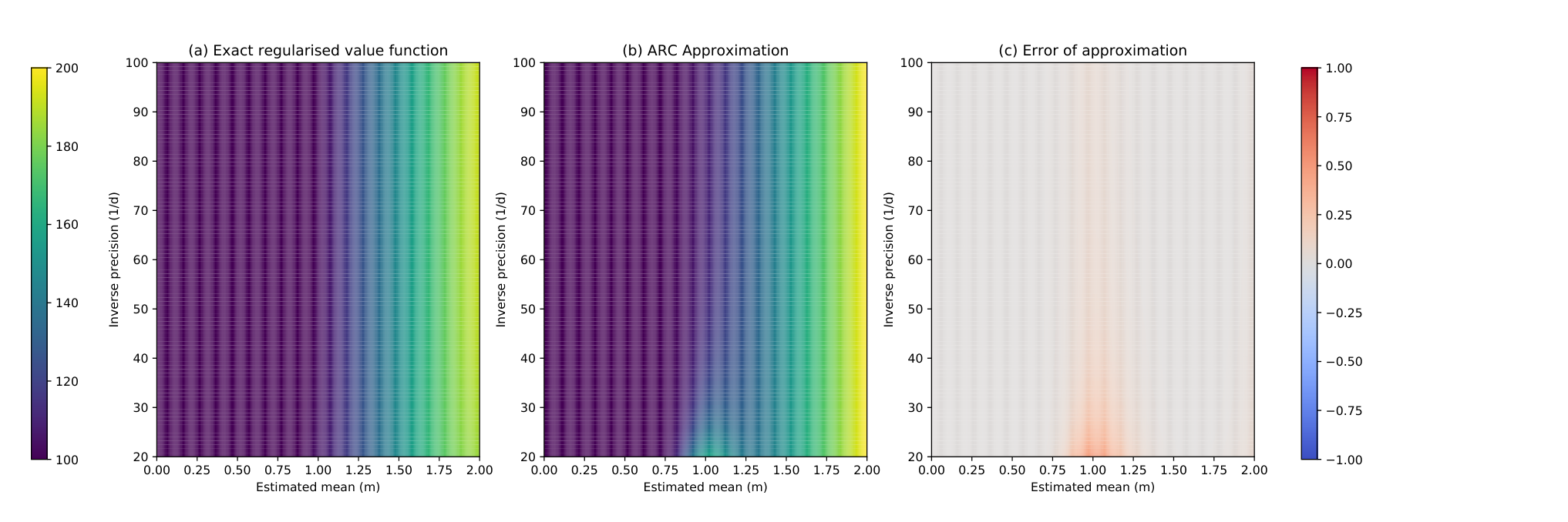
Suppose that our bandit has two arms. The first arm always gives the reward $Y\sim N(\theta,1)$ ; the second arm always gives reward $1$ . We observe the reward of the first arm only when the first arm is chosen. Formulating this as a relaxed control (2.13) with dynamic in (2.2) gives

V^{\lambda}_{\infty}(m,d)=\sup_{\varphi\in\Psi}{\mathbb{E}}_{m,d}\bigg[\sum_{t=0}^{\infty}\beta^{t}\Big(\big(U^{\varphi}_{1,t+1}M^{\varphi}_{t}+U^{\varphi}_{2,t+1}\big)+\lambda\mathcal{H}(U^{\varphi}_{t+1})\Big)\bigg]\quad;\quad\mathcal{H}(u)=-\sum_{i=1}^{2}u_{i}\ln u_{i}

with $\Theta={\mathbb{R}}$ and $\mathcal{D}=[0,1]$ . The transition (2.7) of the problem is given by

\Phi(m,d,i,\xi):=\begin{cases}(m,d)+\big(d(1+d)^{-1/2}z(\xi),-d^{2}(1+d)^{-1}\big)&;\;i=1\\ (m,d)&;\;i=2\end{cases}\quad\text{where}\;z(\bm{\xi}_{t})\sim_{IID}N(0,1).

We solve the above problem explicitly using Monte Carlo simulation. In particular, we start our iteration with $\tilde{V}^{\lambda}_{0}(m,d)=0$ and iteratively compute on the grid $(m,d)$ ,

\tilde{V}^{\lambda}_{n+1}(m,d)=\sup_{u\in\Delta^{2}}\Bigg\{u_{1}\Big(m+\frac{\beta}{N}\sum_{i=1}^{N}\tilde{V}^{\lambda}_{n}\big(\Phi(m,d,1,\bm{\xi}_{i,n})\big)\Big)+u_{2}\Big(1+\beta\tilde{V}^{\lambda}_{n}(m,d)\Big)+\lambda\mathcal{H}(u)\Bigg\}

where $N$ is the number of Monte Carlo simulations and $(\bm{\xi}_{i,n})$ are such that $z(\bm{\xi}_{i,n})\sim_{IID}N(0,1)$ . We then interpolate $\tilde{V}^{\lambda}_{n+1}$ and repeat the procedure until $\tilde{V}^{\lambda}_{n}$ converges to $\tilde{V}^{\lambda}$ . The corresponding optimal (feedback) probability to choose the first arm is given by

\tilde{p}^{\lambda,*}(m,d)\approx\frac{\exp\Big(\tfrac{1}{\lambda}\Big(m+\beta\big(\frac{1}{N}\sum_{i=1}^{N}\tilde{V}^{\lambda}(\Phi(m,d,1,\bm{\xi}_{i})\big)-\tilde{V}^{\bm{\lambda}}(m,d)\big)\Big)\Big)}{\exp\Big(\tfrac{1}{\lambda}\Big(m+\beta\big(\frac{1}{N}\sum_{i=1}^{N}\tilde{V}^{\lambda}(\Phi(m,d,1,\bm{\xi}_{i})\big)-\tilde{V}^{\bm{\lambda}}(m,d)\big)\Big)+\exp\big(\tfrac{1}{\lambda}\big)},

where $z(\bm{\xi}_{i})\sim_{IID}N(0,1)$ . On the other hand, our ARC approximation gives

V^{\lambda,ARC}_{\infty}(m,d)=(1-\beta)^{-1}\lambda\log\Big(\exp\Big(\frac{\alpha_{1}^{{\lambda}}(m,d)}{\lambda}\Big)+\exp\Big(\frac{1}{\lambda}\Big)\Big),\hskip 9.24994ptp^{\lambda,ARC}(m,d)=\frac{\exp\big(\frac{\alpha_{1}^{{\lambda}}(m,d)}{\lambda}\big)}{\exp\big(\frac{\alpha_{1}^{{\lambda}}(m,d)}{\lambda}\big)+\exp\big(\frac{1}{\lambda}\big)},

where $\alpha_{1}^{\lambda}(m,d)=m+\tfrac{1}{2\lambda}\beta(1-\beta)^{-1}\nu_{1}^{\lambda}(m)(1-\nu_{1}^{\lambda}(m))d^{2}(1+d)^{-1}$ and $\nu_{1}^{\lambda}(m)=\frac{\exp(m/\lambda)}{\exp(m/\lambda)+\exp(1/\lambda)}$ .

We now compare $\tilde{V}^{\lambda},\tilde{p}^{\lambda,*}$ with $V^{\lambda,ARC}_{\infty},p^{\lambda,ARC}$ when $\lambda=0.1$ and $\beta=0.99$ . In the numerical experiment, we use $N=1000$ and consider $m\in[0,2]$ and $d\in[1/100,1/20]$ . We see in Figure 1 (which shows the value functions) and Figure 2 (which shows the probability of choosing the risky arm) that the ARC approximation gives a close estimate of the regularised problem.

Refer to caption — Figure 1: (a) $\tilde{V}^{\lambda}\hskip 18.49988pt$ (b) $V^{\lambda,ARC}_{\infty}\hskip 18.49988pt$ (c) $(V^{\lambda,ARC}_{\infty}-\tilde{V}^{\lambda})/\tilde{V}^{\lambda}$

4.2 Simulation results

A common performance measure which is used in the multi-armed bandit literature [26, 11, 4, 16, 18] is the regret

R(A,T,\bm{\theta})=\sum_{t=1}^{T}\Big(\max_{i\in[K]}\mathbb{E}\big[R^{(i)}(Y^{(i)})\big|\bm{\theta}\big]-\mathbb{E}\big[R^{(A_{t})}(Y^{(A_{t})})\big|\bm{\theta}\big]\Big).

In this section, we will compare the regret of the ARC algorithm with other approaches described in Section 3.1 under $3$ environments; classical bandit, bandit with an informative arm and linear bandit. In each of these environments, we consider decisions on a $50$ -armed bandit with horizon $T=2\times 10^{3}$ steps over $10^{3}$ simulations. In the $n$ -th simulation, we sample the true parameter $\bm{\theta}^{(n)}\sim N(\bm{1}_{50},I_{50})$ and then simulate interaction between each of the algorithms and the environment with the parameter $\bm{\theta}^{(n)}$ starting from an initial belief $(m_{0},d_{0})=(0,10^{3}\times I_{50})$ corresponding to a non-informative prior. We then use our simulated output to demonstrate means, medians, 0.75 quantiles and 0.90 quantiles of the map $t\mapsto R(A,t,\bm{\theta})$ for each of our considered algorithms.

Simulation Environment:

We consider the following environment for our simulation. Let $\bm{\theta}$ be an unknown parameter taking values in ${\mathbb{R}}^{50}$ .

•

Classical bandit. When choosing the $i$ -th arm, we observe and receive the reward sampled from the distribution $N(\bm{\theta}_{i},5)$ .
•

Bandit with an informative arm. When choosing the $i$ -th arm with $i\neq 1$ , we observe and receive the reward sampled from the distribution $N(\bm{\theta}_{i},5)$ . When the $1$ -st arm is chosen, we receive a reward sampled from $N(\bm{\theta}_{1}-1,5)$ and in addition, we observe a sample from $N(\bm{\theta},5\times I_{50})$ . In particular, playing the first arm allows us to observe the rewards of other arms without choosing them, but this arm yields a smaller reward than others.
•

Linear bandit. When choosing the $i$ -th arm, we observe and receive a reward sampled from the distribution $N(b_{i}^{\top}\bm{\theta},5)$ where $b_{i}=e_{i}+e_{i+1}$ for $i\neq 50$ and $b_{50}=e_{1}+e_{50}$ .

Hyper-parameters of bandit algorithms:

We will consider the KG and IDS by introducing $100$ Monte-Carlo samples to evaluate the required expectations. We will set the parameter $\beta=0.9995$ for KG and ARC. The function $\bm{\lambda}(m,d)$ considered in the BE and ARC will be given in the form $\bm{\lambda}(m,d)=\rho\|d\|_{op}$ where $\|\cdot\|_{op}$ is the matrix operator norm and use Shannon entropy (Remark 2.3) to regularise the ARC algorithm. Unmentioned hyper-parameters will appear as a description of the algorithm in the regret plot.

ARC index strategy:

For numerical efficiency, we introduce an index strategy inspired by the ARC algorithm. In contrast to the ARC, instead of making a decision based on the probability simplex $\nu^{\bm{\lambda}(m,d)}\big(\alpha^{\bm{\lambda}(m,d)}(m,d)\big)$ with $\alpha^{\lambda}(m,d)$ given in (2.18), we simply choose the arm $i$ which maximises $\alpha_{i}^{\bm{\lambda}}(m,d)$ .

Figure 3: Regret for the classical bandit

Figure 4: Regret for the bandit with an informative arm

Figure 5: Regret for the linear bandit (IDS excluded due to computational cost)

Discussion of numerical simulations:

We see in Figures 3, 4 and 5 that both ARC and ARC index strategy with appropriate hyper-parameter perform very well compared to other algorithms. We see that the ARC approaches perform significantly better than other approaches in the setting for the bandit with an informative arm. This performance is as good as IDS but requires significantly lower computational cost, since every term can be evaluated explicitly. In fact, the computational cost of the IDS proved too expensive to demonstrate for the linear bandit with $50$ arms and was therefore omitted.

The ARC algorithm derived in this paper performs well with appropriate hyper-parameter choices. It is also worth pointing out one obstacle found in the derived ARC algorithm when running numerical simulations with many arms available. We see that taking $\bm{\lambda}(m,d)=\rho\|d\|$ may not allow $\|d\|$ to decay sufficiently fast (even though Theorem 2.3 ensures that this ultimately converges to $0$ ). In particular, with many arms, we should be able to identify some arms which are significantly worse than the others. Such arms will be rarely played, which leaves $\|d\|$ large for a long time. We found in the numerical simulation that when following the ARC procedure, the agent identifies the reward of the very best few arms correctly (i.e. we obtain close estimates to the rewards of a few best arms). Unfortunately, since $\|d\|$ does not decay sufficiently fast, this leads the ARC algorithm to randomly choose among some small number of options, even if it identifies the best arm correctly. This explains why we observe linear trends in the regret plot for the simple ARC but with a low gradient.

To overcome this effect, we considered the ARC index strategy, which does not require $\|d\|$ to decay to zero to terminate decision to a single (best) arm. Here, we see in Figure 3, 4 and 5 that the gradient of the regret of the ARC index converges to zero, that is, we eventually identify the best arm. In general, one may also choose the function $\bm{\lambda}(m,d)$ depending on $m$ to truncate our consideration to the best arm.

5 Proof of the main results

5.1 Convex analysis and smooth max approximator

In (2.11) and (2.12), we briefly introduce $\smaxld$ and $\nu^{\lambda}$ as a smooth version of the maximum function and its derivative, obtained via the convex conjugation of the regularisation function $\mathcal{H}$ . One well-known choice of $\mathcal{H}$ which gives an analytical expression is the Shannon entropy. We can also consider other choices of $\mathcal{H}$ by constructing the smooth max approximator $\smaxld$ explicitly⁶⁶ 6 Examples of explicit constructions can be found in Zhang and Reisinger [21, Remark 3.1]..

We observe that $\smaxld$ in (2.11) can be expressed as $\smaxld(a)=\lambda S(a/\lambda)$ where

S(a)=\sup_{u\in\Delta^{K}}\Big(\sum_{i=1}^{K}u_{i}a_{i}+\mathcal{H}(u)\Big).

(5.1)

In particular, $-\mathcal{H}$ is the convex conjugate of $S$ (see e.g. Rockafellar [22]). In fact, (5.1) is also known as a ‘nonlinear expectation’ ⁷⁷ 7 Nonlinear Expectations (or equivalently ‘risk measures’) are a classical tool in mathematical finance to study decision making under uncertainty. defined on a finite space (see Coquet et al. [9]).

Definition 5.1.

We say a function $S:\mathbb{R}^{K}\rightarrow\mathbb{R}$ is a convex nonlinear expectation if it satisfies:

1.

Monotonicity: If $a\leq b$ , then $S(a)\leq S(b)$ ;
2.

Translation Equivariance: For all $c\in\mathbb{R}$ , $S(a+c\bm{1}_{K})=S(a)+c$ ;
3.

Convexity: For any $\kappa\in[0,1]$ , $S(\kappa a+(1-\kappa)b)\leq\kappa S(a)+(1-\kappa)S(b)$ ;

where the inequalities are interpreted component-wise.

The following theorem shows that using $\smaxld$ as a smooth max approximator is equivalent to having $\mathcal{H}$ bounded. This will allow us to quantify the difference between a non-regularised (2.8) and regularised control problem (2.13) by $\mathcal{O}(\lambda)$ . The proof is given in Appendix A.

Theorem 5.1.

Let $S$ be a convex nonlinear expectation. The following are equivalent.

1.

There exists $N\in\mathbb{R}$ such that $S(a)+N\geq\max_{i}a_{i}$ for all $a\in\mathbb{R}^{K}$ .
2.

There exists $N\in\mathbb{R}$ such that $\mathcal{A}_{S}:=\{a\in\mathbb{R}^{K}:S(a)\leq 0\}\subseteq(-\infty,N]^{K}$ .
3.

There exists a bounded function $\mathcal{H}:\Delta^{K}\rightarrow\mathbb{R}$ such that (5.1) holds.
4.

For $\smaxld(a)=\lambda S(a/\lambda)$ , we have $\sup_{a\in\mathbb{R}}|\smaxld(a)-\max_{i}a_{i}|\rightarrow 0$ as $\lambda\downarrow 0$ .

We now introduce a smooth entropy regulariser as the convex conjugate of a smooth max approximator.

Definition 5.2.

We say a function $S:\mathbb{R}^{K}\rightarrow\mathbb{R}$ is a smooth max approximator if it is a $3$ -times differentiable convex nonlinear expectation with uniformly bounded derivatives such that Theorem 5.1 holds. We say a bounded function $\mathcal{H}:\Delta^{K}\rightarrow\mathbb{R}$ is a smooth entropy if $-\mathcal{H}$ is a convex conjugate of some smooth max approximator⁸⁸ 8 One can check that the Shannon Entropy (Remark 2.3) is a smooth entropy..

For a smooth max approximator $S$ , we write $\smaxld(a):=\lambda S(a/\lambda)$ , $\nu^{\lambda}(a):=\partial_{y}S\big|_{y=a/\lambda}=\partial_{a}\smaxld(a)$ and $\eta^{\lambda}(a):=\partial^{2}_{y}S\big|_{y=a/\lambda}=\lambda\partial^{2}_{a}\smaxld(a)$ .

Remark 5.1.

If $S$ is a smooth max approximator, then $\nu^{\lambda}$ and $\eta^{\lambda}$ are uniformly bounded. Moreover, it follows from Fenchel’s inequality that $\nu^{\lambda}(a)=\argmax_{u\in\Delta^{K}}\big(\sum_{i=1}^{K}u_{i}a_{i}+\lambda\mathcal{H}(u)\big).$ In particular, $\nu^{\lambda}$ can be interpreted as a smooth version of the argmax, as in (2.12).

5.2 Analysis of the regularised control problem over finite horizon

The objective of this section is to approximate the finite horizon value function as a sum of the (smooth) maximum of the incremental rewards.

Definition 5.3.

Let $\mathcal{H}:\Delta^{K}\rightarrow\mathbb{R}$ be a smooth entropy (Definition 5.2) and $\lambda>0$ . Define

\left.\begin{aligned} V^{\lambda}_{T}(m,d)&:=\sup_{\varphi\in\Psi}V^{\lambda,\varphi}_{T}(m,d),\qquad\text{where}\\ V^{\lambda,\varphi}_{T}(m,d)&:=\mathbb{E}_{m,d}\Bigg[\sum_{t=0}^{T-1}\beta^{t}\bigg(\Big(\sum_{i=1}^{K}f_{i}\big(M^{\varphi}_{t},D^{\varphi}_{t}\big)U^{\varphi}_{i,t+1}\Big)+\lambda\mathcal{H}(U^{\varphi}_{t+1})\bigg)\Bigg].\end{aligned}\right\}

(5.2)

We will show that $V^{\lambda}_{T}(m,d)\approx\sum_{t=0}^{T-1}\beta^{t}\big(\smaxld\circ\alpha_{T-t}^{\lambda}\big)(m,d)$ , with an approximate optimal policy $\varphi^{\lambda,T}(t,m,d):=\nu^{\lambda}\big(\alpha^{\lambda}_{T-t+1}(m,d)\big)$ . Here, the incremental reward with $t$ -steps to go is

\alpha_{t}^{\lambda}(m,d):=f(m,d)+L^{\lambda}(m,d)\bigg(\sum_{s=1}^{t-1}\beta^{s}\bigg),

(5.3)

where $L^{\lambda}(m,d)$ is given in (2.19).

The idea behind the analysis is to consider an asymptotic expansion as $\|d\|\rightarrow 0$ . Due to our learning structure (H.2), the change in the underlying state $(m,d)$ are (in expectation) of order $\mathcal{O}(\|d\|^{2})$ . Hence, the global Lipschitz property of $f$ implies that the instantaneous reward changes with $\mathcal{O}(\|d\|^{2})$ . Hence, we can use Taylor’s theorem to obtain an asymptotic expansion in $\|d\|$ and keep the terms up to order $\mathcal{O}(\|d\|^{2})$ .

We first show that the perturbation error in the learning term $L^{\lambda}$ is of order $\mathcal{O}(\|d\|^{3})$ and can be ignored in our approximation. The proofs of the following two lemmas are in Appendix A.

Lemma 5.2.

Suppose that (H.1) and (H.2) hold, and let $S$ be a smooth max approximator (Definition 5.2). There exists a constant $C>0$ such that the function $(\lambda,m,d)\mapsto L^{\lambda}(m,d)$ given in (2.19) satisfies: for any $\lambda>0$ , $i\in[K]$ , $(m,d)\in\Theta\times\mathcal{D}$ and $t\in{\mathbb{N}}$ ,

{\mathbb{E}}\big|L^{\lambda}\big(\Phi(m,d,i,\bm{\xi}_{t})\big)-L^{\lambda}(m,d)\big|\leq C\|d\|^{3}(1+\lambda^{-2}).

Now, we consider the second order approximation of the smooth maximum $\smaxld$ over the incremental reward $\alpha$ . We show that $L^{\lambda}$ is the second order approximation (in expectation) of the (smooth) maximum incremental reward.

Lemma 5.3.

Suppose that (H.1) and (H.2) hold , and let $S$ be a smooth max approximator (Definition 5.2) and $\smaxld(a):=\lambda S(a/\lambda)$ . There exists a constant $C>0$ such that for any $\lambda>0$ , $i\in[K]$ , $(m,d)\in\Theta\times\mathcal{D}$ and $t,T\in{\mathbb{N}}$ ,

\displaystyle\Big|{\mathbb{E}}\big(\smaxld\circ\alpha_{T}^{\lambda}\big)\big(\Phi(m,d,i,\bm{\xi}_{t})\big)-\big(\smaxld\circ\alpha_{T}^{\lambda}\big)(m,d)-L_{i}^{\lambda}(m,d)\Big|\leq C\|d\|^{3}\big(1+\lambda^{-2}+\lambda^{-3}\|d\|\big)

where $\alpha^{\lambda}_{t}$ is defined in (5.3), $L^{\lambda}$ is defined in (2.19).

Since $\alpha^{\lambda}_{t}(m,d)$ describes an incremental reward with $t$ -steps to go, we may approximate the optimal value function (5.2) by $\sum_{t=0}^{T-1}\beta^{t}\big(\smaxld\circ\alpha_{T-t}^{\lambda}\big)(m,d)$ with an estimate optimal strategy $\varphi^{\lambda,T}(t,m,d):=\nu^{\lambda}\big(\alpha^{\lambda}_{T-t}(m,d)\big)$ .

Theorem 5.4.

Suppose that (H.1) and (H.2) hold, and let $S$ be a smooth max approximator (Definition 5.2) and $\smaxld(a):=\lambda S(a/\lambda)$ . There exists a constant $C>0$ such that the value function for finite horizon (Definition 5.3) satisfies: for any $\lambda>0$ , $(m,d)\in\Theta\times\mathcal{D}$ and $T\in{\mathbb{N}}$ ,

	$\displaystyle\Big\|V^{\lambda,\varphi^{\lambda,T}}_{T}(m,d)-\sum_{t=0}^{T-1}\beta^{t}\big(\smaxld\circ\alpha_{T-t}^{\lambda}\big)(m,d)\Big\|$	$\displaystyle\leq C\\|d\\|^{3}\big(1+\lambda^{-2}+\lambda^{-3}\\|d\\|\big),\quad\text{and}$		(5.4)
	$\displaystyle\Big\|V^{\lambda}_{T}(m,d)-\sum_{t=0}^{T-1}\beta^{t}\big(\smaxld\circ\alpha_{T-t}^{\lambda}\big)(m,d)\Big\|$	$\displaystyle\leq C\\|d\\|^{3}\big(1+\lambda^{-2}+\lambda^{-3}\\|d\\|\big).$		(5.5)

where $\varphi^{\lambda,T}(t,m,d):=\nu^{\lambda}\big(\alpha^{\lambda}_{T-t+1}(m,d)\big)=\partial_{a}\smaxld\big(\alpha^{\lambda}_{T-t+1}(m,d)\big)$ and $\alpha^{\lambda}_{t}$ is defined in (5.3).

Proof.

We will prove by induction that the upper-bounds for (5.4) and (5.5) are given by $Q_{\lambda,d}=(1-\beta)^{-2}C\|d\|^{3}\big(1+\lambda^{-2}+\lambda^{-3}\|d\|\big)$ where $C\geq 0$ is a constant in Lemma 5.3.

It is clear from (2.11) that $V^{\lambda}_{1}=\smaxld\circ\alpha_{1}^{\lambda}$ . Hence, the required inequality holds for $T=1$ .

Assume that the required inequality holds for $T-1$ .

Define $R^{i}_{T}(m,d):=\beta\mathbb{E}\big[V^{\lambda,\varphi^{\lambda,T-1}}_{T-1}\big(\Phi(m,d,i,\bm{\xi}_{1})\big)\big]-\sum_{t=1}^{T-1}\beta^{t}\left(\big(\smaxld\circ\alpha_{t}^{\lambda}\big)(m,d)+L_{i}^{\lambda}(m,d)\right).$ We see that

		$\displaystyle V_{T}^{\lambda,\varphi^{\lambda,T}}(m,d)=\sum_{i=1}^{K}U^{\varphi^{\lambda,T},m,d}_{i,1}\Big(f_{i}(m,d)+\beta\mathbb{E}\big[V_{T-1}^{\lambda,\varphi^{\lambda,T-1}}\big(\Phi(m,d,i,\bm{\xi}_{1})\big)\big]\Big)+\lambda\mathcal{H}(U^{\varphi^{\lambda,T},m,d}_{1})$
		$\displaystyle\quad=\bigg(\sum_{i=1}^{K}U^{\varphi^{\lambda,T},m,d}_{i,1}\Big(\alpha^{\lambda}_{T,i}(m,d)+R^{i}_{T}(m,d)\Big)+\lambda\mathcal{H}(U^{\varphi^{\lambda,T},m,d}_{1})\bigg)+\sum_{t=1}^{T-1}\beta^{t}\big(\smaxld\circ\alpha^{\lambda}_{T-1-t}\big)(m,d)$
		$\displaystyle\quad=\bigg(\sum_{i=1}^{K}U^{\varphi^{\lambda,T},m,d}_{i,1}R^{i}_{T}(m,d)\bigg)+\big(\smaxld\circ\alpha^{\lambda}_{T}\big)(m,d)+\sum_{t=1}^{T-1}\beta^{t}\big(\smaxld\circ\alpha^{\lambda}_{T-1-t}\big)(m,d)$		(5.6)

where the second equality follows from substituting $\alpha^{\lambda}_{T,i}(m,d)=f_{i}(m,d)+\beta\big(\sum_{t=1}^{T-1}\beta^{t}\big)L_{i}^{\lambda}(m,d)$ and the final inequality follows from (2.11)-(2.12) and the fact that

U^{\varphi^{\lambda,T},m,d}_{1}=\partial_{a}\smaxld\big(\alpha^{\lambda}_{T}(m,d)\big)=\argmax_{u\in\Delta^{K}}\bigg(\sum_{i=1}^{K}u_{i}\alpha^{\lambda}_{T,i}(m,d)+\lambda\mathcal{H}(u)\bigg).

By our inductive hypothesis, Lemma 5.3 and (H.2) $(i)$ , we see that

	$\displaystyle\|R^{i}_{T}(m,d)\|$	$\displaystyle:=\beta\mathbb{E}\left\|V^{\lambda,\varphi^{\lambda,T-1}}_{T-1}\big(\Phi(m,d,i,\bm{\xi}_{1})\big)-\sum_{t=0}^{T-2}\beta^{t}\big(\smaxld\circ\alpha_{T-t}^{\lambda}\big)\big(\Phi(m,d,i,\bm{\xi}_{1})\big)\right\|$
		$\displaystyle\qquad+\sum_{t=0}^{T-2}\beta^{t}\left\|{\mathbb{E}}\big[\big(\smaxld\circ\alpha_{t}^{\lambda}\big)\big(\Phi(m,d,i,\bm{\xi}_{1})\big)\big]-\big(\smaxld\circ\alpha_{t}^{\lambda}\big)(m,d)-L_{i}^{\lambda}(m,d)\right\|$
		$\displaystyle\leq\beta Q_{\lambda,d+b_{i}(m,d)}+\Big(\sum_{t=0}^{T-2}\beta^{t}\Big)(1-\beta)^{2}Q_{\lambda,d}\leq\beta Q_{\lambda,d}+(1-\beta)Q_{\lambda,d}=Q_{\lambda,d}.$

Therefore, $\big|\sum_{i=1}^{K}U^{\varphi^{\lambda,T},m,d}_{i,1}R^{i}_{T}(m,d)\big|\leq Q_{\lambda,d}$ and the inequality (5.4) for $T$ follows from (5.2).

Similarly, to prove (5.5), we define $\tilde{R}^{i}_{T}(m,d)$ in the same manner as ${R}^{i}_{T}(m,d)$ but replace $V^{\lambda,\varphi^{\lambda,T-1}}_{T-1}$ by $V^{\lambda}_{T-1}$ . The similar argument yields $|\tilde{R}^{i}_{T}(m,d)|\leq Q_{\lambda,d}$ for all $T\in{\mathbb{N}}$ and $i\in[K]$ .

It follows from the dynamic programming principle that

		$\displaystyle V_{T}^{\lambda}(m,d)=\sup_{u\in\Delta^{K}}\bigg\{\sum_{i=1}^{K}u_{i}\Big(f_{i}(m,d)+\beta\mathbb{E}\big[V^{\lambda}_{T-1}\big(\Phi(m,d,i,\bm{\xi}_{1})\big)\big]\Big)+\lambda\mathcal{H}(u)\bigg\}$
		$\displaystyle\quad=\sup_{u\in\Delta^{K}}\bigg\{\bigg(\sum_{i=1}^{K}u_{i}\alpha^{\lambda}_{T,i}(m,d)+\lambda\mathcal{H}(u)\bigg)+\bigg(\sum_{i=1}^{K}u_{i}\tilde{R}^{i}_{T}(m,d)\bigg)\bigg\}+\sum_{t=1}^{T-1}\beta^{t}\big(\smaxld\circ\alpha^{\lambda}_{T-1-t}\big)(m,d).$

Since $\sup_{u\in\Delta^{K}}\big|\sum_{i=1}^{K}u_{i}\tilde{R}^{i}_{T}(m,d)\big|\leq Q_{\lambda,d}$ , the inequality (5.2) for $T$ follows from (2.11). ∎

5.3 Analysis of the regularised control problem over infinite horizon

We see that the error bound of our approximation in Theorem 5.4 is uniform in $T$ . We can now prove Theorem 2.1 by taking $T\rightarrow\infty$ in Theorem 5.4.

Proof of Theorem 2.1.

Fix $(m,d)\in\Theta\times\mathcal{D}$ and $\lambda>0$ .

Since $(\smaxld\circ\alpha^{\lambda}_{t}\big)(m,d)\rightarrow(\smaxld\circ\alpha^{\lambda}\big)(m,d)$ as $t\rightarrow\infty$ , it follows from a Tauberian theorem (Theorem A.2) that

\sum_{t=0}^{T-1}\beta^{t}\big(\smaxld\circ\alpha_{T-t}^{\lambda}\big)(m,d)\rightarrow(1-\beta)^{-1}\big(\smaxld\circ\alpha^{\lambda}\big)(m,d)\qquad\text{as }T\rightarrow\infty.

(5.7)

Next, we will prove that $V^{\lambda}_{T}(m,d)\rightarrow V^{\lambda}_{\infty}(m,d)$ as $T\rightarrow\infty$ . By (H.2) together with the Cauchy–Schwarz inequality, we can show that for any $\varphi\in\Psi$ , ${\mathbb{E}}_{m,d}|M^{\varphi}_{t+1}-M^{\varphi}_{t}|\leq C\|D^{\varphi}_{t}\|\leq C\|d\|$ . In particular, ${\mathbb{E}}_{m,d}|M^{\varphi}_{t}|\leq|m|+CT\|d\|$ . By (H.1), there exists a constant $C\geq 0$ , such that

\left.\begin{aligned} &\sup_{\varphi\in\Psi}\sum_{t=T}^{\infty}\beta^{t}{\mathbb{E}}_{m,d}\bigg[\bigg|\sum_{i=1}^{K}f_{i}\big(M^{\varphi}_{t},D^{\varphi}_{t}\big)U^{\varphi}_{i,t+1}\bigg|\bigg]\leq C\sup_{\varphi\in\Psi}\sum_{t=T}^{\infty}\beta^{t}{\mathbb{E}}_{m,d}\big[|M^{\varphi}_{t}|+\|d\|+1\big]\\ &\hskip 142.26378pt\leq C\sum_{t=T}^{\infty}\beta^{t}\big((t+1)\|d\|+|m|+1\big)\rightarrow 0\qquad\text{as}\quad T\rightarrow\infty.\end{aligned}\right\}

(5.8)

Moreover, since $\mathcal{H}$ is a smooth entropy, $\mathcal{H}$ is bounded and so $\sup_{U\in\mathcal{U}}\sum_{t=T}^{\infty}\beta^{t}{\mathbb{E}}_{m,d}\big[|\mathcal{H}(U^{\varphi}_{t+1})|\big]\rightarrow 0$ as $T\rightarrow 0$ . Combining this with (5.8), we obtain

\Big|V_{T}^{\lambda}(m,d)-V^{\lambda}_{\infty}(m,d)\Big|\leq\sup_{\varphi\in\Psi}\bigg|\mathbb{E}_{m,d}\bigg[\sum_{t=T}^{\infty}\beta^{t}\Big(\sum_{i=1}^{K}f_{i}\big(M^{\varphi}_{t},D^{\varphi}_{t}\big)U^{\varphi}_{i,t+1}+\lambda\mathcal{H}(U^{\varphi}_{t+1})\Big)\bigg]\bigg|\rightarrow 0\;\text{as}\;T\rightarrow\infty.

(5.9)

Next, we will prove that $V^{\lambda,\varphi^{\lambda,T}}_{T}(m,d)\rightarrow V^{\lambda,\varphi^{\lambda}}(m,d)$ where $\varphi^{\lambda,T}(t,m,d):=\partial_{a}\smaxld\big(\alpha^{\lambda}(m,d)\big)$ and $\varphi^{\lambda,T}(t,m,d):=\partial_{a}\smaxld\big(\alpha^{\lambda}_{T-t+1}(m,d)\big)$ with $\alpha$ and $\alpha_{t}$ given (2.18) and (5.3), respectively.

For any policy $\varphi\in\Psi$ , let $g(t;\varphi):=\mathbb{E}_{m,d}\big[\big(\sum_{i=1}^{K}f_{i}\big(M^{\varphi}_{t},D^{\varphi}_{t}\big)U^{\varphi}_{i,t+1}\big)+\lambda\mathcal{H}(U^{\varphi}_{t+1})\big]$ . By the similar argument as in (5.8), we can find a constant $C\geq 0$ such that $\sup_{\varphi\in\Psi}g(t;\varphi)\leq C\big((t+1)\|d\|+|m|+1\big)$ . Since $V^{\lambda,\varphi^{\lambda,T}}_{T}(m,d)=\sum_{t=0}^{T-1}\beta^{t}g(t;\varphi^{\lambda,T})$ and $V^{\lambda,\varphi^{\lambda}}(m,d)=\sum_{t=0}^{\infty}\beta^{t}g(t;\varphi^{\lambda})$ , it suffices to show that for any fixed $t\in{\mathbb{N}}$ , $g(t;\varphi^{\lambda,T})\rightarrow g(t;\varphi^{\lambda})$ as $T\rightarrow\infty$ . Given this, the required convergence follows from a Tauberian theorem (Theorem A.3).

Fix $t\in{\mathbb{N}}$ . By (H.1) and (H.2), there exists a constant $C\geq 0$ such that $\big|L^{\lambda}(M^{\varphi^{\lambda},m,d}_{s},D^{\varphi^{\lambda},m,d}_{s})\big|\leq C$ for all $s\in{\mathbb{N}}$ . For any $s=1,2,...,t$ , it follows from the mean value inequality that

\left.\begin{aligned} &\Big|\nu^{\lambda}\big(\alpha^{\lambda}(M^{\varphi^{\lambda},m,d}_{s},D^{\varphi^{\lambda},m,d}_{s})\big)-\nu^{\lambda}\big(\alpha_{T-s+1}^{\lambda}(M^{\varphi^{\lambda},m,d}_{s},D^{\varphi^{\lambda},m,d}_{s})\big)\Big|\\ &\qquad\leq\|\partial_{a}\nu^{\lambda}\|_{\infty}\Big(\sum_{r=T-s+1}^{\infty}\beta^{r}\Big)\big|L^{\lambda}(M^{\varphi^{\lambda},m,d}_{s},D^{\varphi^{\lambda},m,d}_{s})\big|\\ &\qquad\leq C\|\partial_{a}\nu^{\lambda}\|_{\infty}\beta^{T-s+1}(1-\beta)^{-1}\leq C\|\partial_{a}\nu^{\lambda}\|_{\infty}\beta^{T-t+1}(1-\beta)^{-1}.\end{aligned}\right\}

(5.10)

Fix $\epsilon\in(0,1)$ and choose $T_{0}$ such that, for all $T\geq T_{0}$ , we have $C\|\partial_{a}\nu^{\lambda}\|_{\infty}\beta^{T-t+1}(1-\beta)^{-1}<\epsilon/K$ .

As discussed in Section 2.2, we recall that the action corresponding to the policy $\varphi$ is given by $A^{\varphi,m,d}_{s}=\sup\big\{i:\sum_{k=1}^{i}U^{\varphi,m,d}_{s,k}\geq\zeta_{s}\big\}$ . By (5.10), for $T\geq T_{0}$ , the probability that the actions corresponding to $\varphi^{\lambda}$ and $\varphi^{\lambda,T}$ disagree at time $s$ , provided they agree up to time $s-1$ , satisfies

		$\displaystyle\mathbb{P}(A^{\varphi^{\lambda},m,d}_{s}\neq A^{\varphi^{\lambda,T},m,d}_{s}\|A^{\varphi^{\lambda},m,d}_{r}=A^{\varphi^{\lambda,T},m,d}_{r}\;\forall r=1,2,...,s-1)$
		$\displaystyle\qquad\qquad\leq\sum_{i=1}^{K}\Big\|\nu_{i}^{\lambda}\big(\alpha^{\lambda}(M^{\varphi^{\lambda},m,d}_{s},D^{\varphi^{\lambda},m,d}_{s})\big)-\nu_{i}^{\lambda}\big(\alpha_{T-s}^{\lambda}(M^{\varphi^{\lambda},m,d}_{s},D^{\varphi^{\lambda},m,d}_{s})\big)\Big\|\leq\epsilon.$

Let $E_{T}$ be the the event that the actions corresponding to $\varphi^{\lambda}$ and $\varphi^{\lambda,T}$ agree up to time $t$ , i.e. $E_{T}:=\{A^{\varphi^{\lambda},m,d}_{s}=A^{\varphi^{\lambda,T},m,d}_{s}\;\forall s=1,...,t\}$ . This gives $\mathbb{P}(E_{T})\geq(1-\epsilon)^{t}\geq 1-t\epsilon$ , i.e. $\mathbb{P}(E_{T}^{c})\leq t\epsilon$ .

By (H.1) and (H.2), we can find a constant $C\geq 0$ such that for any $\varphi\in\Psi$ ,

{\mathbb{E}}_{m,d}|f\big(M^{\varphi}_{t},D^{\varphi}_{t}\big)|^{2}\leq Ct(|m|^{2}+\|d\|^{2}+1).

Moreover, as $\mathcal{H}$ is bounded, we can assume (wlog) that $\sup_{u\in\Delta^{K}}\mathcal{H}(u)\leq C$ .

Since $(M^{\varphi^{\lambda},m,d}_{t},D^{\varphi^{\lambda},m,d}_{t})=(M^{\varphi^{\lambda,T},m,d}_{t},D^{\varphi^{\lambda,T},m,d}_{t})$ and $U^{\varphi^{\lambda},m,d}_{t}=U^{\varphi^{\lambda,T},m,d}_{t}$ on $E_{T}$ , we see that

|g(t;\varphi^{\lambda,T})-g(t;\varphi^{\lambda})|\leq 2\sup_{\varphi\in\Psi}{\mathbb{E}}\Big[\big(|f(M^{\varphi}_{t},D^{\varphi}_{t})|+\lambda\mathcal{H}(U^{\Psi}_{t+1})\big){\mathbb{I}}_{E_{T}^{c}}\Big]\leq 4Ct(|m|^{2}+\|d\|^{2}+2)(t\epsilon)

where the final inequality follows from the Cauchy–Schwarz inequality. As $\epsilon$ is arbitrary, we obtain the required result that for any fixed $t\in{\mathbb{N}}$ , $g(t;\varphi^{\lambda,T})\rightarrow g(t;\varphi^{\lambda})$ as $T\rightarrow\infty$ which implies that

V^{\lambda,\varphi^{\lambda,T}}_{T}(m,d)\rightarrow V^{\lambda,\varphi^{\lambda}}(m,d)\qquad\text{as }T\rightarrow\infty.

(5.11)

Finally, combining (5.7), (5.9) and (5.11) with Theorem 5.4 gives the required error bound. ∎

5.4 Analysis of the (unregularised) control problem

This section is dedicated to prove Theorem 2.2.

Proof of Theorem 2.2.

Through the following argument, let $C\geq 0$ be a generic constant, depending only on $\beta$ and the bounds in (H.1) and (H.2) which could be different between lines.

We will first show that there exists a constant $\tilde{C}\geq 0$ such that

V(m,d)-Q\big(\varphi^{\bm{\lambda}}(1,m,d),m,d\big)\leq\tilde{C}(\|d\|^{3-2\kappa}+\|d\|^{4-3\kappa}+\|d\|^{\kappa}),

(5.12)

where $Q(u,m,d):=\sum_{i=1}^{K}u_{i}\big(f_{i}(m,d)+\beta{\mathbb{E}}\big[V\big(\Phi(m,d,i,\bm{\xi}_{1})\big)\big]\big)$ .

Observe that

V^{\bm{\lambda}(m,d),\varphi^{\bm{\lambda}(m,d)}}(m,d)=\sum_{i=1}^{K}\varphi_{i}^{\bm{\lambda}}(1,m,d)\bigg(f_{i}(m,d)+\beta{\mathbb{E}}\Big[V^{\bm{\lambda}(m,d),\varphi^{\bm{\lambda}(m,d)}}_{\infty}\big(\Phi(m,d,i,\bm{\xi}_{1})\big)\Big]\bigg)+\bm{\lambda}(m,d)\mathcal{H}\big(\varphi^{\bm{\lambda}}(1,m,d)\big)

and write

\left.\begin{aligned} &Q\big(\varphi^{\bm{\lambda}}(1,m,d),m,d\big)-V(m,d)\\ &\hskip 9.24994pt=\Big(V^{\bm{\lambda}(m,d),\varphi^{\bm{\lambda}(m,d)}}(m,d)-V^{\bm{\lambda}(m,d)}(m,d)\Big)+\Big(V^{\bm{\lambda}(m,d)}(m,d)-V(m,d)\Big)\\ &\hskip 9.24994pt\hskip 9.24994pt+\beta\sum_{i=1}^{K}\varphi_{i}^{\bm{\lambda}}(1,m,d){\mathbb{E}}\Big[V^{\bm{\lambda}(m,d)}_{\infty}\big(\Phi(m,d,i,\bm{\xi}_{1})\big)-V^{\bm{\lambda}(m,d),\varphi^{\bm{\lambda}(m,d)}}_{\infty}\big(\Phi(m,d,i,\bm{\xi}_{1})\big)\Big]\\ &\hskip 9.24994pt\hskip 9.24994pt+\beta\sum_{i=1}^{K}\varphi_{i}^{\bm{\lambda}}(1,m,d){\mathbb{E}}\Big[V\big(\Phi(m,d,i,\bm{\xi}_{1})\big)-V^{\bm{\lambda}(m,d)}_{\infty}\big(\Phi(m,d,i,\bm{\xi}_{1})\big)\Big]-\bm{\lambda}(m,d)\mathcal{H}\big(\varphi^{\bm{\lambda}}(1,m,d)\big)\end{aligned}\right\}

(5.13)

Since $\mathcal{H}$ is bounded, for any $\lambda>0$ , $\lambda|\mathcal{H}(u)|\leq C\lambda$ for all $u\in\Delta^{K}$ and $\big|V^{\lambda}(m,d)-V(m,d)\big|\leq C\lambda$ for all $(m,d)\in\Theta\times\mathcal{D}$ . Combining this observation with (5.13) and Theorem 2.1, we see that

\Big|Q\big(\varphi^{\bm{\lambda}}(1,m,d),m,d\big)-V(m,d)\Big|\leq C\bm{\lambda}(m,d)+C\|d\|^{3}\big(1+\bm{\lambda}(m,d)^{-2}+\bm{\lambda}(m,d)^{-3}\|d\|\big).

Since $\mathcal{D}$ is compact, $\|d\|^{3}\leq C\|d\|^{3-2\kappa}$ . Therefore, (5.12) follows from our assumption that $\underline{c}\|d\|^{\kappa}\leq\bm{\lambda}(m,d)\leq\bar{c}\|d\|^{\kappa}$ for some constant $\underline{c},\bar{c}>0$ .

Let $\varphi^{*}:{\mathbb{N}}\times\Theta\times\mathcal{D}\rightarrow\Delta^{K}$ be the optimal (stationary) feedback policy of (2.8), i.e. $V^{\varphi^{*}}=V$ . For each $N\in{\mathbb{N}}$ , let

\varphi^{\bm{\lambda},N}(t,m,d)=\begin{cases}\varphi^{\bm{\lambda}}(t,m,d)&;t=1,2,...,N\\ \varphi^{*}(t,m,d)&;\text{otherwise}\end{cases}.

We next show, by induction, that $V(m,d)-V^{\varphi^{\bm{\lambda},N}}(m,d)\leq\varepsilon(d)$ where $\varepsilon(d):=(1-\beta)^{-1}\tilde{C}(\|d\|^{3-2\kappa}+\|d\|^{4-3\kappa}+\|d\|^{\kappa})$ with the constant $\tilde{C}\geq 0$ given in (5.12).

It is clear from the definition of $\varphi^{\bm{\lambda},N}$ that the required inequality holds for $N=0$ . Assume that the required inequality holds for $N-1$ . Observe that

	$\displaystyle V^{\varphi^{\bm{\lambda},N}}(m,d)$	$\displaystyle=\sum_{i=1}^{K}\varphi_{i}^{\bm{\lambda}}(1,m,d)f_{i}(m,d)+\beta{\mathbb{E}}_{m,d}\big[V(M^{\varphi^{\bm{\lambda}}}_{1},D^{\varphi^{\bm{\lambda}}}_{1})\big]+\beta R_{N}(m,d)$
		$\displaystyle=Q\big(\varphi^{\bm{\lambda}}(1,m,d),m,d\big)+\beta R_{N}(m,d),$

where $R_{N}(m,d):={\mathbb{E}}_{m,d}\big[V^{\varphi_{N-1}^{\bm{\lambda}}}(M^{\varphi^{\bm{\lambda}}}_{1},D^{\varphi^{\bm{\lambda}}}_{1})-V(M^{\varphi^{\bm{\lambda}}}_{1},D^{\varphi^{\bm{\lambda}}}_{1})\big]$ . By the induction hypothesis and (H.2), $\|D^{\varphi^{\bm{\lambda}}}_{1}\|\leq\|d\|$ , and thus $|R_{N}(m,d)|\leq{\mathbb{E}}[\varepsilon(D^{\varphi^{\bm{\lambda}}}_{1})]\leq\varepsilon(d)$ . Hence, the induction step follows from (5.12).

The main inequality of this theorem follows from the fact that $V^{\varphi^{\bm{\lambda},N}}(m,d)\rightarrow V^{\varphi^{\bm{\lambda}}}(m,d)$ as $N\rightarrow\infty$ which can be proved in the similar manner as the proof that $V^{\lambda}_{T}(m,d)\rightarrow V^{\lambda}_{\infty}(m,d)$ as $T\rightarrow\infty$ in Theorem 2.1. ∎

5.5 Complete Learning

We have discussed in Section (3.2) that some bandit algorithms e.g. greedy or KG may suffer from incomplete learning. Theorem 2.3 show that the ARC algorithm overcomes this limitation, in the sense that $\|D^{\varphi^{\bm{\lambda}}}_{t}\|\rightarrow 0$ as $t\rightarrow\infty$ . This section is dedicated to prove this result.

Proof of Theorem 2.3.

By (H.1), (H.2) and the fact that $\bm{\lambda}(m,d)\geq\underline{c}\|d\|^{\kappa}$ , there exists a constant $C\geq 0$ such that $|L^{\bm{\lambda}(m,d)}(m,d)|\leq C\big(1+\bm{\lambda}(m,d)^{-1}\big)\|d\|^{2}\leq C(\|d\|^{2}+\|d\|^{2-\kappa}\underline{c}^{-1})$ . Since $\kappa\leq 2$ and $\mathcal{D}$ is compact, $L^{\bm{\lambda}(m,d)}(m,d)$ is uniformly bound on $\Theta\times\mathcal{D}$ . Combining this with the boundedness of $f$ yields $\sup_{(m,d)\in\Theta\times\mathcal{D}}|\alpha^{\bm{\lambda}(m,d)}(m,d)|\leq C$ for some constant $C\geq 0$ .

Fix $(m,d)\in\Theta\times\mathcal{D}$ , $i\in[K]$ and $\epsilon>0$ and consider the events $E_{\epsilon}:=\{\|D^{\varphi^{\bm{\lambda}},m,d}_{t}\|>\epsilon\quad\forall t\in{\mathbb{N}}\}$ , $F_{i}:=\{A^{\varphi^{\bm{\lambda}},m,d}_{s}=i\;\text{for finitely many }t\in{\mathbb{N}}\}$ and $G_{i,t}:=\{A^{\varphi^{\bm{\lambda}},m,d}_{t}\neq i\}$ .

For $\|d\|>\epsilon$ , $\alpha^{\bm{\lambda}(m,d)}(m,d)/\bm{\lambda}(m,d)$ takes values in a compact set. Hence, there exists $r\in(0,1)$ such that $\nu^{\bm{\lambda}(m,d)}_{i}\big(\alpha^{\bm{\lambda}(m,d)}(m,d)\big)=(\partial_{a}S)_{i}\big(\alpha^{\bm{\lambda}(m,d)}(m,d)/\bm{\lambda}(m,d)\big)>r$ for $\|d\|>\epsilon$ . In particular, for any $n,N\in{\mathbb{N}}$ , $\mathbb{P}\big(\bigcap_{t=n}^{N}G_{i,t}\big|E_{\epsilon}\big)=\prod_{t=n}^{N}\mathbb{P}\big(G_{i,t}\big|E_{\epsilon}\cap\bigcap_{s=n}^{t-1}G_{i,s}\big)\leq(1-r)^{N-n+1}\rightarrow 0$ as $N\rightarrow\infty$ . Therefore,

\mathbb{P}(F_{i}\cap E_{\epsilon})=\mathbb{P}(E_{\epsilon})\mathbb{P}(F_{i}|E_{\epsilon})=\mathbb{P}(E_{\epsilon})\mathbb{P}\bigg(\bigcup_{n=1}^{\infty}\bigcap_{t=n}^{\infty}G_{i,t}\bigg|E_{\epsilon}\bigg)=\mathbb{P}(E_{\epsilon})\lim_{n\rightarrow\infty}\mathbb{P}\bigg(\bigcap_{t=n}^{\infty}G_{i,t}\bigg|E_{\epsilon}\bigg)\leq 0.

We can deduce from assumption $(i)$ that $E_{\epsilon}\subseteq\cup_{i\in[K]}F_{i}$ . Therefore, $\mathbb{P}(E_{\epsilon})=\mathbb{P}(\bigcup_{i\in[K]}F_{i}\cap E_{\epsilon})=0$ . The required result follows by considering the event $\bigcup_{n=1}^{\infty}E_{1/n}$ . ∎

Appendix A Proofs of relevant results

Theorem A.1 (Robust Representation).

A convex nonlinear expectation $S$ admits a representation of the form $S(a)=\sup_{u\in\Delta^{K}}\Big(\sum_{i=1}^{K}u_{i}a_{i}+\mathcal{H}_{\max}(u)\Big),$ where $\mathcal{H}_{\max}(u):=-\sup_{a\in\mathcal{A}_{S}}\Big(\sum_{i=1}^{K}u_{i}a_{i}\Big)$ and $\mathcal{A}_{S}:=\{a\in\mathbb{R}^{K}:S(a)\leq 0\}.$

Furthermore, $\mathcal{H}_{\max}$ is the maximal function which represents $S$ , i.e. if there exists $\mathcal{H}$ such that (5.1) holds with $\mathcal{H}$ , then $\mathcal{H}(u)\leq\mathcal{H}_{\max}(u)$ for all $u\in\Delta^{K}$ .

Proof.

See Föllmer and Schied [12, Theorem 4.16] or Frittelli and Rosazza Gianin [13]. ∎

Proof of Theorem 5.1.

$(i)\Rightarrow(ii)$ : Fix $i\in[K]$ . Consider $a=(N+\epsilon)e_{i}+\sum_{j\neq i}r_{j}e_{j}$ where $r_{j}\in\mathbb{R}$ for all $j\neq i$ and $e_{i}$ is the $i$ -th basis vector in ${\mathbb{R}}^{K}$ . By $(i)$ , $S(a)+N\geq\max(N+\epsilon,r_{j})\geq N+\epsilon$ . Hence, $S(a)\geq\epsilon>0$ .

As $\epsilon$ is arbitrary, it follows that $\mathbb{R}^{i-1}\times(N,\infty)\times\mathbb{R}^{K-i}\subseteq\mathcal{A}^{c}_{S}$ . The result then follows by considering intersection over all $i$ .

$(ii)\Rightarrow(iii)$ :

By Theorem A.1, we can write $S(a)=\sup_{u\in\Delta^{K}}\Big(\sum_{i=1}^{K}u_{i}a_{i}+\mathcal{H}_{max}(u)\Big),$ where $\mathcal{H}_{max}(u):=-\sup_{a\in\mathcal{A}_{S}}\Big(\sum_{i=1}^{K}u_{i}a_{i}\Big)$ with $\mathcal{A}_{S}:=\{a\in\mathbb{R}^{K}:S(a)\leq 0\}.$

As $\mathcal{A}_{S}\subseteq(-\infty,N]^{K}$ and $u\in\Delta^{K}$ , $\mathcal{H}_{max}(u)\geq-\sup_{a\in(-\infty,N]^{K}}\Big(\sum_{i=1}^{K}u_{i}a_{i}\Big)\geq-N.$

Moreover, by (5.1), we have $\sup_{u\in\Delta^{K}}\mathcal{H}_{max}(u)\leq S(0)$ . Therefore, $\mathcal{H}_{max}$ is bounded.

$(iii)\Rightarrow(iv)$ :

Fix $a\in\mathbb{R}^{K}$ and define $i^{*}\in\argmax_{i}a_{i}$ . Then

		$\displaystyle-\lambda\sup_{u\in\Delta^{K}}\|\mathcal{H}(u)\|\leq\lambda\mathcal{H}(e^{(i^{})})=\sum_{i=1}^{K}(e^{(i^{})})_{i}a_{i}+\lambda\mathcal{H}(e^{(i^{*})})-\max_{i}a_{i}$
		$\displaystyle\qquad\leq\smaxld(a)-\max_{i}a_{i}\leq\sup_{u\in\Delta^{K}}\Big(\sum_{i=1}^{K}u_{i}a_{i}\Big)+\lambda\sup_{u\in\Delta^{K}}\|\mathcal{H}(u)\|-\max_{i}a_{i}=\lambda\sup_{u\in\Delta^{K}}\|\mathcal{H}(u)\|.$

Hence, $\sup_{a\in\mathbb{R}}|\smaxld(a)-\max_{i}a_{i}|\leq\lambda\sup_{u\in\Delta^{K}}|\mathcal{H}(u)|\rightarrow 0$ as $\lambda\downarrow 0$ .

$(iv)\Rightarrow(i)$

Find $N>0$ such that

1\geq\sup_{a\in\mathbb{R}}|S^{1/N}_{\text{max}}(a)-\max_{i}a_{i}|=\frac{1}{N}\sup_{a\in\mathbb{R}}|S(Na)-\max_{i}Na_{i}|=\frac{1}{N}\sup_{a\in\mathbb{R}}|S(a)-\max_{i}a_{i}|.

By rearranging the inequality above, the result follows. ∎

Proof of Lemma 5.2.

Through the following argument, let $C\geq 0$ be a generic constant, depending only on $\beta$ and the bounds in (H.1) and (H.2) which could be different between lines.

Recall expressions for $\mathcal{B}^{\lambda}$ , $\mathcal{M}^{\lambda}$ , $\Sigma^{\lambda}$ from (2.20). Since $f$ is $3$ -times differentiable with bounded derivatives (H.1), the terms $f$ , $\partial_{m}f$ , $\partial^{2}_{m}f$ and $\partial_{d}f$ are differentiable with bounded derivative. Moreover, since $\mathcal{H}$ is a smooth entropy, the corresponding smooth max approximator $S$ has a bounded derivative. In particular, $\big|\partial_{a}\nu^{\lambda}(a)\big|\leq C/\lambda$ and $\big|\partial_{a}\eta^{\lambda}(a)\big|\leq C/\lambda$ . For $(\Delta m_{i},\Delta d_{i}):=\Phi(m,d,i,\bm{\xi}_{t})-(m,d)$ , it follows from the mean value inequality that

$\displaystyle\big\|\mathcal{B}^{\lambda}(m+\Delta m_{i},d+\Delta d_{i})-\mathcal{B}^{\lambda}(m,d)\big\|$	$\displaystyle\leq C(1+\lambda^{-1})\big(\|\Delta m_{i}\|+\\|\Delta d_{i}\\|\big),$	$\displaystyle\|\mathcal{B}^{\lambda}\|\leq C,$
$\displaystyle\big\|\mathcal{M}^{\lambda}(m+\Delta m_{i},d+\Delta d_{i})-\mathcal{M}^{\lambda}(m,d)\big\|$	$\displaystyle\leq C(1+\lambda^{-1})\big(\|\Delta m_{i}\|+\\|\Delta d_{i}\\|\big),$	$\displaystyle\|\mathcal{M}^{\lambda}\|\leq C,$
$\displaystyle\big\|\Sigma^{\lambda}(m+\Delta m_{i},d+\Delta d_{i})-\Sigma^{\lambda}(m,d)\big\|$	$\displaystyle\leq C(1+\lambda^{-2})\big(\|\Delta m_{i}\|+\\|\Delta d_{i}\\|\big),\;\text{and}$	$\displaystyle\|\Sigma^{\lambda}\|\leq C(1+\lambda^{-1}).$

By similar arguments as above applying to (H.2), we show that for any $\psi\in\big\{b_{i},\mu_{i},\big(\sigma_{i}\sigma_{i}^{\top}\big):i\in\mathcal{A}\big\}$ , and $(m,d)\in\Theta\times\mathcal{D}$ , $|\psi(m,d)|\leq C\|d\|^{2}$ .

		$\displaystyle\big\|\psi(m+\Delta m_{i},d+\Delta d_{i})-\psi(m,d)\big\|\leq\sup_{\tilde{d}\in[d,d+\Delta d_{i}],\tilde{m}\in\Theta}\Big(\|\partial_{d}\psi(m,\tilde{d})\|\cdot\\|\Delta d_{i}\\|+\|\partial_{m}\psi(\tilde{m},d)\|\cdot\|\Delta m_{i}\|\Big)$
		$\displaystyle\qquad\leq C\sup_{\tilde{d}\in[d,d+\Delta d_{i}],\tilde{m}\in\Theta}\Big(\\|\tilde{d}\\|\cdot\\|\Delta d_{i}\\|+\\|d\\|^{2}\cdot\|\Delta m_{i}\|\Big)\leq C\big(\\|d\\|\cdot\\|\Delta d_{i}\\|+\\|d\\|^{2}\cdot\|\Delta m_{i}\|\big)$

where $[d,d+\Delta d_{i}]$ is defined to be a rectangle in ${\mathbb{R}}^{q}$ and the final inequality follows from the convexity of the norms and (H.2) $(i)$ .

Substituting the above inequalities into (2.19), we obtain

\displaystyle\big|L_{i}(m+\Delta m_{i},d+\Delta d_{i})-L_{i}(m,d)\big|\leq C(1+\lambda^{-2})\Big(\big(|\Delta m_{i}|\cdot\|d\|^{2}+\|\Delta d_{i}\|\cdot\|d\|^{2}+\|d\|\cdot\|\Delta d_{i}\|\Big).

Finally, by (H.2) $(iii)-(iv)$ and Cauchy–Schwartz inequality, ${\mathbb{E}}|\Delta m_{i}|\leq C\|d\|$ and $|\Delta d_{i}|\leq C\|d\|^{2}$ . Substituting these bounds into the above inequality, the general result follows. ∎

Proof of Lemma 5.3.

Let $g(m,d)=f(m,d)+c$ where $c\in{\mathbb{R}}$ is a given constant. By (H.1) and Definition 5.2, $\smaxld\circ g$ is 3-times differentiable. Consider the Taylor’s approximation

\left.\begin{aligned} &\big(\smaxld\circ g\big)\big(\Phi(\cdot,\cdot,i,\bm{\xi}_{t})\big)-\big(\smaxld\circ g\big)\\ &\quad=\big\langle\partial_{d}\big(\smaxld\circ g\big);\Delta d_{i}\big\rangle+\big\langle\partial_{m}\big(\smaxld\circ g\big);\Delta m_{i}\big\rangle+\frac{1}{2}\big\langle\partial^{2}_{m}\big(\smaxld\circ g\big);\Delta m_{i}\Delta m_{i}^{\top}\big\rangle+\Delta S^{1}_{T}\end{aligned}\right\}

(A.1)

where all derivatives are evaluated at $(m,d)$ and $\Delta S^{1}_{T}$ denotes the remaining terms.

By (H.1) and Definition 5.2, the second and third derivatives of $\big(\smaxld\circ g\big)(m,d)$ are $\mathcal{O}(1+\lambda^{-2})$ . Moreover, by (H.2), ${\mathbb{E}}|\Delta m_{i}|\leq C\|d\|$ and $\|\Delta d_{i}\|\leq C\|d\|^{2}$ . Applying these bounds to the third order terms and the remaining second order term, we obtain ${\mathbb{E}}|\Delta S^{1}_{T}|\leq C(1+\lambda^{-2})\|d\|^{3}$ . Here, the bounded constant $C\geq 0$ is uniform over $c\in{\mathbb{R}}$ .

Taking the expectation of (A.1), we see that

\left.\begin{aligned} &{\mathbb{E}}\big[\big(\smaxld\circ g\big)\big(\Phi(\cdot,\cdot,i,\bm{\xi}_{t})\big)\big]-\big(\smaxld\circ g\big)\\ &\qquad=\big\langle\partial_{d}\big(\smaxld\circ g\big);b_{i}\big\rangle+\big\langle\partial_{m}\big(\smaxld\circ g\big);\mu_{i}\big\rangle+\frac{1}{2}\big\langle\partial^{2}_{m}\big(\smaxld\circ g\big);\sigma_{i}\sigma_{i}^{\top}\big\rangle+R^{1}_{T}\end{aligned}\right\}

(A.2)

where $|R^{1}_{T}|\leq C(1+\lambda^{-2})\|d\|^{3}$ . Now write

\left.\begin{aligned} \partial_{d}\big(\smaxld\circ g\big)&=\sum_{i=1}^{K}\big(\partial_{a}\smaxld\circ g\big)_{i}\big(\partial_{d}f_{i}\big),\qquad\partial_{m}\big(\smaxld\circ g\big):=\sum_{i=1}^{K}\big(\partial_{a}\smaxld\circ g\big)_{i}\big(\partial_{m}f_{i}\big)\\ \partial^{2}_{m}\big(\smaxld\circ g\big)&=\sum_{i=1}^{K}\big(\partial_{a}\smaxld\circ g\big)_{i}\big(\partial^{2}_{m}f_{i}\big)+\sum_{i,j=1}^{K}\big(\partial^{2}_{a}\smaxld\circ g\big)_{ij}\big(\partial_{m}f_{i}\big)\big(\partial_{m}f_{i}\big)^{\top}.\end{aligned}\right\}

(A.3)

From Definition 5.2, $\partial^{k}_{a}\smaxld(a)=\mathcal{O}(\lambda^{1-k})$ for $k=1,2,3$ . By (H.1), any terms involving derivatives of $f$ in (A.3) are uniformly bounded. By the mean value theorem and (H.2), (A.2) yields

\left.\begin{aligned} &{\mathbb{E}}\big[\big(\smaxld\circ g\big)\big(\Phi(\cdot,\cdot,i,\bm{\xi}_{t})\big)\big]-\big(\smaxld\circ g\big)\\ &\quad=\big\langle\partial_{d}\big(\smaxld\circ f\big);b_{i}\big\rangle+\big\langle\partial_{m}\big(\smaxld\circ f\big);\mu_{i}\big\rangle+\frac{1}{2}\big\langle\partial^{2}_{m}\big(\smaxld\circ f\big);\sigma_{i}\sigma_{i}^{\top}\big\rangle+R^{2}_{T}=L_{i}^{\lambda}+R^{2}_{T}\end{aligned}\right\}

(A.4)

where $|R^{2}_{T}|\leq C(1+\lambda^{-2})\|d\|^{3}+|c|(1+\lambda^{-2})\|d\|^{2}$ .

Denote $a(m,d,i,\bm{\xi}_{t}):=f\big(\Phi(m,d,i,\bm{\xi}_{t})\big)+L^{\lambda}(m,d)\big(\sum_{s=1}^{T-1}\beta^{s}\big)$ . Consider $c=L^{\lambda}(m,d)\big(\sum_{s=1}^{T-1}\beta^{s}\big)$ . We see that $|c|\leq C(1+\lambda^{-1})\|d\|^{2}$ . Therefore, (A.4) yields

\Big|{\mathbb{E}}\big[\smaxld\big(a(\cdot,\cdot,i,\bm{\xi}_{t})\big)\big]-\big(\smaxld\circ\alpha^{\lambda}_{T}\big)-L_{i}^{\lambda}\Big|\leq C\|d\|^{3}\Big(1+\lambda^{-2}+\lambda^{-3}\|d\|\Big).

(A.5)

Since the first derivative of $\smaxld$ is bounded and does not depend on $\lambda$ , it follows from the mean value theorem that

\left.\begin{aligned} &{\mathbb{E}}\bigg|\smaxld\Big(\alpha^{\lambda}_{T}\big(\Phi(m,d,i,\bm{\xi}_{t})\big)\Big)-\smaxld\Big(a(m,d,i,\bm{\xi}_{t})\Big)\bigg|\leq C{\mathbb{E}}\big|\alpha^{\lambda}_{T}\big(\Phi(m,d,i,\bm{\xi}_{t})\big)-a(m,d,i,\bm{\xi}_{t})\big|\\ &\hskip 18.49988pt=C{\mathbb{E}}\bigg|\Big(\sum_{s=1}^{T-1}\beta^{s}\Big)L^{\lambda}\big(\Phi(m,d,i,\bm{\xi}_{t})\big)-\Big(\sum_{s=1}^{T-1}\beta^{s}\Big)L^{\lambda}(m,d)\bigg|\leq C(1-\beta)^{-1}(1+\lambda^{-2})\|d\|^{3}\end{aligned}\right\}

(A.6)

where the final inequality follows from Lemma 5.2. Combining (A.5) and (A.6), the result follows.

∎

Theorem A.2 (Tauberian theorem 1).

Let $(a_{t})$ be a real-value sequence converging to $a$ and $\beta\in(0,1)$ . Then $\sum_{t=0}^{T-1}\beta^{t}a_{T-t}\rightarrow(1-\beta)^{-1}a$ as $T\rightarrow\infty$ .

Proof.

Fix $\epsilon>0$ and find $s>0$ such that for all $t\geq s$ , $|a_{t}-a|\leq\epsilon$ . Since $(a_{t})$ is also bounded, we can find $T_{0}>s$ such that for any $t>T_{0}-s$ , $\beta^{t/2}|a_{u}-a|\leq\epsilon$ for all $u\in{\mathbb{N}}$ . Hence, for any $T\geq T_{0}$ ,

		$\displaystyle\Big\|\sum_{t=0}^{T-1}\beta^{t}a_{T-t}-(1-\beta)^{-1}a\Big\|=\Big\|\sum_{t=0}^{T-1}\beta^{t}(a_{T-t}-a)+\beta^{T}(1-\beta)^{-1}a\Big\|$
		$\displaystyle\qquad\leq\sum_{t=T-s}^{T-1}\beta^{t}\|a_{T-t}-a\|+\sum_{t=s+1}^{T}\beta^{T-t}\|a_{t}-a\|+\beta^{T}(1-\beta)^{-1}\|a\|$
		$\displaystyle\qquad\leq\sum_{t=T-s}^{T-1}\beta^{t/2}\epsilon+\sum_{t=s+1}^{T}\beta^{T-t}\epsilon+\beta^{T}(1-\beta)^{-1}\|a\|\leq(1-\sqrt{\beta})^{-1}\epsilon+(1-\beta)\epsilon+\beta^{T}(1-\beta)^{-1}\|a\|.$

Hence, $\limsup_{T\rightarrow\infty}\big|\sum_{t=0}^{T-1}\beta^{t}a_{T-t}-(1-\beta)^{-1}a\big|\leq(1-\sqrt{\beta})^{-1}\epsilon+(1-\beta)\epsilon$ . Since $\epsilon$ is arbitrary, we obtain the required result. ∎

Theorem A.3 (Tauberian theorem 2).

Let $g:{\mathbb{N}}_{0}\times{\mathbb{N}}_{0}\rightarrow{\mathbb{R}}$ and $g^{*}:{\mathbb{N}}_{0}\rightarrow{\mathbb{R}}$ be functions with a constant $C\geq 0$ such that $|g(t,T)|\leq Ct$ and $g(t,T)\rightarrow g^{*}(t)$ as $T\rightarrow\infty$ for all $t\in{\mathbb{N}}$ . Then for any $\beta\in(0,1)$ , $\sum_{t=0}^{T-1}\beta^{t}g(t,T)\rightarrow\sum_{t=0}^{\infty}\beta^{t}g^{*}(t)$ as $T\rightarrow\infty$ .

Proof.

Fix $\epsilon>0$ and find $N>0$ such that for all $t\geq N$ and $T\in{\mathbb{N}}$ , $\beta^{t/2}|g(t,T)-g^{*}(t)|\leq\epsilon$ where such $N$ exists due to the linear growth condition.

Since $g(t,T)\rightarrow g^{*}(t)$ as $T\rightarrow\infty$ , we can find $T_{0}\geq N$ such that for any $T\geq T_{0}$ , $|g(t,T)-g^{*}(t)|\leq\epsilon$ for all $t=0,1,...,N-1$ . For any $T\geq T_{0}$ ,

		$\displaystyle\Big\|\sum_{t=0}^{T-1}\beta^{t}g(t,T)-\sum_{t=0}^{\infty}\beta^{t}g^{}(t)\Big\|\leq\sum_{t=0}^{N-1}\beta^{t}\|g(t,T)-g^{}(t)\|+\sum_{t=N}^{T-1}\beta^{t}\|g(t,T)-g^{}(t)\|+\sum_{t=T}^{\infty}\beta^{t}\|g^{}(t)\|$
		$\displaystyle\qquad\leq\sum_{t=0}^{N-1}\beta^{t}\epsilon+\sum_{t=N}^{T-1}\beta^{t/2}\epsilon+C\sum_{t=T}^{\infty}t\beta^{t}\leq(1-\beta)^{-1}\epsilon+(1-\sqrt{\beta})^{-1}\epsilon+T\beta^{T-1}(1-\beta)^{-2}.$

Lemma A.4.

Consider the case when $m\in{\mathbb{R}}^{p}$ and $d\in{\mathbb{S}}^{p}_{+}$ . Suppose that $\sigma_{i}\sigma_{i}^{\top}(m,d)=-b_{i}(m,d)$ , $\mu_{i}(m,d)=0$ and $f_{i}(m,d)=\int_{{\mathbb{R}}}r_{i}(c_{i}^{\top}m+(c_{i}^{\top}dc_{i}+\rho_{i}^{2})^{1/2}z)\varphi(z){\mathrm{d}}z$ where $r_{i}:{\mathbb{R}}\rightarrow{\mathbb{R}}$ is sufficiently smooth and $\varphi(z)=(2\pi)^{-1/2}\exp(-z^{2}/2)$ . Then for every $i\in[K]$ ,

L_{i}^{\lambda}(m,d)=\frac{1}{2\lambda}\Big\langle\sum_{j,k=1}^{K}\Big(\eta^{\lambda}_{jk}\big((f(m,d)\big)\big(\partial_{m}f_{j}(m,d)\big)\big(\partial_{m}f_{k}(m,d)\big)^{\top}\Big);\sigma_{i}\sigma_{i}^{\top}(m,d)\Big\rangle.

Proof.

Since $r_{i}$ is sufficiently smooth, $\partial^{2}_{m}f(m,d)=c_{i}c_{i}^{\top}\int_{\mathbb{R}}r_{i}^{\prime\prime}(c_{i}^{\top}m+(c_{i}^{\top}dc_{i}+\rho_{i}^{2})^{1/2}z)\varphi(z){\mathrm{d}}z$ and $\partial_{d}f(m,d)=\frac{1}{2}(c_{i}^{\top}dc_{i}+\rho_{i}^{2})^{-1/2}c_{i}c_{i}^{\top}\int_{\mathbb{R}}r_{i}^{\prime}(c_{i}^{\top}m+(c_{i}^{\top}dc_{i}+\rho_{i}^{2})^{1/2}z)\varphi(z)z{\mathrm{d}}z$ . By integration by parts, $\partial^{2}_{m}f_{i}(m,d)=\frac{1}{2}\partial^{2}_{d}f_{i}(m,d)$ . Substituting this into the expression for $L^{\lambda}$ , the result follows. ∎

Lemma A.5.

For the bandit with additional information described in Section 3.3, we have

L_{i}^{\lambda}(m,d)=\frac{1}{2\lambda}\sum_{j=1}^{K}\eta^{\lambda}_{jj}\big(f(m,d)\big)d_{jj}^{2}\Big(\frac{s_{ij}}{1+d_{jj}s_{ij}}\Big)g_{j}^{2}(m,d)

where $g_{i}(m,d)=\int_{{\mathbb{R}}}r^{\prime}_{i}(e_{i}^{\top}m+(e_{i}^{\top}de_{i}+s_{ii}^{-1})^{1/2}z)\varphi(z){\mathrm{d}}z$ .

Proof.

We note that $f_{i}(m,d)=\int_{{\mathbb{R}}}r_{i}(e_{i}^{\top}m+(e_{i}^{\top}de_{i}+s_{ii}^{-1})^{1/2}z)\varphi(z){\mathrm{d}}z$ and

\sigma_{i}\sigma_{i}^{\top}(m,d)=-b_{i}(m,d)=\text{Diag}\bigg(d_{11}^{2}\Big(\frac{s_{i1}}{1+d_{11}s_{i1}}\Big),...,d_{KK}^{2}\Big(\frac{s_{iK}}{1+d_{KK}s_{iK}}\Big)\bigg).

Substituting these into Lemma A.4, the result follows. ∎

Lemma A.6.

For the one-dimensional linear bandit with $Y^{(i)}\sim N(c_{i}^{\top}\bm{\theta},P^{-1}_{i})$ and prior $\bm{\theta}\sim N(m,d)$ with Shannon entropy (Remark 2.3), we have

L_{i}^{\lambda}(m,d)=\frac{(c_{i}^{\top}dc_{i}+P_{i}^{-1})^{-1}}{2\lambda}\bigg(\sum_{j=1}^{K}\nu_{j}^{\lambda}\big((f(m,d)\big)g_{j}(m,d)^{2}\big(c_{i}^{\top}dc_{j}\big)^{2}-\bigg(\sum_{j=1}^{K}\nu_{j}^{\lambda}\big((f(m,d)\big)g_{j}(m,d)\big(c_{i}^{\top}dc_{j}\big)\bigg)^{2}\bigg)

where $g_{i}(m,d)=\int_{{\mathbb{R}}}r^{\prime}_{i}(c_{i}^{\top}m+(c_{i}^{\top}dc_{i}+P_{i}^{-1})^{1/2}z)\varphi(z){\mathrm{d}}z$ .

Proof.

We note that $f_{i}(m,d)=\int_{{\mathbb{R}}}r_{i}(c_{i}^{\top}m+(c_{i}^{\top}dc_{i}+P_{i}^{-1})^{1/2}z)\varphi(z){\mathrm{d}}z$ and we have

\displaystyle\sigma_{i}(m,d)

\displaystyle=dc_{i}\Big(1-\frac{c_{i}^{\top}dc_{i}}{P_{i}^{-1}+c_{i}^{\top}dc_{i}}\Big)P_{i}\big(c_{i}^{\top}dc_{i}+P_{i}^{-1}\big)^{1/2}=dc_{i}\big(c_{i}^{\top}dc_{i}+P_{i}^{-1}\big)^{-1/2}.

In particular, $\sigma_{i}\sigma_{i}(m,d)^{\top}=-b_{i}(m,d)=dc_{i}c_{i}^{\top}d(c_{i}^{\top}dc_{i}+P_{i}^{-1})^{-1}.$ Substituting these into Lemma A.4, we can write $L_{i}^{\lambda}(m,d)=\frac{1}{2\lambda}\big\langle\sum_{j,k=1}^{K}\big(\eta^{\lambda}_{jk}\big((f(m,d)\big)g_{i}(m,d)g_{j}(m,d)c_{i}c_{j}^{\top}\big);\sigma_{i}\sigma_{i}^{\top}(m,d)\big\rangle$ and obtain the required result. ∎

References

[1] R. Agrawal, Sample mean based index policies by $O(\log N)$ regret for the multi-armed bandit problem, Advances in Applied Probability, (1995), pp. 1054–1078.
[2] P. Auer, N. Cesa-Bianchi, and P. Fischer, Finite-time analysis of the multiarmed bandit problem, Machine Learning, (2002), p. 235–256.
[3] M. Brezzi and T. Lai, Optimal learning and experimentation in bandit problems, Journal of Economic Dynamics and Control, (2002), pp. 87–108.
[4] G. Burtini, J. Loeppky, and R. Lawrence, A Survey of Online Experiment Design with the Stochastic Multi-Armed Bandit, arXiv:1510.00757v4, (2015).
[5] N. Cesa-Bianchi, C. Gentile, G. Lugosi, and G. Neu, Boltzmann Exploration Done Right, in NIPS’17: Proceedings of the 31st International Conference on Neural Information Processing Systems, 2017.
[6] V. Chernozhukov, D. Chetverikov, and K. Kato, Comparison and anti-concentration bounds for maxima of Gaussian random vectors, Probability Theory and Related Fields, (2013).
[7] S. N. Cohen, Data-driven nonlinear expectations for statistical uncertainty in decisions, Electronic Journal of Statistics, (2016), pp. 1858–1889.
[8] S. N. Cohen and T. Treetanthiploet, Gittins’ theorem under uncertainty, Electronic Journal of Probability, (2022), pp. 1–48.
[9] F. Coquet, Y. Hu, J. Mémin, and S. Peng, Filtration consistent nonlinear expectations and related $g$ -expectations, Probability Theory and Related Fields, (2002), pp. 1–27.
[10] E. Even-Dar, S. Mannor, and Y. Mansour, Action elimination and stopping conditions for the multi-armed bandit and reinforcement learning problems, Journal of Machine Learning Research, (2006).
[11] S. Filippi, O. Cappé, A. Garivier, and C. Szepesvári, Parametric bandits: the Generalized Linear case, in NIPS’10: Proceedings of the 23rd International Conference on Neural Information Processing Systems, 2010.
[12] H. Föllmer and A. Schied, Stochastic Finance: an introduction in discrete time, De Gruyler, 2016.
[13] M. Frittelli and E. R. Gianin, Putting order in risk measures, Journal of Banking & Finance, (2002), pp. 1473–1486.
[14] J. Gittins, Multi-armed Bandit Allocation Indices, John Wiley and Sons, 1989.
[15] J. C. Gittins and D. M. Jones, A dynamic allocation index for the sequential design of experiments, in Progress in Statistics, J. Gani, ed., Amsterdam: North Holland, 1974, pp. 241–266.
[16] E. Kaufmann, O. Cappé, and A. Garivier, On Bayesian Upper Confidence Bounds for Bandit problems, in Artificial intelligence and statistics, 2012, pp. 592–600.
[17] J. M. Keynes, A Treatise on Probability, Macmillan and Co., 1921. Reprint BN Publishing, 2008.
[18] J. Kirschner and A. Krause, Information directed sampling and bandits with heteroscedastic noise, Proceedings of Machine Learning Research, (2018), pp. 1–28.
[19] F. H. Knight, Risk, Uncertainty and Profit, Houghton Mifflin, 1921. reprint Dover 2006.
[20] T. Lattimore and C. Szepesvári, Bandit Algorithms, Cambridge University Press, 2019.
[21] C. Reisinger and Y. Zhang, Regularity and stability of feedback relaxed control, SIAM Journal on Control and Optimization, (2021), pp. 3118–3151.
[22] R. Rockafellar, Convex Analysis, Princeton university press, 1972.
[23] P. Rusmevichientong, A. Mersereau, and J. N. Tsitsiklis, A Structured Multiarmed Bandit Problem and the Greedy Policy, in Proceedings of the IEEE Conference on Decision and Control, 2009.
[24] D. Russo, A note on the equivalence of upper confidence bounds and gittins indices for patient agents, Operations Research, (2021), pp. 273–278.
[25] D. Russo and B. V. Roy, An information-theoretic analysis of thompson sampling, Journal of Machine Learning Research, (2016), pp. 1–30.
[26] , Learning to Optimize via Information-Directed Sampling, Operations Research, (2017), pp. 1–23.
[27] D. Russo, B. V. Roy, A. Kazerouni, I. Osband, and Z. Wen, A tutorial on thompson sampling, Foundations and Trends in Machine Learning, 11 (2018), pp. 1–96.
[28] I. O. Ryzhov, W. B. Powell, and P. I. Frazier, The knowledge gradient algorithm for a general class of online learning problems, Operations Research, (2012).
[29] S. P. Singh, T. Jaakkola, M. L. Littman, and C. Szepesvári., Convergence results for single-stepon-policy reinforcement-learning algorithms, Machine Learning, (2000).
[30] W. R. Thompson, on the likelihood that one unknown probability exceeds another in view of the evidence of two samples, Biometrika, (1933), pp. 285–294.
[31] J. Vermorel and M. Mohri, Multi-armed bandit algorithms and empirical evaluation, in European Conference on Machine Learning., 2005.
[32] H. Wang, T. Zariphopoulou, and X. Zhou, Reinforcement learning in continuous time and space:a stochastic control approach, Journal of Machine Learning Research, (2020), pp. 1–34.
[33] D. Šiška and L. Szpruch, Gradient Flows for Regularized Stochastic Control Problems. arXiv:2006.05956.

Acknowledgments.

Samuel Cohen also acknowledges the support of the Oxford-Man Institute for Quantitative Finance, and the UKRI Prosperity Partnership Scheme (FAIR) under the EPSRC Grant EP/V056883/1, and the Alan Turing Institute. Tanut Treetanthiploet thanks the University of Oxford for research support while completing this work, and acknowledges the support of the Development and Promotion of Science and Technology Talents Project (DPST) of the Government of Thailand and the Alan Turing Institute.

	$\displaystyle\Big\|V^{\lambda,\varphi^{\lambda,T}}_{T}(m,d)-\sum_{t=0}^{T-1}\beta^{t}\big(\smaxld\circ\alpha_{T-t}^{\lambda}\big)(m,d)\Big\|$	$\displaystyle\leq C\\|d\\|^{3}\big(1+\lambda^{-2}+\lambda^{-3}\\|d\\|\big),\quad\text{and}$		(5.4)
	$\displaystyle\Big\|V^{\lambda}_{T}(m,d)-\sum_{t=0}^{T-1}\beta^{t}\big(\smaxld\circ\alpha_{T-t}^{\lambda}\big)(m,d)\Big\|$	$\displaystyle\leq C\\|d\\|^{3}\big(1+\lambda^{-2}+\lambda^{-3}\\|d\\|\big).$		(5.5)

	$\displaystyle\|R^{i}_{T}(m,d)\|$	$\displaystyle:=\beta\mathbb{E}\left\|V^{\lambda,\varphi^{\lambda,T-1}}_{T-1}\big(\Phi(m,d,i,\bm{\xi}_{1})\big)-\sum_{t=0}^{T-2}\beta^{t}\big(\smaxld\circ\alpha_{T-t}^{\lambda}\big)\big(\Phi(m,d,i,\bm{\xi}_{1})\big)\right\|$
		$\displaystyle\qquad+\sum_{t=0}^{T-2}\beta^{t}\left\|{\mathbb{E}}\big[\big(\smaxld\circ\alpha_{t}^{\lambda}\big)\big(\Phi(m,d,i,\bm{\xi}_{1})\big)\big]-\big(\smaxld\circ\alpha_{t}^{\lambda}\big)(m,d)-L_{i}^{\lambda}(m,d)\right\|$
		$\displaystyle\leq\beta Q_{\lambda,d+b_{i}(m,d)}+\Big(\sum_{t=0}^{T-2}\beta^{t}\Big)(1-\beta)^{2}Q_{\lambda,d}\leq\beta Q_{\lambda,d}+(1-\beta)Q_{\lambda,d}=Q_{\lambda,d}.$

$\displaystyle\big\|\mathcal{B}^{\lambda}(m+\Delta m_{i},d+\Delta d_{i})-\mathcal{B}^{\lambda}(m,d)\big\|$	$\displaystyle\leq C(1+\lambda^{-1})\big(\|\Delta m_{i}\|+\\|\Delta d_{i}\\|\big),$	$\displaystyle\|\mathcal{B}^{\lambda}\|\leq C,$
$\displaystyle\big\|\mathcal{M}^{\lambda}(m+\Delta m_{i},d+\Delta d_{i})-\mathcal{M}^{\lambda}(m,d)\big\|$	$\displaystyle\leq C(1+\lambda^{-1})\big(\|\Delta m_{i}\|+\\|\Delta d_{i}\\|\big),$	$\displaystyle\|\mathcal{M}^{\lambda}\|\leq C,$
$\displaystyle\big\|\Sigma^{\lambda}(m+\Delta m_{i},d+\Delta d_{i})-\Sigma^{\lambda}(m,d)\big\|$	$\displaystyle\leq C(1+\lambda^{-2})\big(\|\Delta m_{i}\|+\\|\Delta d_{i}\\|\big),\;\text{and}$	$\displaystyle\|\Sigma^{\lambda}\|\leq C(1+\lambda^{-1}).$

Asymptotic Randomised Control with applications to bandits

Abstract

1 Introduction

Notation:

2 Asymptotic Randomised Control (ARC) approach

2.1 Bandit structures

2.1.1 Gaussian distribution for correlated structure

Example 2.1 (Classical bandit).

Example 2.2 (Linear bandit).

Example 2.3 (Structural bandit).

Example 2.4 (Classical bandit with additional information).

Example 2.5 (Semi-bandit feedback).

Example 2.6 (Non-diagonal covariance structure).

2.1.2 General distribution for independent structure

Example 2.7 (Binomial bandit).

Example 2.8 (Poisson bandit).

2.2 From multi-armed bandit to diffusive control problem

H.​​ 1.

H.​​ 2.

Remark 2.1.

Remark 2.2.

H.​​ 3.

2.3 Learning premia and index strategies (Inspiration of the ARC)

Example 2.9 (Uncertainty Preference).

2.4 From a regularised control problem to ARC algorithm

Remark 2.3 (Shannon Entropy).

Definition 2.1.

2.5 Description of the main results

Theorem 2.1 (Error bound in the regularised control problem).

Theorem 2.2 (Error bound in the unregularised control problem).

Theorem 2.3 (Complete learning).

Remark 2.4.

Theorem 2.4.

2.6 Summary of the ARC Algorithm

Hyper-parameters

Relevant functions

3 Comparison with other approaches to bandit problems

3.1 General Approaches

ARC as a combination of the other algorithms:

Computation Efficiency:

3.2 Shortcomings of bandit algorithms

Incomplete Learning:

Information Ignorance:

Horizon effect:

3.3 Addressing Learning using ARC

4 Numerical Experiments

4.1 Comparison to the optimal solution for 1⁤121\tfrac{1}{2} bandit

4.2 Simulation results

Simulation Environment:

Hyper-parameters of bandit algorithms:

ARC index strategy:

Discussion of numerical simulations:

5 Proof of the main results

5.1 Convex analysis and smooth max approximator

Definition 5.1.

Theorem 5.1.

Definition 5.2.

Remark 5.1.

5.2 Analysis of the regularised control problem over finite horizon

Definition 5.3.

Lemma 5.2.

Lemma 5.3.

Theorem 5.4.

Proof.

5.3 Analysis of the regularised control problem over infinite horizon

Proof of Theorem 2.1.

5.4 Analysis of the (unregularised) control problem

Proof of Theorem 2.2.

5.5 Complete Learning

Proof of Theorem 2.3.

Appendix A Proofs of relevant results

Theorem A.1 (Robust Representation).

Proof.

Proof of Theorem 5.1.

(i​i)⇒(i​i​i)(ii)\Rightarrow(iii):

(i​i​i)⇒(i​v)(iii)\Rightarrow(iv) :

(i​v)⇒(i)(iv)\Rightarrow(i)

Proof of Lemma 5.2.

Proof of Lemma 5.3.

Theorem A.2 (Tauberian theorem 1).

H. 1.

H. 2.

H. 3.

4.1 Comparison to the optimal solution for $1\tfrac{1}{2}$ bandit

$(ii)\Rightarrow(iii)$ :

$(iii)\Rightarrow(iv)$ :

$(iv)\Rightarrow(i)$