UAV Path Planning using Global and Local Map Information with Deep Reinforcement Learning

We consider a square grid world of size $M\times M\in\mathbb{N}^{2}$ with cell size $c$, where $\mathbb{N}$ is the set of natural numbers. The environment contains designated start/landing positions, regulatory no-fly zones (NFZs), and obstacles. The map can be described through a tensor $\mathbf{M}\in\mathbb{B}^{M\times M\times 3}$, where $\mathbb{B}=\{0,1\}$ and with the start/landing zones in map-layer 1, the union of NFZs and obstacles in map-layer 2, and the obstacles alone in map-layer 3.

The UAV moves through this environment at a constant altitude $h$ occupying one cell of the environment. Its position can thus be defined through $\mathbf{p}(t)\in\mathbb{N}^{2}$. The movement of the UAV is constrained through collision avoidance with obstacles and not entering NFZs. Additionally, the UAV must start and end its mission in any cell belonging to the start and landing zones while staying within its maximum flying time determined by its initial battery level. The battery level of the UAV $b(t)$ is set to $b_{0}\in\mathbb{N}$ at time $t=0$ and is decremented by 1 per action step.

To address the aforementioned problems we formulate them as a partially observable Markov decision process (POMDP)[14] which is defined through the tuple $(\mathcal{S},\mathcal{A},P,R,\Omega,\mathcal{O},\gamma)$. In the POMDP, $\mathcal{S}$ describes the state space, $\mathcal{A}$ the action space, and $P:\mathcal{S}\times\mathcal{A}\times\mathcal{S}\mapsto\mathbb{R}$ the transition probability function. $R:\mathcal{S}\times\mathcal{A}\times\mathcal{S}\mapsto\mathbb{R}$ is the reward function mapping state, action, and next state to a real valued reward. The observation space is defined through $\Omega$ and $\mathcal{O}:\mathcal{S}\mapsto\Omega$ is the observation function. The discount factor $\gamma\in[0,1]$ varies the importance of long and short term rewards.

We unify the UAV path planning problems by describing their state space with

$$\mathcal{S}=\underbrace{\mathbb{B}^{M\times M\times 3}}_{\begin{subarray}{c}\text{Environment}\\ \text{Map}\end{subarray}}\times\underbrace{\mathbb{R}^{M\times M}}_{\begin{subarray}{c}\text{Target}\\ \text{Map}\end{subarray}}\times\underbrace{\mathbb{N}^{2}}_{\text{Position}}\times\underbrace{\mathbb{N}}_{\begin{subarray}{c}\text{Flying}\\ \text{Time}\end{subarray}},$$

(3)

in which the elements $s(t)\in\mathcal{S}$ are

$$s(t)=(\mathbf{M},\mathbf{D}(t),\mathbf{p}(t),b(t)).$$

(4)

The four components of the tuple are

• •

  $\mathbf{M}$ the environment map containing start and landing zones, no-fly zones, and obstacles;

• •

  $\mathbf{D}(t)$ the target map indicating remaining data at device locations or remaining cells to be uncovered at time $t$;

• •

  $\mathbf{p}(t)$ the UAV’s position at time $t$;

• •

  $b(t)$ the UAV’s remaining movement budget at time $t$;

Action $a(t)\in\mathcal{A}$ of the UAV at time $t$ is given as one of the possible actions

$$\mathcal{A}=\{\text{north},\text{east},\text{south},\text{west},\text{hover},\text{land}\}.$$

The generalized reward function $R(s(t),a(t),s(t+1))$ consists of the following elements:

• •

  $r_{c}$ (positive) the data collection or cell covering reward given by the collected data or the amount of newly covered target cells, comparing $s(t+1)$ and $s(t)$;

• •

  $r_{sc}$ (negative) safety controller (SC) penalty in case the drone has to be prevented from colliding with a building or entering an NFZ;

• •

  $r_{mov}$ (negative) constant movement penalty that is applied for every action the UAV takes without completing the mission;

• •

  $r_{crash}$ (negative) penalty in case the drone’s remaining flying time reaches zero without having landed safely in a landing zone.

To aid an agent in interpreting the large state space given in (3), two map processing steps are used. The first is centering the map around the agent’s position, shown in [2] to improve the agent’s performance significantly. The downside of this approach is that it increases the representation size of the state space even further. Thus, the second map processing step, the main contribution of this work, is to present the centered map as two inputs: a full-detail local map showing the agent’s immediate surroundings and a compressed global map showing the entire environment with less detail. The mathematical description of the three functions is presented in the following. Fig. 1 indicates where the functions are used within the data pipeline.

The observation space $\Omega$, which is the input to the agent, is given as

$$\Omega=\Omega_{l}\times\Omega_{g}\times\mathbb{N}$$

containing the local map $\Omega_{l}=\mathbb{B}^{l\times l\times 3}\times\mathbb{R}^{l\times l}$ and the global map $\Omega_{g}=\mathbb{R}^{\lfloor\frac{M_{c}}{g}\rfloor\times\lfloor\frac{M_{c}}{g}\rfloor\times 3}\times\mathbb{R}^{\lfloor\frac{M_{c}}{g}\rfloor\times\lfloor\frac{M_{c}}{g}\rfloor}.$ Note that the compression of the map layers through average pooling transforms the environment layers from boolean to real. The observations $o(t)\in\Omega$ are defined through the tuple

$$o(t)=(\mathbf{M}_{l}(t),\mathbf{D}_{l}(t),\mathbf{M}_{g}(t),\mathbf{D}_{g}(t),b(t)).$$

(14)

In the observation, $\mathbf{M}_{l}(t)$ and $\mathbf{M}_{g}(t)$ are the local and global observations of the environment, and $\mathbf{D}_{l}(t)$ and $\mathbf{D}_{g}(t)$ are the local and global observations of the target, respectively. $b(t)$ is the remaining flying time of the UAV and is equal to the one in the state space. Note that the local and global observations of the environment are time-dependent, as they are centered around the time-dependent position of the UAV.

The mapping from state to observation space is given by $\mathcal{O}:\mathcal{S}\mapsto\Omega$, with the elements $o(t)\in\mathcal{O}$ defined as:

	$\displaystyle\mathbf{M}_{l}(t)=$	$\displaystyle f_{\text{local}}(f_{\text{center}}(\mathbf{M},\mathbf{p}(t),[0,1,1]^{\text{T}}),l)$		(15a)
	$\displaystyle\mathbf{D}_{l}(t)=$	$\displaystyle f_{\text{local}}(f_{\text{center}}(\mathbf{D}(t),\mathbf{p}(t),0),l)$		(15b)
	$\displaystyle\mathbf{M}_{g}(t)=$	$\displaystyle f_{\text{global}}(f_{\text{center}}(\mathbf{M},\mathbf{p}(t),[0,1,1]^{\text{T}}),g)$		(15c)
	$\displaystyle\mathbf{D}_{g}(t)=$	$\displaystyle f_{\text{global}}(f_{\text{center}}(\mathbf{D}(t),\mathbf{p}(t),0),g)$		(15d)

By feeding the observation space $\Omega$ into the agent instead of the state space $\mathcal{S}$, the problem is artificially converted into a partially observable MDP. The partial observability results from the restricted size of the local map and the averaging in the global map. With the following results, we show that partial observability does not make the problem infeasible for memory-less agents and that the compression greatly reduces the size of the neural network, yielding significantly less training time.

To solve the aforementioned POMDP, we use reinforcement learning, specifically double deep Q-networks (DDQNs) proposed by Van Hasselt et al. [15]. DDQNs approximate the Q-value of each state-action pair given as

$$\small Q^{\pi}(s(t),a(t))=\mathbb{E}_{\pi}\left[\sum_{k=t}^{T}\gamma^{k-t}R(s(k),a(k),s(k+1))\right],$$

(16)

describing the discounted cumulative reward of an agent following policy $\pi$. To converge to the optimal Q-value the agent explores the environment, collecting experiences $(s(t),a(t),r(t),s(t+1))$ and storing them as $(s,a,r,s^{\prime})$ in a replay memory $\mathcal{D}$, omitting temporal information. Two Q-networks parameterized through $\theta$ and $\bar{\theta}$ are used, in which the first Q-network is updated by minimizing the loss

$$L(\theta)=\mathbb{E}_{s,a,s^{\prime}\sim\mathcal{D}}[(Q_{\theta}(s,a)-Y(s,a,s^{\prime}))^{2}]$$

(17)

given by experiences in the replay memory. The target value is given by

$$Y(s,a,s^{\prime})=r(s,a)+\gamma Q_{\bar{\theta}}(s^{\prime},\argmax_{a^{\prime}}Q_{\theta}(s^{\prime},a^{\prime})).$$

(18)

The parameters of the second Q-network are updated as $\bar{\theta}\leftarrow(1-\tau)\bar{\theta}+\tau\theta$ with the soft update parameter $\tau\in(0,1]$. To address training sensitivity to the size of the replay memory we make use of combined experience replay proposed by Zhang and Sutton [16].

The neural network architecture used for both Q-networks is shown in Fig. 1. The environment map and target map are stacked and centered around the UAV position and then converted into global and local observation components. After being fed through two convolutional layers each, the resulting tensors are flattened and concatenated with the remaining flying time input and passed through three hidden layers with ReLU activation functions. The output layer with no activation function represents the Q-values directly, passed through a softmax function to create an action distribution for exploration or an argmax function for exploitation.

The relevant parameter for scalability is the size of the flatten layer. It can be calculated through

$$\small N=n_{k}\left(\left(l-n_{c}\lfloor\frac{s_{k}}{2}\rfloor\right)^{2}+\left(\lfloor\frac{M_{c}}{g}\rfloor-n_{c}\lfloor\frac{s_{k}}{2}\rfloor\right)^{2}\right)+1$$

(19)

with $n_{k}$ being the number of kernels, $n_{c}$ the number of convolutional layers, and $s_{k}$ being the kernel size. Setting the global map scaling parameter to $g=1$ and the local map size to $l=0$ deactivates global-local map processing, i.e., no downsampling and no extra local map. The parameters used in evaluation are listed in Table I.

The UAV is flying in two different grid worlds. The ’Manhattan32’ scenario (Fig. 2(a) and 2(c)) with $32\times 32$ cells with two starting and landing zones in the top left and bottom right corners. Besides regular building patterns, some irregularly shaped buildings and additional NFZs are present. The ’Urban50’ scenario (Fig. 2(b) and 2(d)) contains $50\times 50$ cells and one starting and landing area around the center building. Buildings are generally larger and spaced out, and an additional large NFZ is present on the bottom of the map. Note that the number of cells in the ’Urban50’ map is roughly one magnitude larger than in the previous works [1] and [2]. The cell size for the scenarios is $10$\mathrm{m}$\times 10$\mathrm{m}$$ with Table II providing a legend for the plots.

The CPP agents were trained on target zones containing 3-8 shapes covering 20-50% of the available area. The movement range was set to 50-150 steps for the ’Manhattan32’ scenario and 150-250 for the ’Urban50’ scenario. For the DH scenarios, 3-10 devices are placed randomly in free cells and contain 5.0-20.0 data units. The movement range was set to 50-150 steps for the ’Manhattan32’ scenario and 100-200 for the ’Urban50’ scenario. Four scenarios are evaluated in detail.

In the CPP scenarios, the agents in Fig. 2(a) and 2(b) show that they can find trajectories to cover most of the target area. Even the area in the NFZs is mostly covered. It can be seen that small areas that would require a detour are ignored, leading to incomplete coverage. However, most of the target area is covered efficiently.

The agents in the DH scenarios in Fig. 2(c) and 2(d) perform very well. In the ’Manhattan32’ scenario, the agent leaves small amounts of data at the orange and purple devices totaling a collection ratio of 99.1%. However, the agent finds a concise path, using only 92 of the allowed 150 movement steps. In the ’Urban50’ scenario, the agent manages to collect all the data and return with some movement steps in spare.

All four agents were trained for 2 million steps. When analyzing their performance in all four missions using 1000 Monte Carlo generated scenarios (see Table III), it can be seen that all agents’ landing performances are good, with the ’Urban50’ DH agent being slightly better.

To establish the performance sensitivity to the new hyper-parameters, global map scaling $g$, and local map size $l$, we trained multiple agents with different parameters on the CPP and DH problems. We chose four values for $l$ and four for $g$ and trained three agents for each possible combination. Additionally, we trained three agents without the usage of global and local map processing, which is equivalent to setting $g=1$ and $l=0$. The resulting 51 agents for the CPP and DH problems were trained for 500k steps each and evaluated on 200 Monte Carlo generated scenarios. The difference to the previous evaluation is that the movement budget range was set to $150-300$.

Table IV shows the selected parameters and the resulting flatten layer size according to (19). A significant speedup of the training process compared to agents without global and local map processing can be observed in Table V.

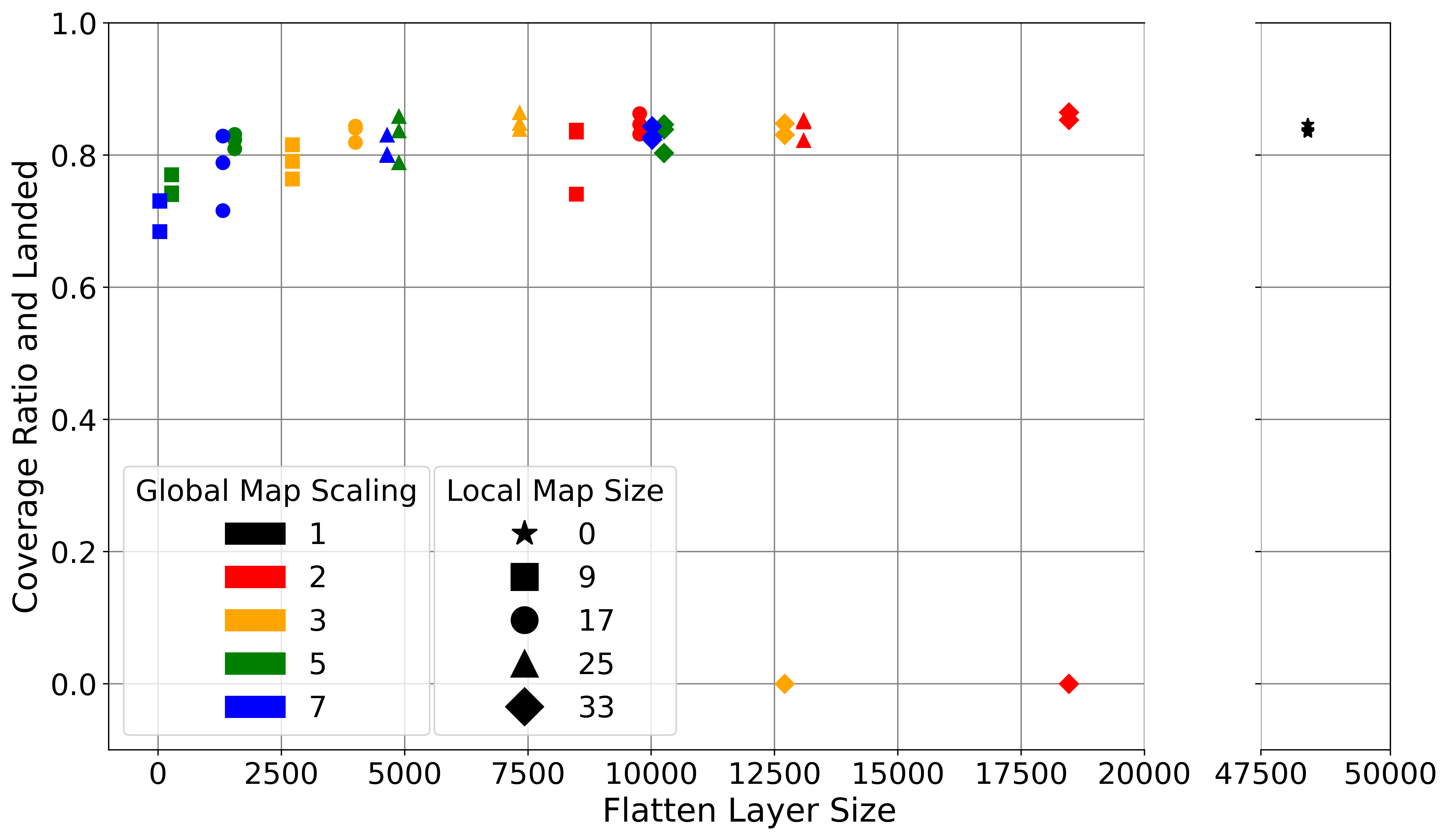
The resulting CRAL values from the Monte Carlo simulations for each agent with respect to the agent’s flatten layer size are shown in Fig. 3(a) and 3(b) for the CPP and DH problem, respectively. It can be seen that the DH problem is more sensitive to the parameters than the CPP problem. Generally, a larger flatten layer yields better performance up to a point. For both problems, it can be seen that a large flatten layer can cause the learning to get unstable, resulting in a CRAL of zero for some runs. This is caused by the agent’s failure to learn how to land. The DH agents, which are not using the global-local map approach, never learn how to land reliably and thus have a CRAL score near zero.

In both cases, the agents with $l=17$ and $g=3$ or $g=5$ show the best performance with respect to their flatten layer size, justifying the selection in Table I. Besides these two parameter combinations, it is noteworthy that the agents with $l=9$ and $g=7$ also perform well in both scenarios, despite their small flatten layer size of only 33 neurons.

References

- [1] M. Theile, H. Bayerlein, R. Nai, D. Gesbert, and M. Caccamo, “UAV coverage path planning under varying power constraints using deep reinforcement learning,” in IEEE/RSJ International Conference on Intelligent Robots and Systems (IROS), 2020.
- [2] H. Bayerlein, M. Theile, M. Caccamo, and D. Gesbert, “UAV path planning for wireless data harvesting: A deep reinforcement learning approach,” in IEEE Global Communications Conference (GLOBECOM), 2020.
- [3] Y. Zeng, Q. Wu, and R. Zhang, “Accessing from the sky: A tutorial on UAV communications for 5G and beyond,” Proceedings of the IEEE, vol. 107, no. 12, pp. 2327–2375, 2019.
- [4] R. Shakeri, M. A. Al-Garadi, A. Badawy, A. Mohamed, T. Khattab, A. K. Al-Ali, K. A. Harras, and M. Guizani, “Design challenges of multi-UAV systems in cyber-physical applications: A comprehensive survey and future directions,” IEEE Communications Surveys & Tutorials, vol. 21, no. 4, pp. 3340–3385, 2019.
- [5] T. Cabreira, L. Brisolara, and P. R Ferreira, “Survey on coverage path planning with unmanned aerial vehicles,” Drones, vol. 3, no. 1, 2019.
- [6] C. Piciarelli and G. L. Foresti, “Drone patrolling with reinforcement learning,” in Proceedings of the 13th International Conference on Distributed Smart Cameras, ACM, 2019.
- [7] K. D. Julian and M. J. Kochenderfer, “Distributed wildfire surveillance with autonomous aircraft using deep reinforcement learning,” Journal of Guidance, Control, and Dynamics, vol. 42, no. 8, pp. 1768–1778, 2019.
- [8] E. Seraj and M. Gombolay, “Coordinated control of UAVs for human-centered active sensing of wildfires,” in American Control Conference (ACC), pp. 1845–1852, IEEE, 2020.
- [9] D. Baldazo, J. Parras, and S. Zazo, “Decentralized multi-agent deep reinforcement learning in swarms of drones for flood monitoring,” in 27th European Signal Processing Conference (EUSIPCO), IEEE, 2019.
- [10] O. Esrafilian, R. Gangula, and D. Gesbert, “Learning to communicate in UAV-aided wireless networks: Map-based approaches,” IEEE Internet of Things Journal, vol. 6, no. 2, pp. 1791–1802, 2018.
- [11] C. H. Liu, Z. Dai, Y. Zhao, J. Crowcroft, D. O. Wu, and K. Leung, “Distributed and energy-efficient mobile crowdsensing with charging stations by deep reinforcement learning,” IEEE Transactions on Mobile Computing, vol. 20, no. 1, pp. 130–146, 2021.
- [12] S. Zhang and R. Zhang, “Radio map based path planning for cellular-connected UAV,” in IEEE Global Communications Conference (GLOBECOM), 2019.
- [13] J. Xie, L. R. G. Carrillo, and L. Jin, “An integrated traveling salesman and coverage path planning problem for unmanned aircraft systems,” IEEE Control Systems Letters, vol. 3, no. 1, pp. 67–72, 2019.
- [14] L. P. Kaelbling, M. L. Littman, and A. R. Cassandra, “Planning and acting in partially observable stochastic domains,” Artificial intelligence, vol. 101, no. 1-2, pp. 99–134, 1998.
- [15] H. Van Hasselt, A. Guez, and D. Silver, “Deep reinforcement learning with double Q-learning,” in Thirtieth AAAI conference on artificial intelligence, pp. 2094–2100, 2016.
- [16] S. Zhang and R. S. Sutton, “A deeper look at experience replay,” arXiv:1712.01275 [cs.LG], 2017.
- [17] R. S. Sutton, D. Precup, and S. Singh, “Between MDPs and semi-MDPs: A framework for temporal abstraction in reinforcement learning,” Artificial intelligence, vol. 112, no. 1-2, pp. 181–211, 1999.