Refining Similarity Matrices to
Cluster Attributed Networks Accurately
Abstract
As a result of the recent popularity of social networks and the increase in the number of research papers published across all fields, attributed networks—consisting of relationships between objects, such as humans and the papers, that have attributes—are becoming increasingly large. Therefore, various studies for clustering attributed networks into sub-networks are being actively conducted. When clustering attributed networks using spectral clustering, the clustering accuracy is strongly affected by the quality of the similarity matrices, which are input into spectral clustering and represent the similarities between pairs of objects. In this paper, we aim to increase the accuracy by refining the matrices before applying spectral clustering to them. We verify the practicability of our proposed method by comparing the accuracy of spectral clustering with similarity matrices before and after refining them.
Index Terms:
Attribute Networks, Clustering,Refinement of Similarity Matrices
I Introduction
In recent years, developments in information technology have led to the accumulation of a very large amount of data [1], which can no longer be managed by humans. Therefore, studies on data mining techniques to identify useful knowledge from a very large amount of data are attracting substantial attention. Among these techniques, clustering is useful for grouping data into clusters automatically, which is difficult to perform manually. Examples of data that have become unmanageable include attributed networks (ANs), each of which consists of a set of objects with attributes and relationships between the objects. Examples of ANs include social networks, which consist of relationships between humans, and citation networks, which consist of citations between documents. When we analyze a social network, the attributes of each human are his/her characteristics, such as the number of times to tweet words, and relationships between humans include follow relationships. Clustering an AN into groups, each containing humans with a high similarity to each other, has been actively studied [2][3][4].
By clustering objects in an AN into groups, we can understand some properties of the AN that cannot be discerned manually; this provides various benefits. For example, in social networks, groups are considered to be human communities; when companies use social networks to advertise their products, they can distribute advertisements to communities that may be interested in their products. Companies expect this to increase the efficiency of advertisements.
In this paper, we use spectral clustering [5] to cluster ANs. Its accuracy is strongly affected by the quality of the similarity matrices, which are necessary input for spectral clustering and represent the similarity between objects. In this paper, we aim to increase the accuracy by refining the similarity matrices before applying spectral clustering to them.
The contributions of our paper are summarized as follows:
- •
We propose a process to combine two different types of features of an AN, attributes and relationships, to derive a high-quality similarity matrix.
- •
We demonstrate that the refinement process that increases the quality of the similarity matrix is effective in the clustering of ANs using various real-world databases.
The remainder of this paper is organized as follows: In Section II, we define ANs and introduce the clustering problem for ANs. We also provide an overview of the refinement of similarity matrices. In Section III, we propose algorithms to cluster objects in an AN using the refinement process. In Section IV, we present the experimental results for real-world databases. In Section V, we discuss out proposed method and related work. In Section VI, we conclude this paper.
II Clustering of Attributed Networks using the Refinement of Similarity Matrices
II-A Clustering of Attributed Networks
First, we define ANs and introduce the clustering problem for ANs. An AN that consists of objects is a directed network , with two features and , described as follows:
-
Each has a -dimensional attribute vector whose elements represent the object’s characteristics.
-
Each element in is a direct relationship between objects and , which represents a relationship such as a follow relationship or citation.
The method proposed in this paper is applicable to any AN with attributes and direct relationships, and is not restricted to social networks and citation networks. Given an AN and the number of clusters as input, the clustering problem for ANs is to group the set of objects into disjoint subsets called clusters, each of which consists of objects that have a high similarity to each other.
We use spectral clustering to solve the clustering problem for the ANs defined above. The input for spectral clustering is a similarity matrix , whose element represents the similarity between objects and . Therefore, to perform spectral clustering, it is necessary to derive a similarity matrix . We combine the two features of an AN, and , to derive a high-quality . Specifically, the higher the value in , the greater the similarity between the attributes of the two objects and the stronger the direct relationship between them. We propose the process to derive in Section III-A. We also discuss the refinement process, which increases the quality of , in Sections II-B to II-D.
II-B Relationship Between Accuracy and Matrix Quality
To explain the refinement process, we discuss the relationships between the accuracy of spectral clustering and the quality of the similarity matrices. We consider the similarity matrix for the AN on the left-hand side of Fig. 1, with the number of clusters as input. The AN has features and , where each is a one-dimensional vector, written in orange, and each relationship is represented by a blue arrow. Additionally, the supervised clusters that we would like to detect from the AN are represented by dashed ellipses. The similarity matrix shown in the lower right of Fig. 1 is said to be of high quality because the similarity between objects that belong to the same cluster is high and the similarity between objects that belong to different clusters, and , is low. When inputting a similarity matrix into spectral clustering as input, the higher the quality of the matrix, thef greater the probability of obtaining desirable clusters. However, it is not easy to find the high-quality similarity matrix shown in the lower right of Fig. 1 because we cannot assume that supervised clusters are available. Therefore, we actually derive the high-quality similarity matrix from only the information of and , and the number of clusters ; this often results in the low-quality shown in the upper right of Fig. 1.
In this paper, we aim to refine the low-quality similarity matrix to derive a high-quality similarity matrix, without using supervised clusters. In the next subsection, we explain the refinement process.

II-C Refining the Similarity Matrices to Improve Quality
We describe the refinement process that increases the quality of the similarity matrices without the need for supervised clusters. To explain the process, we use a weighted undirected graph that corresponds to a similarity matrix . In the graph, each vertex corresponds to an object , and each weight of an edge between and corresponds to . We use to explain the refinement of the similarity matrix because and are equivalent in terms of representing ANs similarity relations.
The refinement of a similarity matrix aims to optimize to so that consists of connected components to increase the quality of . To verify that the quality of the similarity matrix whose corresponding graph consists of connected components is high, we compare the refinement process with the -nearest neighbor graph (-nng) process [5], which is one of the common process for reconstructing graphs.
The left-hand side of Fig. 2 shows a graph for an unrefined similarity matrix . If we assume that the desirable number of clusters is 2, the graph should be divided into two connected components that consist of and . In this scenario, the graph is reconstructed as using the -nng process, and as using the refinement process, as shown in Fig. 2. The main difference between and is that the edge is present in but not in . As a consequence of cutting the edge using the refinement process, the graph is reconstructed as , which has the desired two connected components.

We now explain the reason for the difference between and . The -nng method [5] leaves only edges if is one of the neighbors of with the largest weight or is one of the neighbors of with the largest weight. In Fig. 2, the edge , which has the largest weight among the edges of both and , is left in . By contrast, the refinement process reconstructs the graph as , which consists of two connected components. Therefore, it is possible to cut to reconstruct two components, and , each of whose vertices are tightly connected to each other. The refinement process increases the similarity between vertices in each cluster that we would like to detect, and reduces the similarity between vertices that belong to different clusters, compared with the -nng method. Thus, the refinement process increases the quality of the similarity matrix without using supervised clusters. In fact, the similarity matrix for derived using our refinement method is almost the same as the high-quality similarity matrix shown in the lower right of Fig. 1.

In addition to the above refinement process, our study aims to cluster ANs to achieve a high mean silhouette score. The silhouette score is one of the most popular and effective internal measures for the evaluation of clustering validity without using supervised clusters [6]. The mean silhouette score is high when the sizes of the obtained clusters are almost the same and the clusters are separate from each other. Obtaining clusters that have a high mean silhouette score prevents the refinement process from constructing connected components that are too small, that is, that consist of only a few vertices, and from obtaining them as clusters, as shown in Fig. 3. In Section III-B, we propose a process to obtain clusters that have a high mean silhouette score.
II-D Application of the Refinement Process to ANs
 politicsuk
 cora
cora
|
We expect that the refinement will increase the quality of the similarity matrices for many ANs in real-world databases. For example, Fig. 4 shows graphs for similarity matrices generated from parts of a social network called politics-uk11 1 http://mlg.ucd.ie/aggregation/index.html and a citation network called cora22 2 https://linqs.soe.ucsc.edu/data. In the figure, the similarity between objects is represented by the thickness of the edge. In Fig. 4, the vertices in each cluster, in the lower right and upper left of each of the graphs, are densely connected by thick edges. However, the vertices in different clusters are also connected by thick edges. For the graphs, the refinement process is expected to reduce the weights of the edges between clusters and increase the weights of the edges within each cluster to increase the quality of the similarity matrices.
The authors of an existing clustering method called SClump [7] proposed the above refinement process. However, SClump is applic able to networks in which “each object has only a single attribute of a discrete value but not a continuous value,” which is not true of our ANs. Therefore, SClump has the drawback that the refinement process, which was proposed in [7], cannot be applicable to the clustering of ANs. In this paper, we propose a method for clustering ANs using a refinement process by extending SClump.
III Proposed Method
In Sections II-B to II-D, we presented an overview of the refinement of similarity matrices and described SClump’s drawback: its refinement process is not applicable to the ANs considered in this paper. In this section, we propose a method for clustering ANs using a refinement process by extending SClump.
When refining a similarity matrix to , if the quality of the unrefined is high, the quality of the refined will also be high. Hence, it is very important not only to refine to but also to derive from an AN. Therefore, in Section III-A, we also propose a process for deriving . Then in Section III-B, we provide the details for an approach to refine to a high-quality .
III-A Process to Derive the Similarity Matrix
We now explain the process to derive the similarity matrix from two features—the attributes and relationships —of the AN given as input. Let the similarity matrix derived from be and the similarity matrix derived from be . We derive as the weighted sum of and with a weight vector . We explain the process to derive and as follows33 3 In the proposed process, each similarity matrix, and , is the weighted sum of several matrices, and we refine the similarity matrix , which increases the quality of , by learning the weights from the input.:
III-A1 Similarity Matrix Derived from
To derive the similarity matrix from , we calculate the similarity between and from the -th elements of and as follows:
We derive similarity matrices from the -dimensional vectors , and let the weighted sum of the similarity matrices be . The calculation in the refinement process may be unable to terminate in a reasonable time when is too large. Therefore, we reduce the number of dimensions of using principal component analysis (PCA), and update each to a low-dimensional vector in the preprocessing phase44 4 The contribution rates of PCA are used to initialize the weights to derive from ; this is described on p. 5..
III-A2 Similarity Matrix Derived from
We calculate each similarity in from the direct relationships in . When calculating similarity, we take account of the direct relationship between two objects and the transitive relationships between them; this is accomplished by considering the shortest paths (SPs) of the form .
We illustrate the necessity of transitive relationships using an AN in Fig. 5. The solid blue arrows in Fig. 5 represent the direct relationships between objects and the dotted blue arrows represent the transitive relationships, which correspond to the SPs between the objects. Specifically, we regard the SPs , whose length is less than or equal to , as the transitive relationships between and . (Hereinafter, we write “between and ” as “between .”) When is 3, as shown in Fig. 5, there is an SP between . Therefore, as shown in the dashed ellipse in Fig. 5, transitive relationships densify the cluster that we would like to detect. We expect that this densification will increase the quality of derived from the dense cluster. Furthermore, when calculating similarities, we would like to satisfy the following requirement.
- Req. 1 :
-
The shorter the SP between , the larger
the value to which we should set the similarity
between .
Requirement 1 is natural because direct relationships in an AN represent stronger connections than transitive relationships. To satisfy Req. 1, when there is an SP of length between , we set the similarity between the objects to be , as shown on the right-hand side of Fig. 5.

 (a) Similarities to satisfy Req. 2a
 (b) Similarities to satisfy Req. 2b
|
We also consider other requirements for the calculation of similarities in . In the following explanation, we use the objects in Fig. 7. In contrast to the example in Fig. 5, the number of SPs of length between and the number of SPs of length between are larger than 1. In such cases, the similarities should be calculated depending not only on the length of an SP but also the number of SPs. Moreover, when regarding objects as users, because follows fewer users than , is considered to follow closer friends than . It is unlikely that the SPs between via ’s close friends represent the same strength of connections as the SPs between . Therefore, we also wish to satisfy the following requirement.

- Req. 2 :
-
We wish to calculate similarities that increase
depending on both the length and number
of SPs.
Similarity to Satisfy Req. 2a
We define , where is the set of objects reachable from within steps. Each SP between via ’s close friend in is considered to be a stronger connection than each SP between via ’s friend in . Therefore, as shown by the red line segments in Fig. 6(a), the similarity between should be greater than the similarity between , even if both the between and the between increase by 1. The strength of the connection of each SP between depends on the cardinality of . Therefore, to satisfy Req. 2, we propose a new function to evaluate the strength of the connection:
The first and second terms in Eq. (III-A) satisfy Reqs. 1 and 2, respectively. If , ranges from to because is the proportion of and ranges from 0 to 1. When calculating the similarity between , because , the denominator is 2. By contrast, when calculating the similarity between , the denominator is 9, which decreases . Therefore, as shown by the red line segments in Fig. 6(a), Eq. (III-A) defines a larger similarity between than between , even if both between and between increase by 1.
Similarity to Satisfy Req. 2b
When all the objects in and are connected to and , respectively, the latter is considered to be a stronger connection because the number of SPs between is larger than the number between . Therefore, as shown by the blue line segments in Fig. 6(b), we want the similarity between to be greater than the similarity between when the number of SPs between and the number between reach the maximum values under the fixed . We therefore propose another function for the case where of Eq. (III-A).
| (8) |
where is constant for any two objects. Therefore, as shown by the blue line segments in Fig. 6(b), when reaches the maximum value under the fixed , the similarity between is larger than the similarity between .
Because ANs are directed networks, the similarity matrices and are not symmetric. Therefore, we update them as and to symmetrize them.
Having obtained , , and , we compute the weighted sum of these matrices with a weight vector to derive a similarity matrix . We initialize the -th element of with the contribution ratio for the -th principal component, as follows:
| (9) |
III-B Refinement Process with a Weight Adjustment
We now discuss the refinement of , which is the topic of this study. We explained that we compute the weighted sum of and to derive . The left-hand side of Fig. 8 shows an AN and the dashed ellipses represent supervised clusters. Because all the attribute values of the objects are 1, , based on the attribute values, is low quality. By contrast, because the relationships between the objects exist only in the clusters, , based on the relationships, is high quality. Because clustering is unsupervised learning, we do not know which similarity matrix is high quality before the refinement process. Therefore, there is no procedure better than computing the weighted sum of and with the weight vector initialized to , which results in a low-quality . However, if is adjusted to assign large weights to high-quality similarity matrices, we can obtain a high-quality similarity matrix by computing its weighted sum, as shown in the lower right of Fig. 8.
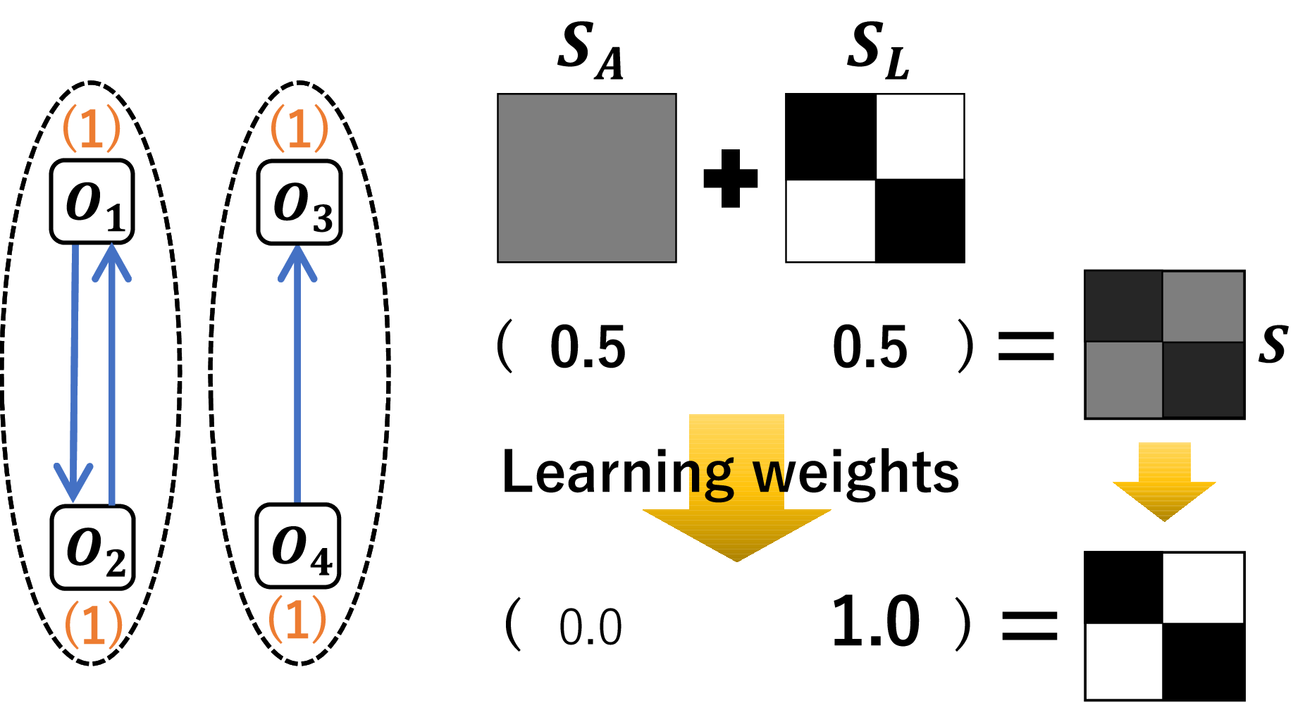
The quality of the similarity matrices is increased by adjusting as mentioned above. As mentioned in Section II-C, the similarity matrix is high quality when the graph corresponding to consists of connected components. Therefore, SClump aims to refine to , whose corresponding graph consists of connected components, by adjusting . To achieve this, SClump solves the following optimization problem, with variables , , and :
| (10) | ||||
where and each is the eigenvector corresponding to the -th smallest eigenvalue of the Laplacian matrices . Additionally, , , and are hyper parameters. The objective function in Eq. (III-B) consists of four terms. Its first term learns , which approximates derived in Eq. (9). The second and third terms are regularization terms, which prevent and from overfitting input data. The fourth term optimizes to so that its corresponding graph consists of connected components. This term achieve the refinement process as described in Section II-C. Finally, the four constraints normalize and , and make all their elements non-negative.
We solve Eq. (III-B) using an iterative update approach, called the coordinate descent approach [7]. In each iteration, two of the three variables are fixed, whereas the remaining variable is updated. When the value of the objective function in Eq. (III-B) converges, we end the iterative update approach.
Clusters with a High Mean Silhouette Score
Additionally, we also aim to obtain clusters that have a high mean silhouette score, as mentioned in Section II-C. We add a stopping criteria in the iterative update approach using the mean silhouette score [6]. This measure provides a silhouette score for each object in a cluster , taking into account both condensability and separability , as follows:
| (11) | ||||
where is the indicator, which equals 1 when is in the cluster , and 0 otherwise. Additionally, is the squared Euclidean distance between and .
The calculation of the silhouette score requires a set of clusters. Therefore, we first obtain a set of clusters by inputting into spectral clustering, where is updated times using the iterative update approach. Next, we compute the mean silhouette score based on the set of clusters . We terminate the iterative update when the reaches the local maximum that satisfies . We output the set of clusters and achieve the clustering of the AN. The pseudo code of our proposed method is summarized in Algorithm 1.
IV Evaluation Experiments
We implemented Algorithm 1 in Python55 5 https://github.com/yururyuru00/SpectralClusteringwithRefine. Table I shows the datasets containing information on social networks11footnotemark: 1 and citation networks22footnotemark: 2 that were used for our experiments.
| Dataset | #Objects | #Dimensions of | #Clusters |
|---|---|---|---|
| football11footnotemark: 1 | 248 | 11,806 | 20 |
| politics-uk11footnotemark: 1 | 419 | 19,868 | 5 |
| olympics11footnotemark: 1 | 464 | 18,455 | 28 |
| cora22footnotemark: 2 | 2,708 | 1,433 | 7 |
| citeseer22footnotemark: 2 | 3,312 | 3,703 | 6 |
Experimental Settings
On Line 1 of Algorithm 1, we derived a from attribute vectors . In the case of citation networks, we derived using cosine similarity.
When solving Eq. (III-B) and using spectral clustering, it is necessary to solve the eigenvalue problems of Laplacian matrices derived from the similarity matrices. The problems are relaxed normalized cut (NCut) and ratio cut (RCut) problems when the Laplacian matrices are normalized and unnormalized, respectively [5]. Therefore, we clustered the datasets using both normalized and unnormalized matrices.
As mentioned in Section III-B, we solve Eq. (III-B) using the iterative update approach to achieve the refinement process. A major computation performed by the iterative update approach is the updating of , which requires the solution of a quadratic programming problem for each . Although the interior point method is the common algorithm used to solve the problem, the time complexity for solving the problem for each is . However, because a fast algorithm, called simplex sparse representation, with complexity was proposed in [8], we used this algorithm. Additionally, we updated the top elements with a large similarity among , and set the others to 0, as suggested by [9]. The time complexity was thereby reduced significantly to make the algorithm easy to apply to large-scale datasets.
Parameters Settings
Metrics for Evaluating Clustering Performance
To evaluate the clustering accuracy, we used two popular metrics: normalized mutual information (NMI) and purity [10]. The values of the two metrics range from 0 to 1, and the larger the value, the higher the clustering accuracy.
IV-A Effect of Evaluating Transitive Relationships
We proposed a process that evaluates transitive relationships, in addition to direct relationships. To verify the effect of the process, we changed and fixed . When , only direct relationships were evaluated; and when , transitive relationships that corresponded to the SPs with a length up to ware also evaluated.
Table II shows the NMI when we executed Algorithm 1 on the datasets while varying . The NMI was the best for all the datasets when we set to 3. Therefore, these results demonstrate that evaluating both direct and transitive relationships was effective for clustering ANs.
| Direct | Direct + transitive | ||||
|---|---|---|---|---|---|
| Dataset | |||||
| football | 0.87 | 0.92 | 0.92 | 0.92 | 0.92 |
| cora | 0.39 | 0.41 | 0.44 | 0.43 | 0.44 |
| politics-uk | 0.89 | 0.91 | 0.93 | 0.93 | 0.93 |
| olympics | 0.92 | 0.92 | 0.93 | 0.92 | 0.92 |
| citeseer | 0.38 | 0.39 | 0.39 | 0.39 | 0.39 |
IV-B Effect of the Refinement of the Similarity Matrices in ANs
We proposed a process for clustering ANs using the refinement, to increase the clustering accuracy. To verify whether the refinement process increases the clustering accuracy, we executed Algorithm 1 on the experimental datasets.

Figure 9 shows the NMI of clustering the datasets using the refinement process. The horizontal axes show , which is the number of iterative updates of Eq. (III-B) required to achieve the refinement process. The vertical axes show the NMI when inputting updated times into spectral clustering, where and refers to in the pseudo code of Algorithm 1. Here is the unrefined , and each is a partially refined similarity matrix66 6 We use a term “partially” to indicate that that matrix is not minimized until the convergence of Eq. (III-B) and its minimization is terminated by the stopping criteria..
For all the datasets, Fig. 9 shows that the NMI of the partially refined was greater than the NMI of the unrefined . In particular, for the citeseer and cora datasets, we confirmed that the partial refinement increased the NMI. Therefore, these results demonstrate that the partial refinement, which updates until the stopping criteria was satisfied, increased the clustering accuracy for all the datasets.
Additionally, to verify whether the partial refinement actually increases the quality of the similarity matrix, Fig. 10 visualizes the unrefined (left-hand side) and the partially refined (right-hand side) for the football and cora datasets. Comparing the enlarged with the enlarged , it is clear that is almost the same as the high-quality similarity matrix shown in the lower right of Fig. 1. Each diagonal block in indicates similarities in a connected component in similar to one of the supervised clusters. We confirmed this finding in all the experimental datasets. Therefore, these results demonstrate that refinement increased the quality of the similarity matrix for all the datasets.

football
 cora
cora
We also compared our clustering method with three state-of-the-art clustering methods without using the refinement process: MVAP [11], CESNA [12], and SSB[13]. Regarding the clustering accuracy of the comparative studies, we referred to [11][13]. Table III shows the NMI and purity of the four clustering methods: MVAP, CESNA, SSB, and our method (Algorithm 1) with the refinement process. For this experiment, we executed Algorithm 1 for both normalized and unnormalized Laplacian matrices. Table III shows that our method outperformed the state-of-the-art clustering methods. The results confirm that our method using the partial refinement of the similarity matrix was very effective for high-accuracy clustering ANs for the olympics, cora, and citeseer datasets.
| No refinement | Refinement (Algorithm 1) | |||||
|---|---|---|---|---|---|---|
| Dataset | Metric | MVAP | CESNA | SSB | Normalized | Unnormalized |
| olympics | NMI | Not listed | 0.48 | 0.50 | 0.90 | 0.91 |
| Purity | Not listed | 0.36 | 0.36 | 0.93 | 0.94 | |
| cora | NMI | 0.26 | 0.12 | 0.20 | 0.44 | 0.38 |
| Purity | 0.27 | 0.30 | 0.38 | 0.60 | 0.54 | |
| citeseer | NMI | 0.21 | 0.18 | 0.23 | 0.31 | 0.39 |
| Purity | 0.26 | 0.19 | 0.40 | 0.51 | 0.61 | |
IV-C Refinement Details
As shown in Fig. 9, we confirm that the partial refinement, which updated until satisfying the stopping criteria, increased the NMI. By contrast, we found that the complete refinement of the similarity matrix, which means minimizing Eq. (III-B) without the stopping criteria of the mean silhouette score, reduced the NMI. To verify this finding, the blue lines in Fig. 11 show the mean silhouette scores. The horizontal axes show , which is the number of iterative updates of the refinement process, where , and refers to in the pseudo code of Algorithm 1. The blue lines show the mean silhouette scores based on the predictive clusters , which were obtained at each iteration.
For all the datasets, Fig. 11 shows that the mean silhouette scores reached the maximum at , and thereafter reduced when became larger than . The effect of the refinement was to optimize the similarity matrix so that consisted of connected components. Additionally, the mean silhouette score was high when the sizes of connected components obtained as clusters were almost the same and separate from each other. Therefore, the high silhouette score at means that the partial refinement separated connected components whose cluster sizes were almost the same. Moreover, for all the datasets in Fig. 11, there were strong correlations between the mean silhouette scores (blue lines) and NMIs (orange lines). Therefore, we confirmed that the unevenly sized and non-separated connected components generated by the complete refinement beyond the stopping criteria led to a reduction of the clustering accuracy.

V Discussion of Related Work
In this section, we discuss the novelty of our study when compared with SClump [7], which is the basis of our study. As mentioned in Section II-D, SClump is applicable to heterogeneous information networks (HINs) in which “each object has only a single attribute of a discrete value,” which is not true of our ANs in which “each object has multiple attributes of continuous values.” We explain why SClump cannot be applied to ANs.
As mentioned in Section III-B, the refinement of the similarity matrix requires multiple similarity matrices summarized in . To compute each similarity of the matrices, SClump uses a meta-path, which is a measure for calculating similarity based on a single attribute that each object has and relationships between objects in HINs. Therefore, for the clustering of ANs with the refinement process, it is necessary to propose a new measure based on multiple attributes of each object and relationships between objects in ANs. We proposed new measures in Section III-A, and these measures enabled the refinement to be applicable to not only HINs but also ANs.
Additionally, regarding the refinement process, the authors of SClump proposed the complete refinement which updates until Eq. (III-B) converges. By contrast, we proposed the partial refinement, in addition to the traditional complete refinement, by adding a stopping criteria in Eq. (III-B). The evaluation experiments in Section IV-B show that the partial refinement is effective in the clustering of ANs. Furthermore, in Section IV-C, we verified that the complete refinement reduced the clustering accuracy of ANs.
VI Conclusion
We proposed a method for high-accuracy clustering of ANs. The method contains the process to evaluate both direct and transitive relationships between objects to derive a high-quality similarity matrix. In addition, it contains another process to apply refinement to ANs to increases the clustering accuracy.
Evaluation experiments showed that the first process is effective for clustering ANs. We also confirmed that partial refinement, rather than complete refinement proposed in [7], increases the clustering accuracy of ANs. We showed that our proposed method outperforms state-of-the-art clustering methods without the refinement. From the above, we confirmed that our proposed method is effective for the high-accuracy clustering of ANs.
References
- [1] Khan N, Yaqoob I, Hashem IA, Inayat Z, Ali M, Kamaleldin W, Alam M, Shiraz M, Gani A. Big data: survey, technologies, opportunities, and challenges. The scientific world journal. 2014;2014.
- [2] Bothorel C, Cruz JD, Magnani M, Micenkova B. Clustering attributed graphs: models, measures and methods. Network Science. 2015 Sep;3(3):408-44.
- [3] Xu Z, Ke Y, Wang Y, Cheng H, Cheng J. A model-based approach to attributed graph clustering. InProceedings of the 2012 ACM SIGMOD international conference on management of data 2012 May 20 (pp. 505-516).
- [4] Xu Z, Ke Y, Wang Y, Cheng H, Cheng J. GBAGC: A general bayesian framework for attributed graph clustering. ACM Transactions on Knowledge Discovery from Data (TKDD). 2014 Aug 25;9(1):1-43.
- [5] Von Luxburg U. A tutorial on spectral clustering. Statistics and computing. 2007 Dec 1;17(4):395-416.
- [6] Wang F, Franco-Penya HH, Kelleher JD, Pugh J, Ross R. An analysis of the application of simplified silhouette to the evaluation of k-means clustering validity. InInternational Conference on Machine Learning and Data Mining in Pattern Recognition 2017 Jul 15 (pp. 291-305). Springer, Cham.
- [7] Li X, Kao B, Ren Z, Yin D. Spectral clustering in heterogeneous information networks. InProceedings of the AAAI Conference on Artificial Intelligence 2019 Jul 17 (Vol. 33, pp. 4221-4228).
- [8] Huang J, Nie F, Huang H. A new simplex sparse learning model to measure data similarity for clustering. InTwenty-Fourth International Joint Conference on Artificial Intelligence 2015 Jun 27.
- [9] Nie F, Wang X, Jordan MI, Huang H. The constrained laplacian rank algorithm for graph-based clustering. InThirtieth AAAI Conference on Artificial Intelligence 2016 Mar 2.
- [10] Rezaei M, Fränti P. Set matching measures for external cluster validity. IEEE Transactions on Knowledge and Data Engineering. 2016 Apr 7;28(8):2173-86.
- [11] Wang CD, Lai JH, Philip SY. Multi-view clustering based on belief propagation. IEEE Transactions on Knowledge and Data Engineering. 2015 Nov 25;28(4):1007-21.
- [12] Yang J, McAuley J, Leskovec J. Community detection in networks with node attributes. In2013 IEEE 13th International Conference on Data Mining 2013 Dec 7 (pp. 1151-1156). IEEE.
- [13] Chen H, Yu Z, Yang Q, Shao J. Attributed Graph Clustering with Subspace Stochastic Block Model. Information Sciences. 2020 May 21.