Renormalon Effects in Quasi Parton Distributions
Abstract
We investigate the renormalon ambiguity from bubble-chain diagrams in the isovector unpolarized quasi- parton distribution function (PDF) of a hadron. We confirm the assertion by Braun, Vladimirov and Zhang Braun et al. 2019 that the leading IR renormalon ambiguity is an effect, with the parton momentum fraction and the hadron momentum, together with a new contribution such that the quark number is conserved. This implies the convergence of the perturbative matching kernel between a quasi-PDF and a PDF would eventually fail for small . However, in both the R-scheme designed to cancel the leading IR renormalon and the typically used RI/MOM scheme in lattice QCD for the same quasi-PDF, we find good convergence in the kernel based on three-loop bubble-chain diagram analyses. These results are encouraging for the quasi-PDF program. However, firm conclusions can only be drawn after the complete higher loop QCD calculations are carried out.
I Introduction
Large momentum effective theory (LaMET) enables computations of parton distributions of hadrons on a Euclidean lattice. LaMET relates equal-time spatial correlators (whose Fourier transforms are called quasi-distributions) to lightcone distributions in the infinite hadron momentum limit Ji 2013; Ji 2014. For large but finite momenta accessible on a realistic lattice, LaMET relates quasi-distributions to physical ones through a factorization theorem, which involves a matching coefficient and power corrections that are suppressed by the hadron momentum. The proof of factorization was developed in Refs. Ma and Qiu 2018a; Izubuchi et al. 2018; Liu et al. 2019.
Since LaMET was proposed, a lot of progress has been made in the theoretical understanding of the formalism Xiong et al. 2014; Ji and Zhang 2015; Ji et al. 2015a; Xiong and Zhang 2015; Ji et al. 2017; Monahan 2018; Stewart and Zhao 2018; Constantinou and Panagopoulos 2017; Green et al. 2018; Izubuchi et al. 2018; Xiong et al. 2017; Wang et al. 2018; Wang and Zhao 2018; Xu et al. 2018a; Chen et al. 2016; Zhang et al. 2017; Ishikawa et al. 2016; Chen et al. 2017a; Ji et al. 2018a; Ishikawa et al. 2017; Chen et al. 2018a; Alexandrou et al. 2017a; Constantinou and Panagopoulos 2017; Green et al. 2018; Chen et al. 2018a; Chen et al. 2017b; Lin et al. 2018a; Chen et al. 2017c; Li 2016; Monahan and Orginos 2017; Radyushkin 2017a; Rossi and Testa 2017; Carlson and Freid 2017; Ji et al. 2017; Briceño et al. 2018; Hobbs 2018; Jia et al. 2017; Xu et al. 2018b; Jia et al. 2018; Spanoudes and Panagopoulos 2018; Rossi and Testa 2018; Liu et al. 2018a; Ji et al. 2019a; Bhattacharya et al. 2019; Radyushkin 2019a; Zhang et al. 2019a; Li et al. 2019; Braun et al. 2019; Detmold et al. 2019; Sufian et al. 2020; Shugert et al. 2020; Green et al. 2020; Braun et al. 2020; Lin 2020a; Bhat et al. 2020; Chen et al. 2020a; Ji 2020a; Chen et al. 2020b; Chen et al. 2020c; Alexandrou et al. 2020a; Fan et al. 2020a; Ji et al. 2020a. The method has been applied in lattice calculations of parton distribution functions (PDF’s) for the nucleon Lin et al. 2015; Chen et al. 2016; Lin et al. 2018a; Alexandrou et al. 2015; Alexandrou et al. 2017b; Alexandrou et al. 2017a; Chen et al. 2018a; Lin et al. 2018b; Alexandrou et al. 2018a; Chen et al. 2018b; Alexandrou et al. 2018b; Lin et al. 2018c; Fan et al. 2018; Liu et al. 2018b; Wang et al. 2019; Lin and Zhang 2019; Liu 2020; Lin and Zhang 2019; Zhang et al. 2020a, Chen et al. 2018c; Izubuchi et al. 2019; Gao et al. 2020 and Lin et al. 2020 mesons. Despite limited volumes and relatively coarse lattice spacings, the state-of-the-art nucleon isovector quark PDF’s, determined from lattice data at the physical point, have shown reasonable agreement Lin et al. 2018b; Alexandrou et al. 2018a with phenomenological results extracted from the experimental data. Encouraged by this success, LaMET has also been applied to Chai et al. 2020 and twist-three PDF’s Bhattacharya et al. 2020a; Bhattacharya et al. 2020b; Bhattacharya et al. 2020c, as well as gluon Fan et al. 2020b, strange and charm distributions Zhang et al. 2020b. It was also applied to meson distribution amplitudes Zhang et al. 2017; Zhang et al. 2019b; Zhang et al. 2020c and generalized parton distributions (GPD’s) Chen et al. 2019; Alexandrou et al. 2020b; Lin 2020b; Alexandrou et al. 2019. More recently, attempts have been made to generalize LaMET to transverse momentum dependent (TMD) PDF’s Ji et al. 2015b; Ji et al. 2018b; Ebert et al. 2019a; Ebert et al. 2019b; Ebert et al. 2020a; Ji et al. 2020b; Ji et al. 2019b; Ebert et al. 2020b to calculate the nonperturbative Collins-Soper evolution kernel Ebert et al. 2019a; Shanahan et al. 2020a; Shanahan et al. 2020b and soft functions Zhang et al. 2020d on the lattice. LaMET also brought renewed interests in earlier approaches Liu and Dong 1994; Detmold and Lin 2006; Braun and Müller 2008; Bali et al. 2018a; Bali et al. 2018b; Detmold et al. 2018; Liang et al. 2020 and inspired new ones Ma and Qiu 2018b; Ma and Qiu 2015; Chambers et al. 2017; Radyushkin 2017b; Orginos et al. 2017; Radyushkin 2018a; Radyushkin 2018b; Zhang et al. 2018; Karpie et al. 2018; Joó et al. 2019a; Radyushkin 2019b; Joó et al. 2019b; Balitsky et al. 2020; Radyushkin 2020; Joó et al. 2020; Can et al. 2020. For recent reviews, see, e.g., Refs. Lin et al. 2018d; Cichy and Constantinou 2019; Zhao 2020; Ji et al. 2020c; Ji 2020b.
The quark PDF in a proton is related to a lightcone correlator
| (1) |
where the proton momentum is alone the -direction, , and is the lightcone coordinates. is the parton momentum fractions relative to the proton. is a gauge field and is a quark field. The expression in Eq.(1) is boost invariant alone the -direction. The corresponding quasi-PDF is related to an equal time correlator Ji 2013; Ji 2014
| (2) |
LaMET relates the flavor non-singlet quark quasi-PDF and PDF of a hadron through the factorization theorem
| (3) |
where and are renormalization parameters and PDF is defined in the infinite momentum frame with Ji 2013; Ji 2014. The (quasi-)PDF for negative momentum fraction corresponds to the (quasi-)PDF of the anti-particle. In particular, with denoting an antiquark PDF.
Let us first discuss the case that both the quasi-PDF and PDF are defined in cut-off schemes with UV cut-off and , respectively. The factorization theorem is based on a large momentum expansion in powers of . The correction has a similar convolutional structure to the first term: . The scales follow the hierarchy , such that the short distance (compared with ) physics is encoded in the matching kernels (or Wilson coefficients) and while the long distance physics is encoded in the matrix elements and with of twist-2 and of twist-. In this series, the long and short distance physics are strictly separated by the scale .
However, the PDF’s extracted from experimental data are typically defined in the modified minimal subtraction () scheme. This is because the PDF’s convolute with Wilson coefficients to form observables in high energy experiments, and it is technically much easier to compute the Wilson coefficients to higher loops in than a hard cut-off scheme. However, there is no strict separation between long and short distance physics in the scheme. This means the Wilson coefficients could still contain non-perturbative physics called renormalons Gross and Neveu 1974; Lautrup 1977; ’t Hooft 1979 to cause slow convergence in their perturbative expansions.
Mathematically, the renormalon effect could arise when Borel transform is applied to improve the convergence of a perturbation series. Then an inverse Borel transform is applied after the Borel series is summed. However, sometimes the bad convergence of the series can not be tamed by the Borel transform but appears as ambiguities in the inverse Borel transform. When is defined in the scheme with renormalization scale and the quasi-PDF is defined in the regularization-independent momentum subtraction (RI/MOM) scheme Stewart and Zhao 2018 with scale , Eq.(3) can be rewritten as
| (4) |
Since scale separation is not complete in and RI/MOM, low energy non-perturbative physics could still exist in , which slows down the convergence of the perturbative computation of . It can be shown that by resumming a class of bubble-chain diagrams in with the help of Borel transform, there are ambiguities in the inverse Borel transform which behave like non-perturbative functions with .
Since these ambiguities are associated with different choices of the integration paths in the inverse Borel transform, they are not physical. They should be cancelled by the terms. Therefore all the ’s need to be defined consistently. An independent determination of a higher twist is not meaningful unless the treatment of renormalon ambiguity in the lower twist is specified. Furthermore, one can estimate the size of by the size of the renormalon ambiguity in . It was through this analysis that Braun, Vladimirov and Zhang asserted that the leading IR renormalon ambiguity was an effect Braun et al. 2019, which was larger than the previous estimation based on dimensional analysis by a factor . Therefore, this result has a big impact to the LaMET program. This motivates us to re-investigate the renormalon problem in quasi-PDF.
II Renormalon Ambiguity in Quasi-PDF’s
In this section we first briefly review the Borel transform and the possible ambiguity in its inverse transformation. After the discoveries of renormalons Gross and Neveu 1974; Lautrup 1977; ’t Hooft 1979 and further conceptual developments ’t Hooft 1979; Parisi 1978; Parisi 1979; David 1984; David 1986; Mueller 1985, higher order behaviors of perturbation series in the context of renormalon ambiguities became relevant phenomenolically Brown and Yaffe 1992; Zakharov 1992; Mueller 1992. (See, e.g., Ref.Beneke 1999 for a review). We will compute the renormalon ambiguity caused by the bubble-chain diagrams to the quasi-PDF. We will compute the Feynman diagrams in momentum space then compare our result with the coordinate space computation obtained in Ref. Braun et al. 2019.
We start with writing the matching kernel of Eq.(4) as a series expansion in the strong coupling constant ,
| (5) |
where we have only kept the dependence and dropped the other quantities for brevity. In the scheme with renormalization scale ,
| (6) |
where , being the number of colors, and being the number of quark flavors, and is the strong interaction scale. The series is more convergent after the Borel transform
| (7) |
After the Borel series is summed, one can perform an inverse Borel transform back to the original series:
| (8) |
If the integrant has poles on the real positive axis, then the above integral will depend on the path of integration on the complex plane. This uncertainty is called renormalon ambiguity. In an operator product expansion with the scheme, the renormalon ambiguities in the lower order Wilson coefficients will be cancelled by the higher order matrix elements.
The existence of the renormalon ambiguity is usually demonstrated in the large limit with powers of counted as and summed to all orders. Then renormalon ambiguity can arise in the expansion of these diagrams. However, it is also well known that QCD is not asymptotically free in the large limit. Therefore, even though the finite contribution can be formally included by an expansion, this expansion is not convergent in QCD. However, if we take the QCD function as a reference, it is probably reasonable to expect that subleading corrections are about the same magnitude as the leading order. If this expectation turns out to be true, then the large analysis will still be useful. Therefore, we focus on the leading diagrams in the large limit to study the renormalon ambiguity in the matching formula between a quasi-PDF and a PDF defined in Eq.(4).
When is counted as , the bubble chain diagrams that dress the gluon propagator in the second row of Fig. 1 are all . The gray bubble, which is the gluon vacuum polarization, becomes a fermion loop diagram in the large limit. We will add the gluon loop contribution to the gluon vacuum polarization as an correction as performed in Beneke 1999; Braun et al. 2019. This is formally a subleading effect in the expansion, but numerically important in QCD—it changes the sign of the QCD beta function from positive to negative. Therefore, the grey bubble in Fig. 1 is the gluon vacuum polarization at one loop Grozin 2005; Beneke 1999; Lautrup 1977; Gross and Neveu 1974
| (9) |
where is the gluon momentum and the 5/3 factor is associated with the scheme. Summing the bubble-chains yields a factor modifying the gluon propagator:
| (10) |
which has a form of an inverse Borel transform with the Borel series . We will rewrite it as times a factor which is moved to Eq.(12). Therefore, to compute the diagrams of Fig.1, one just have to replace the gluon propagator by a dressed one to obtain the Borel series:

| (11) |
where Eq.(6) is used.
Below we list the unpolarized isovector PDF and quasi-PDF results of these diagrams. The Borel series of the bubble-chain diagrams in Fig.1 yields the quark-level quasi-PDF (defined similarly to Eq. (2) but with the external hadronic state replaced by a single quark state of momentum ):
| (12) |
where is the off-shellness parameter for external quarks. is the quark spinor factor . with the number of colors. The plus-function
| (13) |
We have computed up to an integral of the Feynman parameter ,
| (14) | ||||
It is easy to see that for positive and finite , if is different from or and is different from or , then the integrant in the above integral will not diverge. For , the integration diverges when is bigger than a certain value. To see the poles in , one performs the integration by assuming is small enough such that the integration is finite. Then an analytic continuation of is performed to look for poles in . After this exercise, no additional pole at is found. The pole is corresponding to the UV divergence of the Wilson line self-energy diagram, which can be subtracted away by the renormalization procedure, such as the RI/MOM scheme used in this work. Therefore we do not consider it further here. The pole is not on the path of integration of the inverse Borel transform and hence does not cause any ambiguity.
Setting the external quark on-shell (), Eq.(14) for the unphysical region ( and ) becomes
| (15) | ||||
where is a hypergeometric function. There is no IR renormalon in this region, except the contribution near which yields the delta function in Eq.(20). The UV renormalon at can be subtracted away by the renormalization procedure discussed above and will not be discussed further.
In the physical region , IR renormalons exist. They correspond to single poles of at all positive integer values of :
| (16) | ||||
The leading IR renormalon ambiguity in the inverse Borel transform of is proportional to the residue of the single pole at . Eqs.(15) and (16) yield
| (17) |
When , the term is zero for but undetermined for . It is in fact a delta function since
| (18) |
This is consistent with the result of Ref. Schwartz 2014:
| (19) |
Eq. (17) yields
| (20) |
and the leading IR renormalon ambiguity in the inverse Borel transform of is thus given by
| (21) |
We stress that the IR renormalon is associated with the IR divergence generated when all the particles in the loop become on-shell simultaneously. This is purely an IR effect. Therefore, there is no dependence on the UV regulator in Eq. (21).

After discussing the quasi-PDF, we now turn to the PDF. The quark-level PDF is defined similarly to Eq. (1) but with the external hadronic state replaced by a single quark state of momentum . The Borel series of the bubble-chain diagrams in Fig.1 for quark-level PDF can be obtained by taking to infinity before integrating the spacial loop momenta in other directions. The result is
| (22) |
where
| (23) | ||||
and where the dimensional regularization parameter is kept because we want to perform a expansion later and this helps to keep the factor regulated. The quark-level PDF does not have any IR renormalon ambiguity as there is no pole in the Borel series in the positive real axis. This result is expected, since the PDF is corresponding to quasi-PDF in the limit and the leading IR renormalon, which is is proportional to as shown in Eq. (21), vanishes in this limit.
We can now study how this leading renormalon ambiguity affects the quasi-PDF of a hadron, , through the matching kernel of Eq.(4). The kernel can be converted from Eq.(21) by replacing the quark momentum with , being the hadron momentum, and replacing with , such that
| (24) | ||||
where the integration limit in the second line can be replaced by since vanishes outside of and we have expanded around before acting it with in the fourth line.
The plus-function in Eq. (24) ensures quark number conservation, such that . One can show the first two terms in the last line of Eq. (24) cancel after integrating over , and the last two terms are proportional to , which yields vanishing boundary terms after integrating over . Our Eq. (24) is the same as the coordinate space calculation in Ref. Braun et al. 2019.11 1 Except our prefactor of is rather than as in Ref. Braun et al. 2019. But if one starts from the first line of Eq. (61) of Ref. Braun et al. 2019, then the prefactor will be . So this should be a typo of Ref. Braun et al. 2019.
In Fig.2, the leading renormalon ambiguity in the proton isovector quasi-PDF, is shown, together with the corresponding PDF, , and the one-loop quasi-PDF , all in the scheme. Numerically, is a significant effect. Its size is bigger than for almost the entire region of . In the computation, we have used from the proton isovector (i.e. the quark combination) PDF extracted by the CTEQ-JLab collaboration (CJ12) Owens et al. 2013. , which is also shown in Fig. 3, is computed with convoluted with the one-loop matching kernel. The renormalon ambiguity of is computed with Eq. (24) with GeV and GeV. The areas under and are both one, the isovector charge, while the area under is zero, with a large negative contribution near . This is the result of fermion number conservation.
The singular behavior near requires the introduction of an IR regulator
| (25) |
When is taken at the end of the calculation, the contribution for becomes with a divergent prefactor. This illusive contribution could be easily overlooked in a numerical analysis. But it is critical for the demonstration of quark number conservation, which is a property of the bubble-chain diagrams that we considered.
Both and have support in . When or ,
| (26) |
which is consistent with Ref. Braun et al. 2019. The quasi-PDF , however, has support for all values of . Hence has no enhancement compared to . Therefore,
| (27) |
Since the renormalon ambiguity discussed above should be cancelled by power corrections, one can rewrite Eq.(4) as
| (28) |
where the first power correction has no factor and the second power correction has a divergent prefactor.
III Removing the leading renormalon ambiguity
Although the bubble-chain diagrams employed in the analysis above might not be numerically the dominant contribution in QCD, we still expect that they will generate all structures of the renormalon ambiguity Brown and Yaffe 1992. Hence Eq.(28) should be quite robust and is expected to be free from the shortcoming of the bubble-chain diagram analysis.
The R-scheme proposed in Ref. Hoang et al. 2010 is designed to remove the leading renormalon ambiguity in a general operator product expansion. In our case, the leading renormalon ambiguity in the matching factor and the leading power corrections are both proportional to in Eq.(28). These terms can be removed in the following combination:
| (29) | ||||
The remaining power corrections can in principle be removed in a similar way as well. The logarithmic term comes from the correction in the kernel which can be recasted to anomalous dimension such that the leading renormalon ambiguity in scales as . This power can be removed by replacing in the square brackets. Now the remaining power correction is . So the procedure can be applied again to remove this power correction. However, the computation of the anomalous dimensions beyond the bubble-chain diagrams could be a challenge in removing subleading renormalon ambiguities with this method.
Ref. Braun et al. 2019 also proposed a method to remove the leading renormalon ambiguity by replacing the of Eq.(2) with a combination of and . The idea is that PDF can be extracted using either or matrix element. However, the leading renormalon ambiguity contributes differently in the two cases. By choosing a specific combination of the and matrix elements, the leading renormalon ambiguity is largely canceled. However, knowing what combination to use is difficult beyond the bubble-chain approximation. Also, this proposal has another technical issue. On a lattice, the matrix element using will mix with another operator of the same dimension that needs to be removed, while the matrix element using does not have this problem. Therefore, typically is used in lattice computations. However, for the purpose of this work, both of the choices are equivalent since the analysis is performed in the continuum.
IV Bubble-Chain Contributions in Fixed Order Perturbations
In the previous section, we have seen that the leading IR renormalon ambiguity of Eq.(24) yields power corrections of Eq.(28) with singular prefactors after summing the bubble-chain diagrams to all orders in . These terms are canceled in the R-scheme by design in Eq.(29). It is natural to ask, if the cancellation works when the series is summed to all orders in , can the cancellation also happen if the series is truncated to a fixed order? It seems the answer should be yes if the cancelation works for the infinite series and for different values of (within the radius of convergence), then the cancelation ought to happen at each order in as well.
To answer this question, we need multi-loop corrections to the PDF and quasi-PDF. However, complete results beyond one-loop does not exist yet because of their technical difficulty. Therefore, we resort to large expansion again and only include the bubble-chain diagrams. As we will see in Fig. 4(b), the R-scheme could indeed introduce large cancellation of the bubble-chain diagrams at each order in . This is consistent with what Ref. Hoang et al. 2010 advocated and demonstrated that R-scheme indeed improved the convergences of QCD perturbation.
Now we show how to extract the fixed order result from the bubble summed result. The bubble-chain contribution to the -th loop quasi-PDF in the scheme can be extracted by expanding the Borel series of Eq.(12) in powers of :
| (30) | ||||
where
| (31) |
The bubble-chain contribution to the -th loop PDF in the scheme is
| (32) | ||||
where
| (33) |
The results for , , together with the to matching kernel
| (34) |
for are listed in the Appendix.
These matching kernels are free from IR divergence from diagram-by-diagram cancellations. Note that we should have also included the convolution term in the kernel and the term in the kernel were we to include all the -loop diagrams rather than just the bubble-chain diagrams. But here we only investigate how the bubble-chain diagrams which could give rise to the renormalon ambiguities converge at higher loops.
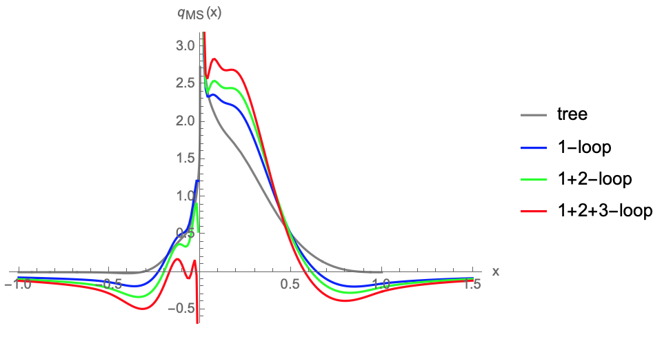


To check the effect of the bubble-chain contribution at the -loop, we convolute the CJ12 proton isovector PDF Owens et al. 2013 with of Eq.(34) to obtain the corresponding isovector quasi-PDF of the proton at -loop in the scheme. The result up to 3-loops is shown in Fig.3. We see that the two-loop contribution is smaller than one-loop but about the same size as the three-loop. Therefore the convergence is already slow at three-loop for the quasi-PDF. However, as shown in Fig. 4, the convergence is much better when we use the R-scheme of Eq.(29), especially when a larger is used. The need to use a large can be understood because for a fixed order expansion, the kernel only has powers of dependence but not dependence. Hence when we take , R-scheme reduces to the usual scheme shown in Fig.3 and has slow convergence. Therefore, larger tends to yield larger cancellation of the bubble-chain diagrams.
After establishing the power of R-scheme in removing the bubble-chain diagram contributions in 2- and 3-loop diagrams, we turn to the RI/MOM scheme which is typically used in lattice QCD and see how bubble-chain diagrams contribute in this scheme. In RI/MOM, all the loop corrections to the matrix element of a single quark state with momentum are subtracted non-perturbatively at an off-shell kinematics and . In momentum space, this amounts to the subtraction Stewart and Zhao 2018
| (35) |
with . The RI/MOM renormalized quasi-PDF is UV finite, so it does not matter what UV regulator is used to compute of Eq.(35). The UV regulator will be removed at the end to obtain . We will just replace in Eq.(34) by to get the to RI/MOM matching kernel. It is worth commenting that all the IR renormalon ambiguity comes from the first term in Eq.(35). The second term, the counterterm, takes the external quark off-shell, hence the Feynman diagrams do not experience IR divergence using the gluon propagator of Eq. (11). Therefore, the subtraction in the RI/MOM scheme does not add additional renormalon ambiguity.
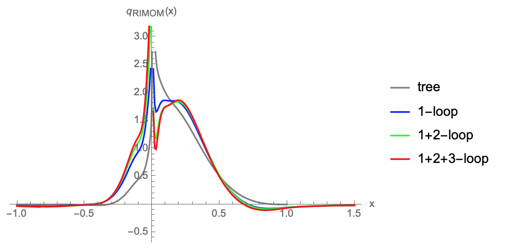
The effect of applying the RI/MOM renormalization to the proton isovector quasi-PDF up to three-loop bubble-chain diagrams is shown in Fig.5. Convergence is seen for the whole range of —the possible slow convergence due to the renormalon effect does not appear up to three-loops in the RI/MOM scheme. Of course, this result is not conclusive for QCD due to the non-convergence problem of the expansion mentioned above. However, the convergence pattern in the large world is still interesting on its own. It gives some hope that QCD might have a similar convergence pattern. But one can only know after carrying out the complete higher loop calculations.
Finally, we comment on whether we can take advantage of choosing the BLM scales Brodsky et al. 1983 to improve the convergence of the series expansion. The BLM approach is based on the observation that
| (36) |
Hence by choosing a different renormalization scale for each order in the expansion, one can completely remove all the dependence in the expansion to speed up the convergence. Interestingly, the dependence is exactly what the bubble-chain diagrams yield (see e.g. Eq.(30)). Hence the BLM approach can cancel the renormalon ambiguity from the bubble-chain diagrams to improve the convergence. However, unlike the factor of Eq.(36) is a constant, the prefactors of our matching kernel depend on the momentum fraction. It is not clear how to absorb them into renormalization scales. Even if we proceed by demanding the bubble-chain diagrams be canceled only for a specific momentum fraction, we still need to benchmark the convergence of this approach with the complete multi-loop results which are not yet available. Therefore, we do not pursuit this program here in this work.
V Conclusion
We have investigated the renormalon ambiguity in the flavor non-singlet quasi-PDF of a hadron. We follow the usual practice to study the diagrams in the large (the number of fermion flavors) limit with powers of summed to all orders Beneke 1999. Although QCD is not asymptotically free in this limit, the qualitative features of the renormalon ambiguity are expected to remain in QCD Brown and Yaffe 1992. Also, taking the function of QCD as a reference, it might be possible that the higher order corrections of our calculation are about the same magnitude as the leading order. In that case, our large analysis could still be useful although conclusive results can only be drawn with explicit full QCD calculations.
The bubble-chain diagrams were computed in momentum space and the result agreed with the coordinate space computation of Ref. Braun et al. 2019 up to one possible typo in a prefactor. We confirmed the assertion of Ref. Braun et al. 2019 that the leading IR renormalon ambiguity from bubble-chain diagrams was an effect on the quasi-PDF. In addition, we have also found an term with a divergent prefactor such that quark number conservation is not broken. This ambiguity is supposed to be cancelled by power corrections associated with higher-twist contributions. Hence, if the power corrections were not included in the analysis, then the error was , which is quite significant at small enough , rather than from dimensional analysis.
To remove this leading IR renormalon ambiguity, we have investigated the proposed R-scheme Hoang et al. 2010, which is designed to cancel all the contributions. This cancelation does not rely on the bubble-chain approximation. It is applicable in QCD. Furthermore, since the R-scheme cancel the renormalon ambiguity non-perturbatively for different values of , it is possible that the cancellation also happens at each order in to improve the convergence of QCD perturbation Hoang et al. 2010. Because the full multi-loop results in QCD are not available, we use the bubble-chain diagrams to demonstrate this up to three-loops in Fig. 4(b).
After establishing the power of R-scheme in removing the bubble-chain diagram contributions, we turn to the RI/MOM scheme which is typically used in lattice QCD and see how bubble-chain diagrams contribute to the proton isovector quasi-PDF in Fig.5. Convergence is seen for the whole range of —the possible slow convergence due to the renormalon effect does not appear up to three-loops in the RI/MOM scheme. Of course, this result is not conclusive for QCD due to the non-convergence problem of the expansion mentioned above. But it gives some hope that QCD might have a similar convergence pattern. The final result can only be known after carrying out the complete higher loop calculations.
Acknowledgments
We thank Iain Stewart for early involvement of this project and Jian-Hui Zhang for useful discussions. This work is partly supported by the Ministry of Science and Technology, Taiwan, under Grant No. 108-2112-M-002-003-MY3 and the Kenda Foundation.
Appendix A Loop Expansion of the bubble-chain Diagrams
In this Appendix, we show the -th loop correction to the lightcone PDF and quasi-PDF for a single quark state. We only show the result in the scheme. The non-perturbative renormalization of the quasi-PDF in the RI/MOM scheme can be constructed using Eq.(35).
A.1 One-loop result
The 1-loop correction to quasi-PDF of a single quark state is
| (37) |
where
| (38) | ||||
Taking the limit and isolating the logarithmic IR divergence, we have
| (39) |
The one-loop correction to the lightcone PDF of a single quark state is non-vanishing only when , and
| (40) |
where
| (41) |
The matching kernel for and , both in the scheme, is
| (42) | ||||
The IR divergence is cancelled between the quasi-PDF and PDF in the matching kernel as we expect that the kernel only compensates the UV difference between the quasi-PDF and PDF.
The kernel has the asymptotic behavior
| (43) |
with . This leading contribution is cancelled in the RI/MOM to scheme matching which yields better convergence numerically Stewart and Zhao 2018.
A.2 Two-loop result
The two-loop correction to quasi-PDF of a single quark state can be written as
| (44) |
The first term comes from the sub-divergence of the gluon vacuum polarization bubble. Taking the limit and isolating the logarithmic IR divergence, we have
| (45) |
The two-loop lightcone PDF is only non-vanishing for
| (46) |
where
| (47) |
To this end we will define the matching kernel as
| (48) | ||||
which is again free from IR divergence as in the one-loop case. The IR divergence cancellation works diagram by diagram between the quasi-PDF and the PDF. However, we should have also included the convolution term in the kernel were we to include all the two-loop diagrams rather than just the bubble-chain diagrams.
Again, asymptotically,
| (49) |
The kernel will decay faster at large if we renormalize the quasi-PDF with RI/MOM as in the one-loop case.
A.3 Three-loop result
The three-loop quasi-PDF can be written as
| (50) |
where the logarithmic dependence in the first two terms come from the sub-divergence of the gluon vacuum polarization bubbles.
Taking the limit to isolate the logarithmic IR divergence, we have
| (51) |
The three-loop PDF is non-vanishing only at :
| (52) |
where
| (53) | ||||
Again, we define the kernel without the and terms:
| (54) | ||||
where IR divergence is cancelled. And the asymptotic behavior
| (55) |
will again decay faster if RI/MOM renormalization is applied to the quasi-PDF.
References
- Braun et al. (2019) V. M. Braun, A. Vladimirov, and J.-H. Zhang, Phys. Rev. D99, 014013 (2019), arXiv:1810.00048 [hep-ph] .
- Ji (2013) X. Ji, Phys. Rev. Lett. 110, 262002 (2013), arXiv:1305.1539 [hep-ph] .
- Ji (2014) X. Ji, Sci. China Phys. Mech. Astron. 57, 1407 (2014), arXiv:1404.6680 [hep-ph] .
- Ma and Qiu (2018a) Y.-Q. Ma and J.-W. Qiu, Phys. Rev. Lett. 120, 022003 (2018a), arXiv:1709.03018 [hep-ph] .
- Izubuchi et al. (2018) T. Izubuchi, X. Ji, L. Jin, I. W. Stewart, and Y. Zhao, Phys. Rev. D98, 056004 (2018), arXiv:1801.03917 [hep-ph] .
- Liu et al. (2019) Y.-S. Liu, W. Wang, J. Xu, Q.-A. Zhang, J.-H. Zhang, S. Zhao, and Y. Zhao, Phys. Rev. D 100, 034006 (2019), arXiv:1902.00307 [hep-ph] .
- Xiong et al. (2014) X. Xiong, X. Ji, J.-H. Zhang, and Y. Zhao, Phys. Rev. D90, 014051 (2014), arXiv:1310.7471 [hep-ph] .
- Ji and Zhang (2015) X. Ji and J.-H. Zhang, Phys. Rev. D92, 034006 (2015), arXiv:1505.07699 [hep-ph] .
- Ji et al. (2015a) X. Ji, A. SchÀfer, X. Xiong, and J.-H. Zhang, Phys. Rev. D 92, 014039 (2015a), arXiv:1506.00248 [hep-ph] .
- Xiong and Zhang (2015) X. Xiong and J.-H. Zhang, Phys. Rev. D92, 054037 (2015), arXiv:1509.08016 [hep-ph] .
- Ji et al. (2017) X. Ji, J.-H. Zhang, and Y. Zhao, Nucl. Phys. B924, 366 (2017), arXiv:1706.07416 [hep-ph] .
- Monahan (2018) C. Monahan, Phys. Rev. D97, 054507 (2018), arXiv:1710.04607 [hep-lat] .
- Stewart and Zhao (2018) I. W. Stewart and Y. Zhao, Phys. Rev. D97, 054512 (2018), arXiv:1709.04933 [hep-ph] .
- Constantinou and Panagopoulos (2017) M. Constantinou and H. Panagopoulos, Phys. Rev. D96, 054506 (2017), arXiv:1705.11193 [hep-lat] .
- Green et al. (2018) J. Green, K. Jansen, and F. Steffens, Phys. Rev. Lett. 121, 022004 (2018), arXiv:1707.07152 [hep-lat] .
- Xiong et al. (2017) X. Xiong, T. Luu, and U.-G. Meißner, (2017), arXiv:1705.00246 [hep-ph] .
- Wang et al. (2018) W. Wang, S. Zhao, and R. Zhu, Eur. Phys. J. C78, 147 (2018), arXiv:1708.02458 [hep-ph] .
- Wang and Zhao (2018) W. Wang and S. Zhao, JHEP 05, 142 (2018), arXiv:1712.09247 [hep-ph] .
- Xu et al. (2018a) J. Xu, Q.-A. Zhang, and S. Zhao, Phys. Rev. D97, 114026 (2018a), arXiv:1804.01042 [hep-ph] .
- Chen et al. (2016) J.-W. Chen, S. D. Cohen, X. Ji, H.-W. Lin, and J.-H. Zhang, Nucl. Phys. B911, 246 (2016), arXiv:1603.06664 [hep-ph] .
- Zhang et al. (2017) J.-H. Zhang, J.-W. Chen, X. Ji, L. Jin, and H.-W. Lin, Phys. Rev. D95, 094514 (2017), arXiv:1702.00008 [hep-lat] .
- Ishikawa et al. (2016) T. Ishikawa, Y.-Q. Ma, J.-W. Qiu, and S. Yoshida, (2016), arXiv:1609.02018 [hep-lat] .
- Chen et al. (2017a) J.-W. Chen, X. Ji, and J.-H. Zhang, Nucl. Phys. B915, 1 (2017a), arXiv:1609.08102 [hep-ph] .
- Ji et al. (2018a) X. Ji, J.-H. Zhang, and Y. Zhao, Phys. Rev. Lett. 120, 112001 (2018a), arXiv:1706.08962 [hep-ph] .
- Ishikawa et al. (2017) T. Ishikawa, Y.-Q. Ma, J.-W. Qiu, and S. Yoshida, Phys. Rev. D96, 094019 (2017), arXiv:1707.03107 [hep-ph] .
- Chen et al. (2018a) J.-W. Chen, T. Ishikawa, L. Jin, H.-W. Lin, Y.-B. Yang, J.-H. Zhang, and Y. Zhao, Phys. Rev. D97, 014505 (2018a), arXiv:1706.01295 [hep-lat] .
- Alexandrou et al. (2017a) C. Alexandrou, K. Cichy, M. Constantinou, K. Hadjiyiannakou, K. Jansen, H. Panagopoulos, and F. Steffens, Nucl. Phys. B923, 394 (2017a), arXiv:1706.00265 [hep-lat] .
- Chen et al. (2017b) J.-W. Chen, T. Ishikawa, L. Jin, H.-W. Lin, Y.-B. Yang, J.-H. Zhang, and Y. Zhao, (2017b), arXiv:1710.01089 [hep-lat] .
- Lin et al. (2018a) H.-W. Lin, J.-W. Chen, T. Ishikawa, and J.-H. Zhang (LP3), Phys. Rev. D98, 054504 (2018a), arXiv:1708.05301 [hep-lat] .
- Chen et al. (2017c) J.-W. Chen, T. Ishikawa, L. Jin, H.-W. Lin, A. SchÀfer, Y.-B. Yang, J.-H. Zhang, and Y. Zhao, (2017c), arXiv:1711.07858 [hep-ph] .
- Li (2016) H.-n. Li, Phys. Rev. D94, 074036 (2016), arXiv:1602.07575 [hep-ph] .
- Monahan and Orginos (2017) C. Monahan and K. Orginos, JHEP 03, 116 (2017), arXiv:1612.01584 [hep-lat] .
- Radyushkin (2017a) A. Radyushkin, Phys. Lett. B767, 314 (2017a), arXiv:1612.05170 [hep-ph] .
- Rossi and Testa (2017) G. C. Rossi and M. Testa, Phys. Rev. D96, 014507 (2017), arXiv:1706.04428 [hep-lat] .
- Carlson and Freid (2017) C. E. Carlson and M. Freid, Phys. Rev. D95, 094504 (2017), arXiv:1702.05775 [hep-ph] .
- Briceño et al. (2018) R. A. Briceño, J. V. Guerrero, M. T. Hansen, and C. J. Monahan, Phys. Rev. D 98, 014511 (2018), arXiv:1805.01034 [hep-lat] .
- Hobbs (2018) T. J. Hobbs, Phys. Rev. D97, 054028 (2018), arXiv:1708.05463 [hep-ph] .
- Jia et al. (2017) Y. Jia, S. Liang, L. Li, and X. Xiong, JHEP 11, 151 (2017), arXiv:1708.09379 [hep-ph] .
- Xu et al. (2018b) S.-S. Xu, L. Chang, C. D. Roberts, and H.-S. Zong, Phys. Rev. D97, 094014 (2018b), arXiv:1802.09552 [nucl-th] .
- Jia et al. (2018) Y. Jia, S. Liang, X. Xiong, and R. Yu, Phys. Rev. D98, 054011 (2018), arXiv:1804.04644 [hep-th] .
- Spanoudes and Panagopoulos (2018) G. Spanoudes and H. Panagopoulos, Phys. Rev. D98, 014509 (2018), arXiv:1805.01164 [hep-lat] .
- Rossi and Testa (2018) G. Rossi and M. Testa, Phys. Rev. D98, 054028 (2018), arXiv:1806.00808 [hep-lat] .
- Liu et al. (2018a) Y.-S. Liu, J.-W. Chen, L. Jin, H.-W. Lin, Y.-B. Yang, J.-H. Zhang, and Y. Zhao, (2018a), arXiv:1807.06566 [hep-lat] .
- Ji et al. (2019a) X. Ji, Y. Liu, and I. Zahed, Phys. Rev. D99, 054008 (2019a), arXiv:1807.07528 [hep-ph] .
- Bhattacharya et al. (2019) S. Bhattacharya, C. Cocuzza, and A. Metz, Phys. Lett. B788, 453 (2019), arXiv:1808.01437 [hep-ph] .
- Radyushkin (2019a) A. V. Radyushkin, Phys. Lett. B788, 380 (2019a), arXiv:1807.07509 [hep-ph] .
- Zhang et al. (2019a) J.-H. Zhang, X. Ji, A. SchÀfer, W. Wang, and S. Zhao, Phys. Rev. Lett. 122, 142001 (2019a), arXiv:1808.10824 [hep-ph] .
- Li et al. (2019) Z.-Y. Li, Y.-Q. Ma, and J.-W. Qiu, Phys. Rev. Lett. 122, 062002 (2019), arXiv:1809.01836 [hep-ph] .
- Detmold et al. (2019) W. Detmold, R. G. Edwards, J. J. Dudek, M. Engelhardt, H.-W. Lin, S. Meinel, K. Orginos, and P. Shanahan (USQCD), Eur. Phys. J. A 55, 193 (2019), arXiv:1904.09512 [hep-lat] .
- Sufian et al. (2020) R. S. Sufian, C. Egerer, J. Karpie, R. G. Edwards, B. Joó, Y.-Q. Ma, K. Orginos, J.-W. Qiu, and D. G. Richards, (2020), arXiv:2001.04960 [hep-lat] .
- Shugert et al. (2020) C. Shugert, X. Gao, T. Izubichi, L. Jin, C. Kallidonis, N. Karthik, S. Mukherjee, P. Petreczky, S. Syritsyn, and Y. Zhao, in 37th International Symposium on Lattice Field Theory (2020) arXiv:2001.11650 [hep-lat] .
- Green et al. (2020) J. R. Green, K. Jansen, and F. Steffens, Phys. Rev. D 101, 074509 (2020), arXiv:2002.09408 [hep-lat] .
- Braun et al. (2020) V. Braun, K. Chetyrkin, and B. Kniehl, (2020), arXiv:2004.01043 [hep-ph] .
- Lin (2020a) H.-W. Lin, Int. J. Mod. Phys. A 35, 2030006 (2020a).
- Bhat et al. (2020) M. Bhat, K. Cichy, M. Constantinou, and A. Scapellato, (2020), arXiv:2005.02102 [hep-lat] .
- Chen et al. (2020a) L.-B. Chen, W. Wang, and R. Zhu, Phys. Rev. D 102, 011503 (2020a), arXiv:2005.13757 [hep-ph] .
- Ji (2020a) X. Ji, (2020a), arXiv:2003.04478 [hep-ph] .
- Chen et al. (2020b) L.-B. Chen, W. Wang, and R. Zhu, (2020b), arXiv:2006.10917 [hep-ph] .
- Chen et al. (2020c) L.-B. Chen, W. Wang, and R. Zhu, (2020c), arXiv:2006.14825 [hep-ph] .
- Alexandrou et al. (2020a) C. Alexandrou, G. Iannelli, K. Jansen, and F. Manigrasso (Extended Twisted Mass), (2020a), arXiv:2007.13800 [hep-lat] .
- Fan et al. (2020a) Z. Fan, X. Gao, R. Li, H.-W. Lin, N. Karthik, S. Mukherjee, P. Petreczky, S. Syritsyn, Y.-B. Yang, and R. Zhang, (2020a), arXiv:2005.12015 [hep-lat] .
- Ji et al. (2020a) X. Ji, Y. Liu, A. Schäfer, W. Wang, Y.-B. Yang, J.-H. Zhang, and Y. Zhao, (2020a), arXiv:2008.03886 [hep-ph] .
- Lin et al. (2015) H.-W. Lin, J.-W. Chen, S. D. Cohen, and X. Ji, Phys. Rev. D91, 054510 (2015), arXiv:1402.1462 [hep-ph] .
- Alexandrou et al. (2015) C. Alexandrou, K. Cichy, V. Drach, E. Garcia-Ramos, K. Hadjiyiannakou, K. Jansen, F. Steffens, and C. Wiese, Phys. Rev. D92, 014502 (2015), arXiv:1504.07455 [hep-lat] .
- Alexandrou et al. (2017b) C. Alexandrou, K. Cichy, M. Constantinou, K. Hadjiyiannakou, K. Jansen, F. Steffens, and C. Wiese, Phys. Rev. D96, 014513 (2017b), arXiv:1610.03689 [hep-lat] .
- Lin et al. (2018b) H.-W. Lin, J.-W. Chen, X. Ji, L. Jin, R. Li, Y.-S. Liu, Y.-B. Yang, J.-H. Zhang, and Y. Zhao, Phys. Rev. Lett. 121, 242003 (2018b), arXiv:1807.07431 [hep-lat] .
- Alexandrou et al. (2018a) C. Alexandrou, K. Cichy, M. Constantinou, K. Jansen, A. Scapellato, and F. Steffens, Phys. Rev. Lett. 121, 112001 (2018a), arXiv:1803.02685 [hep-lat] .
- Chen et al. (2018b) J.-W. Chen, L. Jin, H.-W. Lin, Y.-S. Liu, Y.-B. Yang, J.-H. Zhang, and Y. Zhao, (2018b), arXiv:1803.04393 [hep-lat] .
- Alexandrou et al. (2018b) C. Alexandrou, K. Cichy, M. Constantinou, K. Jansen, A. Scapellato, and F. Steffens, Phys. Rev. D98, 091503 (2018b), arXiv:1807.00232 [hep-lat] .
- Lin et al. (2018c) H.-W. Lin, J.-W. Chen, X. Ji, L. Jin, R. Li, Y.-S. Liu, Y.-B. Yang, J.-H. Zhang, and Y. Zhao, Phys. Rev. Lett. 121, 242003 (2018c), arXiv:1807.07431 [hep-lat] .
- Fan et al. (2018) Z.-Y. Fan, Y.-B. Yang, A. Anthony, H.-W. Lin, and K.-F. Liu, Phys. Rev. Lett. 121, 242001 (2018), arXiv:1808.02077 [hep-lat] .
- Liu et al. (2018b) Y.-S. Liu, J.-W. Chen, L. Jin, R. Li, H.-W. Lin, Y.-B. Yang, J.-H. Zhang, and Y. Zhao, (2018b), arXiv:1810.05043 [hep-lat] .
- Wang et al. (2019) W. Wang, J.-H. Zhang, S. Zhao, and R. Zhu, (2019), arXiv:1904.00978 [hep-ph] .
- Lin and Zhang (2019) H.-W. Lin and R. Zhang, Phys. Rev. D100, 074502 (2019).
- Liu (2020) K.-F. Liu, (2020), arXiv:2007.15075 [hep-ph] .
- Zhang et al. (2020a) R. Zhang, Z. Fan, R. Li, H.-W. Lin, and B. Yoon, Phys. Rev. D101, 034516 (2020a), arXiv:1909.10990 [hep-lat] .
- Chen et al. (2018c) J.-W. Chen, L. Jin, H.-W. Lin, Y.-S. Liu, A. SchÀfer, Y.-B. Yang, J.-H. Zhang, and Y. Zhao, (2018c), arXiv:1804.01483 [hep-lat] .
- Izubuchi et al. (2019) T. Izubuchi, L. Jin, C. Kallidonis, N. Karthik, S. Mukherjee, P. Petreczky, C. Shugert, and S. Syritsyn, Phys. Rev. D 100, 034516 (2019), arXiv:1905.06349 [hep-lat] .
- Gao et al. (2020) X. Gao, L. Jin, C. Kallidonis, N. Karthik, S. Mukherjee, P. Petreczky, C. Shugert, S. Syritsyn, and Y. Zhao, (2020), arXiv:2007.06590 [hep-lat] .
- Lin et al. (2020) H.-W. Lin, J.-W. Chen, Z. Fan, J.-H. Zhang, and R. Zhang, (2020), arXiv:2003.14128 [hep-lat] .
- Chai et al. (2020) Y. Chai et al., (2020), arXiv:2002.12044 [hep-lat] .
- Bhattacharya et al. (2020a) S. Bhattacharya, K. Cichy, M. Constantinou, A. Metz, A. Scapellato, and F. Steffens, (2020a), arXiv:2004.04130 [hep-lat] .
- Bhattacharya et al. (2020b) S. Bhattacharya, K. Cichy, M. Constantinou, A. Metz, A. Scapellato, and F. Steffens, Phys. Rev. D 102, 034005 (2020b), arXiv:2005.10939 [hep-ph] .
- Bhattacharya et al. (2020c) S. Bhattacharya, K. Cichy, M. Constantinou, A. Metz, A. Scapellato, and F. Steffens, (2020c), arXiv:2006.12347 [hep-ph] .
- Fan et al. (2020b) Z. Fan, R. Zhang, and H.-W. Lin, (2020b), arXiv:2007.16113 [hep-lat] .
- Zhang et al. (2020b) R. Zhang, H.-W. Lin, and B. Yoon, (2020b), arXiv:2005.01124 [hep-lat] .
- Zhang et al. (2019b) J.-H. Zhang, L. Jin, H.-W. Lin, A. SchÀfer, P. Sun, Y.-B. Yang, R. Zhang, Y. Zhao, and J.-W. Chen (LP3), Nucl. Phys. B939, 429 (2019b), arXiv:1712.10025 [hep-ph] .
- Zhang et al. (2020c) R. Zhang, C. Honkala, H.-W. Lin, and J.-W. Chen, (2020c), arXiv:2005.13955 [hep-lat] .
- Chen et al. (2019) J.-W. Chen, H.-W. Lin, and J.-H. Zhang, (2019), 10.1016/j.nuclphysb.2020.114940, arXiv:1904.12376 [hep-lat] .
- Alexandrou et al. (2020b) C. Alexandrou, K. Cichy, M. Constantinou, K. Hadjiyiannakou, K. Jansen, A. Scapellato, and F. Steffens, (2020b), arXiv:2008.10573 [hep-lat] .
- Lin (2020b) H.-W. Lin, (2020b), arXiv:2008.12474 [hep-ph] .
- Alexandrou et al. (2019) C. Alexandrou, K. Cichy, M. Constantinou, K. Hadjiyiannakou, K. Jansen, A. Scapellato, and F. Steffens, Phys. Rev. D 99, 114504 (2019), arXiv:1902.00587 [hep-lat] .
- Ji et al. (2015b) X. Ji, P. Sun, X. Xiong, and F. Yuan, Phys. Rev. D91, 074009 (2015b), arXiv:1405.7640 [hep-ph] .
- Ji et al. (2018b) X. Ji, L.-C. Jin, F. Yuan, J.-H. Zhang, and Y. Zhao, (2018b), arXiv:1801.05930 [hep-ph] .
- Ebert et al. (2019a) M. A. Ebert, I. W. Stewart, and Y. Zhao, Phys. Rev. D 99, 034505 (2019a), arXiv:1811.00026 [hep-ph] .
- Ebert et al. (2019b) M. A. Ebert, I. W. Stewart, and Y. Zhao, JHEP 09, 037 (2019b), arXiv:1901.03685 [hep-ph] .
- Ebert et al. (2020a) M. A. Ebert, I. W. Stewart, and Y. Zhao, JHEP 03, 099 (2020a), arXiv:1910.08569 [hep-ph] .
- Ji et al. (2020b) X. Ji, Y. Liu, and Y.-S. Liu, Nucl. Phys. B 955, 115054 (2020b), arXiv:1910.11415 [hep-ph] .
- Ji et al. (2019b) X. Ji, Y. Liu, and Y.-S. Liu, (2019b), arXiv:1911.03840 [hep-ph] .
- Ebert et al. (2020b) M. A. Ebert, S. T. Schindler, I. W. Stewart, and Y. Zhao, (2020b), arXiv:2004.14831 [hep-ph] .
- Shanahan et al. (2020a) P. Shanahan, M. L. Wagman, and Y. Zhao, Phys. Rev. D 101, 074505 (2020a), arXiv:1911.00800 [hep-lat] .
- Shanahan et al. (2020b) P. Shanahan, M. Wagman, and Y. Zhao, (2020b), arXiv:2003.06063 [hep-lat] .
- Zhang et al. (2020d) Q.-A. Zhang et al. (Lattice Parton), (2020d), arXiv:2005.14572 [hep-lat] .
- Liu and Dong (1994) K.-F. Liu and S.-J. Dong, Phys. Rev. Lett. 72, 1790 (1994), arXiv:hep-ph/9306299 [hep-ph] .
- Detmold and Lin (2006) W. Detmold and C. Lin, Phys. Rev. D 73, 014501 (2006), arXiv:hep-lat/0507007 .
- Braun and Müller (2008) V. Braun and D. Müller, Eur. Phys. J. C 55, 349 (2008), arXiv:0709.1348 [hep-ph] .
- Bali et al. (2018a) G. S. Bali et al., Eur. Phys. J. C 78, 217 (2018a), arXiv:1709.04325 [hep-lat] .
- Bali et al. (2018b) G. S. Bali, V. M. Braun, B. Gläßle, M. Göckeler, M. Gruber, F. Hutzler, P. Korcyl, A. Schäfer, P. Wein, and J.-H. Zhang, Phys. Rev. D 98, 094507 (2018b), arXiv:1807.06671 [hep-lat] .
- Detmold et al. (2018) W. Detmold, I. Kanamori, C. D. Lin, S. Mondal, and Y. Zhao, PoS LATTICE2018, 106 (2018), arXiv:1810.12194 [hep-lat] .
- Liang et al. (2020) J. Liang, T. Draper, K.-F. Liu, A. Rothkopf, and Y.-B. Yang (XQCD), Phys. Rev. D 101, 114503 (2020), arXiv:1906.05312 [hep-ph] .
- Ma and Qiu (2018b) Y.-Q. Ma and J.-W. Qiu, Phys. Rev. D98, 074021 (2018b), arXiv:1404.6860 [hep-ph] .
- Ma and Qiu (2015) Y.-Q. Ma and J.-W. Qiu, Int. J. Mod. Phys. Conf. Ser. 37, 1560041 (2015), arXiv:1412.2688 [hep-ph] .
- Chambers et al. (2017) A. J. Chambers, R. Horsley, Y. Nakamura, H. Perlt, P. E. L. Rakow, G. Schierholz, A. Schiller, K. Somfleth, R. D. Young, and J. M. Zanotti, Phys. Rev. Lett. 118, 242001 (2017), arXiv:1703.01153 [hep-lat] .
- Radyushkin (2017b) A. V. Radyushkin, Phys. Rev. D96, 034025 (2017b), arXiv:1705.01488 [hep-ph] .
- Orginos et al. (2017) K. Orginos, A. Radyushkin, J. Karpie, and S. Zafeiropoulos, Phys. Rev. D 96, 094503 (2017), arXiv:1706.05373 [hep-ph] .
- Radyushkin (2018a) A. Radyushkin, Phys. Lett. B 781, 433 (2018a), arXiv:1710.08813 [hep-ph] .
- Radyushkin (2018b) A. Radyushkin, Phys. Rev. D 98, 014019 (2018b), arXiv:1801.02427 [hep-ph] .
- Zhang et al. (2018) J.-H. Zhang, J.-W. Chen, and C. Monahan, Phys. Rev. D 97, 074508 (2018), arXiv:1801.03023 [hep-ph] .
- Karpie et al. (2018) J. Karpie, K. Orginos, and S. Zafeiropoulos, JHEP 11, 178 (2018), arXiv:1807.10933 [hep-lat] .
- Joó et al. (2019a) B. Joó, J. Karpie, K. Orginos, A. Radyushkin, D. Richards, and S. Zafeiropoulos, JHEP 12, 081 (2019a), arXiv:1908.09771 [hep-lat] .
- Radyushkin (2019b) A. V. Radyushkin, Phys. Rev. D 100, 116011 (2019b), arXiv:1909.08474 [hep-ph] .
- Joó et al. (2019b) B. Joó, J. Karpie, K. Orginos, A. V. Radyushkin, D. G. Richards, R. S. Sufian, and S. Zafeiropoulos, Phys. Rev. D 100, 114512 (2019b), arXiv:1909.08517 [hep-lat] .
- Balitsky et al. (2020) I. Balitsky, W. Morris, and A. Radyushkin, Phys. Lett. B 808, 135621 (2020), arXiv:1910.13963 [hep-ph] .
- Radyushkin (2020) A. Radyushkin, Int. J. Mod. Phys. A 35, 2030002 (2020), arXiv:1912.04244 [hep-ph] .
- Joó et al. (2020) B. Joó, J. Karpie, K. Orginos, A. V. Radyushkin, D. G. Richards, and S. Zafeiropoulos, (2020), arXiv:2004.01687 [hep-lat] .
- Can et al. (2020) K. Can et al., (2020), arXiv:2007.01523 [hep-lat] .
- Lin et al. (2018d) H.-W. Lin et al., Prog. Part. Nucl. Phys. 100, 107 (2018d), arXiv:1711.07916 [hep-ph] .
- Cichy and Constantinou (2019) K. Cichy and M. Constantinou, Adv. High Energy Phys. 2019, 3036904 (2019), arXiv:1811.07248 [hep-lat] .
- Zhao (2020) Y. Zhao, PoS LATTICE2019, 267 (2020).
- Ji et al. (2020c) X. Ji, Y.-S. Liu, Y. Liu, J.-H. Zhang, and Y. Zhao, (2020c), arXiv:2004.03543 [hep-ph] .
- Ji (2020b) X. Ji, (2020b), arXiv:2007.06613 [hep-ph] .
- Gross and Neveu (1974) D. J. Gross and A. Neveu, Phys. Rev. D 10, 3235 (1974).
- Lautrup (1977) B. Lautrup, Phys. Lett. B 69, 109 (1977).
- ’t Hooft (1979) G. ’t Hooft, Subnucl. Ser. 15, 943 (1979).
- Parisi (1978) G. Parisi, Phys. Lett. B 76, 65 (1978).
- Parisi (1979) G. Parisi, Nucl. Phys. B 150, 163 (1979).
- David (1984) F. David, Nucl. Phys. B 234, 237 (1984).
- David (1986) F. David, Nucl. Phys. B 263, 637 (1986).
- Mueller (1985) A. H. Mueller, Nucl. Phys. B 250, 327 (1985).
- Brown and Yaffe (1992) L. S. Brown and L. G. Yaffe, Phys. Rev. D 45, 398 (1992).
- Zakharov (1992) V. I. Zakharov, Nucl. Phys. B 385, 452 (1992).
- Mueller (1992) A. H. Mueller, in Workshop on QCD: 20 Years Later (1992).
- Beneke (1999) M. Beneke, Phys. Rept. 317, 1 (1999), arXiv:hep-ph/9807443 .
- Grozin (2005) A. Grozin, in 3rd Dubna International Advanced School of Theoretical Physics (2005) pp. 1–156, arXiv:hep-ph/0508242 .
- Schwartz (2014) M. D. Schwartz, Quantum Field Theory and the Standard Model (Cambridge University Press, 2014).
- Owens et al. (2013) J. Owens, A. Accardi, and W. Melnitchouk, Phys. Rev. D 87, 094012 (2013), arXiv:1212.1702 [hep-ph] .
- Hoang et al. (2010) A. H. Hoang, A. Jain, I. Scimemi, and I. W. Stewart, Phys. Rev. D 82, 011501 (2010), arXiv:0908.3189 [hep-ph] .
- Brodsky et al. (1983) S. J. Brodsky, G. P. Lepage, and P. B. Mackenzie, Phys. Rev. D 28, 228 (1983).