Impact of Dust on Spectral Distortion Measurements of the Cosmic Microwave Backgroundptemcee (Vousden et al. 2016), NumPy (van der Walt et al. 2011), Matplotlib (Hunter 2007), pandas McKinney 2010, scikit-learn (Pedregosa et al. 2012), IPython (Perez & Granger 2007), Python (Millman & Aivazis 2011; Oliphant 2007)
Abstract
Spectral distortions of the cosmic microwave background (CMB) are sensitive to energy injection by exotic physics in the early universe. The proposed Primordial Inflation Explorer (PIXIE) mission has the raw sensitivity to provide meaningful limits on new physics, but only if foreground emission can be adequately modeled. We quantify the impact of interstellar dust on Compton and measurements by considering a range of grain size distributions and compositions constrained by theoretical and observational priors (Zelko & Finkbeiner 2020). We find that PIXIE can marginalize over a modest number of dust parameters and still recover and estimates, though with increased uncertainty. As more foreground components are included (synchrotron, free-free), the estimates of degrade, and measurement of in the range sometimes considered for the standard CDM of becomes infeasible without ancillary low-frequency foreground information. An additional concern is dust absorption of the CMB monopole, a subtle effect that must be included. We quantify one form of model discrepancy error, finding that the error introduced by fitting our interstellar medium dust model with a modified blackbody is too large for CMB spectral distortions to be detectable. The greatest challenge may be the cosmic infrared background (CIB). We find that and are extremely sensitive to modeling choices for the CIB, and quantify biases expected for a range of assumptions.
Keywords:
cosmic microwave background radiation, interstellar dust, interstellar dust extinction, interstellar medium, CMB, cosmology, observational cosmology, infrared astronomyI Introduction
Over the past 30 years, the cosmic microwave background (CMB) has profoundly influenced our understanding of the history of our universe, and ushered in an era of precision cosmology. Spatial anisotropy (both polarized and unpolarized) has been the focus of both experiment and theory, and has driven the field forward. However, spectral distortions in the CMB have never been detected.
I.1 Spectral Distortions
Many physical processes can lead to departures from the blackbody spectrum of the cosmic radiation (Chluba 2014; Chluba & Jeong 2014; Tashiro 2014; Hill et al. 2015), for example: reionization and structure formation, decaying or annihilating particles, dissipation of primordial density fluctuations, cosmic strings, primordial black holes, small-scale magnetic fields, adiabatic cooling of matter, and recombination.
The distortions created between double Compton scattering decoupling at and the decoupling of thermalization by Compton scattering at are usually characterized by a chemical potential and are thus called distortions (Zeldovich & Sunyaev 1969; Sunyaev & Zeldovich 1970; Illarionov & Siuniaev 1975; Burigana et al. 1991; Hu & Silk 1993). After thermalization decoupling, inverse Compton scattering or other similar processes produce what we call -type distortions (Zeldovich & Sunyaev 1969; Sunyaev & Zeldovich 1972). Energy injection at intermediate redshifts () produces a distortion spectrum that is intermediate between and distortions (Chluba & Sunyaev 2012; Chluba & Jeong 2014; Khatri & Sunyaev 2012).
The FIRAS experiment on NASA’s Cosmic Background Explorer (COBE) (Boggess et al. 1992) provided upper limits on the and parameters at values of . It put constraints on the deviation of the observed spectrum from the blackbody spectrum of (Mather et al. 1994; Fixsen et al. 1996; Fixsen 2009). Although these constraints were obtained with hardware designed nearly 40 years ago, they have never been superseded. With modern technology, the sensitivity to spectral distortions could be improved by a few orders of magnitude.
I.2 The Primordial Inflation Explorer
The Primordial Inflation Explorer, PIXIE (Kogut et al. 2011; Kogut et al. 2016; Næss et al. 2019; Kogut & Fixsen 2020), is a proposed satellite mission that aims to map the absolute intensity and linear polarization (Stokes , , and parameters) of the CMB. It would use 416 spectral channels from 14.4 GHz to 6 THz to map the whole sky with an angular resolution of . Like its predecessor, FIRAS (Mather et al. 1994; Fixsen et al. 1996; Fixsen 2009), PIXIE would use a polarizing Michelson interferometer with a Fourier transform spectrometer, but with 76 times greater sensitivity.
This increased sensitivity would both improve spectral distortion constraints and also constrain primordial gravity waves from the inflationary epoch to at more than 5 based on the CMB anisotropy.
PIXIE is very sensitive to the thermal radiation from dust, and will provide important information about the interstellar medium (ISM). However, the dust foreground poses a challenge for the detectability of spectral distortions. The sensitivity of PIXIE to spectral distortions depends on how well the dust emission can be modeled, which in turn depends on both the correctness of the dust model and its degeneracy with and . In the FIRAS era, the dust spectral energy distribution (SED) was represented by a modified blackbody (MBB) (Reach et al. 1995) or a combination of MBBs (Finkbeiner et al. 1999). This was used and improved by the Wilkinson Microwave Anisotropy Probe (WMAP) team (Bennett et al. 2003), and by Planck (Planck Collaboration 2014; Planck Collaboration 2016a). Abitbol et al. 2017 studied the overall impact of foregrounds while using this dust model, and mentioned the need for an analysis using a more comprehensive dust model. Chluba et al. 2017; Remazeilles & Chluba 2020, and Rotti & Chluba 2021 considered how using a moment expansion approach together with the internal linear combination (ILC) may provide a way to make use of the spatial information for foreground subtraction for extracting average-sky signals and CMB anisotropies, as an alternative to exactly modeling foregrounds. At this time, the various models describing temperature distribution, the abundance and composition of the dust, and the magnetic alignment of aspherical grains are unconstrained. This requires a broader look at the possible size distribution of dust grains beyond the modified blackbody dust model. Our goal is to provide a better estimation of the impact dust can have on the PIXIE spectral distortion measurement by studying the impact that varying the dust composition, size distribution, and interstellar radiation field (ISRF) can have on the model.
I.3 Modeling Dust
Of primary concern is thermal emission from dust, both in the Milky Way and in distant galaxies. The size and composition of dust grains are variable from place to place in our Galaxy, and possibly across cosmic time. We have ideas about the chief constituents of dust, but detailed knowledge is elusive. Nevertheless, the thermal emission from a wide range of possible dust grains is somewhat similar, and it is plausible that the variability of the emission spectrum can be expressed by a few parameters.
The primary goal of this work is to quantify the variability of dust emission in the PIXIE frequency range, and estimate the sensitivity of PIXIE to and distortions after marginalizing over dust emission. In order for this estimate to be meaningful, it is not required that the dust model be correct, merely that it reflect the range of possible variations in the size distribution and composition for interstellar dust. A model with reasonable constituents and a plausible range of grain size distributions, constrained by well-motivated physical priors, provides at least a lower bound on the variation in the emission spectrum.
I.4 Summary of Results
This work presents three main results. First, we start from the parameters describing the size distribution of the grains of dust, which have been constrained to match the existing extinction law variability by Zelko & Finkbeiner 2020. The goal is to determine the feasibility of dust foreground subtraction for PIXIE. By exploring the space that the size distributions can span while still maintaining what we know about the dust reddening curve and its spatial variation, we have the opportunity to asses the impact of a broad class of dust models on PIXIE sensitivity. We can also explore the effect of having dust grains exposed to different ISRFs.
For each sample from the size distribution parameter space, we calculate the dust emission at 416 frequencies to be observed by PIXIE. Each of these spectra can be thought of as a point in a 416-dimensional vector space. This ensemble of points occupies a low-dimensional subspace, which we can explore by computing the principal components (PCs) in this space. We then use the principal components to perform a Markov Chain Monte Carlo (MCMC) and Fisher information matrix analysis to determine the impact this improved dust modeling will have on the detectability of and distortions. Our foreground model includes synchrotron radiation, cosmic infrared background (CIB), and free-free emission. We also include the distortions coming from the measurement of the temperature of the blackbody to the required precision. The effect of using the incorrect model to describe the ISM dust is also characterized.
Second, this work explores the result of performing a CIB fit to the contributions coming from dust in galaxies at different temperatures. We create a mock CIB SED, from a superposition of modified blackbodies at different temperatures. We compute the biases that result from fitting the CIB with a simple MBB, a smoothed MBB, and a PC analysis (PCA).
Finally, we study the effect of neglecting the absorption of the CMB’s monopole component by the interstellar dust and by dust in other galaxies on the detectability of the spectral distortions. Nashimoto et al. 2020 studied the impact of the “CMB shadow” caused by galactic matter on the measurements of CMB polarization and temperature anisotropy. Prompted by their work, we use an MCMC to explore the offset introduced by failing to model this effect both in the ISM dust and the CIB, and the corresponding deviations in the spectral distortion parameters.
In §II we explain the modeling of spectral distortions, the other foregrounds, and the PIXIE mission configuration. §III describes the modeling of the ISM dust from the dust properties constrained by Zelko & Finkbeiner 2020 and the PCA method applied to characterize the ISM dust emission. In §IV we characterize the impact of the ISM dust modeling using both the Fisher information matrix method and an MCMC for foreground analysis. The results of using an incorrect dust model are also explored. §V shows the analysis of a mock CIB created from superposition of multiple temperature sources. §VI presents the analysis and results from including the CMB shadows given by the ISM dust and the dust in other galaxies as part of the model. Finally, we conclude in §VII.

II Spectral Distortions, Foreground, and Mission Modeling
This work explores the detectability of CMB spectral distortions in the presence of other foregrounds, with particular emphasis on the potential impact of interstellar dust, both in the Milky Way and in other galaxies that produce the CIB.
For the CMB spectral distortions we consider only the and distortions, as presented in §II.1. We consider two other foreground components in our analysis: synchrotron radiation and bremsstrahlung (free-free) emission, as described in §II.2. Reference foregrounds and spectral distortions are plotted in Figure 1, and the fiducial values for the parameters in the model are given in Table 1.
II.1 Spectral Distortion Modeling
| Parameter Name | [K] | [MJy/sr] | [MJy/sr] | [K] | [MJy/sr] | |||||
|---|---|---|---|---|---|---|---|---|---|---|
| Fiducial Values | 1.7e-06 | 2.0e-08 | 1.2e-04 | 2.9e-04 | -0.82 | 0.20 | 1.779e-03 | 0.86 | 18.80 | 3.0e-04 |
y Distortion
PIXIE can shed light on the history of star formation by looking at the spectral distortions produced during the epoch of reionization. The CMB photons inverse Compton scatter off of gas that has been ionized by early stars, and generally acquire a small amount of energy from each scattering. These Compton distortions are parameterized by a parameter, , proportional to the energy gain per scattering and the probability of scattering. In practice, it is proportional to the ionized gas pressure, integrated along the line of sight.
The intensity contribution is given by:
| (1) |
where MJy/sr for K, and .
Hill et al. 2015 estimated that reionization, galaxy groups and clusters, and the intracluster medium will create a total signal of . Following Abitbol et al. 2017, we take as our fiducial value (Figure 1). The spectrum of the distortion is negative below some frequency (a deficit of photons that have been upscattered) and positive above it. The zero crossing of Eq. (1) is the solution of , which can also be written as . Its positive solution is , which corresponds to a frequency of GHz.
Distortion
The amplitude of density fluctuations during inflation translates into energy injection in the CMB (Chluba et al. 2019) for redshifts which leads to distortions characterized by the chemical potential, with the intensity given by Eq. 2. The chemical potential expresses energy that is absorbed or released when the number of particles in a system changes. Here it is given in units of and is therefore dimensionless.
| (2) |
with MJy/sr for K, , and .
The expected value of depends on various assumptions, including assumptions about possible energy injection from new physics. Because there is no consensus about what the value should be, we follow Abitbol et al. 2017 and Chluba et al. 2012 in taking as a fiducial value (Figure 1), in the range sometimes considered for standard CDM. This value is well below the limit detected by FIRAS of , and in the range plausibly accessible to PIXIE. Its zero crossing occurs at , which corresponds to a frequency of 124.5 GHz.
Blackbody temperature distortion
The current estimate of the CMB blackbody temperature is K (Fixsen 2009), based on the recalibration of the FIRAS data using WMAP and other measurements in the literature. PIXIE will be able to measure the blackbody temperature to a higher precision than that. This will give rise to a deviation from the fiducial value, creating a spectral distortion (Chluba & Jeong 2014)
| (3) |
where MJy/sr for K, and .
When choosing the fiducial value for the parameter , any value that is below the current measurement precision of K would be reasonable. For ease of comparison with Abitbol et al. 2017, we adopt their value of K.
Other spectral distortions
There are other spectral distortions that are not included in this analysis for simplicity, but that could be relevant for PIXIE, such as relativistic temperature corrections to the thermal Sunyaev-Zeldovich () distortions (Sazonov & Sunyaev 1998; Abitbol et al. 2017).
II.2 Foreground Modeling
Synchrotron
Relativistic cosmic-ray electrons are deflected by the Galactic magnetic field and emit synchrotron radiation, which is the dominant foreground at low frequency. The Planck Collaboration 2016a modeled this radiation as a power law with a flattening at low frequencies. Abitbol et al. 2017 allowed for a more general spectral energy distribution without using a template by fitting a power law with logarithmic curvature
| (4) |
with GHz. They estimated the 3 free parameters, , and by fitting these to the Planck synchrotron spectrum, obtaining values of Jy/sr,, and , respectively. We use these values as our fiducial values as well.
Cosmic infrared background (CIB)
Dust present in other galaxies emits thermal radiation that is redshifted on its way to us. The emission coming from all galaxies taken together is referred to as the cosmic infrared background. The Collaboration 2014 modeled the CIB spectral energy distribution using a modified blackbody. We take the functional form:
| (5) |
with 100 GHz
is related to the parameter used by Abitbol et al. 2017 via
| (6) |
Using their values of , K, and MJy/sr (which correpond to Planck’s values as well), we obtain a fiducial value for of MJy/sr.
Abitbol et al. 2017 cautioned against extending the model to high frequencies, which for the purposes of this analysis we do up to THz.
Nashimoto et al. 2020 highlighted the importance of modeling the absorption of the CMB’s monopole component. In §VI, we analyze the impact of including this effect in the foreground modeling, and conclude it is necessary. Fortunately, the emissivity function (that multiplies the Planck function) is the same for both the CMB absorption and dust emission, so the required modification is straightforward:
| (7) |
Free-free emission
Collisions between electrons and ions in ionized gas produce bremsstrahlung (thermal free-free) emission. Following Abitbol et al. 2017, we use an approximation of the spectrum derived from Draine 2011. Defining , with K and GHz, we have
| (8) |
In our analysis, we let only the parameter vary. We use a fiducial value of Jy/sr, which Abitbol et al. 2017 obtained by fitting the model to the free-free spectrum from the Planck Collaboration 2016a.
Other foregrounds not included
In this paper we choose to focus on dust, both Galactic and extragalactic, because this already poses a significant challenge for PIXIE. In future work, we could include other foregrounds like CO emission from distant galaxies, emission from spinning dust grains, and intergalactic dust (Imara & Loeb 2016).
See Table 1 for a summary of the fiducial values for the spectral distortions and foreground parameters other than dust.
II.3 PIXIE Mission Configuration
PIXIE is expected to observe in two different configurations, aimed at polarization measurements and at intensity measurements (Kogut et al. 2011). For our analysis, we focus on the intensity measurement, and assume the mission spends 24 months in this configuration.
Kogut & Fixsen 2020 described the current expected PIXIE sensitivity in the spectral distortion measuring mode11 1 We obtained the table with the PIXIE sensitivity through an e-mail correspondence with Alan Kogut. There are 416 frequency bins, each spaced 14.4 GHz apart, spanning a frequency range from 14.4 GHz to 5994.1 GHz. The covariance matrix is diagonal. For 12 months of exposure, for a 1 square degree patch in the sky, at 14.4 GHz, the table gives a value of W/m2/sr/Hz/deg MJy/sr/deg2 (using 1 MJy = W/m2/Hz). There are 41253 deg2 in the sky, of which perhaps 70% might be available for analysis (because the foreground levels are low enough to be tractable). They each give us an independent measurement, for independent measurements. Assuming spatially uncorrelated noise, we divide the noise in each bin by . Next, because the starting values assume a 12 month mission and we assume a 24 month mission, we divide by . For 14.4 GHz, we obtain MJy/sr. The obtained sensitivity-versus-frequency function is plotted in Figure 1. It is flat at low frequency and turns up around 1 THz due to the low-pass filters in the optics. The filters are used to reduce the response to zodiacal light, which would otherwise increase the photon noise.
| PC Nr. | 1 | 2 | 3 | 4 | 5 | 6 | 7 | 8 | 9 | 10 |
|---|---|---|---|---|---|---|---|---|---|---|
| Variance Ratio Fixed ISRF | 9.84e-01 | 1.59e-02 | 2.46e-04 | 4.15e-05 | 8.54e-07 | 2.11e-07 | 3.49e-08 | 1.97e-08 | 8.59e-09 | 2.09e-09 |
| Variance Ratio Variable ISRF | 9.75e-01 | 2.52e-02 | 2.59e-04 | 3.00e-05 | 3.66e-06 | 9.49e-07 | 2.62e-07 | 8.98e-08 | 2.42e-08 | 1.12e-08 |
| Var. Ratio Fixed ISRF No Shadow | 9.84e-01 | 1.59e-02 | 2.46e-04 | 4.16e-05 | 8.54e-07 | 2.12e-07 | 3.46e-08 | 1.97e-08 | 8.62e-09 | 2.05e-09 |
| Var. Ratio Variable ISRF No Shadow | 9.75e-01 | 2.52e-02 | 2.59e-04 | 3.00e-05 | 3.67e-06 | 9.55e-07 | 2.62e-07 | 8.97e-08 | 2.42e-08 | 1.11e-08 |
| PC Nr. | 11 | 12 | 13 | 14 | 15 | 16 | 17 | 18 | 19 | 20 |
|---|---|---|---|---|---|---|---|---|---|---|
| Variance Ratio Fixed ISRF | 9.88e-10 | 2.07e-10 | 5.84e-11 | 4.36e-11 | 1.59e-11 | 8.68e-12 | 4.09e-12 | 1.64e-12 | 9.84e-13 | 5.84e-13 |
| Variance Ratio Variable ISRF | 1.99e-09 | 7.49e-10 | 3.27e-10 | 2.08e-10 | 4.72e-11 | 3.86e-11 | 1.54e-11 | 9.48e-12 | 6.81e-12 | 2.85e-12 |
| Var. Ratio Fixed ISRF No Shadow | 9.85e-10 | 2.06e-10 | 5.89e-11 | 4.38e-11 | 1.62e-11 | 8.65e-12 | 4.24e-12 | 1.65e-12 | 9.81e-13 | 5.84e-13 |
| Var. Ratio Variable ISRF No Shadow | 1.99e-09 | 7.48e-10 | 3.19e-10 | 2.05e-10 | 5.08e-11 | 3.92e-11 | 1.54e-11 | 9.50e-12 | 7.09e-12 | 2.84e-12 |
III ISM Dust Modeling
The sensitivity of PIXIE to spectral distortions depends on how well the dust emission can be modeled, which in turn depends on both the correctness of the dust model and its degeneracy with and . Our goal is to provide a better estimate of the uncertainty introduced by dust to the PIXIE spectral distortion measurement by studying the impact that varying the dust composition, size distribution, and interstellar radiation field can have on the model.
In previous work (Zelko & Finkbeiner 2020), the dust size distribution models proposed by Weingartner & Draine 2001 were used to calculate extinctions, and an MCMC was used to explore the parameter space consistent with observed extinction laws (Schlafly et al. 2016). For each sample point from the posterior, using precomputed values of the temperature for each radius of the grain, we integrate to calculate the specific intensity for the corresponding size distribution. Then, we calculate the principal components of the spectral energy distributions for the set of frequencies expected to be observed by PIXIE.
III.1 Calculating the Emission Intensity from a Collection of Grains
This section shows the procedure we use to calculate the spectral emission of a collection of dust grains given a size distribution.
The emissivity (the power radiated per unit volume per unit frequency per unit solid angle) coming from a collection of grains is defined as:
| (9) |
where is the index for carbonaceous, silicate, and polycyclic aromatic hydrocarbon grains; is the effective extinction cross section as a function of grain radius ; is the size distribution for each type of grain; and is the equilibrium temperature of the grain of type and radius . The spectral intensity is defined as the emissivity integrated along the line of sight :
| (10) |
Since is assumed to be constant along the line of sight, becomes constant along the line of sight as well. Using , we obtain:
| (11) |
Nashimoto et al. 2020 demonstrated the importance of modeling the absorption of the CMB monopole (see §VI). In this work we take this effect into account, and consider the net dust emission (subtracting the absorbed CMB):
| (12) |
where is the CMB temperature.
III.2 Principal Component Analysis
For each sample point from Zelko & Finkbeiner 2020 with its corresponding size distribution, using the precomputed values of the temperature for each radius and type of grain, we integrate to calculate the specific intensity at each of the 416 PIXIE frequencies (Figure 1). Thinking of each such spectrum as a point in a 416-dimensional space, we can use PCA (Shlens 2014) to find a low-dimensional subspace that contains most of the variance. In other words, the ensemble of models from Zelko & Finkbeiner 2020 were generated from an 11-parameter size distribution and a range of ISRF heating, but they span a relatively low-dimensional “dust space” of possible emission spectra. To the extent that the and spectral distortions are orthogonal to this dust space, they can be measured by PIXIE.
When computing the principal components, we first scale the dust emissivity by the PIXIE sensitivity, as described in §II.3. Then, we subtract the average.
To reconstruct the spectrum from the principal components, one uses the Eq.:
| (13) |
We perform two different analyses: one in which the interstellar radiation field is fixed, and another where we multiply the interstellar radiation field by a factor varying between 0.5 and 2, which generates different equilibrium temperatures for the grains, and thus a different SED.
The 20 principal components we obtain can be seen in Figure 2. Table 2 shows the variance explained by each principal component. We see that in both cases, the first component explains most of the variance, but the relative importance of it increases when we let the radiation field vary.
| PC Parameter | WC0 | WC1 | WC2 | WC3 |
| Fiducial Value | 8.3e+05 | -2.4e+05 | -3.6e+03 | -6.7e+03 |

| Param Name | WC0 | WC1 | WC2 | WC3 | ||||||||||
|---|---|---|---|---|---|---|---|---|---|---|---|---|---|---|
| Units | - | - | [K] | - | - | - | - | [MJy/sr] | - | - | [MJy/sr] | [MJy/sr] | - | [K] |
| Fiducial Val. | 1.70e-06 | 2.00e-08 | 1.20e-04 | 8.30e+05 | -2.36e+05 | -3.63e+03 | -6.74e+03 | 2.88e-04 | -8.20e-01 | 2.00e-01 | 3.00e-04 | 1.78e-03 | 8.60e-01 | 1.88e+01 |
| Post. Median | 1.70e-06 | 3.95e-08 | 1.20e-04 | 8.29e+05 | -2.36e+05 | -3.64e+03 | -6.74e+03 | 2.77e-04 | -8.03e-01 | 2.11e-01 | 3.07e-04 | 1.78e-03 | 8.60e-01 | 1.88e+01 |
| 8.41e-09 | 1.66e-07 | 6.37e-08 | 8.41e+02 | 1.22e+02 | 2.41e+01 | 6.48e+00 | 7.01e-05 | 1.34e-01 | 1.45e-01 | 2.97e-05 | 8.77e-07 | 3.74e-04 | 2.82e-03 | |
| 8.33e-09 | 1.69e-07 | 6.37e-08 | 8.43e+02 | 1.14e+02 | 2.62e+01 | 6.29e+00 | 6.77e-05 | 2.48e-01 | 1.54e-01 | 3.35e-05 | 9.57e-07 | 3.46e-04 | 2.91e-03 |
| Number of PCs used | ||||||||||
| MBB | 2PC | 3PC | 4PC | 5PC | 6PC | 7PC | 8PC | 9PC | 10PC | |
| Fixed radiation field | ||||||||||
| 4.81e-09 | 5.85e-09 | 6.02e-09 | 6.02e-09 | 9.31e-09 | 9.33e-09 | 9.35e-09 | 1.02e-08 | 1.10e-08 | 1.23e-08 | |
| 8.28e-08 | 1.11e-07 | 1.15e-07 | 1.16e-07 | 1.79e-07 | 1.81e-07 | 1.82e-07 | 1.96e-07 | 2.42e-07 | 2.72e-07 | |
| Variable radiation field | ||||||||||
| 4.81e-09 | 4.41e-09 | 5.58e-09 | 8.89e-09 | 9.62e-09 | 1.18e-08 | 1.20e-08 | 1.30e-08 | 1.67e-08 | 1.78e-08 | |
| 8.28e-08 | 8.36e-08 | 1.14e-07 | 1.77e-07 | 2.05e-07 | 2.63e-07 | 2.63e-07 | 2.83e-07 | 3.96e-07 | 4.09e-07 | |
| Number of PCs used | ||||||||||
| 11PC | 12PC | 13PC | 14PC | 15PC | 16PC | 17PC | 18PC | 19PC | 20PC | |
| Fixed radiation field | ||||||||||
| 1.41e-08 | 1.46e-08 | 1.49e-08 | 2.15e-08 | 2.28e-08 | 2.44e-08 | 2.68e-08 | 2.77e-08 | 2.82e-08 | 2.86e-08 | |
| 3.15e-07 | 3.32e-07 | 3.38e-07 | 5.36e-07 | 5.87e-07 | 6.14e-07 | 6.77e-07 | 7.20e-07 | 7.29e-07 | 7.44e-07 | |
| Variable radiation field | ||||||||||
| 1.82e-08 | 1.86e-08 | 2.02e-08 | 2.48e-08 | 2.98e-08 | 3.54e-08 | 3.57e-08 | 3.57e-08 | 3.82e-08 | 3.91e-08 | |
| 4.14e-07 | 4.30e-07 | 4.74e-07 | 5.94e-07 | 8.08e-07 | 9.40e-07 | 9.44e-07 | 9.45e-07 | 9.95e-07 | 1.02e-06 | |
| Param. | WC0 | WC1 | WC2 | WC3 | ||||||||||
|---|---|---|---|---|---|---|---|---|---|---|---|---|---|---|
| Unit | - | - | [nK] | - | - | - | - | [MJy/sr] | - | - | [MJy/sr] | - | [K] | [MJy/sr] |
| Fid. | 1700 | 20 | 1.2e+05 | 8.3e+05 | -2.4e+05 | -3.6e+03 | -6.7e+03 | 2.9e-04 | -8.2e-01 | 2.0e-01 | 1.8e-03 | 8.6e-01 | 1.9e+01 | 3.0e-04 |
| 0.9 | 9.8 | 1.7 | 1.0e+00 | 1.0e+00 | 1.0e+00 | 1.0e+00 | - | - | - | - | - | - | - | |
| 1.5 | 23.9 | 5.4 | - | - | - | - | 3.0e-06 | 2.0e-03 | 6.5e-03 | - | - | - | - | |
| 1.1 | 10.1 | 1.8 | - | - | - | - | - | - | - | 1.7e-08 | 6.6e-06 | 3.9e-05 | - | |
| 1.0 | 11.5 | 2.3 | - | - | - | - | - | - | - | - | - | - | 2.5e-07 | |
| 2.0 | 27.7 | 7.2 | 4.7e+00 | 2.1e+00 | 2.2e+00 | 1.5e+00 | 4.0e-06 | 9.9e-03 | 9.9e-03 | - | - | - | - | |
| 1.5 | 10.8 | 2.6 | 7.6e+02 | 6.3e+01 | 1.1e+01 | 4.1e+00 | - | - | - | 2.9e-07 | 7.6e-05 | 2.4e-03 | - | |
| 1.7 | 20.6 | 5.3 | 3.0e+00 | 1.5e+00 | 1.5e+00 | 1.2e+00 | - | - | - | - | - | - | 8.3e-07 | |
| 2.2 | 33.9 | 11.1 | - | - | - | - | 7.3e-06 | 3.0e-02 | 2.7e-02 | 9.5e-08 | 2.9e-05 | 1.5e-04 | - | |
| 1.7 | 34.1 | 8.6 | - | - | - | - | 3.8e-05 | 9.2e-02 | 5.6e-02 | - | - | - | 1.3e-05 | |
| 1.5 | 20.7 | 5.3 | - | - | - | - | - | - | - | 2.5e-08 | 8.6e-06 | 4.9e-05 | 9.2e-07 | |
| 7.4 | 140.5 | 58.8 | 8.8e+02 | 1.4e+02 | 2.7e+01 | 6.2e+00 | 4.5e-05 | 2.1e-01 | 1.9e-01 | 1.0e-06 | 4.1e-04 | 2.9e-03 | - | |
| 3.1 | 62.9 | 17.3 | 5.3e+00 | 2.3e+00 | 2.4e+00 | 1.5e+00 | 8.2e-05 | 2.0e-01 | 1.2e-01 | - | - | - | 2.9e-05 | |
| 2.0 | 22.0 | 6.0 | 7.6e+02 | 6.3e+01 | 1.1e+01 | 4.1e+00 | - | - | - | 2.9e-07 | 7.6e-05 | 2.4e-03 | 9.5e-07 | |
| 2.3 | 44.6 | 12.9 | - | - | - | - | 6.7e-05 | 1.7e-01 | 1.1e-01 | 1.0e-07 | 3.1e-05 | 1.6e-04 | 2.2e-05 | |
| 8.9 | 177.0 | 69.4 | 8.8e+02 | 1.4e+02 | 2.8e+01 | 6.6e+00 | 8.6e-05 | 2.6e-01 | 2.0e-01 | 1.1e-06 | 4.3e-04 | 3.0e-03 | 3.1e-05 |
IV ISM Dust Forecasting Methods and Results
Our goal is to use the dust SED spectral space encoded in the principal components (§III) to assess the detectability of the spectral distortions of the CMB. The Fisher information matrix provides a quick way to estimate uncertainties, assuming the likelihood is Gaussian near its peak. To confirm the validity of this assumption, an MCMC analysis is performed to visualize and confirm the actual posterior space for a sample case. These two methods are applied to the case where we assume our fit models are the models that generated the reference data. Thus, the analysis sheds light on the impact the ISM dust PCs have on the error bars placed on the and distortions. In the last subsection, we explore the case where the models used in a fit for the ISM dust are not the models that generated the reference data, and quantify the model discrepancy error.
IV.1 MCMC for Foreground and Spectral Distortion Modeling Analysis
A reference intensity is created from all the spectral distortions and foregrounds:
| (14) |
To generate it, for the spectral distortions and foregrounds other than dust we use the fiducial values in Table 1. For the coefficients of the principal components of the dust, see Table 3.
The MCMC likelihood is defined as , with , where the is the total intensity calculated with the fiducial parameters, as described above, and is the intensity obtained as we let the MCMC explore different parameter ranges.
No priors are imposed on the parameters of the MCMC, beyond just physical boundaries.
The following information applies to all the MCMC runs in this paper, including the ones in §VI: the MCMC uses the ptemcee 22 2 The code can be found at the Python repository at https://pypi.org/project/ptemcee/ or at the Will Vousden Github repository at https://github.com/willvousden/ptemcee Vousden et al. 2016 package, which uses parallel tempering. This allows for a more efficient exploration of the parameter space than something like the Metropolis-Hastings algorithm. We used 5 temperatures and 300 walkers, running for 50000 steps. The runs were thinned by a factor of 50 to reduce autocorrelation. To discard the burn-in phase of the chain, only the last 50% of the steps were retained.
IV.2 Foreground MCMC Results
The posteriors appear to be reasonably Gaussian for all parameters except for the synchrotron radiation (Fig. 3, Table 4). This is in agreement with Abitbol et al. 2017, who obtained non-Gaussian distributions for the case where they did not impose priors on the synchrotron background, and only obtained Gaussian posteriors once the synchrotron priors were in place. Still, at the 1 level, the synchrotron posteriors are also Gaussian, so this validates our use of the Fisher information matrix.
IV.3 Fisher Information Matrix Analysis
Assuming a Gaussian likelihood, one can use the Fisher matrix formalism to calculate the parameter uncertainties. Our likelihood takes the form
| (15) |
where the 0 subscript indicates the true parameter values. Near the peak of the likelihood, we can make a Taylor series expansion:
| (16) |
Taking the average over the random independent variable, the second factor becomes:
| (17) |
The Fisher matrix is related to the PIXIE noise covariance, , via
| (18) |
which is called the Fisher information matrix (Verde 2010, see for example). are indexing over frequency, and over the different parameters of the model, which in our case are the free parameters for the spectral distortions and the foregrounds. Inverting the matrix and taking the square root of the diagonal gives us the standard deviations expected for each parameter.
To calculate , we calculate all the derivatives of the spectral energy distributions with respect to the free parameters. In our case, they take a simple analytic form, as described in the Appendix A.
IV.4 Fisher Information Matrix Results
| 4 ISM dust PC Components+ all other foregrounds | |||
|---|---|---|---|
| Fisher Analysis Results | MCMC Analysis Results | ||
| 8.89e-09 | 8.37e-09 | ||
| 1.77e-07 | 1.68e-07 | ||
As the MCMC approach showed us that we can safely use the Fisher information matrix approach, we perform it using different numbers of principal components, to see what effect complicating the dust model has on the detection sensitivity. The results are displayed in Table 5. One of the principal questions that this work is aiming to answer is how much does the sensitivity to and degrades as a function of the complexity of the dust model. We observe that most of the PIXIE noise-weighted variance in spectral space is contained in the first two principal components, and adding up to 20 principal components increases the standard deviation for the and distortion parameters by less than one order of magnitude.
We explore all the combinations of foregrounds and see what impact they have on the standard deviation of and . The results are summarized in Table 6. Adding all foregrounds one by one produces an increase in the expected standard deviation of the and parameters, with the highest expected when all foreground parameters need to be constrained at once. When the foregrounds are modeled only one at a time (leaving the others to be constrained by dedicated experiments), it can be seen that dust produces the lowest impact on the detectability, followed by the cosmic infrared background, the free-free emission, and finally the synchrotron radiation which produces the most impact. In particular, the signal could only be detected if it is stronger than the fiducial value of . However, if the synchrotron background is first constrained by a dedicated experiment, we can have a good possibility of detecting it in the range sometimes considered for standard CDM of , even in the presence of our dust model.
In order to validate our methods, we compare the results from the MCMC and the Fisher information matrix. We perform both analyses using the same conditions, modeling the foregrounds for dust, synchrotron radiation, CIB and free-free emission. The results are listed in Tables 4 and 7, where it can be seen that the two methods are in agreement.
IV.5 Model Discrepancy Error
The results presented above using the Fisher information matrix and MCMC are useful in determining the impact ISM dust PCs have on the and . However, by the nature of the fits, they were testing the situation in which the correct model is reproducing the data. So the question arises, what happens if the wrong model is used to model the ISM dust? An example of such a case is the following. We take as ground truth the ISM dust SED obtained from the size distributions of the dust grains from a sample of the posteriors in Zelko & Finkbeiner 2020. As the model for the fit, an MBB is used. The goal is to see what biases are introduced to the and distortions.
To fit the ISM SED, an MBB with the CMB shadow contribution is used:
| (19) |
where is the dust temperature, and is the CMB temperature.
We show the results of performing fits for each of the 45000 SEDs obtained from the posterior of Zelko & Finkbeiner 2020 in Fig. 5. Fits with 20PCs from the ISM dust posterior were also performed for comparison. It can be seen that the difference in fits is staggering. Of course, the PCs were by definition obtained on this SED space, so including a sufficient number of them should produce good fits. The case of the MBB introduces biases to both and distortions that make detecting their real values impossible. This is due to the fact that at the PIXIE sensitivity levels, an MBB is a very poor fit to the ISM dust SED created from the dust grain size distributions, as shown in Fig. 4. No other foregrounds were included in the analysis.
In summary, an overly simplistic dust model like an MBB will bias spectral distortion measurements at a level orders of magnitude greater than the expected sensitivity of PIXIE. This could potentially be worked around by using spatial information when considering the variation of SED parameters using ILC and moment expansion techniques (Chluba et al. 2017; Remazeilles & Chluba 2020; Rotti & Chluba 2021).
| PC Nr. | 1 | 2 | 3 | 4 | 5 | 6 | 7 | 8 | 9 | 10 |
|---|---|---|---|---|---|---|---|---|---|---|
| PC Variance | 9.99e-01 | 6.16e-04 | 5.01e-05 | 1.51e-07 | 4.02e-09 | 1.59e-11 | 6.34e-12 | 1.56e-13 | 4.07e-14 | 4.95e-15 |
| PC Nr. | 11 | 12 | 13 | 14 | 15 | 16 | 17 | 18 | 19 | 20 |
|---|---|---|---|---|---|---|---|---|---|---|
| PC Variance | 1.40e-15 | 1.50e-16 | 2.86e-17 | 3.11e-18 | 3.66e-19 | 4.39e-20 | 4.08e-21 | 4.63e-22 | 4.56e-23 | 4.41e-24 |
V CIB Analysis and Results
Another important foreground for PIXIE is the cosmic infra-red background (CIB), consisting of far IR emission from all galaxy types integrated over a wide range of redshifts (Hauser & Dwek 2001). Unlike ISM dust, which is predominantly in the Galactic plane, CIB is present everywhere on the sky, with a spectrum that varies on sub-degree scales. This makes it even more difficult to model than ISM dust, and therefore makes it a potentially greater challenge for PIXIE.
Although the CIB is often modeled as an MBB, the spectrum is more varied than that. Planck has mapped the CIB over the full sky and found a spatial and spectral complexity that is beyond the scope of this paper to model (Collaboration 2014; Planck Collaboration 2016b; Planck Collaboration 2016c; Lenz et al. 2019). Instead, we consider a linear combination of MBBs at various temperatures as a reference CIB spectrum, and compute the bias resulting from 3 approaches to modeling this departure from an MBB spectrum. Our goal is not to choose one approach over another, but to use the disagreement between multiple reasonable approaches as an indication of how severe the modeling problem is.
V.1 Reference CIB Spectrum
To create a reference CIB spectrum, we compute a “broadened” MBB spectrum, i.e. an MBB averaged over a Gaussian distribution of temperatures (Fig. 6). This average is computed by drawing 1000 values for from a Gaussian with mean =18.8K, and standard deviation . We then examine the biases in and as a function of using three different approaches:
- 1.
a simple modified blackbody function as given in Equation 7,
- 2.
a PCA analysis with a varying number of CIB PC components, and
- 3.
a function approximating an MBB function convolved with a Gaussian of the same as that of the reference broadened CIB SED.
The total reference function for the fit is calculated using:
| (20) |
The goodness of fit is given by , where the is the total intensity calculated by summing over all foreground components, with the CIB intensity defined according to each of the three methods used in the fit.
V.2 Principal Component Analysis
In analogy to the ISM dust PCA analysis above, we can use PCA to find the dimensionality of PIXIE spectral space spanned by broadened MBBs. If a modest number of principal components can describe the CIB to sufficient precision, they could perhaps be marginalized over without losing too much information about and .
To obtain a set of spectra to input into the PCA, we generate 40000 broadened MBBs using the technique above. Each MBB is broadened by a different drawn from a log-uniform distribution from 0.1-6K, then sampled at the 416 PIXIE frequencies.
The intensity data is normalized by the PIXIE sensitivity before the principal component analysis is done. As expected, the PC spectra show oscillatory behavior with PC having extrema (Fig. 7). PC1 accounts for 99.9% of the variance, and keeping the first 5 components leaves of the variance behind (Table 8).
V.3 A Broadened MBB
Our third approach to CIB modeling is to explicitly broaden an MBB. There is no analytical expression for the convolution of a Planck function with a Gaussian.
Appendix B shows that the convolution of a function with a Gaussian can be approximated by an expansion in even derivatives multiplied by powers of (Eq. B6).
Applying this result to the modified blackbody function (Eq. 7), we obtain the second order term:33 3 The term is the same for CIB MBB with and without the CMB shadow component
| (21) |
Thus, up to the 2nd order term, we can write:
| (22) |
More terms could be included in the expansion, but we restrict it to second order after checking that higher-order terms do not diverge.
V.4 CIB Analysis Results
Figures 8 and 9 present the results of performing the fit using the three different methods, with and without other foregrounds.
Both the principal component analysis method and the convolution method perform better at fitting the broadened CIB than the modified blackbody function does. The and the errors on and are lower. For K, the convolution method produces fits that show the errors on the and distortions are still manageable (i.e., well below the fiducial values). At higher , the biases become larger than the fiducial values, indicating that a meaningful measurement will be difficult with PIXIE data alone.
As we add more principal components, we are able to take the goodness of fit below levels of 1 per degree of freedom (for approximately 400 degrees of freedom) even at of 6K. This is expected since as we increase the number of principal components, we match the model that generated the data better and better. In a more realistic simulation with PIXIE measurement noise added, the would have a floor of 1 per degree of freedom.
We conclude that using a model that did not generate the data will lead to large biases, especially as increases beyond 0.6K. Using a simple MBB to represent the CIB is clearly a poor approximation, though a modest number of principal components may be able to represent the CIB adequately.
Chluba et al. 2017 also looked at the effect of averaging foregrounds over the beam, along the line-of-sight and across the sky. They proposed modeling the resulting average SEDs using a moment expansion of the original SED model. It would be interesting to know how many moments one would need to include for the modeling of CIB and other foregrounds for a mission like PIXIE, while checking for the impact on the detectability of CMB spectral distortions.
VI CMB Shadows
Interstellar dust extinction has long been neglected at microwave frequencies, but the increasing sensitivity of Cosmic Microwave Background observations (at a part in level) requires that we pay attention to subtle effects. Nashimoto et al. 2020 showed that interstellar absorption (they called it CMB shadows) is important for CMB polarization and temperature anisotropy. While scattering of the CMB monopole has no net effect, they claimed dust absorption of the monopole removes energy from the CMB spectrum and emits it at much higher frequencies. There is some question whether this interpretation is correct. Wright 1991 found that if the energy levels are low enough where the harmonic approximation still applies, stimulated emission from dust grains cancels the absorption of the CMB. In future work, we aim to explore the regimes in which this approximation breaks down, and whether or not it matters for CMB science. For this work, taking Nashimoto et al. 2020’s argument as valid, we study the impact of CMB shadows (both ISM dust and CIB) on the detectability of and (Figure 10).
For the case of ISM dust, we calculate a reference intensity using an MBB with the CMB dust shadows (Eq. 19). For the fit, intensity from the ISM is calculated using an MBB without shadows. The other foregrounds are added to both the fit and the reference. An MCMC is run using the same sampler parameters as described in §IV.1. Figure 11 and Table 9 show the posterior resulting from trying to model a reference function with dust shadows, using an ISM dust model with no CMB shadow. The median of the distortion parameter shifts from 1.70E-6 to 1.66E-6, a 2.4 change. The bias in is an order of magnitude higher than the fiducial value. This simple test indicates that the CMB shadow caused by ISM dust must be included in the modeling.
We apply the same procedure to exploring the CMB shadows caused by the dust in other galaxies (CIB). We use Eq. 7 to generate the reference intensity that includes the impact of the shadows, and Eq. 5 to generate the fit intensity of an MBB with no shadows. We run an MCMC, and obtain the results shown in Figure 12 and Table 10. The median of the distortion parameter shifts from 1.70E-6 to 1.73E-6, a 1.7% change. Here as well, the bias in is an order of magnitude higher than the fiducial value. As a result, we conclude that the CMB monopole extinction caused by the CIB should be accounted for in the analysis.
Nashimoto et al. 2020 compared the CMB shadows produced by the other foregrounds (synchrotron, free-free) to that of dust, and found them to be negligible. We expect that to be the case for spectral distortions as well.
| Param Name | |||||||||||||
|---|---|---|---|---|---|---|---|---|---|---|---|---|---|
| Units | - | - | [K] | - | - | [K] | [MJy/sr] | - | - | [MJy/sr] | [MJy/sr] | - | [K] |
| Fiducial Val. | 1.70e-06 | 2.00e-08 | 1.20e-04 | 2.32e-06 | 1.74e+00 | 1.82e+01 | 2.88e-04 | -8.20e-01 | 2.00e-01 | 3.00e-04 | 1.78e-03 | 8.60e-01 | 1.88e+01 |
| Post. Median | 1.66e-06 | -4.20e-07 | 1.20e-04 | 2.32e-06 | 1.74e+00 | 1.82e+01 | 3.61e-04 | -6.62e-01 | 2.98e-01 | 2.64e-04 | 1.78e-03 | 8.59e-01 | 1.88e+01 |
| 5.91e-09 | 1.09e-07 | 3.95e-08 | 4.43e-09 | 1.42e-03 | 1.59e-03 | 8.02e-05 | 7.30e-02 | 3.73e-02 | 3.71e-05 | 3.66e-06 | 1.01e-03 | 2.86e-02 | |
| 5.58e-09 | 1.18e-07 | 3.59e-08 | 4.63e-09 | 1.32e-03 | 1.81e-03 | 1.21e-04 | 3.15e-01 | 1.94e-01 | 3.54e-05 | 3.52e-06 | 9.66e-04 | 2.90e-02 |
| Param Name | |||||||||||||
|---|---|---|---|---|---|---|---|---|---|---|---|---|---|
| Units | - | - | [K] | - | - | [K] | [MJy/sr] | - | - | [MJy/sr] | [MJy/sr] | - | [K] |
| Fiducial Val. | 1.70e-06 | 2.00e-08 | 1.20e-04 | 2.32e-06 | 1.74e+00 | 1.82e+01 | 2.88e-04 | -8.20e-01 | 2.00e-01 | 3.00e-04 | 1.78e-03 | 8.60e-01 | 1.88e+01 |
| Post. Median | 1.73e-06 | -1.94e-07 | 1.19e-04 | 2.31e-06 | 1.74e+00 | 1.82e+01 | 2.52e-04 | -9.00e-01 | 1.58e-01 | 3.13e-04 | 1.78e-03 | 8.62e-01 | 1.88e+01 |
| 4.57e-09 | 8.25e-08 | 2.90e-08 | 4.02e-09 | 1.26e-03 | 1.72e-03 | 3.97e-05 | 1.03e-01 | 7.07e-02 | 1.45e-05 | 3.39e-06 | 8.99e-04 | 2.66e-02 | |
| 4.62e-09 | 8.11e-08 | 2.95e-08 | 4.12e-09 | 1.18e-03 | 1.90e-03 | 3.45e-05 | 1.17e-01 | 7.47e-02 | 1.61e-05 | 3.20e-06 | 8.71e-04 | 2.75e-02 |


VII Conclusions
The primary goal of this work is to quantify the variability of dust emission in the PIXIE frequency range, and estimate the sensitivity of PIXIE to and distortions after marginalizing over dust emission. In order for this estimate to be meaningful, it is not required that the dust model be correct, merely that it reflect the range of possible variations in the size distribution and composition for interstellar dust. A model with reasonable constituents and a plausible range of grain-size distributions, constrained by well motivated physical priors, provides at least a lower bound on the variation in the emission spectrum.
Previous work used modified blackbody (MBB) models to represent both interstellar and extragalactic dust (Abitbol et al. 2017). In this work, we use a more general dust model that takes into account the abundance, composition, size, and temperature distribution of the grains, as well as the interstellar radiation field. This is done in the context of the Draine models (Draine & Lee 1984; Li & Draine 2001; Weingartner & Draine 2001), constrained to be consistent with the observed spectral dependence of reddening in the visible-near IR, and the relation (Schlafly et al. 2016). Our previous work (Zelko & Finkbeiner 2020) generated samples from the posterior on dust composition and size distribution used in this work.
For each sample from the size distribution space we generate the dust emission spectra. These spectra feed into our PCA to determine what directions in the PIXIE spectral space correspond to dust, and therefore must be marginalized over. We perform an MCMC and Fisher information matrix analysis to determine how much the sensitivity to and degrades as a function of the complexity of the dust model. We observe that most of the PIXIE noise-weighted variance in spectral space is contained in the first two principal components, and adding up to 20 principal components (i.e. marginalizing over 20 free parameters describing dust) increases the standard deviation for the and distortion parameters by up to an order of magnitude. Thus, complicating the dust model and including up to 20 principal components still keeps the detectability of and plausible. When including other foregrounds like synchrotron radiation, the cosmic infrared background, and free-free emission, as well as the spectral distortion from the blackbody temperature deviation, the and expected standard deviation increases. The detectability remains, while that of depends on how well ancillary information can be used to constrain the foregrounds, and the strength of the expected distortion. Unless other datasets are provided to constrain some of the foregrounds, the distortion will not be detectable in the range sometimes considered for the standard CDM of , but could potentially remain detectable at higher values. Even a signal 1000 times stronger than that would not have been detectable by FIRAS, so there is a lot of new parameter space available.
It is inevitable that any dust model will be incomplete, giving rise to a model discrepancy error. We make a simple estimate of this error by generating dust spectra based on the Draine models, and fitting them with an MBB. The bias this introduces is orders of magnitude larger than the fiducial values for and . For CMB spectral distortions to be detectable, the ISM dust model must contain degrees of freedom that cover the relevant spectral subspace.
The CIB presents a significant challenge, given its spectral and spatial variation over the full sky. We create a mock CIB SED from a superposition of modified blackbodies over a range of temperatures. The effect of attempting to fit this using a simple MBB, a set of PCA spectra, and a broadened MBB is calculated. A simple MBB is a poor approximation, and the broadened MBB is somewhat better. However, using a few principal components may be able to capture the CIB adequately, at least in the restricted model space we explore. Again, using a model that did not generate the data will lead to large biases, especially as the distribution of MBB temperatures making up the CIB, , broadens beyond about 0.5K (and in reality it is surely larger).
Finally, we examine the impact of the absorption of the CMB monopole by the ISM dust and extragalactic dust, as described in Nashimoto et al. 2020. Failing to model this effect results in a small bias in and a catastrophic bias in . We conclude that the CMB shadow due to both ISM dust and dust in other galaxies must be considered in the future CMB spectral distortion measurements in order to achieve their desired sensitivity.
Public Supporting Data Set
The data set containing the dust spectral energy distribution data from Zelko & Finkbeiner 2020 and the current paper is available publicly at the Harvard Dataverse repository (Zelko 2021)44 4 https://dataverse.harvard.edu/dataset.xhtml?persistentId=doi:10.7910/DVN/DJAAIG.
Acknowledgments
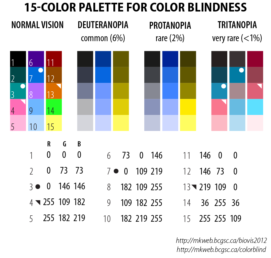
We acknowledge helpful conversations with Ana Bonaca, Blakesley Burkhart, Erin Cram, Tansu Daylan, Bruce Draine, Cora Dvorkin, Daniel Eisenstein, Daniel Foreman-Mackey, J. Colin Hill, John Kovac, Albert Lee, Karin Öberg, Stephen Portillo, Eddie Schlafly, Zachary Slepian, Josh Speagle, David Spergel, Justina Yang, Jun Yin and Catherine Zucker. IZ is supported by the Harvard College Observatory. DF is partially supported by National Science Foundation grant AST-1614941, ‘‘Exploring the Galaxy: 3-Dimensional Structure and Stellar Streams.’’ This research made use of the NASA Astrophysics Data System’s Bibliographic Services (ADS), the Odyssey Cluster at Harvard University, the color blindness palette by Martin Krzywinski and Jonathan Corum55 5 http://mkweb.bcgsc.ca/biovis2012/color-blindness-palette.png, and the Color Vision Deficiency PDF Viewer by Marie Chatfield 66 6 https://mariechatfield.com/simple-pdf-viewer/.
Appendix A Fisher Information Matrix Derivatives Calculation
This section contains the analytical forms of the function derivatives used for the Fisher information matrix calculations in §IV.
distortion
| (A1) |
y Distortion
| (A2) |
Blackbody Temperature Distortion
| (A3) |
ISM Dust Principal Components
| (A4) |
Synchrotron
| (A5) |
| (A6) |
| (A7) |
Cosmic Infrared Background
| (A8) |
| (A9) |
| (A10) |
Free-free Emission
| (A11) |
Appendix B Analytical Approximation to Gaussian Convolution
In this section we derive the analytical approximation to convolving a function with a Gaussian. We use a normal Gaussian because we do not want to scale the function up or down, but rather to just”smooth it over”. For our purposes, the mean of the Gaussian has to be zero, otherwise the convolution would shift the original function as well. The Gaussian is approximated using two functions77 7 If we only pick one function, it will have a zero standard deviation. So, we use two functions., in such a way that the resulting function has the same mean and standard deviation of the Gaussian. Because the amplitude of a delta function when integrated over an entire domain is one, we scale it by a factor of 2:
| (B1) |
We want to know what should be the offset such that the function has the same standard deviation as the Gaussian. Thus, the offset can be calculated as a function of the desired in the following manner:
| (B2) |
This proves that should be equal to . As a result, the approximation to the Gaussian will be given by:
| (B3) |
Now, the convolution of a function with the Gaussian approximation will be given by:
| (B4) |
where we make use of the relation .
We represent the function as a Taylor Series:
| (B5) |
| (B6) |
Thus, the convolution of a function with a Gaussian can be approximated by an expansion in even derivatives multiplied by the power terms of .
References
- Abitbol et al. (2017) Abitbol, M. H., Chluba, J., Hill, J. C., & Johnson, B. R. 2017, Monthly Notices of the Royal Astronomical Society, Volume 471, Issue 1, p.1126-1140, 471, 1126, doi: 10.1093/mnras/stx1653
- Bennett et al. (2003) Bennett, C. L., Hill, R. S., Hinshaw, G., et al. 2003, The Astrophysical Journal Supplement Series, Volume 148, Issue 1, pp. 97-117., 148, 97, doi: 10.1086/377252
- Boggess et al. (1992) Boggess, N. W., Mather, J. C., Weiss, R., et al. 1992, The Astrophysical Journal, 397, 420, doi: 10.1086/171797
- Burigana et al. (1991) Burigana, C., Danese, L., & de Zotti, G. 1991, Astronomy and Astrophysics, 246, 49. https://ui.adsabs.harvard.edu/abs/1991A{&}A...246...49B
- Chluba (2014) Chluba, J. 2014, Science with CMB spectral distortions. https://ui.adsabs.harvard.edu/abs/2014arXiv1405.6938C
- Chluba et al. (2017) Chluba, J., Hill, J. C., & Abitbol, M. H. 2017, Monthly Notices of the Royal Astronomical Society, 472, 1195, doi: 10.1093/mnras/stx1982
- Chluba & Jeong (2014) Chluba, J., & Jeong, D. 2014, Monthly Notices of the Royal Astronomical Society, Volume 438, Issue 3, p.2065-2082, 438, 2065, doi: 10.1093/mnras/stt2327
- Chluba et al. (2012) Chluba, J., Khatri, R., & Sunyaev, R. A. 2012, Monthly Notices of the Royal Astronomical Society, 425, 1129, doi: 10.1111/j.1365-2966.2012.21474.x
- Chluba & Sunyaev (2012) Chluba, J., & Sunyaev, R. A. 2012, Monthly Notices of the Royal Astronomical Society, Volume 419, Issue 2, pp. 1294-1314., 419, 1294, doi: 10.1111/j.1365-2966.2011.19786.x
- Chluba et al. (2019) Chluba, J., Kogut, A., Patil, S. P., et al. 2019, Bulletin of the American Astronomical Society, 51, 184. https://ui.adsabs.harvard.edu/abs/2019BAAS...51c.184C
- Collaboration (2014) Collaboration, P. 2014, Astronomy and Astrophysics, 571, A30, doi: 10.1051/0004-6361/201322093
- Draine (2011) Draine, B. T. 2011, Physics of the Interstellar and Intergalactic Medium. https://ui.adsabs.harvard.edu/abs/2011piim.book.....D
- Draine & Lee (1984) Draine, B. T., & Lee, H. M. 1984, Astrophysical Journal v.285, p.89, 285, 89, doi: 10.1086/162480
- Finkbeiner et al. (1999) Finkbeiner, D. P., Davis, M., & Schlegel, D. J. 1999, The Astrophysical Journal, Volume 524, Issue 2, pp. 867-886., 524, 867, doi: 10.1086/307852
- Fixsen (2009) Fixsen, D. J. 2009, The Astrophysical Journal, Volume 707, Issue 2, pp. 916-920 (2009)., 707, 916, doi: 10.1088/0004-637X/707/2/916
- Fixsen et al. (1996) Fixsen, D. J., Cheng, E. S., Gales, J. M., et al. 1996, Astrophysical Journal v.473, p.576, 473, 576, doi: 10.1086/178173
- Hauser & Dwek (2001) Hauser, M. G., & Dwek, E. 2001, Annual Review of Astronomy and Astrophysics, Vol. 39, p. 249-307 (2001)., 39, 249, doi: 10.1146/annurev.astro.39.1.249
- Hill et al. (2015) Hill, J. C., Battaglia, N., Chluba, J., et al. 2015, Physical Review Letters, Volume 115, Issue 26, id.261301, 115, 261301, doi: 10.1103/PhysRevLett.115.261301
- Hu & Silk (1993) Hu, W., & Silk, J. 1993, Physical Review D, 48, 485, doi: 10.1103/PhysRevD.48.485
- Hunter (2007) Hunter, J. D. 2007, Computing in Science and Engineering, 9, 90, doi: 10.1109/MCSE.2007.55
- Illarionov & Siuniaev (1975) Illarionov, A. F., & Siuniaev, R. A. 1975, Soviet Astronomy, vol. 18, Jan.-Feb. 1975, p. 413-419. Translation., 18, 413. https://ui.adsabs.harvard.edu/abs/1975SvA....18..413I
- Imara & Loeb (2016) Imara, N., & Loeb, A. 2016, The Astrophysical Journal, Volume 825, Issue 2, article id. 130, 7 pp. (2016)., 825, 130, doi: 10.3847/0004-637X/825/2/130
- Khatri & Sunyaev (2012) Khatri, R., & Sunyaev, R. A. 2012, Journal of Cosmology and Astroparticle Physics, Issue 09, article id. 016 (2012)., 2012, 16, doi: 10.1088/1475-7516/2012/09/016
- Kogut et al. (2016) Kogut, A., Chluba, J., Fixsen, D. J., Meyer, S., & Spergel, D. 2016, in Proceedings of the SPIE, Volume 9904, id. 99040W 23 pp. (2016)., Vol. 9904, 99040W, doi: 10.1117/12.2231090
- Kogut & Fixsen (2020) Kogut, A., & Fixsen, D. J. 2020, Journal of Cosmology and Astroparticle Physics, 2020, 41, doi: 10.1088/1475-7516/2020/05/041
- Kogut et al. (2011) Kogut, A., Fixsen, D. J., Chuss, D. T., et al. 2011, Journal of Cosmology and Astroparticle Physics, Issue 07, id. 025 (2011)., 2011, 25, doi: 10.1088/1475-7516/2011/07/025
- Laor & Draine (1993) Laor, A., & Draine, B. T. 1993, Astrophysical Journal v.402, p.441, 402, 441, doi: 10.1086/172149
- Lenz et al. (2019) Lenz, D., Doré, O., & Lagache, G. 2019, The Astrophysical Journal, 883, 75, doi: 10.3847/1538-4357/ab3c2b
- Li & Draine (2001) Li, A., & Draine, B. T. 2001, The Astrophysical Journal, Volume 554, Issue 2, pp. 778-802., 554, 778, doi: 10.1086/323147
- Mather et al. (1994) Mather, J. C., Cheng, E. S., Cottingham, D. A., et al. 1994, Astrophysical Journal v.420, p.439, 420, 439, doi: 10.1086/173574
- McKinney (2010) McKinney, W. 2010, in {P}roceedings of the 9th {P}ython in {S}cience {C}onference, ed. S. van der Walt & J. Millman, 56–61, doi: 10.25080/Majora-92bf1922-00a
- Millman & Aivazis (2011) Millman, K. J., & Aivazis, M. 2011, Computing in Science and Engineering, 13, 9, doi: 10.1109/MCSE.2011.36
- Næss et al. (2019) Næss, S. K., Dunkley, J., Kogut, A., & Fixsen, D. J. 2019, Journal of Cosmology and Astroparticle Physics, 2019, 19, doi: 10.1088/1475-7516/2019/04/019
- Nashimoto et al. (2020) Nashimoto, M., Hattori, M., & Chinone, Y. 2020, The Astrophysical Journal, 895, L21, doi: 10.3847/2041-8213/ab9018
- Oliphant (2007) Oliphant, T. E. 2007, Computing in Science and Engineering, 9, 10, doi: 10.1109/MCSE.2007.58
- Pedregosa et al. (2012) Pedregosa, F., Varoquaux, G., Gramfort, A., et al. 2012, Scikit-learn: Machine Learning in Python. https://ui.adsabs.harvard.edu/abs/2012arXiv1201.0490P
- Perez & Granger (2007) Perez, F., & Granger, B. E. 2007, Computing in Science and Engineering, 9, 21, doi: 10.1109/MCSE.2007.53
- Planck Collaboration (2014) Planck Collaboration. 2014, Astronomy and Astrophysics, 571, A11, doi: 10.1051/0004-6361/201323195
- Planck Collaboration (2016a) —. 2016a, Astronomy and Astrophysics, 594, A10, doi: 10.1051/0004-6361/201525967
- Planck Collaboration (2016b) —. 2016b, Astronomy and Astrophysics, 596, A104, doi: 10.1051/0004-6361/201628522
- Planck Collaboration (2016c) —. 2016c, Astronomy and Astrophysics, 596, A109, doi: 10.1051/0004-6361/201629022
- Reach et al. (1995) Reach, W. T., Dwek, E., Fixsen, D. J., et al. 1995, Astrophysical Journal v.451, p.188, 451, 188, doi: 10.1086/176210
- Remazeilles & Chluba (2020) Remazeilles, M., & Chluba, J. 2020, Monthly Notices of the Royal Astronomical Society, 494, 5734, doi: 10.1093/mnras/staa1135
- Rotti & Chluba (2021) Rotti, A., & Chluba, J. 2021, Monthly Notices of the Royal Astronomical Society, 500, 976, doi: 10.1093/mnras/staa3292
- Sazonov & Sunyaev (1998) Sazonov, S. Y., & Sunyaev, R. A. 1998, The Astrophysical Journal, Volume 508, Issue 1, pp. 1-5., 508, 1, doi: 10.1086/306406
- Schlafly et al. (2016) Schlafly, E. F., Meisner, A. M., Stutz, A. M., et al. 2016, apj, 821, 78, doi: 10.3847/0004-637X/821/2/78
- Shlens (2014) Shlens, J. 2014, A Tutorial on Principal Component Analysis. https://ui.adsabs.harvard.edu/abs/2014arXiv1404.1100S
- Sunyaev & Zeldovich (1970) Sunyaev, R. A., & Zeldovich, Y. B. 1970, Astrophysics and Space Science, 7, 20, doi: 10.1007/BF00653472
- Sunyaev & Zeldovich (1972) —. 1972, Astronomy and Astrophysics, 20, 189. https://ui.adsabs.harvard.edu/abs/1972A{&}A....20..189S
- Tashiro (2014) Tashiro, H. 2014, Progress of Theoretical and Experimental Physics, Volume 2014, Issue 6, id.06B10727 pp., 2014, 06B107, doi: 10.1093/ptep/ptu066
- van der Walt et al. (2011) van der Walt, S., Colbert, S. C., & Varoquaux, G. 2011, Computing in Science and Engineering, 13, 22, doi: 10.1109/MCSE.2011.37
- Verde (2010) Verde, L. 2010, in Lectures on Cosmology Accelerated Expansion of the Universe by Georg Wolschin, Lecture Notes in Physics vol. 800, Springer Berlin / Heidelberg, ISSN 1616-6361; ISBN 978-3-642-10597-5, pp.147-177, Vol. 800, 147–177, doi: 10.1007/978-3-642-10598-2_4
- Vousden et al. (2016) Vousden, W. D., Farr, W. M., & Mandel, I. 2016, Monthly Notices of the Royal Astronomical Society, 455, 1919, doi: 10.1093/mnras/stv2422
- Weingartner & Draine (2001) Weingartner, J. C., & Draine, B. T. 2001, The Astrophysical Journal, Volume 548, Issue 1, pp. 296-309., 548, 296, doi: 10.1086/318651
- Wright (1991) Wright, E. L. 1991, The Astrophysical Journal, 375, 608, doi: 10.1086/170222
- Zeldovich & Sunyaev (1969) Zeldovich, Y. B., & Sunyaev, R. A. 1969, Astrophysics and Space Science, 4, 301, doi: 10.1007/BF00661821
- Zelko (2021) Zelko, I. 2021, Dust Spectral Energy Distribution Data from Zelko & Finkbeiner 2020a and 2020b, Harvard Dataverse, doi: doi:10.7910/DVN/DJAAIG
- Zelko & Finkbeiner (2020) Zelko, I. A., & Finkbeiner, D. P. 2020, ApJ, 904, 38, doi: 10.3847/1538-4357/abbb8d