跳到论文正文
W Papers独立论文阅读器 arXiv:2010.06392 论文正文 计算阅读时间 · 0%
引用这篇论文根据当前论文元数据生成,正式投稿前建议核对。


License: CC BY-NC-SA 4.0
arXiv:2010.06392v1 [math.NA] 13 Oct 2020

Projection techniques to update the truncated SVD of evolving matrices

Vassilis Kalantzis Thanks: IBM Research, Thomas J. Watson Research Center, Yorktown Heights, NY 10598, US. Email: vkal@ibm.com    Georgios Kollias Thanks: IBM Research, Thomas J. Watson Research Center, Yorktown Heights, NY 10598, US. Email: gkollias@us.ibm.com    Shashanka Ubaru Thanks: IBM Research, Thomas J. Watson Research Center, Yorktown Heights, NY 10598, US. Email: shashanka.ubaru@us.ibm.com    Athanasios N. Nikolakopoulos Thanks: University of Minnesota, Minneapolis, MN 55455, US. Email: anikolak@umn.edu    Lior Horesh Thanks: IBM Research, Thomas J. Watson Research Center, Yorktown Heights, NY 10598, US. Email: lhoresh@us.ibm.com    Kenneth L. Clarkson Thanks: IBM Research, Almaden Research Center, San Jose, CA 95120, US. Email: klclarks@us.ibm.com
Abstract

This paper considers the problem of updating the rank-kk truncated Singular Value Decomposition (SVD) of matrices subject to the addition of new rows and/or columns over time. Such matrix problems represent an important computational kernel in applications such as Latent Semantic Indexing and Recommender Systems. Nonetheless, the proposed framework is purely algebraic and targets general updating problems. The algorithm presented in this paper undertakes a projection viewpoint and focuses on building a pair of subspaces which approximate the linear span of the sought singular vectors of the updated matrix. We discuss and analyze two different choices to form the projection subspaces. Results on matrices from real applications suggest that the proposed algorithm can lead to higher accuracy, especially for the singular triplets associated with the largest modulus singular values. Several practical details and key differences with other approaches are also discussed.

Keywords:

Singular Value Decomposition, evolving matrices, Lanczos bidiagonalization, latent semantic analysis, recommender systems

1 Introduction

This paper considers the update of the truncated SVD of a sparse matrix subject to additions of new rows and/or columns. More specifically, let B∈ℂm×nB\in\mathbb{C}^{m\times n} be a matrix for which its rank-kk (truncated) SVD BkB_{k} is available. Our goal is to obtain an approximate rank-kk SVD AkA_{k} of matrix

A=(BE),orA=(BE),A=\begin{pmatrix}B\\[3.00003pt] E\\[3.00003pt] \end{pmatrix},\ \ {\rm or}\ \ A=\begin{pmatrix}B&E\end{pmatrix},

where EE denotes the matrix of newly added rows or columns. This process can be repeated several times, where at each instance matrix AA becomes matrix BB at the next level. Note that a similar problem, not explored in this paper, is to approximate the rank-kk SVD of BB after modifying its (non-)zero entries, e.g., see [31].

Matrix problems such as the ones above hold an important role in several real-world applications. One such example is Latent Semantic Indexing (LSI) in which the truncated SVD of the current term-document matrix needs to be updated after a few new terms/documents have been added to the collection [3, 7, 31]. Another example is the update of latent-factor-based models of user-item rating matrices in top-N recommendation [6, 19, 23]. Additional applications in geostatistical screening can be found in [13, Chapter 6].

The standard approach to compute AkA_{k} is to disregard any previously available information and apply directly to AA an off-the-shelf, high-performance, SVD solver [2, 12, 29, 10, 27]. This standard approach might be feasible when the original matrix is updated only once or twice, however becomes increasingly impractical as multiple row/column updates take place over time. Therefore, it becomes crucial to develop algorithms which return a reasonable approximation of AkA_{k} while taking advantage of BkB_{k}. Such schemes have already been considered extensively for the case of full SVD [4, 9, 17] and rank-kk SVD [3, 23, 28, 31]. Nonetheless, for general-purpose matrices it is rather unclear how to enhance their accuracy.

1.1 Contributions.

  1. 1.

    We propose and analyze a projection scheme to update the rank-kk SVD of evolving matrices. Our scheme uses a right singular projection subspace equal to ℂn\mathbb{C}^{n}, and only determines the left singular projection subspace.

  2. 2.

    We propose and analyze two different options to set the left singular projection subspace. A complexity analysis is also presented.

  3. 3.

    We present experiments performed on matrices stemming from applications in LSI and recommender systems. These experiments demonstrate the numerical behavior of the proposed scheme and showcase the various tradeoffs in accuracy versus complexity.

2 Background and notation

The (full) SVD of matrix BB is denoted as B=U​Σ​VHB=U\Sigma V^{H} where U∈ℂm×mU\in\mathbb{C}^{m\times m} and V∈ℂn×nV\in\mathbb{C}^{n\times n} are unitary matrices whose jj’th column is equal to the left singular vector u(j)u^{(j)} and right singular vector v(j)v^{(j)}, respectively. The matrix Σ∈ℝm×n\Sigma\in\mathbb{R}^{m\times n} has non-zero entries only along its main diagonal, and these entries are equal to the singular values σ1≥⋯≥σ𝚖𝚒𝚗⁡(m,n)\sigma_{1}\geq\cdots\geq\sigma_{\mathtt{min}(m,n)}. Moreover, we define the matrices Uj=[u(1),…,u(j)]U_{j}=\left[u^{(1)},\ldots,u^{(j)}\right], Vj=[v(1),…,v(j)]V_{j}=\left[v^{(1)},\ldots,v^{(j)}\right], and Σj=𝚍𝚒𝚊𝚐⁡(σ1,…,σj)\Sigma_{j}=\mathtt{diag}\left(\sigma_{1},\ldots,\sigma_{j}\right). The rank-kk truncated SVD of matrix BB can then be written as Bk=Uk​Σk​VkH=∑j=1kσj​u(j)​(v(j))HB_{k}=U_{k}\Sigma_{k}V_{k}^{H}=\sum_{j=1}^{k}\sigma_{j}u^{(j)}\left(v^{(j)}\right)^{H}. We follow the same notation for matrix AA with the exception that a circumflex is added on top of each variable, i.e., Ak=U^k​Σ^k​V^kH=∑j=1kσ^j​u^(j)​(v^(j))HA_{k}=\widehat{U}_{k}\widehat{\Sigma}_{k}\widehat{V}_{k}^{H}=\sum_{j=1}^{k}\widehat{\sigma}_{j}\widehat{u}^{(j)}\left(\widehat{v}^{(j)}\right)^{H}, with U^j=[u^(1),…,u^(j)]\widehat{U}_{j}=\left[\widehat{u}^{(1)},\ldots,\widehat{u}^{(j)}\right], V^j=[v^(1),…,v^(j)]\widehat{V}_{j}=\left[\widehat{v}^{(1)},\ldots,\widehat{v}^{(j)}\right], and Σ^j=𝚍𝚒𝚊𝚐⁡(σ^1,…,σ^j)\widehat{\Sigma}_{j}=\mathtt{diag}\left(\widehat{\sigma}_{1},\ldots,\widehat{\sigma}_{j}\right).

The routines 𝚗𝚛⁡(K)\mathtt{nr}(K) and 𝚗𝚗𝚣⁡(K)\mathtt{nnz}(K) return the number of rows of matrix and non-zero entries of matrix KK, respectively. Throughout this paper ∥⋅∥\|\cdot\| will stand for the ℓ2\ell_{2} norm when the input is a vector, and the spectral norm when the input is a matrix. Moreover, the term 𝚛𝚊𝚗𝚐𝚎⁡(K)\mathtt{range}(K) will denote the column space of matrix KK, while 𝚜𝚙𝚊𝚗⁡(⋅)\mathtt{span}(\cdot) will denote the linear span of a set of vectors. The identity matrix of size nn will be denoted by InI_{n}.

2.1 Related work.

The problem of updating the SVD of an evolving matrix has been considered extensively in the context of LSI. Consider first the case A=(BE)A=\begin{pmatrix}B\\ E\\ \end{pmatrix}, and let (I−Vk​VkH)​EH=Q​R(I-V_{k}V_{k}^{H})E^{H}=QR such that QQ is orthonormal and RR is upper trapezoidal. The scheme in [31] writes

(BE)≈(Uk​Σk​VkHE)\displaystyle\begin{pmatrix}B\\[2.77501pt] E\\[2.77501pt] \end{pmatrix}\approx\begin{pmatrix}U_{k}\Sigma_{k}V_{k}^{H}\\[2.77501pt] E\\[2.77501pt] \end{pmatrix} =\displaystyle= (UkIs)​(ΣkE​VkRH)​(VkQ)H\displaystyle\begin{pmatrix}U_{k}&\\[2.77501pt] &I_{s}\\[2.77501pt] \end{pmatrix}\begin{pmatrix}\Sigma_{k}&\\[2.77501pt] EV_{k}&R^{H}\\[2.77501pt] \end{pmatrix}\begin{pmatrix}V_{k}&Q\\[2.77501pt] \end{pmatrix}^{H}
=\displaystyle= ((UkIs)​F)​Θ​((VkQ)​G)H\displaystyle\left(\begin{pmatrix}U_{k}&\\[2.77501pt] &I_{s}\\[2.77501pt] \end{pmatrix}F\right)\Theta\left(\begin{pmatrix}V_{k}&Q\\[2.77501pt] \end{pmatrix}G\right)^{H}

where the matrix product F​Θ​GHF\Theta G^{H} denotes the compact SVD of the matrix (ΣkE​VkRH)\begin{pmatrix}\Sigma_{k}&\\ EV_{k}&R^{H}\\ \end{pmatrix}.

The above idea can be also applied to A=(BE)A=\begin{pmatrix}B&E\end{pmatrix}. Indeed, if matrices QQ and RR are now determined as (I−Uk​UkH)​E=Q​R(I-U_{k}U_{k}^{H})E=QR, we can approximate

(BE)\displaystyle\begin{pmatrix}B&E\end{pmatrix} ≈\displaystyle\approx (Uk​Σk​VkHE)\displaystyle\begin{pmatrix}U_{k}\Sigma_{k}V_{k}^{H}&E\end{pmatrix}
=\displaystyle= (UkQ)​(ΣkUkH​ER)​(VkHIs)\displaystyle\begin{pmatrix}U_{k}&Q\end{pmatrix}\begin{pmatrix}\Sigma_{k}&U_{k}^{H}E\\[2.77501pt] &R\\[2.77501pt] \end{pmatrix}\begin{pmatrix}V_{k}^{H}&\\[2.77501pt] &I_{s}\\[2.77501pt] \end{pmatrix}
=\displaystyle= ((UkQ)​F)​Θ​((VkIs)​G)H\displaystyle\left(\begin{pmatrix}U_{k}&Q\end{pmatrix}F\right)\Theta\left(\begin{pmatrix}V_{k}&\\[2.77501pt] &I_{s}\\[2.77501pt] \end{pmatrix}G\right)^{H}

where the matrix product F​Θ​GF\Theta G now denotes the compact SVD of the matrix (ΣkUkH​ER)\begin{pmatrix}\Sigma_{k}&U_{k}^{H}E\\ &R\\ \end{pmatrix}.

When BkB_{k} coincides with the compact SVD of BB, the above schemes compute the exact rank-kk SVD of AA, and no access to matrix BB is required. Nonetheless, the application of the method in [31] can be challenging. For general updating problems, or problems where AA does not satisfy a “low-rank plus shift” structure [32], replacing BB by BkB_{k} might not lead to a satisfactory approximation of AkA_{k}. Moreover, the memory/computational cost associated with the computation of the QR and SVD decompositions in each one of the above two scenarios might be prohibitive. The latter was recognized in [28] where it was proposed to adjust the method in [31] by replacing matrices (I−Vk​VkH)​EH(I-V_{k}V_{k}^{H})E^{H} and (I−Uk​UkH)​E(I-U_{k}U_{k}^{H})E with a low-rank approximation computed by applying the Golub-Kahan Lanczos bidiagonalization procedure [8]. Similar ideas have been suggested in [30] and [26] where the Golub-Kahan Lanczos bidiagonalization procedure was replaced by randomized SVD [10, 25] and graph coarsening [26], respectively.

3 The projection viewpoint

The methods discussed in the previous section can be recognized as instances of a Rayleigh-Ritz projection procedure and can be summarized as follows [28, 30]:

  1. 1.

    Compute matrices ZZ and WW such that 𝚛𝚊𝚗𝚐𝚎⁡(Z)\mathtt{range}(Z) and 𝚛𝚊𝚗𝚐𝚎⁡(WH)\mathtt{range}(W^{H}) approximately capture 𝚛𝚊𝚗𝚐𝚎⁡(U^k)\mathtt{range}(\widehat{U}_{k}) and 𝚛𝚊𝚗𝚐𝚎⁡(V^kH)\mathtt{range}(\widehat{V}_{k}^{H}), respectively.

  2. 2.

    Compute [Θk,Fk,Gk]=𝚜𝚟𝚍⁡(ZH​A​W)[\Theta_{k},F_{k},G_{k}]=\mathtt{svd}(Z^{H}AW) where Θk,Fk\Theta_{k},\ F_{k}, and GkG_{k} denote the kk leading singular values and associated left and right singular vectors of ZH​A​WZ^{H}AW, respectively.

  3. 3.

    Approximate AkA_{k} by the product (Z​Fk)​Θk​(W​Gk)H(ZF_{k})\Theta_{k}(WG_{k})^{H}.

Ideally, the matrices ZZ and WW should satisfy

𝚜𝚙𝚊𝚗⁡(u^(1),…,u^(k))\displaystyle\mathtt{span}\left(\widehat{u}^{(1)},\ldots,\widehat{u}^{(k)}\right) ⊆\displaystyle\subseteq 𝚛𝚊𝚗𝚐𝚎⁡(Z),and\displaystyle\mathtt{range}(Z),\ \ \rm{and}
𝚜𝚙𝚊𝚗⁡(v^(1),…,v^(k))\displaystyle\mathtt{span}\left(\widehat{v}^{(1)},\ldots,\widehat{v}^{(k)}\right) ⊆\displaystyle\subseteq 𝚛𝚊𝚗𝚐𝚎⁡(W).\displaystyle\mathtt{range}(W).

Moreover, the size of matrix ZH​A​WZ^{H}AW should be as small as possible to avoid high computational costs during the computation of [Θk,Fk,Gk]=𝚜𝚟𝚍⁡(ZH​A​W)[\Theta_{k},F_{k},G_{k}]=\mathtt{svd}(Z^{H}AW).

Table 1 summarizes a few options to set matrices ZZ and WW for the row updating problem. The method in [28] considers the same matrix ZZ as in [31] but sets W=[Vk,Xr]W=[V_{k},X_{r}] where XrX_{r} denotes the r∈ℤ∗r\in\mathbb{Z}^{*} leading left singular vectors of (I−Vk​VkH)​EH(I-V_{k}V_{k}^{H})E^{H}. The choice of matrices ZZ and WW listed under the option “Algorithm 1” is explained in the next section. Note that the first variant of Algorithm 1 uses the same ZZ as in [31] and [28] but different WW. This choice leads to similar or higher accuracy than the scheme in [31] and this is also achieved asymptotically faster. A detailed comparison is deferred to the Supplementary Material. The second variant of Algorithm 1 is a more expensive but also more accurate version of the first variant.

Table 1: Different options to set the projection matrices ZZ and WW for the row updating problem.
Method ZZ WW
[3] VkV_{k}
[31] Z=(UkIs)Z=\begin{pmatrix}U_{k}&\\ &I_{s}\\ \end{pmatrix} [Vk,Q][V_{k},Q]
[28] [Vk,Xr][V_{k},X_{r}]
Alg. 1 Z=(UkIs)Z=\begin{pmatrix}U_{k}&\\ &I_{s}\\ \end{pmatrix} InI_{n}
Alg. 1 Z=(Uk,Xλ,rIs)Z=\begin{pmatrix}U_{k},X_{\lambda,r}&\\ &I_{s}\\ \end{pmatrix} InI_{n}

3.1 The proposed algorithm.

Consider again the SVD update of matrix A=(BE)A=\begin{pmatrix}B\\ E\\ \end{pmatrix}, with E∈ℂs×nE\in\mathbb{C}^{s\times n}. The right singular vectors of AA trivially satisfy v^(i)⊆𝚛𝚊𝚗𝚐𝚎(In),i=1,…,n\widehat{v}^{(i)}\subseteq\mathtt{range}(I_{n}),\ i=1,\ldots,n. Therefore, we can simply set W=InW=I_{n} and compute the kk leading singular triplets (θi,f(i),g(i))\left(\theta_{i},f^{(i)},g^{(i)}\right) of the matrix ZH​A​W=ZH​AZ^{H}AW=Z^{H}A. Indeed, this choice of WW is ideal in terms of accuracy while it also removes the need to compute an approximate factorization of matrix (I−Vk​VkH)​EH(I-V_{k}V_{k}^{H})E^{H}. On the other hand, the number of columns in matrix ZH​A​WZ^{H}AW is now equal to nn instead of k+sk+s in [31] and k+l,l≪sk+l,\ l\ll s, in [28, 30]. This difference can be important when the full SVD of ZH​A​WZ^{H}AW is computed as in [28, 30, 31].

Our approach is to compute the singular values of ZH​AZ^{H}A in a matrix-free fashion while also skipping the computation of the right singular vectors GkG_{k}. Indeed, the matrix GkG_{k} is only needed to approximate the kk leading singular vectors V^k\widehat{V}_{k} of AA. Assuming that an approximation U¯k\overline{U}_{k} and Σ¯k\overline{\Sigma}_{k} of the matrices U^k\widehat{U}_{k} and Σ^k\widehat{\Sigma}_{k} is available, V^k\widehat{V}_{k} can be approximated as V¯k=AH​U¯k​Σ¯k−1\overline{V}_{k}=A^{H}\overline{U}_{k}\overline{\Sigma}_{k}^{-1}.

Algorithm 1 RR-SVD (“A​AHAA^{H}” version).
1: Input: B,Uk,Σk,Vk,E,ZB,U_{k},\Sigma_{k},V_{k},E,Z
2: Output: U¯k≈U^k,Σ¯k≈Σ^k,V¯k≈V^k\overline{U}_{k}\approx\widehat{U}_{k},\overline{\Sigma}_{k}\approx\widehat{\Sigma}_{k},\overline{V}_{k}\approx\widehat{V}_{k}
3: Solve [Θk,Fk]=𝚜𝚟𝚍k​(ZH​A)[\Theta_{k},F_{k}]=\mathtt{svd}_{k}(Z^{H}A)
4: Set U¯k=Z​Fk\overline{U}_{k}=ZF_{k} and Σ¯k=Θk\overline{\Sigma}_{k}=\Theta_{k}
5: Set V¯k=AH​U¯k​Σ¯k−1\overline{V}_{k}=A^{H}\overline{U}_{k}\overline{\Sigma}_{k}^{-1}

The proposed method is sketched in Algorithm 1. In terms of computational cost, Steps 4 and 5 require approximately 2​𝚗𝚗𝚣​(Z)​k2\mathtt{nnz}(Z)k and (2​𝚗𝚗𝚣​(A)+n)​k(2\mathtt{nnz}(A)+n)k Floating Point Operations (FLOPs), respectively. The complexity of Step 3 will generally depend on the algorithm used to compute the matrices Θk\Theta_{k} and FkF_{k}. We assume that these are computed by applying the unrestarted Lanczos method to matrix ZH​A​AH​ZZ^{H}AA^{H}Z in a matrix-free fashion [21]. Under the mild assumption that Lanczos performs δ\delta iterations for some δ∈ℤ∗\delta\in\mathbb{Z}^{*} which is greater than or equal to kk, a rough estimate of the total computational cost of Step 3 is 4​(𝚗𝚗𝚣⁡(ZH)+𝚗𝚗𝚣⁡(A))​δ+2​𝚗𝚛​(ZH)​δ24\left(\mathtt{nnz}(Z^{H})+\mathtt{nnz}(A)\right)\delta+2\mathtt{nr}(Z^{H})\delta^{2} FLOPs. The exact complexity of Lanczos will depend on the choice of matrix ZZ. A detailed asymptotic analysis of the complexity of Algorithm 1 and comparisons with other schemes are deferred to the Supplemental.

Algorithm 2 RR-SVD (“AH​AA^{H}A” version).
1: Input: B,Uk,Σk,Vk,E,ZB,U_{k},\Sigma_{k},V_{k},E,Z
2: Output: U¯k≈U^k,Σ¯k≈Σ^k,V¯k≈V^k\overline{U}_{k}\approx\widehat{U}_{k},\overline{\Sigma}_{k}\approx\widehat{\Sigma}_{k},\overline{V}_{k}\approx\widehat{V}_{k}
3: Solve [Θk,Gk]=𝚜𝚟𝚍k​(ZH​AH)[\Theta_{k},G_{k}]=\mathtt{svd}_{k}(Z^{H}A^{H})
4: Set V¯k=Z​Gk\overline{V}_{k}=ZG_{k} and Σ¯k=Θk\overline{\Sigma}_{k}=\Theta_{k}
5: Set U¯k=A​V¯k​Σ¯k−1\overline{U}_{k}=A\overline{V}_{k}\overline{\Sigma}_{k}^{-1}

Algorithm 1 can be adapted to approximate AkA_{k} for matrices of the form A=(BE)A=\begin{pmatrix}B&E\end{pmatrix}. The complete procedure is summarized in Algorithm 2. Note that by combining Algorithms 1 and 2 we can approximate the kk leading singular triplets of matrices in which we add both new rows and columns.

Throughout the remainder of this paper we focus in updating the rank-kk SVD of matrix A=(BE)A=\begin{pmatrix}B\\ E\\ \end{pmatrix} by Algorithm 1. The discussion extends trivially to updates of matrix A=(BE)A=\begin{pmatrix}B&E\end{pmatrix} by Algorithm 2.

4 Building the projection matrix ZZ

The accuracy of Step 5 in Algorithm 1 depends on the accuracy of the approximate leading singular values and associated left singular vectors from Step 3. In turn, these quantities depend on how well 𝚛𝚊𝚗𝚐𝚎⁡(Z)\mathtt{range}(Z) captures the singular vectors u^(1),…,u^(k)\widehat{u}^{(1)},\ldots,\widehat{u}^{(k)} [14, 18]. Therefore, our focus lies in forming ZZ such that the distance between the subspace 𝚛𝚊𝚗𝚐𝚎⁡(Z)\mathtt{range}(Z) and the left singular vectors u^(1),…,u^(k)\widehat{u}^{(1)},\ldots,\widehat{u}^{(k)} is as small as possible.

4.1 Exploiting the left singular vectors of BB.

The following proposition presents a closed-form expression of the ii’th left singular vector of matrix A=(BE)A=\begin{pmatrix}B\\ E\\ \end{pmatrix}.

Proposition 4.1

The left singular vector u^(i)\widehat{u}^{(i)} associated with singular value σ^i\widehat{\sigma}_{i} is equal to

u^(i)=(−(B​BH−σ^i2​Im)−1​B​EH​y^(i)y^(i)),\widehat{u}^{(i)}=\begin{pmatrix}-(BB^{H}-\widehat{\sigma}_{i}^{2}I_{m})^{-1}BE^{H}\widehat{y}^{(i)}\\[3.00003pt] \widehat{y}^{(i)}\\[3.00003pt] \end{pmatrix},

where y^(i)\widehat{y}^{(i)} satisfies the equation

[E⁡(∑j=1nv(j)​(v(j))H​σ^i2σ^i2−σj2)​EH−σ^i2​Is]​y^(i)=0,\left[E\left(\sum\limits_{j=1}^{n}v^{(j)}\left(v^{(j)}\right)^{H}\dfrac{\widehat{\sigma}_{i}^{2}}{\widehat{\sigma}_{i}^{2}-\sigma_{j}^{2}}\right)E^{H}-\widehat{\sigma}_{i}^{2}I_{s}\right]\widehat{y}^{(i)}=0,

and σj=0\sigma_{j}=0 for any j=m+1,…,nj=m+1,\ldots,n (when n>mn>m).

Deferred to the Supplementary Material.           The above representation of u^(i)\widehat{u}^{(i)} requires the solution of a nonlinear eigenvalue problem to compute y^(i)\widehat{y}^{(i)}. Alternatively, we can express u^(i)\widehat{u}^{(i)} as follows.

Proposition 4.2

The left singular vector u^(i)\widehat{u}^{(i)} associated with singular value σ^i\widehat{\sigma}_{i} is equal to

u^(i)=(u(1),…,u(𝚖𝚒𝚗⁡(m,n))Is)​(χ1,iχ𝚖𝚒𝚗⁡(m,n),iy^(i)),\widehat{u}^{(i)}=\begin{pmatrix}u^{(1)},\ldots,u^{(\mathtt{min}(m,n))}&\\[3.00003pt] &I_{s}\\[3.00003pt] \end{pmatrix}\begin{pmatrix}\chi_{1,i}\\[3.00003pt] \vdots\\[3.00003pt] \chi_{\mathtt{min}(m,n),i}\\[3.00003pt] \widehat{y}^{(i)}\\[3.00003pt] \end{pmatrix},

where the scalars χj,i\chi_{j,i} are equal to

χj,i=−(E​v(j))H​y^(i)​σjσj2−σ^i2.\chi_{j,i}=-\left(Ev^{(j)}\right)^{H}\widehat{y}^{(i)}\dfrac{\sigma_{j}}{\sigma_{j}^{2}-\widehat{\sigma}_{i}^{2}}.

Deferred to the Supplementary Material.           Proposition 4.2 suggests that setting Z=(u(1),…,u(𝚖𝚒𝚗⁡(m,n))Is)Z=\begin{pmatrix}u^{(1)},\ldots,u^{(\mathtt{min}(m,n))}&\\ &I_{s}\\ \end{pmatrix} should lead to an exact (in the absence of round-off errors) computation of u^(i)\widehat{u}^{(i)}. In practice, we only have access to the kk leading left singular vectors of BB, u(1),…,u(k)u^{(1)},\ldots,u^{(k)}. The following proposition suggests that the distance between u^(i)\widehat{u}^{(i)} and the range space of Z=(u(1),…,u(k)Is)Z=\begin{pmatrix}u^{(1)},\ldots,u^{(k)}&\\ &I_{s}\\ \end{pmatrix} is at worst proportional to the ratio σk+1σk+12−σ^i2\dfrac{\sigma_{k+1}}{\sigma_{k+1}^{2}-\widehat{\sigma}_{i}^{2}}.

Proposition 4.3

Let matrix ZZ in Algorithm 1 be defined as

Z=(u(1),…,u(k)Is),Z=\begin{pmatrix}u^{(1)},\ldots,u^{(k)}&\\[3.00003pt] &I_{s}\\[3.00003pt] \end{pmatrix},

and set γ=O⁡(‖EH​y^(i)‖)\gamma=O\left(\left\lVert E^{H}\widehat{y}^{(i)}\right\rVert\right).

Then, for any i=1,…,ki=1,\ldots,k:

𝚖𝚒𝚗z∈𝚛𝚊𝚗𝚐𝚎⁡(Z)​‖u^(i)−z‖≤|γ​σk+1σk+12−σ^i2|.\mathtt{min}_{z\in\mathtt{range}(Z)}\|\widehat{u}^{(i)}-z\|\leq\left|\dfrac{\gamma\sigma_{k+1}}{\sigma_{k+1}^{2}-\widehat{\sigma}_{i}^{2}}\right|.

Deferred to the Supplementary Material.           Proposition 4.3 implies that left singular vectors associated with larger singular values of AA are likely to be approximated more accurately.

4.1.1 The structure of matrix ZH​AZ^{H}A.

Setting the projection matrix ZZ as in Proposition 4.3 gives

ZH​A=(Vk​ΣkEH)H.Z^{H}A=\begin{pmatrix}V_{k}\Sigma_{k}&E^{H}\end{pmatrix}^{H}.

Therefore, each Matrix-Vector (MV) product with matrix ZH​A​AH​ZZ^{H}AA^{H}Z requires two MV products with matrices Σk,Vk\Sigma_{k},\ V_{k} and EE, for a total cost of about 4​(n​k+𝚗𝚗𝚣​(E))4(nk+\mathtt{nnz}(E)) FLOPs. Moreover, we have 𝚗𝚛⁡(ZH)=s+k\mathtt{nr}(Z^{H})=s+k, and thus a rough estimate of the cost of Step 3 in Algorithm 1 is 4​(n​k+𝚗𝚗𝚣⁡(E))​δ+2​(s+k)​δ24(nk+\mathtt{nnz}(E))\delta+2(s+k)\delta^{2} FLOPs.

4.2 Exploiting resolvent expansions.

The choice of ZZ presented in Section 4.1 can compute the exact AkA_{k} provided that the rank of BB is exactly kk. Nonetheless, when the rank of BB is larger than kk and the singular values σk+1,…,σ𝚖𝚒𝚗⁡(m,n)\sigma_{k+1},\ldots,\sigma_{\mathtt{min}(m,n)} are not small, the accuracy of the approximate AkA_{k} returned by Algorithm 1 might be poor. This section presents an approach to enhance the projection matrix ZZ.

Recall that the top part of u^(i)\widehat{u}^{(i)} is equal to f^(i)=−(B​BH−σ^i2​Im)−1​B​EH​y^(i)\widehat{f}^{(i)}=-(BB^{H}-\widehat{\sigma}_{i}^{2}I_{m})^{-1}BE^{H}\widehat{y}^{(i)}. In practice, even if we knew the unknown quantities σ^i2\widehat{\sigma}_{i}^{2} and y^(i)\widehat{y}^{(i)}, the application of matrix (B​BH−σ^i2​Im)−1(BB^{H}-\widehat{\sigma}_{i}^{2}I_{m})^{-1} for each i=1,…,ki=1,\ldots,k, is too costly. The idea presented in this section considers the approximation of (B​BH−σ^i2​Im)−1,i=1,…,k(BB^{H}-\widehat{\sigma}_{i}^{2}I_{m})^{-1},\ i=1,\ldots,k, by (B​BH−λ​Im)−1(BB^{H}-\lambda I_{m})^{-1} for some fixed scalar λ∈ℝ\lambda\in\mathbb{R}.

Lemma 4.1

Let

B⁡(λ)=(Im−Uk​UkH)​(B​BH−λ​Im)−1B(\lambda)=(I_{m}-U_{k}U_{k}^{H})(BB^{H}-\lambda I_{m})^{-1}

such that λ>σ^k2\lambda>\widehat{\sigma}_{k}^{2}. Then, we have that for any i=1,…,ki=1,\ldots,k:

B⁡(σ^i2)=B⁡(λ)​∑ρ=0∞[(σ^i2−λ)​B​(λ)]ρ.B(\widehat{\sigma}_{i}^{2})=B(\lambda)\sum\limits_{\rho=0}^{\infty}\left[(\widehat{\sigma}_{i}^{2}-\lambda)B(\lambda)\right]^{\rho}.

Deferred to the Supplementary Material.           Clearly, the closer λ\lambda is to σ^i2\widehat{\sigma}_{i}^{2}, the more accurate the approximation in Lemma 4.1 should be. We can now provide an expression for u^(i)\widehat{u}^{(i)} similar to that in Proposition 4.2.

Proposition 4.4

The left singular vector u^(i)\widehat{u}^{(i)} associated with singular value σ^i\widehat{\sigma}_{i} is equal to

u^(i)\displaystyle\widehat{u}^{(i)} =\displaystyle= (u(1),…,u(k)Is)​(χ1,iχk,iy^(i))\displaystyle\begin{pmatrix}u^{(1)},\ldots,u^{(k)}&\\[3.00003pt] &I_{s}\\[3.00003pt] \end{pmatrix}\begin{pmatrix}\chi_{1,i}\\[3.00003pt] \vdots\\[3.00003pt] \chi_{k,i}\\[3.00003pt] \widehat{y}^{(i)}\\[3.00003pt] \end{pmatrix}
−(B⁡(λ)​∑ρ=0∞[(σ^i2−λ)​B​(λ)]ρ​B​EH​y^(i)).\displaystyle-\begin{pmatrix}B(\lambda)\sum\limits_{\rho=0}^{\infty}\left[(\widehat{\sigma}_{i}^{2}-\lambda)B(\lambda)\right]^{\rho}BE^{H}\widehat{y}^{(i)}\\[3.00003pt] \\[3.00003pt] \end{pmatrix}.

Deferred to the Supplementary Material.           Proposition 4.4 suggests a way to enhance the projection matrix ZZ shown in Proposition 4.3. For example, we can approximate B⁡(λ)​∑ρ=0∞[(σ^i2−λ)​B​(λ)]ρB(\lambda)\sum\limits_{\rho=0}^{\infty}\left[(\widehat{\sigma}_{i}^{2}-\lambda)B(\lambda)\right]^{\rho} by B⁡(λ)B(\lambda), which gives the following bound for the distance of u^(i)\widehat{u}^{(i)} from 𝚛𝚊𝚗𝚐𝚎⁡(Z)\mathtt{range}(Z).

Proposition 4.5

Let matrix ZZ in Algorithm 1 be defined as

Z=(u(1),…,u(k)−B⁡(λ)​B​EHIs)Z=\begin{pmatrix}u^{(1)},\ldots,u^{(k)}&-B(\lambda)BE^{H}&\\[3.00003pt] &&I_{s}\\[3.00003pt] \end{pmatrix}

and set γ=O⁡(‖EH​y^(i)‖)\gamma=O\left(\left\lVert E^{H}\widehat{y}^{(i)}\right\rVert\right).

Then, for any λ≥σ^12\lambda\geq\hat{\sigma}_{1}^{2} and i=1,…,ki=1,\ldots,k:

𝚖𝚒𝚗z∈𝚛𝚊𝚗𝚐𝚎⁡(Z)​‖u^(i)−z‖≤|γ​σk+1​(σ^i2−λ)(σk+12−σ^i2)​(σk+12−λ)|.\mathtt{min}_{z\in\mathtt{range}(Z)}\|\widehat{u}^{(i)}-z\|\leq\left|\dfrac{\gamma\sigma_{k+1}(\widehat{\sigma}_{i}^{2}-\lambda)}{(\sigma_{k+1}^{2}-\widehat{\sigma}_{i}^{2})\left(\sigma_{k+1}^{2}-\lambda\right)}\right|.

Deferred to the Supplementary Material.           Compared to the bound shown in Proposition 4.3, the bound in Proposition 4.5 is multiplied by σ^i2−λσk+12−λ\dfrac{\widehat{\sigma}_{i}^{2}-\lambda}{\sigma_{k+1}^{2}-\lambda}. In practice, due to cost considerations, we choose a single value of λ\lambda that is more likely to satisfy the above consideration, e.g., λ≥σ^1\lambda\geq\widehat{\sigma}_{1}.

4.2.1 Computing the matrix B⁡(λ)​B​EHB(\lambda)BE^{H}.

The construction of matrix ZZ shown in Lemma 4.5 requires the computation of the matrix −B⁡(λ)​B​EH-B(\lambda)BE^{H}. The latter is equal to the matrix XX that satisfies the equation

(4.1) −(B​BH−λ​Im)​X=(Im−Uk​UkH)​B​EH.-(BB^{H}-\lambda I_{m})X=(I_{m}-U_{k}U_{k}^{H})BE^{H}.

The eigenvalues of the matrix −(B​BH−λ​Im)-(BB^{H}-\lambda I_{m}) are equal to {λ−σ^i2}i=1,…,m\{\lambda-\widehat{\sigma}_{i}^{2}\}_{i=1,\ldots,m}, and for any λ>σ^12\lambda>\widehat{\sigma}_{1}^{2}, the matrix −(B​BH−λ​Im)-(BB^{H}-\lambda I_{m}) is positive definite. It is thus possible to compute XX by repeated applications of the Conjugate Gradient method.

Proposition 4.6

Let K=−(B​BH−λ​Im)K=-(BB^{H}-\lambda I_{m}) and ‖ej‖K\|e_{j}\|_{K} denote the KK-norm of the error after jj iterations of the Conjugate Gradient method applied to the linear system −(B​BH−λ​Im)​x=b-(BB^{H}-\lambda I_{m})x=b, where b∈𝚛𝚊𝚗𝚐𝚎⁡((Im−Uk​UkH)​B​EH)b\in\mathtt{range}\left((I_{m}-U_{k}U_{k}^{H})BE^{H}\right). Then,

‖ej‖K≤2​(κ−1κ+1)j​‖e0‖K,\|e_{j}\|_{K}\leq 2\left(\dfrac{\sqrt{\kappa}-1}{\sqrt{\kappa}+1}\right)^{j}\|e_{0}\|_{K},

where κ=σ𝚖𝚒𝚗⁡(m,n)2−λσk+12−λ\kappa=\dfrac{\sigma_{\mathtt{min}(m,n)}^{2}-\lambda}{\sigma_{k+1}^{2}-\lambda} and λ>σ^12\lambda>\widehat{\sigma}_{1}^{2}.

Since b∈𝚛𝚊𝚗𝚐𝚎⁡((Im−Uk​UkH)​B​EH)b\in\mathtt{range}((I_{m}-U_{k}U_{k}^{H})BE^{H}), the vector xx satisfies the equation

(4.2) −(Im−Uk​UkH)​(B​BH−λ​Im)​(Im−Uk​UkH)​x=b.-(I_{m}-U_{k}U_{k}^{H})(BB^{H}-\lambda I_{m})(I_{m}-U_{k}U_{k}^{H})x=b.

The proof can then be found in [22].          

Corollary 4.1

The effective condition number satisfies the inequality κ≤λλ−σk+12\kappa\leq\dfrac{\lambda}{\lambda-\sigma_{k+1}^{2}}.

Proposition 4.6 applies to each one of the ss right-hand sides in (4.1). Assuming that the matrix (Im−Uk​UkH)​B​EH(I_{m}-U_{k}U_{k}^{H})BE^{H} can be formed and stored, the effective condition number can be reduced even further. For example, solving (4.1) by the block Conjugate Gradient method leads to an effective condition number κ=σ𝚖𝚒𝚗⁡(m,n)2−λσk+s+12−λ\kappa=\dfrac{\sigma_{\mathtt{min}(m,n)}^{2}-\lambda}{\sigma_{k+s+1}^{2}-\lambda} [20]. Additional techniques to solve linear systems with multiple right-hand sides can be found in [15, 16, 24].

Finally, notice that as λ\lambda increases, the effective condition number decreases. Thus from a convergence viewpoint, it is better to choose λ≫σ^i2\lambda\gg\widehat{\sigma}_{i}^{2}. On the other hand, increasing λ\lambda leads to worse bounds in Proposition 4.5.

4.3 Truncating the matrix B⁡(λ)​B​EHB(\lambda)BE^{H}.

When the number of right-hand sides in (4.1), i.e., number of rows in matrix EE, is too large, an alternative is to consider −B⁡(λ)​B​EH≈Xλ,r​Sλ,r​Yλ,rH-B(\lambda)BE^{H}\approx X_{\lambda,r}S_{\lambda,r}Y_{\lambda,r}^{H}, where Xλ,r​Sλ,r​Yλ,rHX_{\lambda,r}S_{\lambda,r}Y_{\lambda,r}^{H} denotes the rank-rr truncated SVD of matrix −B⁡(λ)​B​EH-B(\lambda)BE^{H}. We can then replace −B⁡(λ)​B​EH-B(\lambda)BE^{H} by Xλ,rX_{\lambda,r}, since 𝚛𝚊𝚗𝚐𝚎⁡(Xλ,r​Sλ,r​Yλ,rH)⊆𝚛𝚊𝚗𝚐𝚎⁡(Xλ,r)\mathtt{range}\left(X_{\lambda,r}S_{\lambda,r}Y_{\lambda,r}^{H}\right)\subseteq\mathtt{range}\left(X_{\lambda,r}\right).

The matrix Xλ,rX_{\lambda,r} can be approximated in a matrix-free fashion by applying a few iterations of Lanczos bidiagonalization to matrix B⁡(λ)​B​EHB(\lambda)BE^{H}. Each iteration requires two applications of Conjugate Gradient to solve linear systems of the same form as in (4.2). A second approach is to apply randomized SVD as described in [10, 5]. In practice, this amounts to computing the SVD of the matrix B⁡(λ)​B​EH​E​BH​B​(λ)​RB(\lambda)BE^{H}EB^{H}B(\lambda)R where RR is a real matrix with at least rr columns whose entries are i.i.d. Gaussian random variables of zero mean and unit variance.

4.3.1 The structure of matrix ZH​AZ^{H}A.

Setting the basis matrix ZZ as in Proposition 4.5 leads to

ZH​A=(Vk​ΣkBH​Xλ,rEH)H.Z^{H}A=\begin{pmatrix}V_{k}\Sigma_{k}&B^{H}X_{\lambda,r}&E^{H}\end{pmatrix}^{H}.

Each MV product with matrix ZH​A​AH​ZZ^{H}AA^{H}Z then requires two MV products with matrices Σk,Vk,E\Sigma_{k},\ V_{k},\ E and BH​Xλ,rB^{H}X_{\lambda,r}, for a total cost of 4​(n​(k+r)+𝚗𝚗𝚣​(E))4(n(k+r)+\mathtt{nnz}(E)). Moreover, we have 𝚗𝚛⁡(ZH)=k+r+s\mathtt{nr}(Z^{H})=k+r+s, and thus a rough estimate of the cost of Step 3 in Algorithm 1 is 4​(n⁡(k+r)+𝚗𝚗𝚣⁡(E))​δ+2​(s+k+r)​δ24(n(k+r)+\mathtt{nnz}(E))\delta+2(s+k+r)\delta^{2} FLOPs.

5 Evaluation

Our experiments were conducted in a Matlab environment (version R2020a), using 64-bit arithmetic, on a single core of a computing system equipped with an Intel Haswell E5-2680v3 processor and 32 GB of system memory.

Table 2: Properties of the test matrices used throughout this section.
Matrix rows columns n​n​z​(A)nnz(A)/rows Source
MED 5,735 1,033 8.9 [1]
CRAN 4,563 1,398 17.8 [1]
CISI 5,544 1,460 12.2 [1]
ML1M 6,040 3,952 165.6 [11]
Refer to caption
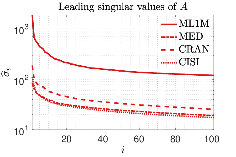
Figure 1: Leading k=100k=100 singular values.
Refer to caption
Refer to caption
Refer to caption
Refer to caption
Refer to caption
Refer to caption
Refer to caption
Refer to caption
Figure 2: Approximation of the leading k=50k=50 singular triplets for the single update case. From left to right: MED, CRAN, CISI, and 1M.

Table 2 lists the test matrices considered throughout our experiments along with their dimensions and source from which they were retrieved. The first three matrices come from LSI applications and represent term-document matrices, while the last matrix comes from recommender systems and represents a user-item rating matrix. The k=100k=100 leading singular values of each matrix listed in Table 2 are plotted in Figure 1.

Throughout this section we focus on accuracy and will be reporting: a) the relative error in the approximation of the kk leading singular values of AA, and b) the norm of the residual A​v^(i)−σ^i​u^(i)A\widehat{v}^{(i)}-\widehat{\sigma}_{i}\widehat{u}^{(i)}, scaled by σ^i\widehat{\sigma}_{i}. The scalar λ\lambda is set as λ=1.01​σ^12\lambda=1.01\widehat{\sigma}_{1}^{2} where the latter singular value is approximated by a few iterations of Lanczos bidiagonalization.

5.1 Single update.

In this section we consider the approximation of the k=50k=50 leading singular triplets of A=(BE)A=\begin{pmatrix}B\\ E\\ \end{pmatrix} where B=A(1:⌈m/2⌉,:)B=A(1:\lceil m/2\rceil,:), i.e., the size of matrices BB and EE is about half the size of AA. We run Algorithm 1 and set ZZ as in Propositions 4.3 and 4.5. For the enhanced matrix ZZ, the matrix Xλ,rX_{\lambda,r} is computed by randomized SVD where r=kr=k and the number of columns in matrix RR is equal to 2​k2k (recall the discussion in Section 4.3). The associated linear system with 2​k2k right-hand sides is solved by block Conjugate Gradient.

Figure 2 plots the relative error and residual norm in the approximation of the k=50k=50 leading singular triplets of AA. As expected, enhancing the projection matrix ZZ by Xλ,rX_{\lambda,r} leads to higher accuracy. This is especially true for the approximation of those singular triplets with corresponding singular values σ^i≈λ\widehat{\sigma}_{i}\approx\lambda.

In all of our experiments, the worst-case (maximum) relative error and residual norm was achieved in the approximation of the singular triplet (σ^50,u^(50),v^(50))(\hat{\sigma}_{50},\hat{u}^{(50)},\hat{v}^{(50)}). Table 3 lists the relative error and residual norm associated with the approximation of the singular triplet (σ^50,u^(50),v^(50))(\hat{\sigma}_{50},\hat{u}^{(50)},\hat{v}^{(50)}) as rr varies from ten to fifty in increments of ten. As a reference, we list the same quantity for the case Z=(UkIs)Z=\begin{pmatrix}U_{k}&\\ &I_{s}\\ \end{pmatrix}. As expected, enhancing the projection matrix ZZ by Xλ,rX_{\lambda,r} leads to higher accuracy, especially for higher values of rr.

Table 3: Relative error and residual norm associated with the approximation of the singular triplet (σ^50,u^(50),v^(50))(\widehat{\sigma}_{50},\widehat{u}^{(50)},\widehat{v}^{(50)}).
MED CRAN CISI ML1M
rr err. res. err. res. err. res. err. res.
Z=(UkXλ,rIs)Z=\begin{pmatrix}U_{k}&X_{\lambda,r}&\\ &&I_{s}\\ \end{pmatrix}    r=10r=10 0.036 0.234 0.026 0.176 0.025 0.214 0.031 0.156
r=20r=20 0.031 0.184 0.021 0.155 0.023 0.189 0.012 0.143
r=30r=30 0.021 0.114 0.017 0.134 0.017 0.161 0.008 0.121
r=40r=40 0.009 0.091 0.013 0.111 0.012 0.134 0.005 0.112
r=50r=50 0.004 0.053 0.007 0.098 0.007 0.081 0.003 0.076
Z=(UkIs)Z=\begin{pmatrix}U_{k}&\\ &I_{s}\\ \end{pmatrix}    N/A 0.045 0.269 0.045 0.199 0.287 0.250 0.041 0.173
Refer to caption
Refer to caption
Refer to caption
Refer to caption
Refer to caption
Refer to caption
Refer to caption
Refer to caption
Figure 3: Relative error in the approximation of the k=50k=50 leading singular values of AA for the multiple updates case. From left to right: MED, CRAN, CISI, and 1M.
Refer to caption
Refer to caption
Refer to caption
Refer to caption
Refer to caption
Refer to caption
Refer to caption
Refer to caption
Figure 4: Residual norm of the approximation of the k=50k=50 leading singular triplets of AA for the multiple updates case. From left to right: MED, CRAN, CISI, and 1M.

5.2 Sequence of updates.

In this experiment the rows of matrix EE are now added in batches, i.e., we first approximate the kk leading singular triplets of matrix A(0)=(BA(⌈m/2⌉+1:⌈m/2⌉+t,:))A^{(0)}=\begin{pmatrix}B\\ A(\lceil m/2\rceil+1:\lceil m/2\rceil+t,:)\\ \end{pmatrix}, then of matrix A(1)=(A(0)A(⌈m/2⌉+t+1:⌈m/2⌉+2t,:))A^{(1)}=\begin{pmatrix}A^{(0)}\\ A(\lceil m/2\rceil+t+1:\lceil m/2\rceil+2t,:)\\ \end{pmatrix}, etc. Here, t=⌈m/2⌉/ϕt=\lceil m/2\rceil/\phi denotes the step-size and ϕ∈ℤ∗\phi\in\mathbb{Z}^{*} denotes the total number of updates. Note that after the first update, the matrices UkU_{k} and VkV_{k} no longer denote the exact kk leading left and right singular vectors of the B≡A(j−1)B\equiv A^{(j-1)} submatrix of matrix A(j)A^{(j)}. We set ϕ=12\phi=12 and plot the accuracy achieved after one, six, and twelve updates, in Figures 3 and 4. Notice that enhancing ZZ by Xλ,rX_{\lambda,r} leads to similar accuracy for all updates, while in the opposite case accuracy deteriorates as the updates accumulate. On a separate note, the accuracy of the kk leading singular triplets of AA is higher when matrix EE is added to BB in batches rather than in a single update as in the previous section.

Table 4: Maximum relative error and residual norm of the approximation of the kk leading singular triplets of AA for the multiple updates case as kk varies.
MED CRAN CISI ML1M
Method err. res. err. res. err. res. err. res.
k=10k=10    [31] 0.046 0.172 0.043 0.192 0.054 0.274 0.002 0.058
Alg. 1 0.001 0.045 0.008 0.090 0.002 0.054 3.0​𝚎3.0\mathtt{e}-5 0.007
k=20k=20    [31] 0.067 0.212 0.064 0.255 0.075 0.224 0.022 0.131
Alg. 1 0.004 0.073 0.005 0.076 0.003 0.053 0.002 0.040
k=30k=30    [31] 0.076 0.384 0.060 0.290 0.084 0.330 0.023 0.123
Alg. 1 0.006 0.067 0.008 0.088 0.004 0.070 0.001 0.041

Table 4 lists relative error and residual norm associated with the approximation of the singular triplet (σ^50,u^(50),v^(50))(\widehat{\sigma}_{50},\widehat{u}^{(50)},\widehat{v}^{(50)}) by Algorithm 1 and the method in [31]. The number of sought singular triplets kk was varied from ten to thirty. Comparisons against the method in [28] were also performed but not reported since the latter was always less accurate than [31]. Overall, Algorithm 1 provided higher accuracy, especially for those singular triplets whose corresponding singular value was closer to λ\lambda.

6 Conclusion

This paper presented an algorithm to update the rank-kk truncated SVD of evolving matrices. The proposed algorithm undertakes a projection viewpoint and aims on building a pair of subspaces which approximate the linear span of the kk leading singular vectors of the updated matrix. Two different options to set these subspaces were considered. Experiments performed on matrices stemming from applications in LSI and recommender systems verified the effectiveness of the proposed scheme in terms of accuracy.

References

  • [1] http://web.eecs.utk.edu/research/lsi/.
  • [2] J. Baglama and L. Reichel, Augmented implicitly restarted Lanczos bidiagonalization methods, SIAM Journal on Scientific Computing, 27 (2005), pp. 19–42.
  • [3] M. W. Berry, S. T. Dumais, and G. W. O’Brien, Using linear algebra for intelligent information retrieval, SIAM Review, 37 (1995), pp. 573–595.
  • [4] M. Brand, Fast online SVD revisions for lightweight recommender systems, in Proceedings of the 2003 SIAM International Conference on Data Mining, SIAM, 2003, pp. 37–46.
  • [5] K. L. Clarkson and D. P. Woodruff, Numerical linear algebra in the streaming model, in Proceedings of the forty-first annual ACM symposium on Theory of computing, 2009, pp. 205–214.
  • [6] P. Cremonesi, Y. Koren, and R. Turrin, Performance of recommender algorithms on top-n recommendation tasks, in Proceedings of the fourth ACM conference on Recommender systems, 2010, pp. 39–46.
  • [7] S. Deerwester, S. T. Dumais, G. W. Furnas, T. K. Landauer, and R. Harshman, Indexing by latent semantic analysis, Journal of the American society for information science, 41 (1990), pp. 391–407.
  • [8] G. Golub and W. Kahan, Calculating the singular values and pseudo-inverse of a matrix, Journal of the Society for Industrial and Applied Mathematics, Series B: Numerical Analysis, 2 (1965), pp. 205–224.
  • [9] M. Gu, Stanley, and S. C. Eisenstat, A stable and fast algorithm for updating the singular value decomposition, tech. rep., 1994.
  • [10] N. Halko, P.-G. Martinsson, and J. A. Tropp, Finding structure with randomness: Probabilistic algorithms for constructing approximate matrix decompositions, SIAM Review, 53 (2011), pp. 217–288.
  • [11] F. M. Harper and J. A. Konstan, The movielens datasets: History and context, ACM transactions on interactive intelligent systems, 5 (2015), pp. 1–19.
  • [12] V. Hernandez, J. E. Roman, and V. Vidal, SLEPc: A scalable and flexible toolkit for the solution of eigenvalue problems, ACM Transactions on Mathematical Software (TOMS), 31 (2005), pp. 351–362.
  • [13] L. Horesh, A. R. Conn, E. A. Jimenez, and G. M. van Essen, Reduced space dynamics-based geo-statistical prior sampling for uncertainty quantification of end goal decisions, in Numerical Analysis and Optimization, Springer, 2015, pp. 191–221.
  • [14] Z. Jia and G. Stewart, An analysis of the Rayleigh-Ritz method for approximating eigenspaces, Mathematics of computation, 70 (2001), pp. 637–647.
  • [15] V. Kalantzis, C. Bekas, A. Curioni, and E. Gallopoulos, Accelerating data uncertainty quantification by solving linear systems with multiple right-hand sides, Numerical Algorithms, 62 (2013), pp. 637–653.
  • [16] V. Kalantzis, A. C. I. Malossi, C. Bekas, A. Curioni, E. Gallopoulos, and Y. Saad, A scalable iterative dense linear system solver for multiple right-hand sides in data analytics, Parallel Computing, 74 (2018), pp. 136–153.
  • [17] M. Moonen, P. Van Dooren, and J. Vandewalle, A singular value decomposition updating algorithm for subspace tracking, SIAM Journal on Matrix Analysis and Applications, 13 (1992), pp. 1015–1038.
  • [18] Y. Nakatsukasa, Accuracy of singular vectors obtained by projection-based SVD methods, BIT Numerical Mathematics, 57 (2017), pp. 1137–1152.
  • [19] A. N. Nikolakopoulos, V. Kalantzis, E. Gallopoulos, and J. D. Garofalakis, Eigenrec: generalizing PureSVD for effective and efficient top-N recommendations, Knowledge and Information Systems, 58 (2019), pp. 59–81.
  • [20] D. P. O’Leary, The block Conjugate Gradient algorithm and related methods, Linear Algebra and its Applications, 29 (1980), pp. 293–322.
  • [21] Y. Saad, Numerical methods for large eigenvalue problems: revised edition, SIAM, 2011.
  • [22] Y. Saad, M. Yeung, J. Erhel, and F. Guyomarc’h, A deflated version of the Conjugate Gradient algorithm, SIAM Journal on Scientific Computing, 21 (2000), pp. 1909–1926.
  • [23] B. Sarwar, G. Karypis, J. Konstan, and J. Riedl, Incremental singular value decomposition algorithms for highly scalable recommender systems, in Fifth international conference on computer and information science, vol. 1, Citeseer, 2002, pp. 27–8.
  • [24] A. Stathopoulos and K. Orginos, Computing and deflating eigenvalues while solving multiple right-hand side linear systems with an application to quantum chromodynamics, SIAM Journal on Scientific Computing, 32 (2010), pp. 439–462.
  • [25] S. Ubaru, A. Mazumdar, and Y. Saad, Low rank approximation using error correcting coding matrices, in International Conference on Machine Learning, 2015, pp. 702–710.
  • [26] S. Ubaru and Y. Saad, Sampling and multilevel coarsening algorithms for fast matrix approximations, Numerical Linear Algebra with Applications, 26 (2019), p. e2234.
  • [27] S. Ubaru, A.-K. Seghouane, and Y. Saad, Find the dimension that counts: Fast dimension estimation and Krylov PCA, in Proceedings of the 2019 SIAM International Conference on Data Mining, SIAM, 2019, pp. 720–728.
  • [28] E. Vecharynski and Y. Saad, Fast updating algorithms for latent semantic indexing, SIAM Journal on Matrix Analysis and Applications, 35 (2014), pp. 1105–1131.
  • [29] L. Wu and A. Stathopoulos, A preconditioned hybrid SVD method for accurately computing singular triplets of large matrices, SIAM Journal on Scientific Computing, 37 (2015), pp. S365–S388.
  • [30] I. Yamazaki, S. Tomov, and J. Dongarra, Sampling algorithms to update truncated SVD, in 2017 IEEE International Conference on Big Data, IEEE, 2017, pp. 817–826.
  • [31] H. Zha and H. D. Simon, On updating problems in latent semantic indexing, SIAM Journal on Scientific Computing, 21 (1999), pp. 782–791.
  • [32] H. Zha and Z. Zhang, Matrices with low-rank-plus-shift structure: partial SVD and latent semantic indexing, SIAM Journal on Matrix Analysis and Applications, 21 (2000), pp. 522–536.

Supplementary Material

Asymptotic complexity

The asymptotic complexity analysis of the method in [31] is as follows. We need O⁡(n​s2+n​s​k)O\left(ns^{2}+nsk\right) FLOPs to form (Is−Vk​VkH)​EH(I_{s}-V_{k}V_{k}^{H})E^{H} and compute its QR decomposition. The SVD of the matrix ZH​A​WZ^{H}AW requires O⁡((k+s)3)O\left((k+s)^{3}\right) FLOPs. Finally, the cost to form the approximation of matrices U^k\widehat{U}_{k} and V^k\widehat{V}_{k} is equal to O⁡(k2​(m+n)+n​s​k)O\left(k^{2}(m+n)+nsk\right) FLOPs.

The asymptotic complexity analysis for the “SV” variant of the method in [28] is as follows. We need O⁡((𝚗𝚗𝚣⁡(E)+n​k)​δ1+(n+s)​δ12)O\left((\mathtt{nnz}(E)+nk)\delta_{1}+(n+s)\delta_{1}^{2}\right) FLOPs to approximate the rr leading singular triplets of (Is−Vk​VkH)​EH(I_{s}-V_{k}V_{k}^{H})E^{H}, where δ1∈ℤ∗\delta_{1}\in\mathbb{Z}^{*} is greater than or equal to rr (i.e., δ1\delta_{1} is the number of Lanczos bidiagonalization steps). The cost to form and compute the SVD of the matrix ZH​A​WZ^{H}AW is equal to (k+s)​(k+r)2+𝚗𝚗𝚣⁡(E)​k+r​s(k+s)(k+r)^{2}+\mathtt{nnz}(E)k+rs where the first term stands for the actual SVD and the rest of the terms stand for the formation of the matrix ZH​A​WZ^{H}AW. Finally, the cost to form the approximation of matrices U^k\widehat{U}_{k} and V^k\widehat{V}_{k} is equal to O⁡(k2​(m+n)+n​r​k)O\left(k^{2}(m+n)+nrk\right) FLOPs.

The asymptotic complexity analysis of Algorithm 1 is as follows. First, notice that Algorithm 1 requires no effort to build WW. For the case where ZZ is set as in Proposition 4.3, termed as “Alg. 1 (a)”, we also need no FLOPs to build ZZ. The cost to solve the projected problem by unrestarted Lanczos is then equal to O⁡((𝚗𝚗𝚣⁡(E)+n​k)​δ2+(k+s)​δ22)O\left((\mathtt{nnz}(E)+nk)\delta_{2}+(k+s)\delta_{2}^{2}\right) FLOPs, where δ2∈ℤ∗\delta_{2}\in\mathbb{Z}^{*} is greater than or equal to kk (i.e., δ2\delta_{2} is the number of unrestarted Lanczos steps). Finally, the cost to form the approximation of matrices U^k\widehat{U}_{k} and V^k\widehat{V}_{k} is equal to O⁡(k2​m+(𝚗𝚗𝚣⁡(A)+n)​k)O\left(k^{2}m+(\mathtt{nnz}(A)+n)k\right) FLOPs. For the case where ZZ is set as in Proposition 4.5, termed as “Alg. 1 (b)”, we need

χ=O⁡(𝚗𝚗𝚣⁡(A)​δ3+m​δ32)\chi=O\left(\mathtt{nnz}(A)\delta_{3}+m\delta_{3}^{2}\right)

FLOPs to build Xλ,rX_{\lambda,r}, where δ3∈ℤ∗\delta_{3}\in\mathbb{Z}^{*} is greater than or equal to kk (i.e., δ3\delta_{3} is either the number of Lanczos bidiagonalization steps or the number of columns of matrix RR in randomized SVD).

Table 5: Detailed asymptotic complexity of Algorithm 1 and the schemes in [31] and [28]. All δ\delta variables are replaced by kk.
Scheme Building ZZ Building WW Solving the projected problem Other
[31] - n​s2+n​s​kns^{2}+nsk (k+s)3(k+s)^{3} k2​(m+n)+n​s​kk^{2}(m+n)+nsk
[28] - (𝚗𝚗𝚣⁡(E)+n​k)​k+(n+s)​k2(\mathtt{nnz}(E)+nk)k+(n+s)k^{2} (k+s)​(k+r)2+𝚗𝚗𝚣⁡(E)​k+r​s(k+s)(k+r)^{2}+\mathtt{nnz}(E)k+rs k2​(m+n)+n​r​kk^{2}(m+n)+nrk
Alg. 1 (a) - - (𝚗𝚗𝚣⁡(E)+n​k)​k+(k+s)​k2(\mathtt{nnz}(E)+nk)k+(k+s)k^{2} k2​m+(𝚗𝚗𝚣⁡(A)+n)​kk^{2}m+(\mathtt{nnz}(A)+n)k
Alg. 1 (b) χ\chi - (𝚗𝚗𝚣⁡(E)+(n+r)​k)​k+(k+r+s)​k2(\mathtt{nnz}(E)+(n+r)k)k+(k+r+s)k^{2} k2​m+(𝚗𝚗𝚣⁡(A)+n)​kk^{2}m+(\mathtt{nnz}(A)+n)k

The above discussion is summarized in Table 5 where we list the asymptotic complexity of Algorithm 1 and the schemes in [31] and [28]. The complexities of the latter two schemes were also verified by adjusting the complexity analysis from [28]. To allow for a practical comparison, we replaced all δ\delta variables with kk since in practice these variables are equal to at most a small integer multiple of kk.

Consider now a comparison between Algorithm 1 (a) and the method in [31]. For all practical purposes, these two schemes return identical approximations to AkA_{k}. Nonetheless, Algorithm 1 (a) requires no effort to build WW. Moreover, the cost to solve the projected problem is linear with respect to ss and cubic with respect to kk, instead of cubic with respect to the sum s+ks+k in [31]. The only scenario where Algorithm 1 can be potentially more expensive than [31] is when matrix AA is exceptionally dense, and both kk and ss are very small. Similar observations can be made for the relation between Algorithm 1 (b) and the methods in [28], although the comparison is more involved.

Proofs

Proof of Proposition 4.1

The scalar-vector pair (σ^i2,u^(i))(\widehat{\sigma}_{i}^{2},\widehat{u}^{(i)}) satisfies the equation (A​AH−σ^i2​Im+s)​u^(i)=0(AA^{H}-\widehat{\sigma}_{i}^{2}I_{m+s})\widehat{u}^{(i)}=0. If we partition the ii’th left singular vector as

u^(i)=(f^(i)y^(i)),\widehat{u}^{(i)}=\begin{pmatrix}\widehat{f}^{(i)}\\[3.00003pt] \widehat{y}^{(i)}\\[3.00003pt] \end{pmatrix},

we can write

(B​BH−σ^i2​ImB​EHE​BHE​EH−σ^i2​Is)​(f^(i)y^(i))=0.\begin{pmatrix}BB^{H}-\widehat{\sigma}_{i}^{2}I_{m}&BE^{H}\\[3.00003pt] EB^{H}&EE^{H}-\widehat{\sigma}_{i}^{2}I_{s}\\[3.00003pt] \end{pmatrix}\begin{pmatrix}\widehat{f}^{(i)}\\[3.00003pt] \widehat{y}^{(i)}\\[3.00003pt] \end{pmatrix}=0.

The leading mm rows satisfy (B​BH−σ^i2​Im)​f^(i)=−B​EH​y^(i)(BB^{H}-\widehat{\sigma}_{i}^{2}I_{m})\widehat{f}^{(i)}=-BE^{H}\widehat{y}^{(i)}. Plugging the expression of f^(i)\widehat{f}^{(i)} in the second block of rows and considering the full SVD B=U​Σ​VHB=U\Sigma V^{H} leads to

0\displaystyle 0 =[E​EH−E​BH​(B​BH−σ^i2​Im)−1​B​EH−σ^i2​Is]​y^(i)\displaystyle=\left[EE^{H}-EB^{H}(BB^{H}-\widehat{\sigma}_{i}^{2}I_{m})^{-1}BE^{H}-\widehat{\sigma}_{i}^{2}I_{s}\right]\widehat{y}^{(i)}
=[E⁡(Is−BH​(B​BH−σ^i2​Im)−1​B)​EH−σ^i2​Is]​y^(i)\displaystyle=\left[E(I_{s}-B^{H}(BB^{H}-\widehat{\sigma}_{i}^{2}I_{m})^{-1}B)E^{H}-\widehat{\sigma}_{i}^{2}I_{s}\right]\widehat{y}^{(i)}
=[E⁡(V​VH+V​ΣT​(σ^i2​Im−Σ​ΣT)−1​Σ​VH)​EH−σ^i2​Is]​y^(i)\displaystyle=\left[E(VV^{H}+V\Sigma^{T}(\widehat{\sigma}_{i}^{2}I_{m}-\Sigma\Sigma^{T})^{-1}\Sigma V^{H})E^{H}-\widehat{\sigma}_{i}^{2}I_{s}\right]\widehat{y}^{(i)}
=[E​V​(In+ΣT​(σ^i2​Im−Σ​ΣT)−1​Σ)​VH​EH−σ^i2​Is]​y^(i).\displaystyle=\left[EV(I_{n}+\Sigma^{T}\left(\widehat{\sigma}_{i}^{2}I_{m}-\Sigma\Sigma^{T}\right)^{-1}\Sigma)V^{H}E^{H}-\widehat{\sigma}_{i}^{2}I_{s}\right]\widehat{y}^{(i)}.

The proof concludes by noticing that

In+ΣT​(σ^i2​Im−Σ​ΣT)−1​Σ=(1+σ12σ^i2−σ12⋱1+σn2σ^i2−σn2)=(σ^i2σ^i2−σ12⋱σ^i2σ^i2−σn2),I_{n}+\Sigma^{T}\left(\widehat{\sigma}_{i}^{2}I_{m}-\Sigma\Sigma^{T}\right)^{-1}\Sigma=\begin{pmatrix}1+\dfrac{\sigma_{1}^{2}}{\widehat{\sigma}_{i}^{2}-\sigma_{1}^{2}}&&\\[3.00003pt] &\ddots&\\[3.00003pt] &&1+\dfrac{\sigma_{n}^{2}}{\widehat{\sigma}_{i}^{2}-\sigma_{n}^{2}}\\[3.00003pt] \end{pmatrix}=\begin{pmatrix}\dfrac{\widehat{\sigma}_{i}^{2}}{\widehat{\sigma}_{i}^{2}-\sigma_{1}^{2}}&&\\[3.00003pt] &\ddots&\\[3.00003pt] &&\dfrac{\widehat{\sigma}_{i}^{2}}{\widehat{\sigma}_{i}^{2}-\sigma_{n}^{2}}\\[3.00003pt] \end{pmatrix},

where for the case m<nm<n, we have σj=0\sigma_{j}=0 for any j=m+1,…,nj=m+1,\ldots,n. In case σ^i=σj\widehat{\sigma}_{i}=\sigma_{j}, the Moore-Penrose pseudoinverse (B​BH−σ^i2​Im)†(BB^{H}-\widehat{\sigma}_{i}^{2}I_{m})^{\dagger} is considered instead.

Proof of Proposition 4.2

Since the left singular vectors of BB span ℝm\mathbb{R}^{m}, we can write

B​EH​y^(i)=∑j=1mσj​u(j)​(E​v(j))H​y^(i).BE^{H}\widehat{y}^{(i)}=\sum\limits_{j=1}^{m}\sigma_{j}u^{(j)}\left(Ev^{(j)}\right)^{H}\widehat{y}^{(i)}.

The proof concludes by noticing that the top m×1m\times 1 part of u^(i)\widehat{u}^{(i)} can be written as

f^(i)\displaystyle\widehat{f}^{(i)} =−(B​BH−σ^i2​Im)−1​B​EH​y^(i)\displaystyle=-(BB^{H}-\widehat{\sigma}_{i}^{2}I_{m})^{-1}BE^{H}\widehat{y}^{(i)}
=−U​(Σ​ΣT−σ^i2​Im)−1​Σ​(E​V)H​y^(i)\displaystyle=-U(\Sigma\Sigma^{T}-\widehat{\sigma}_{i}^{2}I_{m})^{-1}\Sigma\left(EV\right)^{H}\widehat{y}^{(i)}
=−∑j=1𝚖𝚒𝚗⁡(m,n)u(j)σjσj2−σ^i2(Ev(j))Hy^(i)\displaystyle=-\sum\limits_{j=1}^{\mathtt{min}(m,n)}u^{(j)}\dfrac{\sigma_{j}}{\sigma_{j}^{2}-\widehat{\sigma}_{i}^{2}}\left(Ev^{(j)}\right)^{H}\widehat{y}^{(i)}
=∑j=1𝚖𝚒𝚗⁡(m,n)u(j)​χj,i.\displaystyle=\sum\limits_{j=1}^{\mathtt{min}(m,n)}u^{(j)}\chi_{j,i}.

Proof of Proposition 4.3

We have

𝚖𝚒𝚗z∈𝚛𝚊𝚗𝚐𝚎⁡(Z)​‖u^(i)−z‖\displaystyle\mathtt{min}_{z\in\mathtt{range}(Z)}\|\widehat{u}^{(i)}-z\| ≤‖(u(k+1),…,u(𝚖𝚒𝚗⁡(m,n)))​(χk+1,iχ𝚖𝚒𝚗⁡(m,n),i)‖\displaystyle\leq\left\lVert\begin{pmatrix}u^{(k+1)},\ldots,u^{(\mathtt{min}(m,n))}\\[3.00003pt] \\[3.00003pt] \end{pmatrix}\begin{pmatrix}\chi_{k+1,i}\\[3.00003pt] \vdots\\[3.00003pt] \chi_{\mathtt{min}(m,n),i}\\[3.00003pt] \end{pmatrix}\right\rVert
=‖(0k,kσk+1σk+12−σ^i2⋱σ𝚖𝚒𝚗⁡(m,n)σ𝚖𝚒𝚗⁡(m,n)2−σ^i2)​VH​EH​y^(i)‖\displaystyle=\left\lVert\left(\begin{smallmatrix}\scalebox{2}{$0$}_{k,k}&&&&\\ &&\dfrac{\sigma_{k+1}}{\sigma_{k+1}^{2}-\widehat{\sigma}_{i}^{2}}&&\\ &&&\ddots&\\ &&&&\dfrac{\sigma_{\mathtt{min}(m,n)}}{\sigma_{\mathtt{min}(m,n)}^{2}-\widehat{\sigma}_{i}^{2}}\\ \end{smallmatrix}\right)V^{H}E^{H}\hat{y}^{(i)}\right\rVert
≤𝚖𝚊𝚡​{|σjσj2−σ^i2|}j=k+1,…,𝚖𝚒𝚗⁡(m,n)​‖EH​y^(i)‖.\displaystyle\leq\mathtt{max}\left\{\left|\dfrac{\sigma_{j}}{\sigma_{j}^{2}-\widehat{\sigma}_{i}^{2}}\right|\right\}_{j=k+1,\ldots,\mathtt{min}(m,n)}\left\lVert E^{H}\widehat{y}^{(i)}\right\rVert.

The proof follows by noticing that due to Cauchy’s interlacing theorem we have σk+12≤σ^i2,i=1,…,k\sigma_{k+1}^{2}\leq\widehat{\sigma}_{i}^{2},\ i=1,\ldots,k, and thus |σk+1σk+12−σ^i2|≥⋯≥|σ𝚖𝚒𝚗⁡(m,n)σ𝚖𝚒𝚗⁡(m,n)2−σ^i2|.\left|\dfrac{\sigma_{k+1}}{\sigma_{k+1}^{2}-\widehat{\sigma}_{i}^{2}}\right|\geq\cdots\geq\left|\dfrac{\sigma_{\mathtt{min}(m,n)}}{\sigma_{\mathtt{min}(m,n)}^{2}-\widehat{\sigma}_{i}^{2}}\right|.

Proof of Lemma 4.1

We can write

B⁡(λ)\displaystyle B(\lambda) =(I−Uk​UkH)​U​(σ12−λ⋱σm2−λ)−1​UH\displaystyle=\left(I-U_{k}U_{k}^{H}\right)U\left(\begin{smallmatrix}\sigma_{1}^{2}-\lambda&&\\ &\ddots&\\ &&\sigma_{m}^{2}-\lambda\end{smallmatrix}\right)^{-1}U^{H}
=U⁡(0k,k1σk+12−λ⋱1σm2−λ)​UH,\displaystyle=U\left(\begin{smallmatrix}\scalebox{2}{$0$}_{k,k}&&&&\\ &&\dfrac{1}{\sigma_{k+1}^{2}-\lambda}&&\\ &&&\ddots&\\ &&&&\dfrac{1}{\sigma_{m}^{2}-\lambda}\\ \end{smallmatrix}\right)U^{H},

where σj=0\sigma_{j}=0 for any j>𝚖𝚒𝚗⁡(m,n)j>\mathtt{min}(m,n). Let us now define the scalar γj,i=σ^i2−λσj2−λ\gamma_{j,i}=\dfrac{\widehat{\sigma}_{i}^{2}-\lambda}{\sigma_{j}^{2}-\lambda}. Then,

B⁡(λ)​[(σ^i2−λ)​B​(λ)]ρ=U​(0k,kγk+1,iρσk+12−λ⋱γm,iρσm2−λ)​UH.B(\lambda)\left[(\widehat{\sigma}_{i}^{2}-\lambda)B(\lambda)\right]^{\rho}=U\begin{pmatrix}\scalebox{2}{$0$}_{k,k}&&&\\[3.00003pt] &\dfrac{\gamma_{k+1,i}^{\rho}}{\sigma_{k+1}^{2}-\lambda}&&\\[3.00003pt] &&\ddots&\\[3.00003pt] &&&\dfrac{\gamma_{m,i}^{\rho}}{\sigma_{m}^{2}-\lambda}\\[3.00003pt] \end{pmatrix}U^{H}.

Accounting for all powers p=0,1,2,…p=0,1,2,\ldots, gives

B⁡(λ)​∑ρ=0∞[(σ^i2−λ)​B​(λ)]ρ=U​(0k,k∑ρ=0∞γk+1,iρσk+12−λ⋱∑ρ=0∞γm,iρσm2−λ)​UH.B(\lambda)\sum_{\rho=0}^{\infty}\left[(\widehat{\sigma}_{i}^{2}-\lambda)B(\lambda)\right]^{\rho}=U\begin{pmatrix}\scalebox{2}{$0$}_{k,k}&&&\\[2.77501pt] &\dfrac{\sum_{\rho=0}^{\infty}\gamma_{k+1,i}^{\rho}}{\sigma_{k+1}^{2}-\lambda}&&\\[2.77501pt] &&\ddots&\\[2.77501pt] &&&\dfrac{\sum_{\rho=0}^{\infty}\gamma_{m,i}^{\rho}}{\sigma_{m}^{2}-\lambda}\\[2.77501pt] \end{pmatrix}U^{H}.

Since λ>σ^k2≥σk2\lambda>\widehat{\sigma}_{k}^{2}\geq\sigma_{k}^{2}, it follows that for any j>kj>k we have |γj,i|<1|\gamma_{j,i}|<1. Therefore, the geometric series converges and ∑ρ=0∞γj,iρ=11−γj,i=σj2−λσj2−σ^i2\sum_{\rho=0}^{\infty}\gamma_{j,i}^{\rho}=\dfrac{1}{1-\gamma_{j,i}}=\dfrac{\sigma_{j}^{2}-\lambda}{\sigma_{j}^{2}-\widehat{\sigma}_{i}^{2}}. It follows that 1σj2−λ​∑ρ=0∞γjρ=1σj2−σ^i2\dfrac{1}{\sigma_{j}^{2}-\lambda}\sum_{\rho=0}^{\infty}\gamma_{j}^{\rho}=\dfrac{1}{\sigma_{j}^{2}-\widehat{\sigma}_{i}^{2}}.

We finally have

B⁡(λ)​∑ρ=0∞[(σ^i2−λ)​B​(λ)]ρ\displaystyle B(\lambda)\sum_{\rho=0}^{\infty}\left[(\widehat{\sigma}_{i}^{2}-\lambda)B(\lambda)\right]^{\rho} =U​(0k,k1σk+12−σ^i2⋱1σm2−σ^i2)​UH\displaystyle=U\begin{pmatrix}\scalebox{2}{$0$}_{k,k}&&&&\\[3.00003pt] &\dfrac{1}{\sigma_{k+1}^{2}-\widehat{\sigma}_{i}^{2}}&&\\[3.00003pt] &&\ddots&\\[3.00003pt] &&&\dfrac{1}{\sigma_{m}^{2}-\widehat{\sigma}_{i}^{2}}\\[3.00003pt] \end{pmatrix}U^{H}
=(I−Uk​UkH)​B​(σ^i2).\displaystyle=\left(I-U_{k}U_{k}^{H}\right)B(\widehat{\sigma}_{i}^{2}).

This concludes the proof.

Proof of Proposition 4.4

First, notice that

(B​BH−σ^i2​Im)−1=Uk​UkH​(B​BH−σ^i2​Im)−1+(Im−Uk​UkH)​(B​BH−σ^i2​Im)−1.(BB^{H}-\widehat{\sigma}_{i}^{2}I_{m})^{-1}=U_{k}U_{k}^{H}(BB^{H}-\widehat{\sigma}_{i}^{2}I_{m})^{-1}+(I_{m}-U_{k}U_{k}^{H})(BB^{H}-\widehat{\sigma}_{i}^{2}I_{m})^{-1}.

Therefore, we can write

(B​BH−σ^i2​Im)−1​B​EH​y^(i)=Uk​(Σk2−σ^i2​Ik)−1​Σk​(E​Vk)H​y^(i)+(Im−Uk​UkH)​(B​BH−σ^i2​Im)−1​B​EH​y^(i).(BB^{H}-\widehat{\sigma}_{i}^{2}I_{m})^{-1}BE^{H}\widehat{y}^{(i)}=U_{k}(\Sigma_{k}^{2}-\widehat{\sigma}_{i}^{2}I_{k})^{-1}\Sigma_{k}(EV_{k})^{H}\widehat{y}^{(i)}+(I_{m}-U_{k}U_{k}^{H})(BB^{H}-\widehat{\sigma}_{i}^{2}I_{m})^{-1}BE^{H}\widehat{y}^{(i)}.

The left singular vector u^(i)\widehat{u}^{(i)} can be then expressed as

u^(i)\displaystyle\widehat{u}^{(i)} =\displaystyle= (−(B​BH−σ^i2​Im)−1​B​EHIs)​y^(i)\displaystyle\begin{pmatrix}-(BB^{H}-\widehat{\sigma}_{i}^{2}I_{m})^{-1}BE^{H}\\[3.00003pt] I_{s}\\[3.00003pt] \end{pmatrix}\widehat{y}^{(i)}
=\displaystyle= (u(1),…,u(k)Is)​(χ1,iχk,iy^(i))−(B⁡(σ^i2)​B​EH​y^(i)).\displaystyle\begin{pmatrix}u^{(1)},\ldots,u^{(k)}&\\[3.00003pt] &I_{s}\\[3.00003pt] \end{pmatrix}\begin{pmatrix}\chi_{1,i}\\[3.00003pt] \vdots\\[3.00003pt] \chi_{k,i}\\[3.00003pt] \widehat{y}^{(i)}\\[3.00003pt] \end{pmatrix}-\begin{pmatrix}B(\widehat{\sigma}_{i}^{2})BE^{H}\widehat{y}^{(i)}\\[3.00003pt] \\[3.00003pt] \end{pmatrix}.

The proof concludes by noticing that by Lemma 4.1 we have B⁡(σ^i2)=B⁡(λ)​∑ρ=0∞[(σ^i2−λ)​B​(λ)]ρB(\widehat{\sigma}_{i}^{2})=B(\lambda)\sum\limits_{\rho=0}^{\infty}\left[(\widehat{\sigma}_{i}^{2}-\lambda)B(\lambda)\right]^{\rho}.

Proof of Proposition 4.5

The proof exploits the formula

(B⁡(σ^i2)−B⁡(λ))​B​EH=(I−Uk​UkH)​U​[(Σ​ΣT−σ^i2​Im)−1−(Σ​ΣT−λ​Im)−1]​UH​U​Σ​VH​EH.(B(\widehat{\sigma}_{i}^{2})-B(\lambda))BE^{H}=(I-U_{k}U_{k}^{H})U\left[(\Sigma\Sigma^{T}-\widehat{\sigma}_{i}^{2}I_{m})^{-1}-(\Sigma\Sigma^{T}-\lambda I_{m})^{-1}\right]U^{H}U\Sigma V^{H}E^{H}.

It follows

𝚖𝚒𝚗z∈𝚛𝚊𝚗𝚐𝚎⁡(Z)​‖u^(i)−z‖\displaystyle\mathtt{min}_{z\in\mathtt{range}(Z)}\|\widehat{u}^{(i)}-z\| ≤\displaystyle\leq ‖([B⁡(σ^i2)−B⁡(λ)]​B​EH​y^(i))‖\displaystyle\left\lVert\begin{pmatrix}\left[B(\widehat{\sigma}_{i}^{2})-B(\lambda)\right]BE^{H}\widehat{y}^{(i)}\\[3.00003pt] \\[3.00003pt] \end{pmatrix}\right\rVert
≤\displaystyle\leq ‖(0k,kσk+1​(σ^i2−λ)(σk+12−σ^i2)​(σk+12−λ)⋱σ𝚖𝚒𝚗⁡(m,n)​(σ^i2−λ)(σ𝚖𝚒𝚗⁡(m,n)2−σ^i2)​(σ𝚖𝚒𝚗⁡(m,n)2−λ))‖​‖EH​y^(i)‖\displaystyle\left\lVert\begin{pmatrix}\scalebox{2}{$0$}_{k,k}&&&&\\[3.00003pt] &\dfrac{\sigma_{k+1}(\widehat{\sigma}_{i}^{2}-\lambda)}{(\sigma_{k+1}^{2}-\widehat{\sigma}_{i}^{2})\left(\sigma_{k+1}^{2}-\lambda\right)}&&\\[3.00003pt] &&\ddots&\\[3.00003pt] &&&\dfrac{\sigma_{\mathtt{min}(m,n)}(\widehat{\sigma}_{i}^{2}-\lambda)}{(\sigma_{\mathtt{min}(m,n)}^{2}-\widehat{\sigma}_{i}^{2})\left(\sigma_{\mathtt{min}(m,n)}^{2}-\lambda\right)}\\[3.00003pt] \end{pmatrix}\right\rVert\left\lVert E^{H}\widehat{y}^{(i)}\right\rVert
≤\displaystyle\leq 𝚖𝚊𝚡​{|σj​(σ^i2−λ)(σj2−σ^i2)​(σj2−λ)|}j=k+1,…,𝚖𝚒𝚗⁡(m,n)​‖EH​y^(i)‖.\displaystyle\mathtt{max}\left\{\left|\dfrac{\sigma_{j}(\widehat{\sigma}_{i}^{2}-\lambda)}{(\sigma_{j}^{2}-\widehat{\sigma}_{i}^{2})\left(\sigma_{j}^{2}-\lambda\right)}\right|\right\}_{j=k+1,\ldots,\mathtt{min}(m,n)}\left\lVert E^{H}\widehat{y}^{(i)}\right\rVert.