Capturing Dynamics of Time-Varying
Data via TopologyThanks:
L.X. was funded by Macalester College through a grant to L.Z.
H.A. was supported by NSF grant 1934725, DELTA: Descriptors of Energy Landscapes by Topological Analysis.
C.M.T. was supported by NSF grant DMS-1813752, Variational and Topological Approaches to Complex Systems.
L.Z. was supported by NSF grant CDS&E-MSS-1854703, Exact Homological Algebra for Computational Topology (ExHACT)Thanks: ∗ Corresponding author: Lori Ziegelmeier
Abstract.
One approach to understanding complex data is to study its shape through the lens of algebraic topology. While the early development of topological data analysis focused primarily on static data, in recent years, theoretical and applied studies have turned to data that varies in time. A time-varying collection of metric spaces as formed, for example, by a moving school of fish or flock of birds, can contain a vast amount of information. There is often a need to simplify or summarize the dynamic behavior. We provide an introduction to topological summaries of time-varying metric spaces including vineyards [19], crocker plots [56], and multiparameter rank functions [37]. We then introduce a new tool to summarize time-varying metric spaces: a crocker stack. Crocker stacks are convenient for visualization, amenable to machine learning, and satisfy a desirable continuity property which we prove. We demonstrate the utility of crocker stacks for a parameter identification task involving an influential model of biological aggregations [58]. Altogether, we aim to bring the broader applied mathematics community up-to-date on topological summaries of time-varying metric spaces.
Key words and phrases:
Topological data analysis, computational persistent homology, dynamics, mathematical models, machine learning1991 Mathematics Subject Classification
37N99, 55N31, 62R40, 92B99Lu Xian
School of Information
University of Michigan
Ann Arbor, MI 48109, USA
Henry Adams
Department of Mathematics
Colorado State University
Fort Collins, CO 80523, USA
Chad M. Topaz
Department of Mathematics and Statistics
Williams College
Williamstown, MA 01267, USA
Lori Ziegelmeier∗
Department of Mathematics, Statistics, and Computer Science
Macalester College
Saint Paul, MN 55105, USA
(Communicated by the associate editor name)
1. Introduction
Drawing from subfields within mathematics, applied mathematics, statistics, and computer science, topological data analysis (TDA) is a set of approaches that help one understand complex data by studying its shape. The application of TDA has contributed to the understanding of problems and systems in the natural sciences, social sciences, and humanities, including granular materials [32], cancer biology [21], development economics [5], political science [29], urban analytics [30], natural language processing [59], and much more. Classic works that build and review the fundamental ideas of TDA include [60, 34, 31, 27, 10, 48]. While TDA was originally developed with the study of static data in mind, in recent years, it has found fruitful application to time-evolving data, or as we will say, dynamically-varying or time-varying metric spaces. For example, for a biological aggregation such as an insect swarm, the metric space of interest might be the positions and velocities of all organisms, which vary from frame to frame in the movie of an experimental trial [57]. For networked oscillators, the metric space of interest might be the phase of each oscillator in the ensemble, which, similarly, evolves in time [55]. These systems can produce massive amounts of data, and so there is sometimes a need to simplify or summarize the dynamic behavior of time-varying systems. Here, TDA plays a role.
In this paper, we have three overarching goals. First, we aim to provide a lay reader in the data science community with an overview of topological tools for studying time-varying metric spaces. Second, we demonstrate an application of some of these tools to a parameter recovery problem arising in the study of collective behavior. Finally, we present a new tool for time-varying metric spaces — a crocker stack — and explore its continuity properties. Overall, we hope that our work will provide a mechanism to bring newcomers to the field up-to-date on approaches to time-varying metric spaces, including our own new contribution.
Topological methods for studying time-varying data are built on a technique called persistent homology. Homology provides a way to (partially) characterize the topology of an object. The characterization comes in the form of quantities called Betti numbers , where the indicates a boundary of dimension enclosing a void of dimension . Concretely, the number of connected components is , the number of topological loops (circles) is , the number of trapped volumes is , and so on up in dimension. For example, suppose we have a filled-in disk next to a hollow square next to a two-torus, that is, a hollow donut; see Figure 1. The filled-in disk has Betti numbers because it is one object that is contractible and has no higher dimensional structure. The hollow square has Betti numbers because it is one object enclosing a flat void. And finally, the torus has Betti numbers because it is one object, is generated by two independent circles (one passing around the equator of the donut and one passing around the donut’s hole), and encloses an empty volume. Altogether, then, we have if we consider the homology of the union of these three shapes.


In the example above, we have used idealized shapes such as a disk, hollow square, and torus. However, we want to also think about the topological properties of a data set, rather than only idealized shapes. Suppose we have data points in and we want to know if this set of points has structure that we cannot see by eye. We can build a simplicial complex (in particular, we describe the process to construct a Vietoris-Rips simplicial complex, but others exist as well) out of the data by placing an -dimensional ball of radius around each point, forming a -simplex whenever points are pairwise within (i.e. the balls pairwise intersect), and then, calculating the Betti numbers of the object formed. Of course, the values of the Betti numbers will depend on our choice of . For approaching zero, all the balls will still be separated, and we have with no higher dimensional topological features. For approaching infinity, all the balls will overlap and we will have a giant, solid mass with and no higher dimensional features. At intermediate values of , the structure of the simplicial complex may well be sensitive to , and one may see topological holes of various dimensions that are born and die as varies. The persistent part of persistent homology refers to calculating homology over a range of values of and studying how topological features persist or vary.
Thus far, we have been discussing static data. Three topological summaries of time-varying data are vineyards [19], crocker plots [56], and multiparameter rank functions [37]. As we will explain in more detail later, a vineyard is a 3D representation of persistent homology over time. A crocker plot is a 2D image that displays the topological information at all scales and times simultaneously, albeit in a manner that does not necessarily elucidate persistence. Finally, a multiparameter rank function is a computable invariant with appealing theoretical properties, providing lower bounds on strong notions of distance between dynamic metric spaces. The three topological summaries we have mentioned here will be presented in more detail in Section 3.
We introduce a new topological summary called a crocker stack, a 3D data structure that is an extension of the 2D crocker plot. The crocker stack has three important and useful features. First, as we will prove in Section 7, it satisfies a continuity property. Roughly, a small perturbation of time-varying data results in a small perturbation of the crocker stack. Second, the crocker stack inherits appealing interpretability properties of the crocker plot. A crocker stack is convenient for visualization purposes since topological information for all times and at all scales in the data set is displayed as a single 2D plot, and a third dimension captures the persistence of topological features; see Figure 2 for an example. Third, a crocker stack can be discretized and converted into a feature vector, which can be used as input to machine learning tasks. We explain crocker stacks in detail in Section 4.

The rest of this paper is organized as follows. Section 2 synthesizes information on persistence modules and metric spaces, thus providing the basic topological background underpinning this work in TDA. Section 3 reviews existing frameworks for studying time-varying metric spaces, namely vineyards, crocker plots, and multiparameter rank functions. Section 4 presents our new topological summary, crocker stacks. In Section 5, we use crocker plots and crocker stacks to study a seminal model of collective behavior: the Vicsek model [58]. Specifically, we show that when used as inputs to machine learning algorithms for a parameter recovery task, crocker plots and stacks outperform more traditional summaries of dynamical behavior, drawn from physics. Section 6 reviews notions of distances between metric spaces and persistence modules, which are necessary background for Section 7, in which we study the continuity properties of crocker stacks. We conclude and describe possible future work in Section 8.
2. Preliminaries
2.1. Persistence modules
The construction of persistent homology (as detailed in [10, 27, 31]) begins with a filtration , a nested sequence of topological spaces. These spaces are often simplicial complexes; we identify simplicial complexes with their geometric realizations. As an example, a sequence of Vietoris–Rips complexes parameterized by scale parameter is a filtration. Given a fixed point cloud (or, more generally, a metric space ) and an increasing sequence of parameter values for , denote a sequence of Vietoris–Rips complexes as as varies. Here, the Vietoris–Rips complex at scale is the abstract simplicial complex with vertex set , and with -simplices corresponding to points in which are pairwise within distance . For , we have inclusions
We apply -dimensional homology (with coefficients in a field) to such a filtration. This generates a vector space for each space , whose dimension (or rank) is the -th Betti number . Furthermore, the application of homology assigns, to each inclusion between topological spaces, a linear map between homology vector spaces [60].
The -dimensional persistent homology of the filtration refers to the image of induced homomorphisms for any . The sequence is a persistence module denoted by , with for all . The persistence module for a fixed homological dimension is known as the -dimensional persistent homology (PH) of a filtration. Persistent homology crucially relies on the fact that homology is a functor, which means that an inclusion indeed induces a map on homology. More generally, we refer to any sequence of vector spaces and linear maps as a persistence module , whether or not the vector spaces arise from homology.
2.2. Persistence diagrams and barcodes
Persistence diagrams and barcodes each provide a way to display the evolution of topological features in a filtration. In the former, a collection of points in the extended plane is drawn. If a homology class is born at and dies at , we represent this homology class by a single point at the two coordinates in the persistence diagram; see Figure 3 (Left). Since we have for all such points , these points lie on or above the diagonal. Points which remain throughout the entirety of the filtration are said to last to infinity. (A technical point is that for later convenience when defining bottleneck distances in Definition 2.1, the persistence diagram also includes each point along the diagonal, which can be interpreted as a feature that is born and dies simultaneously, with infinite multiplicity.) We denote a persistence diagram of a persistence module as for each homology dimension .

Similarly, in the barcode representation, there is a distinct interval (i.e. a bar) corresponding to a homology class persisting over a range of scales; see Figure 3 (Left). The interval begins at scale , when the feature is born, and ends at scale , when the feature dies. The Betti number at scale is the number of distinct bars that intersect the vertical line through .
2.3. The rank invariant
For , the rank of the map , denoted , is the number of intervals in the persistence barcode that contain the interval . In other words, is the number of features that are born before scale and die after scale . For example, suppose the persistence barcode consists of the intervals , , , , , and let (see Figure 3). Then is two since there are two intervals ( and ) in the persistence diagram that contain the interval . The function , for all choices of , is called the rank invariant.
2.4. The bottleneck distance
Let and be two persistence diagrams associated with two persistence modules and . The distance between two points in and in is given by the distance .
Definition 2.1.
The bottleneck distance between the two persistence diagrams and is computed by taking the supremum of the distance between matched points and then taking the infimum over all bijections [27]:
Note that such a bijection always exists because we have defined a persistence diagram to contain each point on the diagonal with infinite multiplicity.
Later in the paper, we use the notation to explicitly make clear that the persistence diagrams we refer to are the Vietoris–Rips complexes corresponding to point clouds and . The persistent homology depends on the chosen homological dimension , but we make this dependency implicit and suppress from the notation as the statements we consider are often identical for any integer .
See Figure 4 for an illustration of the bottleneck distance where the red points correspond to one persistence module and the blue correspond to another. The bottleneck distance considers all matchings between the red and blue points—where unmatched points can be paired with points on the diagonal—and finds the matching that minimizes the largest distance between any two matched points.

3. Related work
We now survey related work on vineyards, crocker plots, and other topological and machine learning techniques for studying time-varying metric spaces.
3.1. Vineyards
One way to construct a topological summary of a time-varying collection of metric spaces is a vineyard. This summary represents a metric space that is varying over time as a stacked set of persistence diagrams as time varies, with time-varying curves drawn through the persistence diagram points [19]. A stacked set of persistence diagrams can be thought of as a video for visualization purposes, where each frame corresponds to a 2D persistence diagram, and the persistence diagram points evolve over the time interval . See for example Figure 5.

A vineyard contains a set of curves in 3D, and each curve corresponds to a point in a time-varying persistence diagram in the 3D space . That is to say, the three coordinates are the time coordinate , the birth scale of a topological feature, and the death scale of a topological feature. One of the nice properties of persistent homology is that it is stable, which means that small perturbations in a time-varying metric space lead to small changes in the persistence diagram plots at each point in time. Thus, when vineyards are considered only as a stacked set of persistence diagrams, they are stable. However, the individual vines are not stable: if two vines move near to each other but then pull apart without touching, so that their persistence diagram points return to their original locations, then after a small perturbation these two vines may instead cross and have their corresponding persistence diagram points switch locations [44]. As such, throughout the paper, we will refer to a vineyard as a “stacked set of persistence diagrams” or a “vineyard,” when the distinction between the two notions matters. More formally, for us a stacked set of persistence diagrams is a continuous map from the interval to the space of persistence diagrams equipped with the bottleneck distance. A vineyard furthermore contains the information of time-varying curves of the persistence diagram points.
The paper [19] describes the theory of computing vineyards, which are implemented in, for example, the Dionysus software package [45]. More specifically, we can compute the initial persistence diagram at time , which has a sub-cubic running time in the number of simplices [43], and then update the vineyard as increases in a linear way (linear in the number of simplices whose orderings in the filtration get transposed).
3.2. Crocker plots
Given the same input as a vineyard, i.e. a metric space that is varying over time , the crocker plot gives a topological summary that is an integer-valued function on , where the first input is time , the second input is the scale , and the value of the function is the -dimensional Betti number of the corresponding Vietoris–Rips complex [56]. This function of two variables ( and ) can be discretized as a matrix and viewed as a contour diagram; see Figure 9 in Section 5.2.4 as an example. The crocker plot is sometimes better suited for applications than a vineyard, since most scientific images are in 2D as opposed to 3D. It can also more easily be used as a feature vector for machine learning tasks. One drawback of a crocker plot is that it is not stable — perturbing the dynamic metric space only slightly could produce changes of unbounded size in the crocker plot (see Example 2 in Section 7.1).
One can think of the crocker plot as a collapsed or projected version of the vineyard: it is collapsed in the sense that it is lower dimensional (2D instead of 3D), and also in the sense that from a vineyard you can produce the corresponding crocker plot but not vice-versa.
3.3. Time-varying metric spaces
We now review works which analyze the topological structure of time-varying metric spaces.
In the proof-of-concept paper [56], Topaz et al. develop the crocker plot and apply it to four realizations of numerical simulations arising from the influential biological aggregation models of Vicsek [58] and D’Orsogna [25]. Traditionally, order parameters derived from physics, such as polarization of group motion, angular momentum, etc., are calculated to assess structural differences in simulations. The authors compare these order parameters to the topological crocker plot approach and discover that the latter reveals dynamic changes of these time-varying systems not captured by the former.
Ulmer et al. [57] use crocker plots to analyze the fit of two mathematical, random walk models developed by [47] to experimental data of pea aphid movement. One model incorporates social interaction of the aphids, which is thought to be of importance for pea aphid movement, while the other is a control model. The authors compare time-varying data from the models to time-varying data from the experiments using statistical tests on three metrics (order parameters commonly used in collective motion studies, order parameters that use a priori input knowledge of the models, and the topological crocker plots). The topological approach performs as well as the order parameters that require prior knowledge of the models and better than the ones that do not require prior knowledge, indicating that the topological approach may be useful to adopt when one has little information about underlying model mechanics.
Bhaskar et al. [6] use crocker plots coupled with machine learning for parameter recovery in the model of D’Orsogna [25]. The authors generate a large corpus of simulations with varying parameters, which result in different phenotypic patterns of the simulation. For instance, over time, the particles may exhibit the structure of a single or double mill, collectively swarm together, or escape. Each simulation is then transformed into a feature vector that summarizes the dynamics: either the aforementioned time series of order parameters (polarization, angular momentum, absolute angular momentum, average distance to nearest neighbors, or the concatenation of all four) or vectorized crocker plots corresponding to 0-dimensional homology , 1-dimensional homology , or the concatenation of the two. The feature vectors are then fed into both supervised and unsupervised machine learning algorithms in order to deduce phenotypic patterns or underlying parameters. In all cases, the topological approach gives far more accurate results than the order parameters, even with no underlying knowledge of the dynamics.
While these papers highlight that the crocker representation can be effective at modeling time-varying data and is amenable as a feature vector for machine learning tasks, crocker plots do not consider the persistence of topological features. At each time step, a crocker plot summarizes only Betti numbers at each scale independently. For example, while a crocker plot contains the topological information about the number of topological 1-dimensional holes at each scale, it does not encode the information of the scales when holes first appear and subsequently disappear. As a result, crocker plots cannot show if the 1-dimensional holes at two different scales are in fact the same features or different. Also as mentioned above, crocker plots are not stable. In other words, small perturbations in dynamic metric spaces can produce changes of unbounded size in crocker plots, exemplified by Example 2. We address this problem and develop a persistent version of crocker plots, a crocker stack, introduced in Section 4, which can capture persistent structural features of time-varying systems.
In contrast to the crocker plot approach, Corcoran et al. [20] model swarm behavior of fish by computing persistent topological features using zigzag persistent homology [11, 13]. Briefly, a zigzag persistence module connects topological spaces via inclusion maps using either forward or backward arrows and tracks topological features through these inclusions. The authors use inclusions from two consecutive time steps to the union of these time steps to track the evolution of features through time. The resulting persistence diagram is transformed to a persistence landscape [7], which is a stable functional representation related to the rank invariant. The persistence landscape exists in a normed vector space, and as such, the authors of [20] use statistical tests to cluster swarm behavior of fish into frequently occurring behaviors named flock, torus, and disordered. However, while this method is persistent in time, to compute zigzag persistent homology for a fixed scale parameter requires a priori knowledge of the underlying data to choose an appropriate scale.
In a more theoretical exploration, Kim and Mémoli [36] develop persistent homology summaries of time-varying data by encoding a finite dynamic metric space as a zigzag persistence module. They prove that the resulting persistence diagram is stable under perturbations of the input dynamic graph in relation to defined distances on the dynamic graphs. In a related research direction, these authors also consider an invariant for dynamic metric spaces in [37]. They introduce a spatiotemporal filtration which can measure subtle differences between pairs of dynamic metric spaces. By producing a 3D persistence module where one of the dimensions is not the real line but a poset, the invariant obtains higher differentiability power than a vineyard representation. Intuitively, [37] considers smoothings in both time and space. By contrast, crocker stacks focus on smoothings in space alone, with the goal of obtaining vectorizable summaries as input for machine learning tasks.
To a lesser degree, our techniques are also related to multiparameter persistence [14, 15, 16, 17, 38, 42, 54] as we compare how time-varying metric spaces evolve in both the parameters of time and scale. However, unlike the scale parameter, there is not inclusion from one time step to the next, and as such, there is not an increasing filtration in time. See also [41] for a functorial model of time, discretized using cellular cosheaves. The papers [1, 3, 12, 22, 23] consider time-varying notions of topology applied to coverage problems in mobile sensor networks.
4. Crocker stacks
We now describe the crocker plot summary of a time-varying metric space, and its extension to a crocker stack. We give a precise definition of time-varying metric spaces and time-varying persistence modules suitable for our context, describe crocker plots and -smoothed crocker plots, and finally introduce crocker stacks.
4.1. Time-varying metric spaces and persistence modules
We use bold letters to denote time-varying objects, and non-bold letters to represent objects at a single point in time.
A time-varying metic space is a map from the interval to the collection of all compact metric spaces. Here is a single metric space at the fixed point in time . We say is continuous if this map is continuous with respect to the Gromov–Hausdorff distance (Section 6.2), and we say is finite if there is some integer such that the size of metric space is at most for all .
For example, if is a fixed metric space (perhaps Euclidean space ), and if are a collection of continuous maps into , then we can form a time-varying metric space by letting . We note that is both continuous and finite. Many of the time-varying metric spaces that we consider when studying agent-based collective motion models are constructed in this way.
Similarly, a time-varying persistence module is a map from the interval to the collection of all persistence modules, equipped with the bottleneck distance. Here is a single persistence module at the fixed point in time . We say that is continous if this map is continuous.
If is a time-varying metric space, then we can form a time-varying persistence module defined for each by . Here we have fixed the homological dimension and supressed it from the notation. It follows from the stability of persistent homology (Section 6.3) that if is continuous, then so is .
We remark that a vineyard contains more information than a time-varying persistence module. Indeed, a vineyard additionally contains a matching between the points in the persistence diagram and for sufficiently small.
4.2. Crocker plots
Crocker plots were originally defined on time-varying metric spaces , after first applying Vietoris–Rips complexes and then homology to get the time-varying persistence module , where [56]. Here, we take the more general approach and define a crocker plot for any time-varying persistence module , regardless of its origins. In fact, we note a crocker plot can be formed for any two parameter family of topological spaces, such as a bifiltration, not merely one varying in time.
Let be a time-varying persistence module, with the persistence module at time . In the 2D crocker plot of homological dimension , the value at time and scale parameter is the rank (or dimension) of the vector space . This function of two variables can be viewed as a contour plot, as shown in Figure 9, which is suitable for applications as all times are displayed simultaneously. For discretized values of and (as for computational purposes), the ranks of can be represented as a matrix. This matrix can then be vectorized and used as a feature vector for machine learning algorithms.
If is the -dimensional homology of the Vietoris–Rips complex of a metric space , then taking this time-varying metric space as input, we obtain a crocker plot, which again returns a topological summary that is an integer-valued function on . The rank at time and scale is then the number of “-dimensional holes at scale ”, also known as the Betti number . For a fixed and varying , this is equivalent to the notion of a Betti curve.
4.3. -smoothed crocker plots
An extension of a crocker plot is an -smoothed crocker plot. When applied to a time-varying persistence module , the output of an -smoothed crocker plot for is the rank of the map at time and scale . A standard crocker plot can also be called a 0-smoothed crocker plot. The effect of -smoothing is shown in Figure 6. Note that -smoothing can potentially reduce noise in a crocker plot.
4.4. The crocker stack for time-varying persistence diagrams
The crocker stack is a sequence, thought of as a video, of -smoothed crocker plots, in which each -smoothed crocker plot is a frame of the video for continuously increasing , starting at .
Definition 4.1.
A crocker stack summarizes the topological information of a time-varying persistence module in a function , where
In the 3D domain , the horizontal axis displays the time , and the vertical axis displays the scale . The persistence parameter indicates the order of the video frames. In other words, the crocker stack is a sequence of -smoothed crocker plots that vary over . As examples, see Figures 2 and 10.
The crocker stack has the property that for : larger values require features to persist longer, which means that the crocker stack is a non-increasing function of . Viewing a crocker stack as increases could help one identify interesting smoothing parameter choices to consider.
In Section 6.5, we describe how the crocker stack and the stacked set of persistence diagrams are equivalent to one another, in the sense that either one contains the information needed to reconstruct the other. However, crocker stacks can sometimes display the equivalent information in a more useful format. This is because in a crocker stack, all times are represented in each frame , whereas in a time-varying persistence diagram during a single frame one only ever sees information about that time. We also explain in Section 7 how crocker stacks are continuous, though, unfortunately, not in a way that would be the most immediately pertinent for machine learning applications.
5. Experiments with the Vicsek model
5.1. Background
We now turn to evaluating the utility of -smoothed crocker plots for applications. This assessment centers on a parameter identification task for a mathematical model developed by Vicsek and collaborators [58]. Parameter identification refers to deducing the parameters of a model from experimental or simulation data. The Vicsek model is a seminal model for collective motion, in which agents attempt to align their motion with that of nearby neighbors, subject to a bit of random noise. Concretely, the question we ask is “given time series data output from the Vicsek model, can we recover the model parameters responsible for simulating that data?”
A key quantity in the Vicsek model is a noise parameter, , which measures the degree of randomness in an agent’s chosen direction of motion. We generate 100 simulations for each of 15 different values of , for a total of 1500 simulations. We then create four different experiments, each using simulation data from a chosen subset of values.
An experiment consists of the following procedure. For all of the simulations admitted to the experiment, we compute time series of feature vectors that summarize the simulation data: an order parameter from the physics literature that measures alignment of agents, -smoothed crocker plots, a (discretized) crocker stack, and a stacked set of persistence diagrams (in one experiment). As a reminder, the terminology “stacked set of persistence diagrams” is used in place of a vineyard when we do not consider the vines or curves traced out by the persistence points. For the first three feature vectors, we compute pairwise distances between simulations using a Euclidean norm, and for the stacked set of persistence diagrams, we compute (the computationally expensive) supremum bottleneck distance. These pairwise distances are the inputs to a machine learning algorithm, -medoids clustering. We then assess the success of clustering under different choices for the distance metric by examining how many simulations were clustered to a medoid with the same value.
For the remainder of this section, we will present the Vicsek model, describe the design of our numerical experiments, and present the results of using various metrics for parameter identification methods. These results allow us to compare the efficacy of topological approaches to that of more traditional ones.
5.2. Research design
5.2.1. Vicsek model
Cited thousands of times in the scientific literature, the Vicsek model is a seminal model for collective motion [58]. This discrete time, agent-based model tracks the positions and headings of agents in a square region with periodic boundary conditions. The agents are seeded with uniformly random positions and uniformly random initial headings. At each time step, an agent updates its heading and its position. The new heading is taken to be the average heading of nearby neighbors, added to a small amount of random noise drawn from the uniform distribution . More explicitly, the model is:
Above, is the distance threshold under which nearby neighbors interact, is the number of neighbors within distance , and is the uniform distribution. See Figure 7 for an illustration of this model.

The Vicsek model updates and according to an Euler’s method type of update, that is,
Note that all particles move with the same constant speed .
5.2.2. Parameters and simulations
The parameters in the Vicsek model are the number of agents , the radius of alignment interaction , the level of noise , the length of a side of the periodic domain , the agent speed , and the time step . In the literature on this model, and are typically set to unity without loss of generality since one may rescale time and space. This leaves the parameters , , , and . Due to the periodic domain and finite sensing radius of the agents, these collapse effectively into three parameters, namely , , and an agent density .
For each simulation, we fix length and agents, which gives that . We also take speed . The remaining noise parameter is the value that we hope to predict from the output of the simulation by using machine learning. We generate 100 simulations for each of 15 values:
We compare four methods of predicting : order parameters, as described in Section 5.2.3, crocker plots and stacks, which were introduced in Section 5.2.4, and in the case of one experiment, stacked sets of persistence diagrams, as described in Section 3.1.
Simulation data sets generated from the Vicsek model with different noise parameters include four variables: time , position coordinates and , and heading . We then transform the heading to velocity . This velocity can be used for computing the alignment order parameter for each simulation at each time step , defined in Section 5.2.3.
To compute the persistent homology of simulations for crocker plots, discussed in more detail in Section 5.2.4, we use both the 2-dimensional position data and the heading of each agent at each time step. The and positions are scaled by , the length of the box, and the heading is scaled by , in order for all data to be in the range from 0 to 1.
In Section 5.2.5, we will design four machine learning experiments by including different combinations of the 15 noise values. We choose time steps 1, 10, and 40 for different experiments and will show the effect of the size of time steps on clustering accuracy.
Vicsek’s original work [58] identifies several different possible qualitative behaviors of the system. To quote him directly, “For small densities and noise, the particles tend to form groups moving coherently in random directions…at higher densities and noise, the particles move randomly with some correlation. For higher density and small noise, the motion becomes ordered.”
5.2.3. Alignment order parameter
Order parameters are a common way to measure the level of global synchrony in an agent-based model over time. The alignment order parameter
is defined as the normalized average of the velocity vectors at time , where is the number of particles in the model, as above. This creates a time series recording the degree to which particles are aligned at each time, with 1 indicating a high degree of alignment and 0 indicating no alignment. Calculating the order parameter is a conventional approach derived from physics. We want to compare this approach to topological approaches on the task of parameter identification, by clustering simulations of biological aggregations with the Vicsek model into corresponding groups based on the noise parameter.
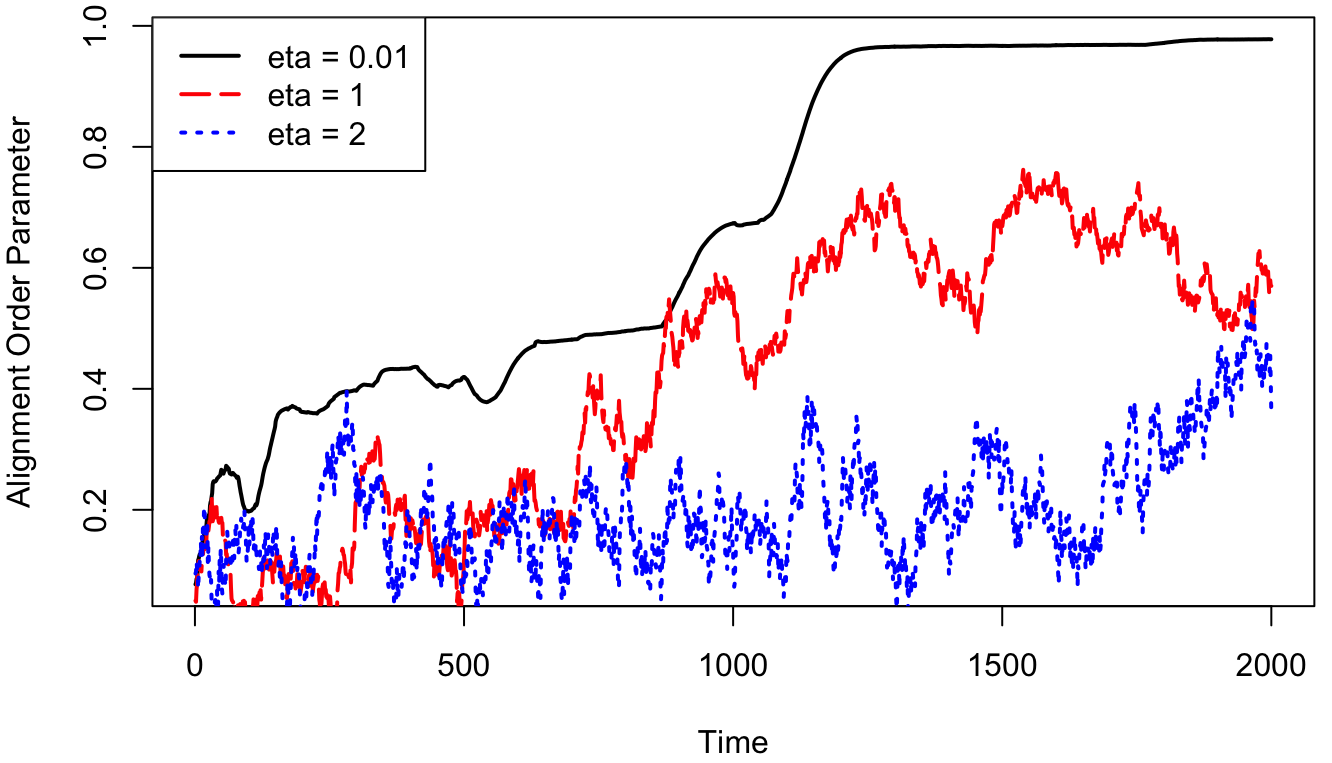
Figure 8 displays the alignment order parameters for three simulations with different noise parameters , , , and their changes over time. At time zero, all three values of the order parameter are quite low due to the random initialization of headings. All three simulations exhibit some alignment over time, with the smaller noise parameters reflecting a higher level of synchrony, consistent with Vicsek’s description above.
5.2.4. Crockers
Crocker plots, -smoothed crocker plots, and crocker stacks (collectively referred to as crockers) are three inputs that we will test in our machine learning experiments. We compute persistent homology using the R software package “TDA” [28], subsampling to every 10 time steps to speed up computations. At each subsampled time, we compute the persistent homology of Vietoris–Rips filtered simplicial complexes, with vertex set given by the scaled location and heading of each agent. We then compute the crockers from these persistent homology intervals over all times.
We make the following choices in the computations of our crockers.
- •
We only compute persistent homology in dimensions zero and one.
- •
We compute the Vietoris–Rips filtration up to scale parameter . These computations are discretized to consider 50 equally-spaced values of between and , inclusive.
- •
We consider 18 different smoothing values: from to inclusive, with steps of size in between.


Figure 9 is an example of an crocker plot for a simulation with noise parameter . We display only the contours of Betti numbers , interpreting larger contours as noise. In Figure 9, notice the large region with two connected components, namely , over the time range from approximately to 2000. This can be interpreted as two connected components for a wide range of both scale parameter and simulation time . By looking only at the -smoothed crocker plot, there is a priori no guarantee that these are the same components as scale varies. However, since the crocker stack contains enough information to recover the persistent homology barcodes, one can confirm these are the same connected components as varies by considering the later smoothings in the crocker stack. To verify these are the same connected components also as time varies, one would instead want to look at the vineyard representation.
Figure 10 illustrates a stack of -smoothed and crocker plots for the same simulation, with the values , , and shown. In , the Betti curves translate down as increases; by contrast, in , the Betti curves morph shapes as increases.
We will cluster different simulations based on their crocker representations, including crocker plots, single -smoothed crocker plots, and a crocker stack, and we compare the clustering accuracies in Section 5.3.
5.2.5. Experiments
We create four different experiments of increasing levels of clustering difficulty by considering different collections of noise values that we will try to predict from simulated data.
- •
Experiment 1. Five values: , , , , .
- •
Experiment 2. Three values: , , .
- •
Experiment 3. Six values: , , , , , .
- •
Experiment 4. Fifteen values: , , , , , , , , , , , , , , .
Note that the more similar is, the more difficult it will be to cluster the data correctly. As a thought experiment, consider two simulations with and , respectively. Both simulations will very quickly produce an aligned group, and once the groups are aligned, they are nearly indistinguishable. The most distinguishing data is during the transient times, but due to the quick equilibration of the system, there is relatively little transient data.
In all four experiments, we use time step equal to 10 for the crockers; additionally, we compute the crocker plot for time step equal to 40 in Experiment 2 to see how subsampling time affects accuracy. When computing the order parameter, we instead use time step equal to 1 (in order to get the “best” result the order parameter can provide); in Experiment 2, we also compute the order parameter with time step equal to 10 and 40 for comparison purposes.
5.2.6. Distance matrices
In each experiment, we vectorize the order parameter time series and crocker representations for each simulation, calculate the pairwise Euclidean distance between those vectors, and summarize the distances in a pairwise distance matrix. To vectorize the crocker representations, we take the crocker matrix (or -smoothed crocker matrix) and concatenate the rows, and for the crocker stack, we further concatenate each level of . Images of distance matrices for the order parameter and crocker plot (where the and vectorized crocker plots have been concatenated) are shown in Figures 11–14 for each of the four experiments, respectively. The distance matrices for crocker stacks are visually similar to those for crocker plots and thus will not be shown here. In each of the four pairs of comparisons, the crocker distance matrix is more structured than the order parameter distance matrix. This is consistent with the higher clustering accuracy based on crocker plots compared to order parameters, which we discuss in Section 5.3. That is, distances between simulations arising from the same (or similar) noise parameter(s) typically have a smaller distance than those from different noise parameters, resulting in a block structure in the crocker distance matrix that is not as apparent in the order parameter distance matrix.


5.2.7. Clustering method: -medoids
We use the -medoids algorithm to cluster the simulations from each experiment [35, 50]. This algorithm minimizes the sum of pairwise dissimilarities between data points by searching for objects from the data set, called medoids, and then partitioning the remaining observations to their closest medoid, resulting in clusters. The medoid is the most centrally located object of each cluster and is, in fact, an observation from the data set. Specifically, a medoid will correspond to a particular simulation in our clustering experiments which we can trace back to the underlying noise parameter of the simulation. The -medoids algorithm is often more robust than the ubiquitous -means algorithm, which minimizes the sum of squared Euclidean distance and thus, is more sensitive to outliers [4]. Another benefit of -medoids is that it can take as input a distance matrix, rather than a set of feature vectors, which will be important in Section 5.3.3 where we compute a distance on stacked sets of persistence diagrams which do not have vector representations.
We use the Partitioning Around Medoids (PAM) algorithm in the R package “cluster” [39] to perform the -medoids algorithm, setting to be equal to the number of distinct noise parameter values in each experiment. For instance, in Experiment 1, and in Experiment 4. We compute the classification accuracy as the percentage of simulations found to be in a cluster whose medoid comes from the same noise parameter value. Simulations partitioned into a cluster whose medoid does not come from the same noise parameter are misclassified.
5.2.8. PCA vs. non-PCA
The vectorized version of the alignment order parameter has 2001 time values ( to 2000), and accordingly the time series are of dimension 2001. On the other hand, a crocker plot, which has been downsampled by a factor of 10, has 201 time values and 50 values, resulting in a 10050-dimensional vectorized crocker for and , and resulting in a 20100-dimensional vectorized crocker for the concatenation . It might not be “fair” to directly compare the clustering results based on the different kinds of vectors of vastly differing dimensions. To address this problem, we reduce the dimension of each vector to three using Principal Component Analysis (PCA) [33]. This is reasonable as the first three principal components of each kind of feature vector capture about 90% of the variance. After reducing both the order parameter and crocker vectors for each simulation to 3-dimensional vectors, we create distance matrices based on the PCA-reduced vectors for each experiment, and then compare the PCA clustering accuracy with non-PCA clustering accuracy.
5.3. Key findings
5.3.1. Results summary
Table 1 shows a summary of the accuracies from clustering using -medoids on each of the four experiments with different input feature vectors (order parameters, crocker plots, and crocker stacks) using both the full representations (non-PCA) and dimensionality reduced versions (PCA, italicized). When we refer to the crocker stacks in the table, we are considering the stack of the 18 -smoothed crocker plots discussed in Section 5.2.4, where we vectorize the crocker for each and then concatenate. In Section 5.3.2, we consider the clustering accuracy of single -smoothed crocker plots in comparison with this stacked version. The crocker representations consider the homology dimensions and as well as the concatenation of the two.
| Exp. 1 | Exp. 2 | Exp. 3 | Exp. 4 | |||||
| Order Parameters | 0.63 | 0.51 | 0.61 | 0.59 | 0.35 | 0.35 | 0.21 | 0.17 |
| Crocker Plots, | 1.00 | 1.00 | 0.67 | 0.67 | 0.44 | 0.43 | 0.42 | 0.43 |
| Crocker Plots, | 1.00 | 1.00 | 0.67 | 0.77 | 0.45 | 0.43 | 0.39 | 0.43 |
| Crocker Plots, | 0.98 | 0.99 | 0.71 | 0.67 | 0.36 | 0.35 | 0.37 | 0.33 |
| Crocker Stacks, | 1.00 | 0.98 | 0.67 | 0.67 | 0.47 | 0.38 | 0.41 | 0.35 |
| Crocker Stacks, | 1.00 | 1.00 | 0.67 | 0.67 | 0.49 | 0.46 | 0.41 | 0.41 |
| Crocker Stacks, | 0.96 | 0.98 | 0.63 | 0.67 | 0.34 | 0.37 | 0.32 | 0.35 |
Crocker plot and stack clustering accuracies are higher than order parameter accuracies across all experiments. We perform paired sample t-tests to compare the means of experiment accuracies between order parameter and crocker plot () feature vectors and between order parameter and crocker stack () feature vectors. The 1-tail p-value for the t-test between order parameters and crocker plots is , and the p-value for the t-test between order parameters and crocker stacks is , which are both significant at the significance criterion level. In other words, the means of the four experiments’ accuracies for both crocker plots and stacks are significantly higher than for order parameters. As expected, Experiment 1 accuracy is the highest compared to other experiments for both order parameters and crocker plots. This is because the noise parameters are approximately evenly spaced in Experiment 1. Experiment 4 accuracy is the lowest, since Experiment 4 has both close and very different parameters, which confuses classification. Generally speaking, PCA (shown in italics in Table 1) and non-PCA accuracies are comparable across all four experiments. It is striking to us that even though we have reduced the dimension of the data down to 3 via PCA, we observe little degradation in cluster accuracy. The accuracies for crocker stacks are comparable with those for crocker plots.
Since distance matrices generally contain more information than either and , they often generate higher clustering accuracies than either or . We observe two exceptions for non-dimensionality reduced crocker plots: accuracy for Experiment 2 is slightly higher than and accuracy; accuracy for Experiment 3 is slightly higher than and accuracy. For non-dimensionality reduced croker stacks, accuracy is slightly higher than in Experiment 3.
Among order parameters, crocker plots, and crocker stacks, the stacks encode the most information, since they contain -smoothed crocker plots over several different values. In , the contour lines of -smoothed crocker plots continuously shift down as increases. This is because, in a Vietoris-Rips complex, all vertices are born at scale . Thus, the contour lines separating different ranks in the crocker plot translate as increases, but are otherwise unchanged. In contrast, in , the contour lines of -smoothed crocker plots do not continuously shift down but morph in shape. See the links for videos of and crocker stacks from a simulation corresponding to noise parameter of the Viscek model.
To further detail how the clustering accuracies in Table 1 arise, we consider Experiment 3 as a case study. Misclassifications can occur for two reasons. First, as alluded to previously, it will be very difficult to accurately cluster simulations that have different values of that are all in the small-noise regime, leading to strong alignment of the system. When the system aligns strongly and quickly, information contained in the transient state is lost. Second, even when the system is not in the strong-alignment regime, misclassifications may occur simply when values of are sufficiently close together. These difficulties are exemplified in Table 2, which shows the confusion matrix of the crocker plots of Experiment 3 clustered using -medoids, which contains simulations with = 0.01, 0.02, 0.19, 0.2, 1.99. The rows represent the actual simulations corresponding to each noise parameter while the columns represent the parameter of the cluster medoid to which a simulation is assigned. Even though clusters were formed, the six medoids correspond to simulations from only three distinct noise parameters , , . That is, there were two medoids from each of these three noise parameter classes selected by the algorithm, and we group clusters with the same noise parameter together. All simulations corresponding to noise parameters , , are misclassified as there are no medoids selected from these parameter classes.
| -medoids Clusters | |||
| = 0.02 | = 0.20 | = 2.00 | |
| = 0.01 | 69 | 31 | 0 |
| = 0.02 | 64 | 36 | 0 |
| = 0.19 | 4 | 96 | 99 |
| = 0.2 | 1 | 99 | 0 |
| = 1.99 | 0 | 0 | 100 |
| = 2.00 | 0 | 0 | 100 |
Notice that 69 of 100 simulations from class = 0.01 are partitioned into a cluster with a medoid coming from class , and 64 of 100 simulations from class = 0.02 are partitioned into the same cluster. This pattern is consistent for simulations with values of the same order of magnitude: simulations from classes and 0.2 are largely partitioned into a cluster with a medoid coming from class , and simulations from classes and 2 are all partitioned into a cluster with a medoid coming from class . In addition, simulations from the first four classes ( = 0.01, 0.02, 0.19, 0.2) are partitioned into either of the clusters with medoids from or 0.2. Recall that values of that are in the alignment regime will produce data that is essentially identical apart from a very brief transient phase and hence, are difficult to distinguish.
We now consider the effect of subsampling time on classification accuracy. The order parameter clustering accuracy for Experiment 2 with time step 1 is 0.61, and this is the same as subsampling the data by time steps of 10 and 40. In addition, the crocker plot and crocker stack accuracy for Experiment 2 with time steps 10 and 40 are the same. This shows that the effect of these subsamplings of time on clustering accuracy is negligible in this particular experiment.
5.3.2. smoothed crocker plots: stack vs. single ’s
We compare the clustering accuracy of the stacked -smoothed crocker plots (with 18 values combined) and those with a single value in Table 3. The crocker stack performs comparably to the individual -smoothed crocker plots.
As increases, accuracy decreases. This makes sense because as increases, more smoothing of distinct topological features occurs, which may ignore some information necessary for parameter identification.
| Exp. 1 | Exp. 2 | Exp. 3 | Exp. 4 | |
|---|---|---|---|---|
| stack | 1.00 | 0.67 | 0.47 | 0.41 |
| = 0.00 | 1.00 | 0.67 | 0.44 | 0.42 |
| = 0.01 | 1.00 | 0.67 | 0.46 | 0.40 |
| = 0.03 | 1.00 | 0.67 | 0.49 | 0.40 |
| = 0.05 | 1.00 | 0.58 | 0.44 | 0.38 |
| = 0.08 | 0.99 | 0.67 | 0.39 | 0.36 |
| = 0.11 | 0.97 | 0.67 | 0.33 | 0.35 |
| = 0.13 | 0.92 | 0.73 | 0.41 | 0.28 |
| = 0.17 | 0.73 | 0.66 | 0.40 | 0.21 |
5.3.3. Distances on stacked sets of persistence diagrams
We now want to compare the clustering accuracy of the crocker plot representations to the stacked set of persistence diagrams representation. Recall as introduced in Section 3.1, the latter can be thought of as time-varying persistence diagrams, since they contain the births and deaths of topological features over the scale parameter and time . Suppose two time-varying metric spaces X and Y have persistence diagrams and for all . One way to compute distance between these stacked sets of persistence diagrams is to compute the bottleneck distance between each pair of persistence diagrams and at each time and then take the supremum of the bottleneck distances over all time values. This supremum bottleneck distance (which we henceforth refer to as the bottleneck distance between stacked sets of persistence diagrams) is defined as follows:
As this computation is extremely expensive, we only compute this bottleneck distance for Experiment 2, which entails 300 simulations. The -medoids clustering accuracies based on this bottleneck distance matrix, along with corresponding accuracies of the Euclidean distances of the order parameters, crocker plots, and crocker stacks, are shown in Table 4.
| Order Parameters | (0.61) | (0.61) |
|---|---|---|
| Crocker Plots | 0.67 | 0.71 |
| Crocker Stacks | 0.67 | 0.63 |
| Stacked Persistence Diagrams | 0.67 | 0.49 |
As a stacked set of persistence diagrams is not a vector representation of the topological features, it cannot be directly fed into a machine learning algorithm as a feature vector. However, the -medoids clustering algorithm can take as input a distance matrix rather than a set of feature vectors. The pairwise bottleneck distance between stacked sets of persistence diagrams corresponding to simulations serves as our input for -medoids. As shown in Table 4, clustering with the bottleneck distance yields higher accuracy in but lower in as compared to order parameters. While we compute the order parameter at every time step in order to provide the “best” possible results, we downsample in time with a step size of 10 for the bottleneck computation due to computational complexity. The clustering accuracy for stacked persistence diagrams is either the same as or lower than crocker plots.
We now contrast the computational complexities for computing bottleneck distances of stacked persistence diagrams and Euclidean distances of crocker plots or stacks. Both processes start with the persistent homology data from our simulations over time. While we can directly compute the bottleneck distance between simulations from the interval data at a fixed time and then find the supremum over all times, in the crocker representations, we first need to transform the interval data to crocker plots or stacks, vectorize the crocker representation, and then compute the pairwise Euclidean distance between simulations. Even though there is a transformational step to convert the interval data into the crocker representations, the computational time for bottleneck distance matrices is roughly four orders of magnitude larger than for Euclidean distance matrices, including the transformation to crockers. Since clustering with stacked persistence diagrams does not yield higher clustering accuracy for this experiment and is far more time-intensive than the crocker representations, we posit that crockers may serve as a better means for parameter identification. Further, as crockers are vector representations, they are more amenable to a host of machine learning tools.
This concludes our experimental analysis of parameter identification of the Vicsek model using order parameters, crocker plots, crocker stacks, and stacked sets of persistence diagrams.
6. Distances between metric spaces and persistence modules
We now survey a variety of notions of distances between metric spaces and persistence modules, which will be useful for describing the continuity properties of crocker stacks in Section 7.
6.1. The Hausdorff distance
In order to introduce the stability of persistent homology, we will need some notion of distance on metric spaces. The Hausdorff distance [46] measures the distance between metric spaces and that are “aligned”. More precisely, we mean that and are subsets of a larger metric space that contains both and as submetric spaces. For and , let denote the -offset of in .
Definition 6.1.
If and are two subsets of a metric space , then the Hausdorff distance between and is , which is equivalent to
An illustration of the Hausdorff distance is shown in Figure 15.

The Hausdorff distance is an extended pseudo-metric on the subsets of ; two sets have Hausdorff distance zero if and only if they have the same closure, and the Hausdorff distance between unbounded sets can be infinite. When restricted to the set of all non-empty compact subsets of , the Hausdorff distance is in fact a metric. We often write , instead of , in order to simplify notation when space is clear.
6.2. Gromov–Hausdorff distance
The Gromov–Hausdorff distance [9] allows us to define a notion of distance between two metric spaces that are not aligned in any sense.
Definition 6.2.
The Gromov–Hausdorff distance between two metric spaces and is
where the infimum is taken over all possible metric spaces and isometric embeddings and .
The Gromov–Hausdorff distance is an extended pseudo-metric on metric spaces (non-isometric spaces, such as the rationals and the reals, can have Gromov–Hausdorff distance zero). The Gromov–Hausdorff distance is a metric when restricted to the quotient space of compact metric spaces under the equivalence relation of isometry.
6.3. The stability of persistent homology
By the stability of persistent homology [18, Theorem 5.2], if and are compact metric spaces, then the bottleneck distance satisfies
An analogous bound is true if Vietoris–Rips complexes are replaced with Čech complexes.
In many applications, spaces and are usually already embedded in the same space, in which one can use the bound in order to get a lower bound on the Hausdorff distance between these particular embeddings. The stability theorem states that if two metric spaces are close, then the bottleneck distance between their persistence diagrams (using the Vietoris–Rips or Čech complex to construct the filtration) will also be close. Stability is a useful property as it allows for small perturbations of the inputs, and as such, stability of persistence modules has led to their effectiveness in data analysis. One of our motivations for defining crocker stacks is their analogous continuity properties.
6.4. The interleaving distance
A closely related notion to the bottleneck distance between persistence diagrams associated to persistence modules (Section 2.4) is that of -interleaving [49].
Definition 6.3.
For two persistence modules and , a -interleaving (for ) is given by two families of linear maps () and () such that the following diagrams commute for all :
Note that a -interleaving between two persistence modules is nothing more than an isomorphism between them. The interleaving distance between persistence modules and is defined as
Roughly speaking, one should think of the interleaving distance between two persistence modules as a measure of how far they are from being isomorphic.
In this paper, we do not directly use the interleaving distance on persistence modules. However, by the isometry theorem of Lesnick [38], the interleaving distance is equal to the bottleneck distance, namely . As such, whenever we invoke the bottleneck distance, we could alternatively invoke the interleaving distance on persistence modules. The morphisms induced on the persistence modules by interleaving will allow us to prove Lemma 6.4, which is helpful for describing the continuity of crocker stacks.
6.5. The rank invariant
Let be a persistence module. We recall that the collection of all natural numbers for all choices of is called the rank invariant. The rank invariant is equivalent to the peristence barcode, in the sense that it is possible to obtain either one from the other [15, Theorem 12]. An interesting historical comment is that persistent homology of a finite set of points was first defined as the collection of ranks of all maps of the form , as opposed to as a persistence module, barcode, or diagram. See for example the definition on page 151 of [27], where their is , and where their is .
Given a persistence module , we can encode the rank invariant for as a function , where . The function is a function on a 2D domain, where the two dimensions are scale and persistence parameter .
We describe a connection between one time-slice of a crocker stack and the rank invariant. Let be a time-varying persistence module, and consider a fixed time . The 2D representation , for a fixed time , is a cross-sectional slice of the 3D crocker stack. Therefore, a crocker stack encodes the rank invariant, and therefore the persistence barcode, of the persistence module at each time . Persistence lanscapes can be interpreted as a sequence of rank functions, and therefore persistence landscapes [7] are also closely related to these cross-sectional slices (fixing time) in a crocker stack.
6.6. Relationship of rank invariant and bottleneck distance
We now describe a relationship between the rank invariant and the bottleneck distance. We consider two persistence modules and which decompose into a finite number of intervals, equipped with rank invariants and .
Lemma 6.4.
If , then for all and we have
- •
, and
- •
.
Proof.
By the equivalence between the bottleneck and interleaving distances of persistence modules [38, 49], since , there exist morphisms and for all , along with the following commutative diagrams.
Indeed, note that the trapezoids above can be obtained by gluing together a parallelogram and a triangle from Definition 6.3. Define to be the map from to . By the first commutative diagram, = . Since the rank of a composition of linear transformations is at most the minimum rank of the transformations, we have
Thus, , and so .
A similar argument for the second diagram shows . ∎
We remark that the infimum such that and for all and is the erosion distance [51, 26, 24, 53] between the two persistence modules and . Lemma 6.4 shows that if two persistence modules are close in the bottleneck distance (), then their rank invariants are also close in a sense encapsulated by the erosion distance (). Could a bound in the reverse direction also be true?
Question 1.
Is the bottleneck distance equal to the erosion distance between and , i.e., the infimum over all such that
- •
, and
- •
for all and ?
The answer is no, as shown by an example proposed by Amit Patel and Brittany Terese Fasy.
Example 1.

Consider persistence diagrams
as shown in Figure 16. The bottleneck distance between the two persistence diagrams is 1.5. There are two natural bijections between the two persistence modules, not including matching points with the diagonal (which in this example leads to higher costs). In bijection (i), we match in with in and in with in . The distance between matched points is 1.5. In bijection (ii), we match in with in and in with in . The distance between matched points is 2. The bottleneck distance is the infimum distance between matched points over all bijections, which is 1.5.
The erosion distance is the infimum such that for all and , we have , and . For this example, , for the following reasons: The maximum interval over which has rank two is , whereas the maximum interval over which has rank two is , and these regions differ by at most in their endpoints. Similarly, the maximum interval over which has rank at least one is over , whereas the maximal intervals over which has rank at least one is over either or : enlarging by on either endpoint covers either of these intervals in , and enlarging by on either endpoint covers . This is an intuitive explanation why for all and , we have
In this example, the bottleneck distance () is larger than the erosion distance (), answering Question 1 in the negative.
According to personal correspondence with Patel and Fasy, there is an algorithm for computing the erosion distance, where is the number of points in the diagram, which is much faster than computing the bottleneck distance. While Question 1 reveals that the two distances are not equivalent, the erosion distance could serve as a bound on the bottleneck distance. The rank invariants are also Möbius inversions of persistence diagrams [52, 40].
7. Continuity of crocker stacks
If two time-varying metric spaces are close to one another, then it turns out that the resulting crocker stacks are also (in some sense) close to one another. This is referred to as the continuity of crocker stacks. We explain why crocker plots are not continuous, before describing the sense in which crocker stacks are continuous.
7.1. Discontinuity of crocker plots
We first point out that crocker plots are not continuous.
Example 2.
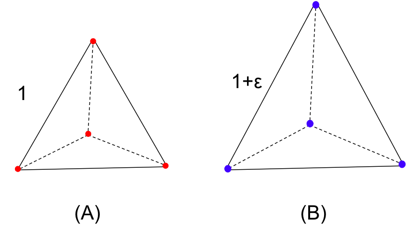
Suppose we have two dynamic metric spaces, each with 4 points in the metric space, as shown in Figure 17. In the first dynamic metric space , the distance between any two points is 1 for all times . In the second dynamic metric space , the distance between any two points is for all times . The two dynamic metric spaces are -close in the Gromov–Hausdorff distance. However, at scale parameter , the first dynamic metric space at any time has 0-dimensional Betti number . Yet at any time in the second dynamic metric space, at this same scale value. Thus, these Betti numbers differ by at scale . By increasing points to (say) points or beyond, we can make the values of these Betti numbers as far apart as we want. Under most notions of matrix distance, this would make the distance between the crocker plot matrices as far apart as we want, all while keeping the metric spaces within in the Gromov–Hausdorff distance. This example does not rely on time; it is really an example showing why Betti curves are not stable (in the traditional sense of distance between curves).
7.2. Distances between time-varying metric spaces
In order to describe the continuity properties of crocker stacks, we begin with some preliminaries on distances between time-varying metric spaces and time-varying persistence modules.
Definition 7.1.
Let and be continuous time-varying metric spaces over , and fix . The -Gromov–Hausdorff distance between and is
When we have .
To see that this is well-defined, note that since and are continuous, the function defined by is a continuous function over a closed interval, and hence is integrable.
We remark that this is only a pseudo-metric, not an actual metric. Indeed, as pointed out in Figure 1 of [37], two distinct time-varying metric spaces that are not qualitatively similar can have Gromov–Hausdorff distance zero from each other at each time . The distances between multiparameter rank functions introduced in [37] are also stable with respect to more refined notions of distance between time-varying metric spaces. In this paper, we restrict attention to the weaker Definition 7.1 and show that crocker stacks, which are amenable for machine learning tasks, are furthermore a continuous topological invariant.
7.3. Distances between time-varying persistence modules
We define an bottleneck distance between corresponding time-varying persistence modules.
Definition 7.2.
Let and be continuous time-varying persistence modules over , and fix . The -bottleneck distance between and is . When we have .
Since and are continuous, the function defined by is a continuous function over a closed interval, and hence is integrable.
Recall that our time-varying metric spaces are defined to have the property that is compact for all .
Lemma 7.3.
If and are continuous time-varying metric spaces over , then for all we have .
An analogous bound is true if Vietoris–Rips complexes are replaced with Čech complexes.
Proof.
Let . For any , we have by the stability of persistent homology. Integrating over all gives
The same proof works for by replacing integrals with supremums. Indeed,
∎
7.4. Continuity of crocker stacks
The continuity of a stacked set of persistence diagrams in the section above implies a continuity result for crocker stacks. Recall from Definition 4.1 that if is a time-varying persistence module, then
Suppose two time-varying metric spaces and have the property that and are within Hausdorff distance at all times . The interleaving distance between the persistence modules and is at most at all times . Hence, for all , , and , we have that and , where by an abuse of notation we let and denote and . This can be thought of as a notion of continuity, since it says the crocker stack for is in some sense “close” to the crocker stack for . In this subsection, we provide proofs for these observations.
Lemma 7.4.
If and are time-varying persistence modules, and if , then for all , , and we have
- •
, and
- •
.
Proof.
By hypothesis, we have for all . From Lemma 6.4 we have and for all . The conclusion follows since, by definition, we have and for all , , and . ∎
Note that a version of the above lemma for instead of would not give inequalities for each but instead a single pair of inequalities that are integrated (in an sense) over all .
The following theorem says that if the time-varying metric spaces and are nearby, then their crocker stacks are also close. Recall that our time-varying metric spaces are defined to be compact at each point in time.
Theorem 7.5 (Continuity theorem for crocker stacks).
If and are time-varying metric spaces, and if , then the crocker stacks for and are close in the sense that for all , , and , we have
- •
, and
- •
.
An analogous result is true if crocker stacks are defined using Čech complexes in place of Vietoris–Rips complexes.
Though crocker stacks are continous in the above sense, we want to acknowledge that they are not continuous when they are interpreted as vectors equipped with the Euclidean norm, which was the norm we used on crocker stacks in Section 5. More work remains to be done on effectively and stably vectorizing time-varying topological summaries for use in machine learning applications.
8. Conclusion
In this paper, we have provided an overview of topological tools for summarizing time-varying metric spaces, developed a new tool called the crocker stack, investigated the discriminative power of topological descriptors on a parameter recovery task, and discussed notions of continuity for these representations.
The crocker plot introduced in [56] is a topological summary of time-varying data. It has been shown in [56, 57, 6] to be useful in exploratory data analysis, statistical tests, and machine learning tasks. However, the crocker plot is not stable in any sense. We proposed the crocker stack as an alternative, which—like the crocker plot—can be discretized and treated as a vector in Euclidean space, making it useful in machine learning. Yet, the crocker stack also satisfies a continuity property, albeit with respect to a non-Euclidean metric.
A crocker stack is a 3D topological representation of a time-varying metric space that, like the crocker plot, displays all times in a single frame indexed by smoothing parameter . This may be better for visualization purposes than, say, the vineyard representation. Vineyards or stacked sets of persistence diagrams would have to be further vectorized for use in machine learning, perhaps by using say, persistence images [2]. The stable multiparameter rank function and distance measures in [37] are more discriminatory for time-varying metric spaces than the (pseudo-)distances we consider, but it is not obvious how to vectorize them for use in machine learning.
Through computational experiments, we show that crocker plots and stacks are more effective than the alignment order parameter, a traditional method derived from physics, at parameter identification in an ubiquitous model of biological aggregations. However, computing crocker plots and stacks are more time-intensive than computing order parameters. At each time step, a single number—the normalized average velocity—is computed in the order parameter, while persistent homology is computed in order to produce crocker plots and stacks. In our experiments, computing persistent homology is roughly two orders of magnitude more expensive than computing order parameters. The discriminative capability of the crocker representations may provide benefits that outweigh this computational complexity, however.
We end with a collection of questions and possible directions for researchers to explore.
- (1)
How do different choices of metrics affect the discriminatory power of crocker stacks in Section 5? For every and , there exists a metric on crocker stacks: to compare two fixed persistence diagrams, we can choose any and use an Wasserstein distance. To compare two time-varying persistence diagrams, we then could weight these distances over all times by choosing any averaging.
- (2)
What is the discriminatory power of a time-varying erosion distance say, for example, in the experiments in Section 5?
- (3)
- (4)
What are other notions of time-varying topological invariants that are both stable and also vectorizable in a way that is useful in machine learning?
Acknowledgments
We are grateful to Matraiyee Deka, Brittany Terese Fasy, Tom Halverson, Michael Lesnik, Dmitriy Morozov, and Amit Patel for helpful conversations.
References
- [1] H. Adams and G. Carlsson, Evasion paths in mobile sensor networks, International Journal of Robotics Research, 34 (2015), 90–104.
- [2] H. Adams, T. Emerson, M. Kirby, R. Neville, C. Peterson, P. Shipman, S. Chepushtanova, E. Hanson, F. Motta and L. Ziegelmeier, Persistence images: A stable vector representation of persistent homology, Journal of Machine Learning Research, 18 (2017), 1–35, URL http://jmlr.org/papers/v18/16-337.html.
- [3] H. Adams, D. Ghosh, C. Mask, W. Ott and K. Williams, Efficient evader detection in mobile sensor networks, arXiv preprint arXiv:2101.09813.
- [4] P. Arora, D. Deepali and S. Varshney, Analysis of K-means and K-medoids algorithm for big data, Procedia Computer Science, 78 (2016), 507–512.
- [5] A. Banman and L. Ziegelmeier, Mind the gap: A study in global development through persistent homology, in Research in Computational Topology, Springer, 2018, 125–144.
- [6] D. Bhaskar, A. Manhart, J. Milzman, J. T. Nardini, K. M. Storey, C. M. Topaz and L. Ziegelmeier, Analyzing collective motion with machine learning and topology, Chaos: An Interdisciplinary Journal of Nonlinear Science, 29 (2019), 123125.
- [7] P. Bubenik, Statistical topological data analysis using persistence landscapes, Journal of Machine Learning Research, 16 (2015), 77–102.
- [8] P. Bubenik, Statistical topological data analysis using persistence landscapes, The Journal of Machine Learning Research, 16 (2015), 77–102.
- [9] D. Burago, Y. Burago and S. Ivanov, A course in metric geometry, vol. 33, American Mathematical Society, Providence, 2001.
- [10] G. Carlsson, Topology and data, Bulletin of the American Mathematical Society, 46 (2009), 255–308.
- [11] G. Carlsson and V. de Silva, Zigzag persistence, Foundations of Computational Mathematics, 10 (2010), 367–405.
- [12] G. Carlsson, V. de Silva, S. Kališnik and D. Morozov, Parametrized homology via zigzag persistence, Algebraic & Geometric Topology, 19 (2019), 657–700.
- [13] G. Carlsson, V. De Silva and D. Morozov, Zigzag persistent homology and real-valued functions, in Proceedings of the twenty-fifth annual symposium on Computational geometry, ACM, 2009, 247–256.
- [14] G. Carlsson, G. Singh and A. Zomorodian, Computing multidimensional persistence, in International Symposium on Algorithms and Computation, Springer, 2009, 730–739.
- [15] G. Carlsson and A. Zomorodian, The theory of multidimensional persistence, Discrete & Computational Geometry, 42 (2009), 71–93.
- [16] A. Cerri, B. D. Fabio, M. Ferri, P. Frosini and C. Landi, Betti numbers in multidimensional persistent homology are stable functions, Mathematical Methods in the Applied Sciences, 36 (2013), 1543–1557.
- [17] W. Chacholski, M. Scolamiero and F. Vaccarino, Combinatorial presentation of multidimensional persistent homology, Journal of Pure and Applied Algebra, 221 (2017), 1055–1075.
- [18] F. Chazal, V. de Silva and S. Oudot, Persistence stability for geometric complexes, Geometriae Dedicata, 174 (2014), 193–214.
- [19] D. Cohen-Steiner, H. Edelsbrunner and D. Morozov, Vines and vineyards by updating persistence in linear time, in Proceedings of the twenty-second annual symposium on Computational geometry, ACM, 2006, 119–126.
- [20] P. Corcoran and C. B. Jones, Modelling topological features of swarm behaviour in space and time with persistence landscapes, IEEE Access, 5 (2017), 18534–18544.
- [21] D. B. Damiano and M. R. McGuirl, A topological analysis of targeted in-111 uptake in spect images of murine tumors, Journal of mathematical biology, 76 (2018), 1559–1587.
- [22] V. de Silva and R. Ghrist, Coordinate-free coverage in sensor networks with controlled boundaries via homology, The International Journal of Robotics Research, 25 (2006), 1205–1222.
- [23] V. de Silva and R. Ghrist, Coverage in sensor networks via persistent homology, Algebraic & Geometric Topology, 7 (2007), 339–358.
- [24] T. K. Dey and C. Xin, Computing bottleneck distance for 2-d interval decomposable modules, CoRR, abs/1803.02869.
- [25] M. R. D’Orsogna, Y. L. Chuang, A. L. Bertozzi and L. S. Chayes, Self-propelled particles with soft-core interactions: Patterns, stability, and collapse, Phys. Rev. Lett., 96 (2006), 104302, URL https://link.aps.org/doi/10.1103/PhysRevLett.96.104302.
- [26] H. Edelsbrunner, D. Morozov and A. Patel, The stability of the apparent contour of an orientable 2-manifold, Topological Methods in Data Analysis and Visualization. Mathematics and Visualization., 27–41.
- [27] H. Edelsbrunner and J. L. Harer, Computational Topology: An Introduction, American Mathematical Society, Providence, 2010.
- [28] B. T. Fasy, J. Kim, F. Lecci, C. Maria, D. L. Millman and V. Rouvreau, Tda: Statistical tools for topological data analysis, https://cran.r-project.org/web/packages/TDA/index.html.
- [29] M. Feng and M. A. Porter, Persistent homology of geospatial data: A case study with voting, arXiv preprint arXiv:1902.05911.
- [30] M. Feng and M. A. Porter, Spatial applications of topological data analysis: Cities, snowflakes, random structures, and spiders spinning under the influence, Phys. Rev. Research, 2 (2020), 033426.
- [31] R. Ghrist, Barcodes: The persistent topology of data, Bulletin of the American Mathematical Society, 45 (2008), 61–75.
- [32] C. Giusti, L. Papadopoulos, E. T. Owens, K. E. Daniels and D. S. Bassett, Topological and geometric measurements of force-chain structure, Physical Review E, 94 (2016), 032909.
- [33] I. Jolliffe, Principal Component Analysis, Springer Verlag, 1986.
- [34] T. Kaczynski, K. Mischaikow and M. Mrozek, Computational homology, vol. 157, Springer Science & Business Media, 2006.
- [35] L. Kaufman and P. Rousseeuw, Clustering by means of medoids, North-Holland, 1987.
- [36] W. Kim and F. Mémoli, Stable signatures for dynamic metric spaces via zigzag persistent homology, arXiv preprint arXiv:1712.04064.
- [37] W. Kim and F. Mémoli, Spatiotemporal persistent homology for dynamic metric spaces, Discrete & Computational Geometry, 1–45.
- [38] M. Lesnick, The theory of the interleaving distance on multidimensional persistence modules, Foundations of Computational Mathematics, 15 (2015), 613–650.
- [39] M. Maechler, Finding groups in data: Cluster analysis extended rousseeuw et al, https://cran.r-project.org/web/packages/cluster/cluster.pdf.
- [40] A. McCleary and A. Patel, Bottleneck stability for generalized persistence diagrams, Proceedings of the American Mathematical Society, 148 (2020), 3149–3161.
- [41] A. McCleary and A. Patel, Edit distance and persistence diagrams over lattices, arXiv preprint arXiv:2010.07337.
- [42] E. Miller, Data structures for real multiparameter persistence modules, arXiv preprint arXiv:1709.08155.
- [43] N. Milosavljević, D. Morozov and P. Skraba, Zigzag persistent homology in matrix multiplication time, in Proceedings of the twenty-seventh annual symposium on Computational geometry, 2011, 216–225.
- [44] D. Morozov, Personal communication.
- [45] D. Morozov, Dionysus, URL http://www.mrzv.org/software/dionysus/.
- [46] J. R. Munkres, Topology, Prentice-Hall Englewood Cliffs, NJ, 1975.
- [47] C. Nilsen, J. Paige, O. Warner, B. Mayhew, R. Sutley, M. Lam, A. J. Bernoff and C. M. Topaz, Social Aggregation in Pea Aphids: Experiment and Random Walk Modeling, PLoS ONE, 8 (2013), e83343, URL http://dx.doi.org/10.1371/journal.pone.0083343.
- [48] N. Otter, M. A. Porter, U. Tillmann, P. Grindrod and H. A. Harrington, A roadmap for the computation of persistent homology, EPJ Data Science, 6 (2017), 17.
- [49] S. Y. Oudot, Persistence theory: From quiver representations to data analysis, vol. 209, American Mathematical Society Providence, RI, 2015.
- [50] H.-S. Park and C.-H. Jun, A simple and fast algorithm for -medoids clustering, Expert Systems with Applications, 36 (2009), 3336–3341.
- [51] A. Patel, Generalized persistence diagrams, J Appl. and Comput. Topology, 1 (2018), 397–419.
- [52] A. Patel, Generalized persistence diagrams, Journal of Applied and Computational Topology, 1 (2018), 397–419.
- [53] V. Puuska, Erosion distance for generalized persistence modules, Homology, Homotopy, and Applications, 22 (2020), 233–254.
- [54] M. Scolamiero, W. Chachólski, A. Lundman, R. Ramanujam and S. Öberg, Multidimensional persistence and noise, Foundations of Computational Mathematics, 17 (2017), 1367–1406.
- [55] B. J. Stolz, H. A. Harrington and M. A. Porter, Persistent homology of time-dependent functional networks constructed from coupled time series, Chaos: An Interdisciplinary Journal of Nonlinear Science, 27 (2017), 047410.
- [56] C. M. Topaz, L. Ziegelmeier and T. Halverson, Topological data analysis of biological aggregation models, PloS one, 10 (2015), e0126383.
- [57] M. Ulmer, L. Ziegelmeier and C. M. Topaz, A topological approach to selecting models of biological experiments, PloS one, 14 (2019), e0213679.
- [58] T. Vicsek, A. Czirók, E. Ben-Jacob, I. Cohen and O. Shochet, Novel type of phase transition in a system of self-driven particles, Phys. Rev. Lett., 75 (1995), 1226–1229, URL https://link.aps.org/doi/10.1103/PhysRevLett.75.1226.
- [59] X. Zhu, Persistent homology: An introduction and a new text representation for natural language processing, in Twenty-Third International Joint Conference on Artificial Intelligence, 2013.
- [60] A. Zomorodian and G. Carlsson, Computing persistent homology, Discrete Comput. Geom., 33 (2005), 249–274.