Deep Autoencoder based Energy Method for the Bending, Vibration, and Buckling Analysis of Kirchhoff PlatesJournal: European Journal of Mechanics / A Solids
Abstract
In this paper, we present a deep autoencoder based energy method (DAEM) for the bending, vibration and buckling analysis of Kirchhoff plates. The DAEM exploits the higher order continuity of the DAEM and integrates a deep autoencoder and the minimum total potential principle in one framework yielding an unsupervised feature learning method. The DAEM is a specific type of feedforward deep neural network (DNN) and can also serve as function approximator. With robust feature extraction capacity, the DAEM can more efficiently identify patterns behind the whole energy system, such as the field variables, natural frequency and critical buckling load factor studied in this paper. The objective function is to minimize the total potential energy. The DAEM performs unsupervised learning based on random generated points inside the physical domain so that the total potential energy is minimized at all points. For vibration and buckling analysis, the loss function is constructed based on Rayleigh’s principle and the fundamental frequency and the critical buckling load is extracted. A scaled hyperbolic tangent activation function for the underlying mechanical model is presented which meets the continuity requirement and alleviates the gradient vanishing/explosive problems under bending analysis. The DAEM can be easily implemented and we employed the Pytorch library and the LBFGS optimizer. A comprehensive study of the DAEM configuration is performed for several numerical examples with various geometries, load conditions, and boundary conditions.
Keywords:
Deep learning, Autoencoder, Activation function, Energy method, Kirchhoff plate, Vibration, Buckling.1 Introduction
Thin plate models are commonly used in engineering and mechanics [1] due to their computational efficiency. Their mechanical analysis are of major importance in engineering practice. Due to the limitations of analytical methods, a variety of numerical methods have been developed including the finite element method [2, 3], boundary element method [4, 5], meshfree method [6, 7], isogeometric analysis (IGA) formulations [8], numerical manifold method [9, 10, 11] and recently deep learning based methods [12, 13, 14].
Deep learning was proposed in 2006 [15, 16]. It is an unsupervised feature learning method with neural network architectures including multiple hidden layers [17]. Equipped with this hierarchical structure, it can extract information from complicated raw input data with multiple levels of abstraction through a layer-by-layer process [18]. Various variants such as multilayer perceptron (MLP), convolutional neural networks (CNN) and recurrent/recursive neural networks (RNN) [19] have been developed and applied to e.g. image processing [20, 21], object detection [22, 23], speech recognition [24, 25], biology [26, 27] and even finance [28, 29].
Artificial neural networks (ANN) can be traced back to the 1940’s [30] but they became especially popular in the past few decades due to the vast development in computer science and computational science such as backpropagation technique and advances in deep neural networks. Due to the simplicity and feasibility of ANNs to deal with nonlinear and mult-dimensional problems, they were applied in inference and identification by data scientists [31]. They were also adopted to solve partial differential equations (PDEs) [32, 33, 34] but shallow ANNs are unable to learn the complex nonlinear patterns effectively. With improved theories incorporating unsupervised pre-training, stacks of auto-encoder variants, and deep belief nets, deep learning has become also an interesting alternative to classical methods such as FEM.
According to the universal approximation theorem [35, 36], any continuous function can be approximated by a feedforward neural network with one single hidden layer. However, the number of neurons of the hidden layer tends to increase exponentially with increasing complexity and non-linearity of a model. Recent studies show that DNNs render better approximations for nonlinear functions [37]. Some researchers employed deep learning for the solution of PDEs. E et al. developed a deep learning-based numerical method for high-dimensional parabolic PDEs and back-forward stochastic differential equations [38, 39]. Raissi et al. [40] introduced physics-informed neural networks for supervised learning of nonlinear partial differential equations. Beck et al. [41] employed deep learning to solve nonlinear stochastic differential equations and Kolmogorov equations. Sirignano and Spiliopoulos [42] provided a theoretical proof for deep neural networks as PDE approximators, and concluded that it converged as the number of hidden layers tend to infinity. Anitescu et al. [12], Guo et al. [13], and Nguyen-Thanh et al. [14] applied deep neural networks for finding the solutions for second and forth order boundary value problems.
The learning ability of deep neural networks has been enhanced with different architectures, such as deep belief network (DBN) or deep autoencoder (DAE) [43, 44]. DAE is widely used in dimensionality reduction and feature learning. It has also been proven to be an effective way to learn and describe latent codes that reflect meaningful variations in data with an encoding and decoding layer [45]. DAE seems therefore ideally suited for learning and describing the underlying physical patterns from the governing partial differential equation or associated potential energy. In this paper, we therefore propose a deep autoencoder based energy learning method for Kirchhoff plate analysis. In this context, we exploit the higher order continuity of the DAE approximation.
The paper is organised as follows: First, we describe the Kirhhoff plate model. Then we introduce the basic elements of the deep autoencoder theory, and present a tailored activation function for this mechanical model. Subsequently, the deep autoencoder based energy method is presented. Finally, we demonstrate the efficiency and accuracy of the DAEM for various benchmark problems.
2 Kirchhoff plate model
Consider a Kirchhoff plate as shown in Figure 1. The displacement field can be expressed as:
| (2.1) | ||||
where the relation between lateral deflection of the middle surface and rotations about the ,-axis is given by
| (2.2) |
The transversal deflection of the mid-plane is regarded as field variable and the corresponding bending and twisting curvatures are generalized strains:
| (2.3) |
The geometric equations can be then obtained as:
| (2.4) |
with L being the differential operator defined as .
Accordingly, the bending and twisting moments shown in Figure 1 can be expressed as:
| (2.5) | ||||
Here, is the bending rigidity, and denote the Young’s modulus and Poisson ratio, and is the thickness of the thin plate. It can be rewritten in a Matrix form
| M=Dk | (2.6) |
with . The shear forces of the mid-surface is obtained in terms of the bending and twisting moments as
| (2.7) |
The boundary conditions can be categorized into three parts, namely,
| (2.8) |
At the clamped boundary, , are functions of the arc length along this boundary. At the simply supported edge boundary, , where is also a function of arc length along this boundary. At the free boundary conditions, , where is the load exerted along this boundary where corresponds to the normal and tangent directions along the boundaries.
The total potential energy consists of the strain energy U and the potential energy of the external forces W:
| (2.9) |
where
| (2.10) | ||||
and
| (2.11) |
with .
For vibration analysis assuming that the plate is undergoing harmonic vibrations, we can approximate the vibrating mid-surface of the plate by
| (2.12) |
The maximum kinetic energy can be obtained by choosing as
| (2.13) |
The maximum strain energy occurs when . Accounting for the , the lowest natural frequency of a vibrating plate can be obtained by setting:
| (2.14) |
where
The can be defined as
| (2.15) |
which will be used in the subsequent analysis.
Moreover, we will introduce the energy criterion to the classical eigenvalue buckling of Kirchhoff plates. Bifurcation of an initial configuration of equilibrium occurs [1] when the increment in the total potential energy of plate upon buckling equals zero:
| (2.16) |
The increment in the total potential energy of the plate upon buckling can be expressed as strain energy of the bending and twisting of a plate plus the work done by in-plane forces [1],
| (2.17) | |||
Here, can denotes the perturbed transverse deflection and in-plane forces can be chosen as with a reference value of the in-plane force. In practical application, is often set to be unity and thus becomes the desired buckling load factor and can be obtained from Equation 2.16:
| (2.18) |
which will also be used in the subsequent analysis. The minimum of the load parameter is the critical buckling load.
3 Basic theory of a deep autoencoder
In deep learning, engineers have further enhanced the learning ability of deep neural networks with different architectures, such as deep belief network (DBN) or deep autoencoder (DAE), to mention a few. Autoencoders play a fundamental role in unsupervised learning and are widely chosen deep architectures for dimensionality reduction and feature learning, which has been proven to be an effective way to learn and describe latent codes that reflect meaningful variations from raw input data.
3.1 Network architecture
Autoencoders are a specific type of feedforward neural networks including an encoder and a decoder. The basic structure is shown in Figure 2. The network reconstructs the input by mapping them from a high-dimensional space to a low-dimensional space enabling the hidden layer to learn a better representation of the input and the decoder layer then reconstructs the results to another space.
As shown in Figure 2, the fully connected feedforward neural network is composed of multiple layers: an input layer, one encoding layer, one "bottleneck" layer, one decoding layer and one output layer. Each layer consists of one or more nodes called neurons, indicated by small coloured circles in Figure 2. For the interconnected structure, every two neurons in neighbouring layers have a connection, which is represented by a connection weight. The weight between neuron in the hidden layer and neuron in hidden layer is denoted by . No connection exists among neurons in the same layer as well as in the non-neighbouring layers. Data flows through this neural network via connections between neurons, starting from the input layer, through the encoding layer over the hidden layer to the decoding layer and finally through the output layer. The autoencoder in Figure 2 consists of two parts: an encoder mapping:
| (3.1) |
and a decoding mapping
| (3.2) |
that produces a reconstruction. The autoencoder defines a mapping
| (3.3) |
Let be the nonlinear activation function on each layer. There are many choices for the activation function and we will propose an improved version of the -activiation function to analyse the mechanical response of Kirchhoff plates. Combined with weight and bias vector defined on each layer, the nonlinear mapping can be written as
| (3.4) |
Similarly, the decode maps can be written as
| (3.5) |
Default activation functions available in Pytorch such as the do not necessarily yield the best results for every model. We will show later in numerical experiments that it results sometimes in unstable results for the deep autoencoder based energy method (DAEM). Therefore, we suggest a modified activation function:
| (3.6) |
As shown later, this activation function yields better results due to the following reasons: 1.) A larger range of upper values are forced towards and a larger range of lower values are close to , with steeper gradients for the mid-range, which can be seen in Figure 3. Thus, the training is spread uniformly through the feedforward neural network. 2.) For Kirchhoff plate problems, Navier successfully solved those problems with trigonometric Fourier series. Considering that is periodically changing from to , it can be also adopted as activation function suitable for dynamic analysis. However, periodic activation functions might lead to a "rippling" cost function with bad local minima since a low and high input may produce the same output making the neural network very difficult to train. The hyperbolic functions, however, satisfy many identities analogous to the trigonometric identities and also map input between and . In this case, the scaled hyperbolic function is preferable, as it yields stable and accurate results and will not slow down the training process. This small change in the activation function has largely improved the Vanishing/Exploding gradient problems in the deep autoencoder neural networks for this model, as will be shown later. The modified new activation has been studied under different layers and different neurons for cases in which Vanishing/Exploding gradient problems are observed for the activation function.
Moreover, the number of neurons on each hidden layer and the number of hidden layers can be arbitrarily chosen and are invariably determined through a trial and error procedure or a pruning technique [46]. In the numerical example section, the detailed configuration of this deep autoencoder has been studied and offers an optimum selection of number of hidden layers while keeping the number of neurons on each layer small. An autoencoder thus defines a function depending on the input data x and parametrised by consisting of weights and biases in each layer. It provides an efficient way to approximate unknown field variables and identifies those physical codes behind the model.
3.2 Basic algorithm for backpropagation
Like other feedforeward neural networks, deep autoencoders can be trained with all techniques in deep learning such as minibatch gradient descent method with gradients computed by backpropagation. Backpropagation is an important and computationally efficient mathematical tool to compute gradients in deep learning [47]. Backpropagation has two main phases, propagation and weight update. The chain rule is recursively applied during the whole process.
For the deep autoencoder based energy method, first, the field variable is approximated by a deep autoencoder . The components of the linear strain tensor are derivatives of the field variable and can be approximate by a set of deep autoencoder sharing the same hyperparameters. In order to find the hyperparameters of the deep autoencoder including weights and biases, a loss function is constructed [48]. The backpropagation algorithm for the deep autoencoder can be summarised as:
- •
Input: Input dataset , prepare activation for input layer;
- •
Feedforward: For each layer , compute , and ;
- •
Output error: Compute the error
- •
Backpropagation error: For each , compute ;
- •
Output: The gradient of the loss function is given by and .
Here, denotes the Hadamard product.
4 Deep autoencoder based energy method
Different from our previous work on deep collocation [13], the energy method starts from the principle of minimum energy and finds the solution by minimizing the total potential energy of this system. The energy method is a weak formulation, which has several advantages over the deep collocation method which is based on the strong form. Firstly, the continuity requirements for the approximating function is reduced in the energy based method requiring less gradient computations compared to the deep collocation method. And secondly, natural boundary condition are automatically satisfied in the energy method, which is especially helpful for fourth order problems.
4.1 Energy method for bending analysis
Let us consider Kirchhoff plate bending problems in the context of the DAEM. Recalling Equation 2.9 is the total potential energy, the entire problem can be boiled down to minimizing the total potential energy enforcing essential boundary conditions. The transversal deflection is approximated with the aforementioned deep autoencoder denoted by . A loss function can thus be constructed to find the approximate solution by minimizing of total potential energy with essential boundary conditions approximated by . Substituting into Equation 2.9, Equation 2.10, and Equation 2.12, results in
| (4.1) |
where
| (4.2) | |||
and
| (4.3) | |||
with , which yields an energy driven deep neural network . Moreover, , , and can be obtained by substituting into Equation 2.3. The boundary conditions from Section 2 can also be learnt by the neural network approximation : On , we have
| (4.4) |
On ,
| (4.6) |
where can be obtained from Equation 2.5 and can be obtained from Equation 2.7 by combing . Note that refer to the normal and tangent directions along the boundaries. The induced energy driven neural network shares the same parameters as .
Finally, we construction the loss function for the proposed DAEM, which minimizes the total potential energy subjected to essential boundary conditions:
| (4.7) |
with
| (4.8) | ||||
where , ; , are the neural network parameters and , is a solution to transversal deflection.
Note that the proposed DAEM requires a method to evaluate the integrals and also the corresponding quadrature points are deployed as input datasets. We could adopt ’traditional’ multivariate numerical quadrature methods such as Gaussian quadrature. A background mesh could therefore be constructed. However, minimizing the total potential energy at those fixed points might results in underfitting. This issue can be avoided by random sampling and therefore, the Monte Carlo integration method [49] is employed in DAEM for the integral calculation. For the two dimensional Monte-Carlo integration method, let us consider the integral in Equation 4.3, which can be evaluated by
| (4.9) |
denoting the dataset generated by the ramdom sampling in the physical domain and is the area of the middle surface and is the number of random distributed points inside the physical domain.
4.2 Energy method for vibration and buckling analysis
The loss function for the vibration and buckling analysis has to be modified. The key objective is to obtain the fundamental natural frequency and critical buckling, respectively. Recalling Equation 2.15, the Rayleigh quotient is defined and derived from Rayleigh’s principle and the lowest natural frequency can be retrieved from the minimization of Equation 2.15 accounting for essential boundary conditions. Also the mode shape function is approximated by the deep autoencoder . Accordingly, the loss function can be defined as:
| (4.10) |
with
| (4.11) | ||||
where , ; , are the neural network parameters. The Monte-Carlo quadrature rule is adopted for calculating the Rayleigh quotient. However, some modification to the loss function is needed to ensure is a nontrivial solution. Therefore, we normalize the mode shape function and ensure the inner product of the mode shape function is unity. This leads to the modified loss function
| (4.12) |
where is a penalty factor. A factor between 1 to 100 already yields good numerical results. The loss function for the buckling analysis can be written as
| (4.13) |
where is the load factor. From Equation 2.18, we obtain
| (4.14) |
where is the approximation of the transversal deflection by the deep autoencoder, i.e. . Now, we can find the set of parameters such that the approximated deflection minimizes the loss , i.e.
| (4.15) |
These hyperparameters are obtained by backpropogation as mentioned before. The L-BFGS [50] optimizer with backpropogation is adopted to tune those hyperparameters of the deep autoencoder with few restrictions. Thus, the solution to thin plate bending, vibration and buckling problems by deep autoencoder based energy method can be reduced to an optimization problem. The general procedure of the proposed DAEM can be summarized as follows:
-
[rightmargin=label=()]
- 1.
calculate activation function on hidden layers in Equation 3.4.
- 2.
calculate the reconstructed output from in Equation 3.5.
- 3.
- 4.
back-propogate error gradient and update weights and bias
5 Numerical Experiments
In this section, we demonstrate the performance of DAEM for several numerical examples for plate bending, vibration and buckling analysis. The simulations are done on a 64-bit macOS Mojave server with Intel(R) Core(TM) i7-8850H CPU, 32GB memory. We found that a deep neural structure with less width is preferred over a shallow structures. Hence, we mainly show results for increasing number of hidden layers rather than for increasing number of neurons. The accuracy of the numerical results by using the relative error of maximum deflection and deflection over the whole plate. The relative error is defined as:
| (5.1) |
Here, refers to the .
5.1 Bending analysis
We study three benchmark problems including a plate with hole and a plate on the elastic foundation, which can be compared to an analytical solution.
5.2 Square plate under a sinusoidally distributed load
Let us consider a simply-supported square plate under a sinusoidal distribution transverse loading. The sinusoidal distributed load is expressed by
| (5.2) |
where , indicate the length of the plate. The analytical solution for this problem is given by [51]:
| (5.3) |
We first study the accuracy and efficiency of the proposed activation function. In general, the test is performed with a deep feedforward neural network with 10 neurons per hidden layer. The relative error of the maximum deflection at the central plate and the deflection over the whole plate vs the increasing of hidden layers are shown in Figure 4. The modified hyperbolic tangent activation function is less dependent on the number of hidden layers than the original hyperbolic tangent activation function.
The computational cost of those two schemes is shown in Figure 5 and is comparable. The relative error of the deflection is shown in Table 1. While the gradient explodes for some problems – indicated by NaN (not a real number) – for the original activation function, the modified activation function always yields stable results. The encoding configuration refers here to the hidden layers and neuron numbers specified for the encoder. For the decoder a symmetric configuration is adopted.
| Relative Error of Deflection | ||
|---|---|---|
| Encoder Configuration | ||
| Encoding layer, [30] | 0,0063740 | 0,0060618 |
| Encoding layer, [40] | NaN | 0,0058869 |
| Encoding layer, [50] | 0,0130702 | 0,0090355 |
| Encoding layer, [60] | 0,0077438 | 0,0104713 |
| Encoding layers, [30,10] | 0,0083107 | 0,0070922 |
| Encoding layers, [40,10] | 0,0082238 | 0,0066074 |
| Encoding layers, [50,10] | 0,0061002 | 0,0082771 |
| Encoding layers, [60,10] | 0,0075465 | 0,0058044 |
| Encoding layers, [30,20] | 0,0075115 | 0,0078926 |
| Encoding layers, [40,20] | 0,0087727 | 0,0086784 |
| Encoding layers, [50,20] | NaN | 0,0055310 |
| Encoding layers, [60,20] | NaN | 0,0084229 |
| Encoding layers, [30,20,10] | 0,0083553 | 0,0069302 |
| Encoding layers, [50,30,10] | 0,0121318 | 0,0077830 |
| Encoding layers, [60,30,10] | 0,0102968 | 0,0053692 |
| Encoding layers, [40,30,20] | 0,0075632 | 0,0075470 |
| Encoding layers, [50,30,20] | 0,0067328 | 0,0065867 |
| Encoding layers, [60,30,20] | NaN | 0,0060054 |
Next, we study the recommended deep autoencoder configuration by comparing various encoders with varying layers and neurons per layer. As shown in Figure 6, an increasing number of encoding layers results – as expected – in increased computational cost.

The relative errors obtained by different encoder schemes are shown in Figure 7. The results converge to the analytical solution with increasing number of layers. However, more neurons do not necessarily improve the accuracy, especially for encoder . Moreover, the results are already quite accurate with only one encoding layer. In summary, these numerical experiments suggest the change of the DAEM layer configuration rather than increasing the width of the deep neural network.

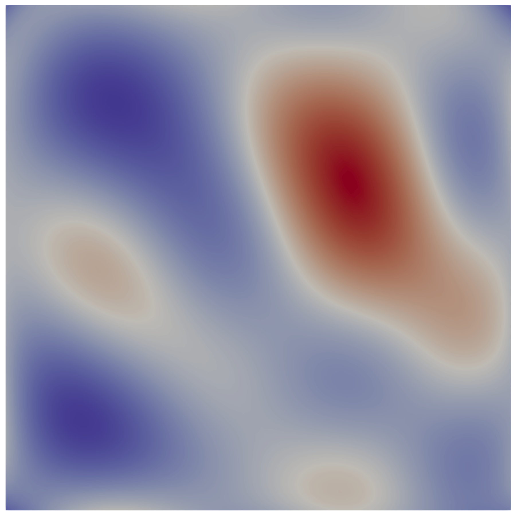
Next, we test the influence of quadrature points on the accuracy of the solution by calculating the relative error of the maximum deflection and deflection. A series of randomly distributed quadrature points ranging from are used to calculate the integrals. The numerical results are shown in Figure 8. Associated contour plots are illustrated in Figure 9.

5.2.1 Annular Plate under uniformly distributed pressure
Next, we study an annular plate, which is simply-supported on the outer circle and free on the inner circle. The analytical solution of this problem is [51]:
| (5.4) |
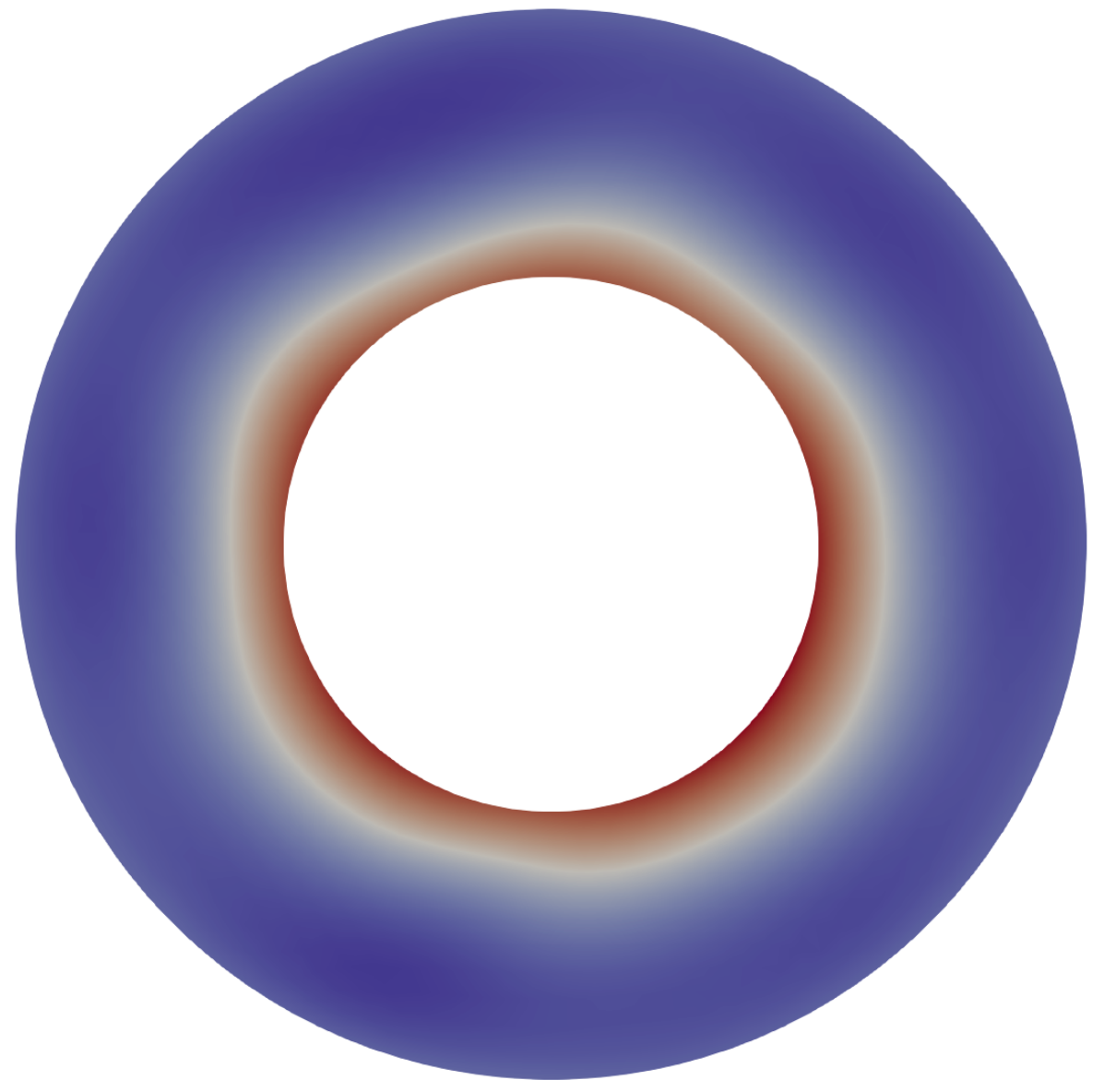
where , , , , , being the outer and inner radius of the annular plate, respectively. We also show results for a referennce point and study different activation functions. We again observe the exploding gradient problem for DAEM with the activation function, which can be alleviated by the , see Figure 10. Contour plots of the deflection and absolute deflection are depicted in Figure 11 showing that the predicted deflection agrees well with the analytical solution.

5.2.2 Square plate on Winkler foundation
Finally, we study a simply-supported plate on Winkler foundation assuming the foundation’s reaction is expressed by , k being the foundation modulus. For a plate on a continuous Winkler foundation, the potential energy needs to be added to the total potential energy, Equation 4.1:
| (5.5) |
The analytical deflection is given by [51]:
| (5.6) |
Different configurations of the deep autoencoder are tested. The relative errors in the deflection and maximum deflection are shown in Figure 12 and 13, respectively. Increasing the layers leads to more accurate results with increasing encoding layers. For some cases, increasing the width of the neural network does not improve the results, so that a deep neural network is preferable. The computational cost is depicted in Figure 14. As expected, more encoding layers increases the computational cost. However, note that this includes also the training cost. Once the network has been trained, the solution will be obtained much faster.


5.3 Vibration analysis
We now apply DAEM to extract the fundamental frequency in a transversal vibration analysis. The results are compared with reference solutions from [52, 53, 54, 55]. Let us consider a square plate with a square cutout as shown in Figure 15, is the ratio of the inner to outer square size. Various boundary conditions are studied. The non-dimensional fundamental frequency parameter with different cutout ratio is studied. A deep autoencoder with encoding layers is adopted as this architecture provided accurate results for the bending analysis while being computationally efficient.
The nondimensional fundamental frequency is depcited in Table 2. The predicted results agree well with reference results of the HBM method [52], Modified Ritz method [53], FEM [53], and Discrete Ritz method [55].
| Non-dimensional fundamental frequency parameter | |||||
| Cutout ratio | DAEM | HBM method | Modified Ritz method | FEM | Discrete Ritz method |
| 0 | 19,7382 | 19,7390 | 19,7400 | 19,7520 | 19,7390 |
| 0,1 | 19,3508 | 19,4440 | 19,1830 | 19,3570 | 19,4130 |
| 0,2 | 19,0284 | 19,1280 | 18,7620 | 19,1200 | 19,0380 |
| 0,3 | 19,3834 | 19,4450 | 19,1830 | 19,3570 | 19,3910 |
| 0,4 | 20,8201 | 20,7530 | 20,7850 | 20,7320 | 20,7240 |
| 0,5 | 23,4641 | 23,4530 | 23,6640 | 23,2350 | 23,4410 |
| 0,6 | 28,2706 | 28,3750 | 28,8440 | 28,2410 | 28,5260 |
| 0,7 | 38,1596 | 37,5720 | 38,1580 | 35,5790 | 37,8920 |
| 0,8 | 58,0804 | 57,4120 | 58,0620 | 57,4520 | 57,8380 |
| 0,9 | 120,9580 | 120,0200 | 121,2300 | 120,3900 | 120,9900 |
The fundamental mode shapes for different cutout ratios are shown in Table 3 and agree well with results in [52].
| Cutout ratio | Fundamental mode shape | Cutout ratio | Fundamental mode shape |
|---|---|---|---|
| 0 |
![[Uncaptioned image]](2010.05698v1/VibSSh00.png)
|
0,5 |
![[Uncaptioned image]](2010.05698v1/VibSSh05.png)
|
| 0,1 |
![[Uncaptioned image]](2010.05698v1/VibSSh01.png)
|
0,6 |
![[Uncaptioned image]](2010.05698v1/VibSSh06.png)
|
| 0,2 |
![[Uncaptioned image]](2010.05698v1/VibSSh02.png)
|
0,7 |
![[Uncaptioned image]](2010.05698v1/VibSSh07.png)
|
| 0,3 |
![[Uncaptioned image]](2010.05698v1/VibSSh03.png)
|
0,8 |
![[Uncaptioned image]](2010.05698v1/VibSSh08.png)
|
| 0,4 |
![[Uncaptioned image]](2010.05698v1/VibSSh04.png)
|
0,9 |
![[Uncaptioned image]](2010.05698v1/VibSSh09.png)
|
Next, we perform a vibration analysis of the square plate for two other boundary conditions, i.e. 1: all outer edges are clamped and 2. two opposite outer edges are clamped, while the other two outer edges are simply-supported. The cutout ratio of this square plate is selected to be . The results are summarized in Table 4 and agree well with results from [52].
| Boundary Conditions | Fundamental mode shape | |
|---|---|---|
| CCCC | 49,3091 |
![[Uncaptioned image]](2010.05698v1/VibCCh04.png)
|
| CSCS | 35,4996 |
![[Uncaptioned image]](2010.05698v1/VibCSh04.png)
|
5.4 Buckling analysis
Finally, we study a skew plate with different skew angles and aspect ratio subjected to uniaxial inplane compressive loading, see Figure 16. We consider simply-supported and clamped boundary conditions. The effects of the skew angle, aspect ratio on the critical buckling load factor are computed and compared with the reference solution presented in [56].
| Non-dimensional critical buckling load parameter | ||||||
| Aspect ratio | Skew angle | DAEM | Rayleigh-Ritz method | FEM | CQUAD4 | CQUAD8 |
| 0,5 | 0∘ | 6,2575 | 6,2500 | 6,2510 | 6,2010 | 6,2180 |
| 0,5 | 15∘ | 7,0172 | 7,0000 | 6,9800 | 6,8550 | 6,9080 |
| 0,5 | 30∘ | 9,9614 | 10,0200 | 9,9400 | 9,8950 | 10,0000 |
| 0,5 | 45∘ | 19,4074 | 19,3000 | 9,4200 | 18,9510 | 19,2520 |
| 1 | 0∘ | 4,0007 | 4,0000 | 4,0000 | 3,9190 | 4,0000 |
| 1 | 15∘ | 4,5073 | 4,4800 | 4,4000 | 4,3060 | 4,3550 |
| 1 | 30∘ | 5,8504 | 6,4100 | 5,9300 | 5,7610 | 5,8750 |
| 1 | 45∘ | 10,5208 | 12,3000 | 10,3600 | 9,5260 | 9,9540 |
| 1,5 | 0∘ | 4,3710 | 0,0000 | 0,0000 | 4,2560 | 4,2700 |
| 1,5 | 15∘ | 4,6558 | 4,7700 | 4,6800 | 4,6400 | 4,6480 |
| 1,5 | 30∘ | 5,9504 | 6,3700 | 5,8900 | 5,9550 | 5,8650 |
| 1,5 | 45∘ | 9,1843 | 10,9000 | 8,9500 | 9,0760 | 9,1390 |
| 2 | 0∘ | 3,9354 | 0,0000 | 0,0000 | 3,8850 | 3,9030 |
| 2 | 15∘ | 4,3499 | 4,3300 | 4,3400 | 4,2710 | 4,3130 |
| 2 | 30∘ | 5,5677 | 6,0300 | 5,5900 | 5,5960 | 5,6050 |
| 2 | 45∘ | 8,9418 | 10,3000 | 8,8000 | 8,8550 | 8,8710 |
The nonlinear encoding layer adopted in this study is , which is better suitable for varying geometries. The simply-supported skew plate is studied first and the associated results are shown in Table 5. The numerical results are compared with results of the Rayleigh-Ritz method, FEM, CQUAD4 and CQUAD8 [56]. As the skew angle increases, the critical buckling load parameter increases. For the clamped skew plate, we exemplary show results for the skew plate with aspect ratio . The numerical results can be found in Table 6. The predicted results agree well with the analytical solution.
| Non-dimensional critical buckling load parameter | |||||
| Skew angle | DAEM | Rayleigh-Ritz method | FEM | CQUAD4 | CQUAD8 |
| 0∘ | 10,0909 | 10,0000 | 10,0800 | 9,8540 | 10,0000 |
| 15∘ | 10,7821 | 10,9000 | 10,8400 | 10,6900 | 10,7750 |
| 30∘ | 13,7013 | 13,5800 | 13,6000 | 13,5030 | 13,5370 |
| 45∘ | 20,9890 | 20,4000 | 20,7600 | 20,0920 | 20,1050 |
| Aspect ratio | Buckling mode shape | Aspect ratio | Buckling mode shape |
|---|---|---|---|
| 0,5 |
![[Uncaptioned image]](2010.05698v1/BlkSSh05.png)
|
1 |
![[Uncaptioned image]](2010.05698v1/BlkSSh10.png)
|
| 1,5 |
![[Uncaptioned image]](2010.05698v1/BlkSSh15.png)
|
2 |
![[Uncaptioned image]](2010.05698v1/BlkSSh20.png)
|
Let us focus exemplary on the mode shape of the simply-supported plate with varying aspect ratios and a fixed skew angle of . The predicted mode shapes for each case are illustrated in Table 7. The buckling mode shapes for the clamped skew plate and a fixed aspect ratio of and varying skew angle are listed in Table 8. The predicted results agree well with the ones in [56]. Note that once the hyperparameters of this neural network are obtained, the network can be used to predict similar problems quickly and since the training is an unsupervised learning, no target value on the solution is needed.
| Skew angle | Buckling mode shape | Skew angle | Buckling mode shape |
|---|---|---|---|
| 0∘ |
![[Uncaptioned image]](2010.05698v1/BlkCC00.png)
|
15∘ |
![[Uncaptioned image]](2010.05698v1/BlkCC15.png)
|
| 30∘ |
![[Uncaptioned image]](2010.05698v1/BlkCC30.png)
|
45∘ |
![[Uncaptioned image]](2010.05698v1/BlkCC45.png)
|
6 Conclusions
In this paper, a deep autoencoder based energy method for bending, vibration and buckling analysis of Kirchhoff plate is proposed. For the proposed method, the deep autoencoder which is suitable for unsupervised feature extraction is combined with the minimum total potential energy principle to solve michanical analysis of Kirchhoff plate, and it has successfully discovered the underlying physical patterns. Moreover, a tailored activation is proposed for the deep autoencoder based energy method, which has been proven to be more stable and alleviated the gradient explosion problem without compromising computational efficiency. To calculate the total potential energy, the fitted Monte Carlo integration is adopted, and makes the whole method to be truly "meshfree" and very easily accessible. And once the deep autoencoder based energy method is trained, it can predict the physical features readily.
Further, the deep autoencoder based energy method has been applied to extracting funtamental frequency, critical buckling load and corresponding mode shapes based on Rayleigh’s principle. Different numerical examples covering various type of Kirchhoff plate models, including bending, vibration, buckling of plate with different geometries, cutout, boundary and load conditions and even on Winkler foundation have been investigated to validate the proposed method. The accuracy and efficiency of the proposed activation is studied and compared in numerical examples. Further, the favourable deep autoencoder configuration are studied to offer practical guidance for application. Though this is still a preliminary research, numerical experiments have demonstrated favourable features for this deep autoencoder method for prediction the physical patterns behind the Kirchhoff plate model. And the proposed autoencoder based energy method is more simple and efficient than the deep collocation method, so it can be further applied to more engineering fields.
However, those are just preliminary studies of this method. There are still several issues remain to be addressed, like a more suitable global optimization algorithm, and application to more complicated engineering problems, et al. Those are our future research projects, including the geometric and material nonlinear analysis in solid mechanics and computational fluid mechanics with deep autoencoder based energy method.
Reference
- [1] E. Ventsel, T. Krauthammer, Thin plates and shells: theory: analysis, and applications, CRC press, 2001.
- [2] K.-J. Bathe, Finite element procedures, Klaus-Jurgen Bathe, 2006.
- [3] T. J. Hughes, The finite element method: linear static and dynamic finite element analysis, Courier Corporation, 2012.
- [4] J. T. Katsikadelis, The boundary element method for engineers and scientists: theory and applications, Academic Press, 2016.
- [5] C. A. Brebbia, S. Walker, Boundary element techniques in engineering, Elsevier, 2016.
- [6]
V. P. Nguyen, T. Rabczuk, S. Bordas, M. Duflot,
Meshless
methods: A review and computer implementation aspects, Mathematics and
Computers in Simulation 79 (3) (2008) 763 – 813.
doi:https://doi.org/10.1016/j.matcom.2008.01.003.
URL http://www.sciencedirect.com/science/article/pii/S0378475408000062 - [7] T. Q. Bui, M. N. Nguyen, A moving kriging interpolation-based meshfree method for free vibration analysis of kirchhoff plates, Computers & structures 89 (3-4) (2011) 380–394.
- [8] V. P. Nguyen, C. Anitescu, S. P. Bordas, T. Rabczuk, Isogeometric analysis: an overview and computer implementation aspects, Mathematics and Computers in Simulation 117 (2015) 89–116.
- [9] H. Zheng, Z. Liu, X. Ge, Numerical manifold space of hermitian form and application to kirchhoff’s thin plate problems, International Journal for Numerical Methods in Engineering 95 (9) (2013) 721–739.
- [10] H. Guo, H. Zheng, The linear analysis of thin shell problems using the numerical manifold method, Thin-Walled Structures 124 (2018) 366–383.
- [11] H. Guo, H. Zheng, X. Zhuang, Numerical manifold method for vibration analysis of kirchhoff’s plates of arbitrary geometry, Applied Mathematical Modelling 66 (2019) 695–727.
- [12] C. Anitescu, E. Atroshchenko, N. Alajlan, T. Rabczuk, Artificial neural network methods for the solution of second order boundary value problems, Computers, Materials & Continua 59 (1) (2019) 345–359.
- [13] H. Guo, X. Zhuang, T. Rabczuk, A deep collocation method for the bending analysis of kirchhoff plate, CMC-COMPUTERS MATERIALS & CONTINUA 59 (2) (2019) 433–456.
- [14] V. M. Nguyen-Thanh, X. Zhuang, T. Rabczuk, A deep energy method for finite deformation hyperelasticity, European Journal of Mechanics-A/Solids (2019) 103874.
- [15] G. E. Hinton, S. Osindero, Y.-W. Teh, A fast learning algorithm for deep belief nets, Neural computation 18 (7) (2006) 1527–1554.
- [16] Y. Bengio, P. Lamblin, D. Popovici, H. Larochelle, Greedy layer-wise training of deep networks, in: Advances in neural information processing systems, 2007, pp. 153–160.
- [17] Y. LeCun, Y. Bengio, G. Hinton, Deep learning, nature 521 (7553) (2015) 436.
- [18] I. Goodfellow, Y. Bengio, A. Courville, Deep learning, MIT press, 2016.
- [19] J. Patterson, A. Gibson, Deep learning: A practitioner’s approach, " O’Reilly Media, Inc.", 2017.
- [20] L. Yang, A. MacEachren, P. Mitra, T. Onorati, Visually-enabled active deep learning for (geo) text and image classification: a review, ISPRS International Journal of Geo-Information 7 (2) (2018) 65.
- [21] D. S. Kermany, M. Goldbaum, W. Cai, C. C. Valentim, H. Liang, S. L. Baxter, A. McKeown, G. Yang, X. Wu, F. Yan, et al., Identifying medical diagnoses and treatable diseases by image-based deep learning, Cell 172 (5) (2018) 1122–1131.
- [22] W. Ouyang, X. Wang, X. Zeng, S. Qiu, P. Luo, Y. Tian, H. Li, S. Yang, Z. Wang, C.-C. Loy, et al., Deepid-net: Deformable deep convolutional neural networks for object detection, in: Proceedings of the IEEE conference on computer vision and pattern recognition, 2015, pp. 2403–2412.
- [23] Z.-Q. Zhao, P. Zheng, S. Xu, X. Wu, Object detection with deep learning: A review, IEEE transactions on neural networks and learning systems (2019).
- [24] D. Amodei, S. Ananthanarayanan, R. Anubhai, J. Bai, E. Battenberg, C. Case, J. Casper, B. Catanzaro, Q. Cheng, G. Chen, et al., Deep speech 2: End-to-end speech recognition in english and mandarin, in: International conference on machine learning, 2016, pp. 173–182.
- [25] A. B. Nassif, I. Shahin, I. Attili, M. Azzeh, K. Shaalan, Speech recognition using deep neural networks: a systematic review, IEEE Access (2019).
- [26] T. Yue, H. Wang, Deep learning for genomics: A concise overview, arXiv preprint arXiv:1802.00810 (2018).
- [27] T. Ching, D. S. Himmelstein, B. K. Beaulieu-Jones, A. A. Kalinin, B. T. Do, G. P. Way, E. Ferrero, P.-M. Agapow, M. Zietz, M. M. Hoffman, et al., Opportunities and obstacles for deep learning in biology and medicine, Journal of The Royal Society Interface 15 (141) (2018) 20170387.
- [28] J. Heaton, N. Polson, J. H. Witte, Deep learning for finance: deep portfolios, Applied Stochastic Models in Business and Industry 33 (1) (2017) 3–12.
- [29] T. Fischer, C. Krauss, Deep learning with long short-term memory networks for financial market predictions, European Journal of Operational Research 270 (2) (2018) 654–669.
- [30] W. S. McCulloch, W. Pitts, A logical calculus of the ideas immanent in nervous activity, The bulletin of mathematical biophysics 5 (4) (1943) 115–133.
- [31] F. M. Dias, A. Antunes, A. M. Mota, Artificial neural networks: a review of commercial hardware, Engineering Applications of Artificial Intelligence 17 (8) (2004) 945–952.
- [32] I. E. Lagaris, A. Likas, D. I. Fotiadis, Artificial neural networks for solving ordinary and partial differential equations, IEEE transactions on neural networks 9 (5) (1998) 987–1000.
- [33] I. E. Lagaris, A. C. Likas, D. G. Papageorgiou, Neural-network methods for boundary value problems with irregular boundaries, IEEE Transactions on Neural Networks 11 (5) (2000) 1041–1049.
- [34] K. S. McFall, J. R. Mahan, Artificial neural network method for solution of boundary value problems with exact satisfaction of arbitrary boundary conditions, IEEE Transactions on Neural Networks 20 (8) (2009) 1221–1233.
- [35]
K.-I. Funahashi,
On
the approximate realization of continuous mappings by neural networks,
Neural Networks 2 (3) (1989) 183 – 192.
doi:https://doi.org/10.1016/0893-6080(89)90003-8.
URL http://www.sciencedirect.com/science/article/pii/0893608089900038 - [36]
K. Hornik, M. Stinchcombe, H. White,
Multilayer
feedforward networks are universal approximators, Neural Networks 2 (5)
(1989) 359 – 366.
doi:https://doi.org/10.1016/0893-6080(89)90020-8.
URL http://www.sciencedirect.com/science/article/pii/0893608089900208 - [37] H. N. Mhaskar, T. Poggio, Deep vs. shallow networks: An approximation theory perspective, Analysis and Applications 14 (06) (2016) 829–848.
- [38] E. Weinan, J. Han, A. Jentzen, Deep learning-based numerical methods for high-dimensional parabolic partial differential equations and backward stochastic differential equations, Communications in Mathematics and Statistics 5 (4) (2017) 349–380.
- [39] J. Han, A. Jentzen, E. Weinan, Solving high-dimensional partial differential equations using deep learning, Proceedings of the National Academy of Sciences 115 (34) (2018) 8505–8510.
- [40]
M. Raissi, P. Perdikaris, G. Karniadakis,
Physics-informed
neural networks: A deep learning framework for solving forward and inverse
problems involving nonlinear partial differential equations, Journal of
Computational Physics 378 (2019) 686 – 707.
doi:https://doi.org/10.1016/j.jcp.2018.10.045.
URL http://www.sciencedirect.com/science/article/pii/S0021999118307125 - [41]
C. Beck, W. E, A. Jentzen,
Machine learning
approximation algorithms for high-dimensional fully nonlinear partial
differential equations and second-order backward stochastic differential
equations, Journal of Nonlinear Science (Jan 2019).
doi:10.1007/s00332-018-9525-3.
URL http://dx.doi.org/10.1007/s00332-018-9525-3 - [42] J. Sirignano, K. Spiliopoulos, Dgm: A deep learning algorithm for solving partial differential equations, Journal of Computational Physics 375 (2018) 1339–1364.
- [43] H. Shao, H. Jiang, H. Zhao, F. Wang, A novel deep autoencoder feature learning method for rotating machinery fault diagnosis, Mechanical Systems and Signal Processing 95 (2017) 187–204.
- [44] J. Yu, X. Zheng, S. Wang, A deep autoencoder feature learning method for process pattern recognition, Journal of Process Control 79 (2019) 1–15.
- [45] J. Snoek, R. P. Adams, H. Larochelle, Nonparametric guidance of autoencoder representations using label information, Journal of Machine Learning Research 13 (Sep) (2012) 2567–2588.
- [46] S. Anwar, K. Hwang, W. Sung, Structured pruning of deep convolutional neural networks, ACM Journal on Emerging Technologies in Computing Systems (JETC) 13 (3) (2017) 32.
- [47] M. A. Nielsen, Neural networks and deep learning, Vol. 25, Determination press San Francisco, CA, USA:, 2015.
- [48]
K. Janocha, W. M. Czarnecki,
On loss functions for
deep neural networks in classification, Schedae Informaticae 1/2016 (2017).
doi:10.4467/20838476si.16.004.6185.
URL http://dx.doi.org/10.4467/20838476SI.16.004.6185 - [49] R. E. Caflisch, Monte carlo and quasi-monte carlo methods, Acta Numerica 7 (1998) 1–49. doi:10.1017/S0962492900002804.
- [50] D. C. Liu, J. Nocedal, On the limited memory bfgs method for large scale optimization, Mathematical programming 45 (1-3) (1989) 503–528.
- [51] S. P. Timoshenko, S. Woinowsky-Krieger, Theory of plates and shells, McGraw-hill, 1959.
- [52]
Y. Zhang, C. Wang, D. Pedroso, H. Zhang,
Extension
of hencky bar-net model for vibration analysis of rectangular plates with
rectangular cutouts, Journal of Sound and Vibration 432 (2018) 65 – 87.
doi:https://doi.org/10.1016/j.jsv.2018.06.029.
URL http://www.sciencedirect.com/science/article/pii/S0022460X18303900 - [53]
K. Lam, K. Hung, S. Chow,
Vibration
analysis of plates with cutouts by the modified rayleigh-ritz method,
Applied Acoustics 28 (1) (1989) 49 – 60.
doi:https://doi.org/10.1016/0003-682X(89)90030-3.
URL http://www.sciencedirect.com/science/article/pii/0003682X89900303 - [54]
K. Liew, S. Kitipornchai, A. Leung, C. Lim,
Analysis
of the free vibration of rectangular plates with central cut-outs using the
discrete ritz method, International Journal of Mechanical Sciences 45 (5)
(2003) 941 – 959.
doi:https://doi.org/10.1016/S0020-7403(03)00109-7.
URL http://www.sciencedirect.com/science/article/pii/S0020740303001097 - [55]
I. Shufrin, M. Eisenberger,
Semi-analytical
modeling of cutouts in rectangular plates with variable thickness – free
vibration analysis, Applied Mathematical Modelling 40 (15) (2016) 6983 –
7000.
doi:https://doi.org/10.1016/j.apm.2016.02.020.
URL http://www.sciencedirect.com/science/article/pii/S0307904X16300944 - [56] C. Srinivasa, Y. Suresh, W. P. Kumar, Buckling studies on laminated composite skew plates, International Journal of Computer Applications 37 (1) (2012) 35–47.