Navier–Stokes transport coefficients for a model of a confined quasi-two-dimensional granular binary mixture
Abstract
The Navier–Stokes transport coefficients for a model of a confined quasi-two-dimensional granular binary mixture of inelastic hard spheres are determined from the Boltzmann kinetic equation. A normal or hydrodynamic solution to the Boltzmann equation is obtained via the Chapman–Enskog method for states near the local version of the homogeneous time-dependent state. The mass, momentum, and heat fluxes are determined to first order in the spatial gradients of the hydrodynamic fields, and the associated transport coefficients are identified. They are given in terms of the solutions of a set of coupled linear integral equations. In addition, in contrast to previous results obtained for low-density granular mixtures, there are also nonzero contributions to the first-order approximations to the partial temperatures and the cooling rate . Explicit forms for the diffusion transport coefficients, the shear viscosity coefficient, and the quantities and are obtained by assuming steady-state conditions and by considering the leading terms in a Sonine polynomial expansion. The above transport coefficients are given in terms of the coefficients of restitution, concentration, and the masses and diameters of the components of the mixture. The results apply in principle for arbitrary degree of inelasticity and are not limited to specific values of concentration, mass and/or size ratios. As a simple application of these results, the violation of the Onsager reciprocal relations for a confined granular mixture is quantified in terms of the parameter space of the problem.
I Introduction
Granular gases can be considered as a collection of discrete macroscopic particles (typically of the order of micrometers or larger). Normally, grains differ in size, mass or in their mechanical properties and, as a consequence, granular gases require a multicomponent description. Due to their macroscopic dimensions, in contrast to molecular or ordinary gases, all collisions between grains are inelastic and so the total kinetic energy of the particles decreases with time. Brilliantov and Pöschel 2004; Garzó 2019 Thus, on order to maintain the system in the so-called rapid flow regime, an external energy input is needed to inject energy into the system and compensate for the energy dissipated by collisions. When both mechanisms cancel each other the system achieves a steady nonequilibrium state. The injection of energy can be done for instance by vibrating walls Yang et al. 2002; Huan et al. 2004 or by bulk driving, as in air-fluidized beds. Abate and Durian 2006; Schröter, Goldman, and Swinney 2005 However, this way of providing energy develops in most cases strong spatial gradients and hence, the theoretical description of the system is quite complicated. To avoid the above problem, it is common in theoretical and computational studies to feed energy into the system by means of external driving forces or thermostats Puglisi et al. 1999; Cafiero, Luding, and Herrmann 2000; Prevost, Egolf, and Urbach 2002; Paganobarraga et al. 2002; Puglisi, Baldassarri, and Loreto 2002; Fiege, Aspelmeier, and Zippelius 2009; Kranz, Sperl, and Zippelius 2010; Vollmayr-Lee, Aspelmeier, and Zippelius 2011; Gradenigo et al. 2011; Puglisi et al. 2012. A remarkable observation is that the transport properties of granular systems not only depend on the mechanical properties of the grains, but also on the thermostating method (see, for example, the comparison between the Navier–Stokes shear viscosity obtained from the Chapman–Enskog expansion around the homogeneous cooling state Brey et al. 1998 and the non-Newtonian shear viscosity of the uniform shear flow state; Santos, Garzó, and Dufty 2004; Cordero, Risso, and Soto 2005 a detailed discussion on this issue can be found in Ref. Garzó 2019).
An alternative to the use of external forces has been proposed in the past few years. Olafsen and Urbach 1998; Prevost et al. 2004; Melby et al. 2005; Clerc et al. 2008; Pacheco-Vázquez, Caballero-Robledo, and Ruiz-Suárez 2009; Rivas et al. 2011; Castillo, Mújica, and Soto 2012; Mujica and Soto 2016 The idea is to employ a particular geometry where the granular gas is confined in a box whose -direction is slightly larger than one particle diameter, so particles are confined in the vertical direction. We refer to this geometry as a quasi-two-dimensional geometry. The box is vertically vibrated so that energy is injected into the vertical degrees of freedom of particles via the collisions of grains with the top and bottom plates. The energy gained by collisions with the walls is then transferred to the horizontal degrees of freedom when a collision between particles takes place. Under certain conditions, the system presents a liquid-solid like phase separation. Complementarily, it remains in a homogeneous fluidized state (when it is observed from above) for a wide range of parameters (see Ref. Mujica and Soto 2016 for a review of this geometry).
The full collisional dynamics in this geometry is highly complex, particularly due to the severe restrictions to the set of possible impact parameters imposed by the confinement. Maynar, García de Soria, and Brey 2019 To advance in the understanding of the quasi-two-dimensional geometry, a collisional model for the transfer of energy from the vertical to horizontal degrees of freedom was proposed years ago by Brito et al. Brito, Risso, and Soto 2013 As mentioned earlier, the vertical vibration accumulates energy into the -component of the velocity. In this model, particles move only in two-dimensions but, when a collision between particles occurs, part of the accumulated energy is released into the horizontal components of the velocity. In practice, an extra velocity is added to the relative motion of colliding spheres and hence, the magnitude of the normal component of the relative velocity is increased by a given factor in the collision. The magnitude of the factor can be related with the intensity of the vertical vibrations in the experiments. Maynar, García de Soria, and Brey 2019 For simplicity, is assumed to be constant; this choice has the advantage of adding only a single parameter to the conventional inelastic hard sphere (IHS) model. The parameter fixes the energy scale of the steady state. Moreover, it has been shown for constant that the system remains homogeneous for all values of the global density. Brito, Risso, and Soto 2013 A more realistic version of the above collisional model has been recently proposed Risso, Soto, and Guzmán 2018, where is assumed to be a function of the local density. Such model gives rise to a van der Waals loop and a phase separation, in agreement with experiments. Olafsen and Urbach 1998; Prevost et al. 2004; Melby et al. 2005; Clerc et al. 2008 However, the derivation of the hydrodynamic equations from this model is much more involved than that of the model where is constant since an additional hydrodynamic field is needed.
The collisional model with constant (referred here to as the -model) has been widely employed by several groups in the past few years to describe the properties of the quasi-two-dimensional geometry. In particular, Brey and coworkers have considered this model in the dilute regime (i) to analyze the homogeneous state, Brey et al. 2013; Brey et al. 2014 (ii) to derive the Navier–Stokes hydrodynamic equations with explicit forms for the corresponding transport coefficients, Brey et al. 2015 and (iii) to perform a linear stability analysis of the homogeneous time-dependent state. Brey et al. 2016 The shear viscosity of a dilute granular gas has been also independently determined Soto, Risso, and Brito 2014 and theoretical predictions compare quite well with computer simulations. The above previous works Brey et al. 2015; Soto, Risso, and Brito 2014 of the -model have been recently extended to moderate densities by considering the Enskog kinetic equation and explicit forms of the Navier–Stokes transport coefficients have been explicitly obtained in terms of the coefficient of restitution and the density. GBS18 In addition, very recently, the -model has been extended to binary mixtures where the lack of equipartition has been analyzed in the stationary state. Brito, Soto, and Garzó 2020 Besides this work, we are not aware of any previous study on granular hydrodynamics in the relevant case of multicomponent systems in the context of the -model.
The goal of this paper is to provide a description of hydrodynamics in binary granular mixtures at low density with a comparable accuracy to that for the monocomponent case, namely, valid over the broadest parameter range including strong inelasticity. Brey et al. 2015; Soto, Risso, and Brito 2014; GBS18 As a previous step, the reference homogeneous time-dependent state for a binary mixture has been discussed in detail recently. Brito, Soto, and Garzó 2020 The characterization of this reference state is crucial to provide the proper basis of transport due to spatial inhomogeneities.
As in previous works on granular mixtures, Garzó and Dufty 2002; Garzó, Montanero, and Dufty 2006; Serero et al. 2006; Garzó and Montanero 2007; Serero et al. 2009; Garzó, Murray, and Vega Reyes 2013 the Chapman–Enskog method Chapman and Cowling 1970 conveniently adapted to account for dissipative collisions is used to solve the coupled set of the Boltzmann equations for the two components. Garzó 2019 In the first order of spatial gradients, the constitutive equations for the mass, momentum, and heat fluxes are derived and the transport coefficients of the mixture identified: three coefficients (, , and ) associated with the mass flux, the shear viscosity coefficient associated with the pressure tensor, and three coefficients (, , and ) associated with the heat flux. In addition, there are also contributions to the partial temperatures and the cooling rate proportional to the divergence of the flow velocity field. While these two latter quantities vanish in the conventional IHS model for dilute gases Garzó and Dufty 2002; Garzó and Montanero 2007; Garzó, Murray, and Vega Reyes 2013 (but not for dense mixtures, Karkheck and Stell 1979; Gómez González and Garzó 2019), they are different from zero in the -model. The seven relevant Navier–Stokes transport coefficients of the mixture as well as and are given in terms of the solutions of a set of 9 coupled linear integral equations. This is, of course, a cumbersome task. For this reason, in this work we will address the determination of the set of transport coefficients and the quantities and . The thermal heat flux transport coefficients (, , and ) will be obtained only to the lowest order, which give trivial vanishing values when the two components are mechanically equivalent.
As usual, approximate forms of the above transport coefficients will be obtained by solving the integral equations by considering the leading terms in a Sonine polynomial expansion of the first-order distribution function. However, given the technical difficulties for obtaining explicit forms of the transport coefficients in the time-dependent problem, here the relevant state of a confined granular mixtures with steady temperature is considered. This simplification offers the possibility of providing analytical expressions of transport properties in terms of the parameter space of the system.
As a simple application of the present results, the violation of Onsager’s reciprocity relations is studied. To accomplish it, as said before, the heat flux transport coefficients (, , and ) can be expressed in terms of the diffusion coefficients when only the first Sonine approximation is retained. The study of Onsager’s relations in the -model complements a previous analysis carried out years ago in the conventional IHS model. Garzó, Montanero, and Dufty 2006 As expected, since time reversal invariance does not fulfill in granular systems, Onsager’s relations do not apply for finite inelasticity. However, it is interesting to gauge the deviations of the above relations as inelasticity increases.
The plan of the paper is as follows. In Sec. II, the -model for granular mixtures is introduced and the coupled set of Boltzmann equations and the hydrodynamic equations are recalled. The Chapman–Enskog method adapted to inelastic binary mixtures is described in Sec. III while the determination of the Navier–Stokes transport coefficients and the first-order contributions to the partial temperatures and the cooling rate is worked out in Sec. IV. Technical details on this derivation are relegated to three Appendices. Explicit expressions for all the above quantities are obtained at steady state conditions in Sec. V. In dimensionless forms, they are given in terms of the coefficients of restitution, the concentration, and the mass and diameter ratios. The results for the above 6 quantities are illustrated in a two-dimensional system for a common coefficient of restitution and several values of the remaining parameters. The deviations from ordinary gases are in general significant but smaller than those previously found in the conventional IHS model. Garzó, Montanero, and Dufty 2006 The usual Onsager relations among the mass and heat flux transport coefficients for ordinary gases are then noted and tested for the granular gas in Sec. VI. The expected violation is demonstrated as a function of the coefficient of restitution. Finally, the results are discussed in Sec. VII.
II Boltzmann kinetic equation for a model of a confined quasi-two-dimensional granular binary mixture
II.1 Collision rules for the -model
Let us consider a granular binary mixture modeled as a gas of smooth inelastic hard spheres of masses and diameters (). Let denote the pre-collisional velocities of two spherical particles of species and , respectively, while denote their corresponding post-collisional velocities. The collision rules in the so-called -model read
| (1) |
| (2) |
where , is the relative velocity, is the unit collision vector joining the centers of the two colliding spheres and pointing from particle 1 to particle 2. Particles are approaching if . In Eqs. (1) and (2), is the (constant) coefficient of normal restitution for collisions -, and is an extra velocity added to the relative motion. This extra velocity points outward in the normal direction , as required by the conservation of angular momentum. Lutsko 2004 The relative velocity after collision is
| (3) |
so that
| (4) |
Similarly, the collision rules for the so-called restituting collisions with the same collision vector are defined as
| (5) |
| (6) |
Equations (5)–(6) yield the relationship
| (7) |
II.2 Boltzmann kinetic equation
In the low-density regime and neglecting the effect of the gravity field, the one-particle distribution function of the species or component obeys the Boltzmann kinetic equation
| (8) |
where the Boltzmann collision operators of the -model read
| (9) |
where is the Heaviside step function, and . Note that although the -model was built to describe quasi-two dimensional systems, the calculations worked out here will be performed for an arbitrary number of dimensions .
An important property of the Boltzmann collision operators is Brey et al. 2013; Soto, Risso, and Brito 2014
where is defined by Eq. (1). The property (II.2) is identical to the one obtained in the conventional IHS model (). Brilliantov and Pöschel 2004; Garzó 2019
The relevant hydrodynamic fields in a granular mixture are the number densities , the flow velocity , and the granular temperature . They are defined in terms of velocity moments of the velocity distributions as
| (11) |
| (12) |
where is the peculiar velocity, is the total number density, is the total mass density, and is the hydrostatic pressure. The third equality of Eq. (12) defines the kinetic temperatures for each component, which measure their mean kinetic energies. It is convenient also to work with the local mole fractions (or concentrations) .
The collision operators conserve the particle number of each component and the total momentum but the total energy is not conserved. This yields the conditions
| (13) |
| (14) |
| (15) |
where is identified as the “cooling rate” due to inelastic collisions among all components. From Eqs. (13)–(15) and using the property (II.2) for , the macroscopic balance equations for the mixture can be easily obtained. In fact, their structure is similar to that of the conventional IHS model Garzó and Dufty 2002; Garzó and Montanero 2007; Garzó, Murray, and Vega Reyes 2013 and they are given by
| (16) |
| (17) |
| (18) |
In the above equations, is the material derivative,
| (19) |
is the mass flux for the component relative to the local flow
| (20) |
is the total pressure tensor, and
| (21) |
is the total heat flux.
It is quite apparent that the balance equations (16)–(18) do not constitute a closed set of hydrodynamic equations for the fields , and . This can be achieved when the fluxes (19)–(21) and the cooling rate are expressed in terms of the above hydrodynamic fields and their spatial gradients. To get this functional dependence one has to solve the Boltzmann equation by means of the Chapman–Enskog method Chapman and Cowling 1970 conveniently modified to account for the inelasticity of collisions.
III Chapman–Enskog expansion
The Chapman–Enskog method Chapman and Cowling 1970 is applied in this section to solve the set of Boltzmann equations (1) for the binary mixture up to first order in spatial gradients. The first-order solution will be used later to determine the Navier–Stokes transport coefficients in terms of the coefficients of restitution , the masses and diameters of grains, the parameters , the local mole fraction , and the temperature .
III.1 Sketch of the Chapman–Enskog method
As discussed in different textbooks, Chapman and Cowling 1970; Ferziger and Kaper 1972; Garzó and Santos 2003; S16 two separate stages are identified in the relaxation of an ordinary gas towards equilibrium. A kinetic stage (for times of the order of the mean free time) is first identified where the main effect of collisions is to relax quickly the gas towards a local equilibrium state. This stage depends on the initial conditions of the system. Then, a slow stage is identified where the gas has completely forgotten its initial preparation and so, its microscopic state is governed by the hydrodynamic fields. The second stage is usually referred to as the hydrodynamic regime. In the case of granular gases, the above two-stage regimes are also expected to be identified. However, in the kinetic stage the distribution function will relax to a time-dependent nonequilibrium distribution (the so-called local homogeneous cooling state in the conventional IHS model)Garzó and Dufty 1999 instead of the local equilibrium distribution. This time-dependent distribution must be consistently obtained as the solution to the Boltzmann kinetic equation in the absence of spatial gradients. Moreover, in the hydrodynamic stage, although the granular temperature is not a conserved field due to inelastic collisions, it is still considered as a slow hydrodynamic variable (i.e., its time evolution is much slower than other velocity moments of such as those related with the irreversible fluxes). This assumption has been clearly confirmed by the good agreement found between granular hydrodynamics and computer simulations in different nonequilibrium situations. Brey, Ruiz-Montero, and Cubero 1999; Brey et al. 2000; Brey, Ruiz-Montero, and Moreno 2001; Dahl et al. 2002; Lutsko, Brey, and Dufty 2002; Montanero and Garzó 2002; Montanero and Garzó 2003; Garzó and Montanero 2003; Brey, Ruiz-Montero, and Moreno 2005; Lois, Lemaître, and Carlson 2007; Mitrano et al. 2011; Brey and Ruiz-Montero 2013; Mitrano, Garzó, and Hrenya 2014
This way, according to the above scenario, in the hydrodynamic regime the velocity distribution functions of the mixture are expected to depend on space and time through a functional dependence on the hydrodynamic fields. In this paper, similarly as in previous works on dilute granular mixtures, Garzó and Dufty 2002; Garzó, Montanero, and Dufty 2006; Garzó and Montanero 2007; Garzó, Murray, and Vega Reyes 2013 we will chose the set as the hydrodynamic fields of the binary mixture instead of :
| (22) |
The solution (22) is called a “normal” solution. Notice that functional dependence in (22) means that in order to determine at the point one needs to know the hydrodynamic fields and all their spatial gradients at .
It is quite apparent that the determination of the normal solution (22) from the set of coupled Boltzmann kinetic equations (8) is in general a very complex problem. This task becomes more accessible when the spatial gradients are small. In this case, the Chapman–Enskog method Chapman and Cowling 1970 converts the functional dependence (22) into a local space dependence through an expansion of in powers of the Knudsen number Kn (Kn, where is the mean free path and is a characteristic hydrodynamic length). Since is the typical distance over which the distributions change substantially, then and hence, the expansion in Kn is actually equivalent to an expansion in powers of the spatial gradients of the hydrodynamic fields. In addition, as usual in the perturbation expansions, a bookkeeping parameter is introduced to label the relative orders of magnitude of the different terms appearing in the expansion. Thus, for small spatial variations, is written as a series expansion in powers of :
| (23) |
where, for instance, a term of order is of first order in gradients () while a term of order is either a product of two first-order gradients [] or one second degree gradient (). The formal parameter is taken to be equal to 1 at the end of the calculations.
The expansions (23) and (27) yield similar expansions for the fluxes and the cooling rate when substituted into Eqs. (15), and (19)–(21):
| (24) |
| (25) |
Although the partial temperatures are not hydrodynamic quantities, they are also involved in the evaluation of the cooling rate. Gómez González and Garzó 2019 Its expansion is
| (26) |
To obtain the kinetic equations verifying the approximations , since the term is of order in spatial gradients, then one formally replaces in the Boltzmann equation (1) and expands the time derivative as note1
| (27) |
The action of the time derivatives on , , , and can be obtained from the balance equations (16)–(18) after taking into account the expansions (24)–(26), setting , and collecting terms of the same order of . In particular, the action of the operators and on , , and can be easily obtained from Eqs. (16)–(18) as
| (28) |
| (29) |
| (30) |
| (31) |
Here, to be consistently verified later, use has been made of the results and .
As usual in the Chapman–Enskog method, Chapman and Cowling 1970 the hydrodynamic fields , , , and are defined in terms of the zeroth-order distributions
| (32) |
| (33) |
Since the constraints (32) and (33) must hold at any order in , the remainder of the expansion must obey the orthogonality conditions
| (34) |
and
| (35) |
for . The constraints (35) yield the relations
| (36) |
for . As expected, the second condition in Eq. (36) prevents that the total temperature is affected by the spatial gradients
The kinetic equations obeying the successive approximations can be easily obtained by inserting the expansions in power of in the Boltzmann equation (1) and equating terms of the same order in . In this paper, only terms up to first-order in (Navier–Stokes hydrodynamic order) will be accounted for to compute the irreversible fluxes and the cooling rate.
III.2 Zeroth-order approximation
To zeroth-order in [which is equivalent to neglect all gradients in the normal solution (22)], the Boltzmann kinetic equation (8) becomes
| (37) |
Since is a normal solution, its time dependence only occurs through its dependence on the hydrodynamic fields :
where the cooling rate is determined by Eq. (15) to zeroth order, namely,
| (39) |
To obtain Eq. (III.2) use has been made of the results and
| (40) |
According to Eq. (III.2), the Boltzmann equation (37) can be rewritten as
| (41) |
For elastic collisions and , the cooling rate vanishes () and hence Eq. (41) becomes
| (42) |
where is defined by Eq. (II.2) with and . The solution to Eq. (42) is simply the local equilibrium distribution function given by
| (43) |
Note that in Eq. (43) the fields are evaluated at the point and time .
In the case of inelastic collisions (), and to date an exact solution to Eq. (41) has not been found, even for monocomponent granular gases. On the other hand, in the hydrodynamic regime, dimensional analysis and symmetry considerations suggest that the solution to Eq. (37) must be of the form Brey et al. 2014; Brito, Soto, and Garzó 2020
| (44) |
where and , being the thermal velocity. Here, . The consistency of the assumption (44) has been confirmed by computer simulations carried out for monocomponent Brey et al. 2013; Brey et al. 2014 and multicomponent Brito, Soto, and Garzó 2020 granular gases. Apart from its dependence on and , the scaled distributions are expected to be also functions of the coefficients of restitution and the parameters of the mixture (mole fraction, masses and diameters).
Since the dependence of on and is of the form , one has the relations
| (45) |
| (46) |
where we have introduced the shorthand notation
| (47) |
Note that in the particular case , only one of the three terms of the identity (47) must be considered.
The Boltzmann equation (41) can be more usefully written by employing the relations (45) and (46) as
| (48) |
As expected, Eq. (48) has the same form as the Boltzmann equation for the -model in time-dependent homogeneous states. Brito, Soto, and Garzó 2020 Thus, as is standard for ordinary gases, the gradient expansion in the Chapman–Enskog method is taken with respect to the reference local time-dependent state, i.e., that resulting from the neglect of all gradients but evaluated at the value of the hydrodynamic fields at the chosen point and time. In other words, the election of the reference state in the Chapman–Enskog method for granular gases comes from the solution to the Boltzmann equation to zeroth-order in gradients and cannot not be chosen a priori.
In dimensionless form, the Boltzmann equation (48) for can be rewritten as
| (49) |
where , , and
| (50) |
is an effective collision frequency. The equation for the temperature ratio
| (51) |
can be easily derived by multiplying both sides of Eq. (49) by and integrating over velocity. The result is
| (52) |
where the (reduced) partial cooling rates are defined as
| (53) |
and .
As expected, since the distribution functions are isotropic in velocity space, then
| (54) |
Although the exact form of the distributions is not known, an indirect information on them is provided by the kurtosis (or fourth-cumulants) (). These quantities measure the departure of from its Maxwellian form. In the context of the -model, the kurtosis has been evaluated for monocomponent gases and the results show that its magnitude is in general small. Brey et al. 2013; Brey et al. 2014 The asymptotic steady homogenous state of a granular binary mixture has been recently studied Brito, Soto, and Garzó 2020 by assuming Maxwellian distributions at for . Despite this approximation, theory compares in general quite well with Monte Carlo and molecular dynamics simulations when computing the temperature ratio and the global temperature, specially for low-density systems. Thus, non-Gaussian corrections to can be neglected for practical purposes.
To determine the Navier–Stokes transport coefficients under steady state conditions, one needs to evaluate derivatives such as and . Here, the subscript means that the derivatives are evaluated in the steady state (i.e., when ). The above derivatives measure the departure of the steady state from the perturbed time-dependent state. The calculation of these derivatives is performed in the Appendix A.
IV First-order approximation: Navier–Stokes transport coefficients
The first-order contribution to the distribution functions are considered in this section. Given that the mathematical steps involved in this calculation are quite similar to those carried out years ago Garzó and Dufty 2002; Garzó and Montanero 2007 in the conventional IHS model, some parts of this derivation are omitted here. We refer to the interested reader to Ref. Garzó 2019 or Refs. Garzó and Dufty 2002; Garzó and Montanero 2007 for specific details. The only subtle point (which is absent in the conventional IHS model) is that there are non vanishing contributions to the partial temperatures and the cooling rate in the first-order solution. Some technical details are provided in the Appendix B.
The first-order distribution function is given by
| (55) |
where and refer to Cartesian components and an implicit summation over repeated indices is used. The quantities , , , , and obey the linear coupled integral equations (148)–(152), respectively. Use of Eq. (55) in the definitions (19)–(21) allows us to obtain the forms of the irreversible fluxes. As expected, they are given by
| (56) |
| (57) |
| (58) |
The Navier–Stokes transport coefficients in Eqs. (56)–(58) are the diffusion coefficient , the pressure diffusion coefficient , the thermal diffusion coefficient , the shear viscosity coefficient , the Dufour coefficient , the pressure energy coefficient , and the thermal conductivity coefficient . note2
The transport coefficients associated with the mass flux are identified as
| (59) |
| (60) |
| (61) |
The shear viscosity is
| (62) |
Finally, the transport coefficients for the heat flux are
| (63) |
| (64) |
| (65) |
As mentioned before, apart from the transport coefficients, an interesting quantity in the -model is the first-order contribution to the partial temperature . Since this quantity is a scalar, it is coupled to the divergence of the flow velocity :
| (66) |
where
| (67) |
Note that at low-density in the conventional IHS model, Garzó and Dufty 2002; Garzó, Montanero, and Dufty 2006; Garzó and Montanero 2007; Garzó, Murray, and Vega Reyes 2013 although it is different from zero at finite densities. Karkheck and Stell 1979; Gómez González and Garzó 2019
As usual, to obtain the explicit forms of the transport coefficients and the quantities , one has to resort to the leading terms in a Sonine polynomial expansion of the unknowns . This task is carried out below.
IV.1 Diffusion transport coefficients
The lowest order Sonine polynomial approximations for , , and are
| (68) |
where
| (69) |
is the Maxwellian distribution characterized by the partial temperature . The coefficients , , and are related in this approximation to the transports coefficients , , and through Eqs. (59)–(61) as
| (70) |
| (71) |
| (72) |
The transport coefficients , , and are determined by substitution of Eq. (68) into the integral equations (148)–(150). Next, multiplication of the above equations by and integration over velocity yields
| (73) |
| (74) |
| (75) |
where
| (76) |
In Eq. (73), the derivatives with respect to at constant pressure and temperature are given by
| (77) |
| (78) |
Note that and hence, can be easily expressed in terms of . The derivative is evaluated in the Appendix A in the steady state. Moreover, in the definition of the self-collision terms arising from do not contribute since they conserve momentum of species . In addition, upon obtaining Eqs. (73)–(75), we have introduced the dimensionless transport coefficients
| (79) |
and use has been made of the relations
| (80) |
| (81) |
| (82) |
An explicit expression for can be obtained when is replaced by its Maxwellian approximation . The result is (see Appendix C for more details)
In contrast to the conventional IHS model, the diffusion transport coefficients are obtained as the solutions of the set of coupled nonlinear differential equations (73)–(75). When , Eqs. (73)–(75) are consistent with those obtained in the IHS model. Garzó and Dufty 2002; Garzó and Montanero 2007
IV.2 Shear viscosity coefficient
According to Eq. (62), where
| (84) |
To get the coefficients , one considers now the leading Sonine approximation for the function :
| (85) |
where
| (86) |
As in the case of the diffusion coefficients, the partial contributions are obtained by substituting Eq. (85) into the integral equation (151), multiplying it by and integrating over the velocity. After some algebra, one achieves the result
| (87) |
where and the collision frequencies are defined as
| (88) |
| (89) |
The expressions of the collision frequencies and in the Maxwellian approximation are given in the Appendix C. Upon deriving Eq. (87) we have accounted for that and hence,
| (90) |
As in the case of the diffusion coefficients, when Eq. (87) is consistent with the one derived for the shear viscosity in the IHS model. Garzó and Dufty 2002; Garzó and Montanero 2007
IV.3 First-order contributions to the partial temperatures
The first-order contributions to the partial temperatures are defined by Eqs. (66) and (67). To determine , we consider the leading Sonine approximation to given by
| (91) |
The coefficients are coupled with the first-order contribution to the cooling rate . The relationship between and can be made more explicit when one substitutes Eq. (91) into Eqs. (153) and (154). After some algebra, one gets the result
| (92) |
where ,
| (93) |
| (94) |
The set of differential equations obeying the coefficients are obtained by multiplying both sides of Eq. (152) by and integrating over . After some algebra, one gets
| (95) |
where , and
| (96) |
| (97) |
The expressions of and in the Maxwellian approximation are given in the Appendix C. To achieve Eq. (95), we have taken into account the relation
| (98) |
In the case that , Eq. (95) yields as expected.
IV.4 Heat flux transport coefficients
The evaluation of the heat flux transport coefficients , , and is more involved since it requires going up to the second Sonine approximation. This calculation lies beyond the scope of the present paper. However, it is still possible to obtain expressions for these coefficients when the first Sonine approximations (70)–(72) are considered for , , and , respectively. In this approximation, one gets
| (99) |
| (100) |
| (101) |
According to Eqs. (99)–(101), for mechanically equivalent components (i.e., when , , , and ), energy equipartition holds () Brito, Soto, and Garzó 2020 and so the first Sonine approximation to the heat transport coefficients vanishes (). Hence, the forms (99)–(101) are not able to reproduce the monocomponent limit. Nevertheless, these expressions are consistent in the order of approximation used to obtain the mass flux transport coefficients and, consequently, can be employed to study the violation of Onsager’s relations in Sec. VI.


V Transport coefficients at the stationary temperature
As mentioned before, the determination of the Navier–Stokes transport coefficients as well as the first-order contributions to the partial temperatures requires to numerically solve intricate first-order differential equations in the (dimensionless) -parameters , , and . A detailed study of the dependence of the transport coefficients on the inelasticity was made in Ref. Brey et al. 2015 for a monocomponent low-density granular gas (i.e., when and ). Here, since we want to get analytical forms for those coefficients, the relevant state of a two-dimensional confined granular mixture with stationary temperature is considered. In this case (), according to Eqs. (28) and (40) and hence, Eqs. (73)–(75), (87), and (95) become linear algebraic equations.
In dimensionless forms, in the steady state, the diffusion transport coefficients , , and are given by
| (102) |
| (103) |
| (104) |
where , is the mass ratio, and the subindex means that the quantities must be evaluated in the steady state. In addition, we recall that the operator is defined by Eq. (47) and the derivatives , , , and are determined in the Appendix A. Since and , must be symmetric while and must be antisymmetric with respect to the change . This can be easily verified from Eqs. (104)–(103) by noting that and .
The (reduced) shear viscosity coefficient can be obtained from Eq. (87) as
| (105) |
where . Finally, the dimensionless coefficient can be determined from Eq. (95) as
| (106) |
where
| (107) | |||||
Here, and . The expression for can be easily obtained from Eq. (106) by making the changes . The solution (106) must be indeed consistent with the requirement . This is because , , and .
V.1 Some illustrative systems
Now, we want to assess the dependence of the diffusion coefficients, the shear viscosity, and the first-order contributions to the partial temperature and the cooling rate on the parameter space of the system. For the sake of illustration, it is more convenient to plot the transport coefficients in their dimensionless forms. In the case of the diffusion coefficients, , , and are given by Eqs. (102)–(104), respectively, the shear viscosity is defined by Eq. (105), the coefficient is given by Eqs. (92)–(94), and the expression of is provided by Eq. (106). Note that the coefficient is already a dimensionless quantity.
It is quite apparent that the above transport coefficients depend on the mass ratio , the ratio of diameters , the mole fraction , the dimensionless parameters , and the coefficients of restitution . For the sake of simplicity, we will assume the case and will take a common coefficient of restitution . Moreover, a two-dimensional system () will be considered. Since in the steady state, is a function of , , and the mechanical parameters of the mixture, then the parameter space is reduced to three quantities: .


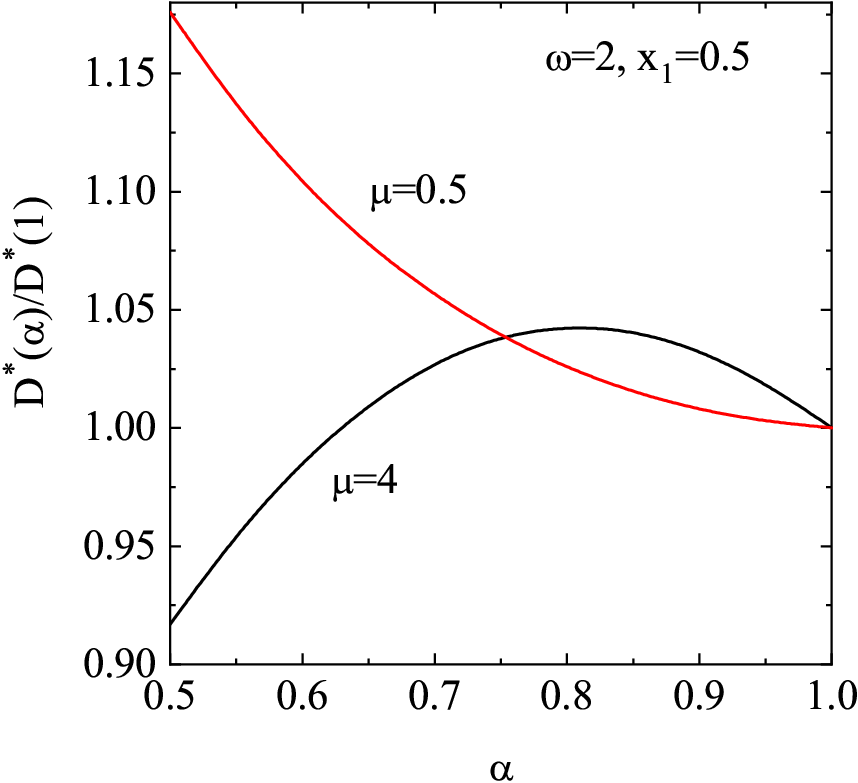
Given that the most interesting feature in a granular mixture is the dependence of the transport coefficients on inelasticity, we will normalize the values of the (dimensionless) transport coefficients with respect to their values for elastic collisions. Figures 1–3 show , , and as a function of for , , and two different values of the mass ratio : and . For elastic collisions, , and
| (108) |
where
| (109) |
The thermal diffusion coefficient has not been normalized with its value in the elastic limit because this coefficient vanishes for elastic collisions in the first Sonine approximation. Ferziger and Kaper 1972; KCLH87 Beyond the first Sonine solution, but its magnitude is very small. We observe that in general the effect of inelasticity on mass transport is significant since the (reduced) coefficients , , and clearly deviate from their forms for elastic collisions. However, these deviations are in general smaller than those obtained in the conventional IHS model (see for instance, Figs. 1-3 of Ref. Garzó, Montanero, and Dufty 2006). This feature was already previously noted in the monodisperse case. GBS18 With respect to the dependence on the mass ratio, we see that there is a monotonic decrease of the diffusion coefficients with decreasing , except for the scaled diffusion when since this coefficient exhibits in this case a non-monotonic dependence on inelasticity. Moreover, for sufficiently strong inelasticity (let’s say, ), the impact of the coefficient of restitution on mass transport increases as the mass of the small particle increases. Figure 3 also highlights that the thermal diffusion coefficient seems to be always positive, at least in the case illustrated here. This feature contrasts to what happens in the conventional IHS model where this coefficient can be negative (see for instance, Fig. 3 of Ref. Garzó, Montanero, and Dufty 2006). The signature of the coefficient is relevant in problems such as granular segregation by thermal diffusion. Jenkins and Yoon 2002; Brey, Ruiz-Montero, and Moreno 2005; Brey, Ruiz-Montero, and Moreno 2006; Serero et al. 2006; Garzó 2006; Garzó 2008; Brito et al. 2008; Garzó 2009; Garzó 2011
The ratio is plotted in Fig. 4 as a function of the coefficient of restitution . As before, refers to the shear viscosity coefficient for elastic collisions. As occurs in the case of the diffusion coefficients, we observe that the effect of inelasticity on the shear viscosity is less important than in the conventional IHS model (see for instance, Fig. 5 of Ref. Garzó and Montanero 2007). In addition, depending on the mass ratio, the normalized shear viscosity decreases (increases) when decreasing when the mass ratio is larger (smaller) than 1. The (reduced) coefficients and are plotted in Figs. 5 and 6, respectively. We recall here that in the conventional IHS model. First, as expected, both coefficients vanish for elastic collisions. However, as inelasticity increases, the magnitude of both coefficients is not negligible. This means that and should be considered when one would solve the corresponding Navier–Stokes hydrodynamic equations. At a given value of , while increases with decreasing , increases (decreases) with inelasticity when (). This means that for the considered case of equal and , is always positive (negative) when the mass ratio is smaller (larger) than 1.
VI Onsager’s reciprocal relations
Explicit knowledge of the Navier–Stokes transport coefficients for the -model of granular binary mixtures opens the possibility of several interesting applications. Among them, the quantification of the (possible) violation of the Onsager reciprocal relations is likely one of the most simple applications. This problem was already studied in the case of the conventional smooth IHS model. Garzó, Montanero, and Dufty 2006 Since time reversal symmetry is broken in granular gases (because collisions are inelastic), it is expected that Onsager’s relations fail for finite degree of inelasticity. On the other hand, we think that the assessment of the expected violation and the influence of inelasticity on it is still an interesting problem.


In the usual language of the linear irreversible thermodynamics for ordinary fluids, the constitutive equations for the mass flux (56) and heat flow (58) of a binary mixture are written as de Groot and Mazur 1984
| (110) |
| (111) | |||||
where is the chemical potential of the component . In the low-density regime,
| (112) |
The coefficients are the so-called Onsager phenomenological coefficients. For ordinary or molecular fluids (), Onsager showed that time reversal invariance of the underlying microscopic equations of motion leads to the restrictions:
| (113) |
The first two symmetries are called reciprocal relations as they relate transport coefficients for different processes. Thus, the coefficients link the mass flux to the thermal gradient while the coefficients link the heat flux to the gradient of the chemical potentials. The last two identities ( and ) are statements that the pressure gradient does not appear in any of the fluxes even though it is admitted by symmetry. In particular, the condition is important for monocomponent elastic gases since it yields Fourier’s law for heat flux () and hence, there is no any contribution proportional to the heat flux coming from the density gradient . On the contrary, for the IHS model, and there is an additional contribution to the heat flux proportional to . Soto, Mareschal, and Risso 1999; Brey et al. 1998; Garzó 2019
In order to analyze the violation of Onsager’s relations, one has first to express the Onsager coefficients (, , , , , and ) in terms of both the diffusion (, , ) and heat flux (, , ) transport coefficients. To make this connection, since , then Eq. (112) yields
| (114) |
The relationships between the Onsager coefficients and those appearing in Eqs. (56) and (58) are
| (115) |
| (116) |
| (117) |
| (118) |
| (119) |
As said before, since is symmetric under the change , then Onsager’s relation trivially holds. To analyze the other relations, we define the dimensionless function
| (120) | |||||
which vanishes when . Similarly,
| (121) |
vanishes when . Finally, when and , the function
| (122) |
equals zero.
For elastic collisions, and and are given by Eqs. (108) and (109); this leads to . Also, for mechanically equivalent particles with arbitrary , so that , , and vanish. However, beyond these limit cases, Onsager’s relations do not apply as expected. At this macroscopic level the origin of this failure is due to the homogeneous reference state [which gives contributions to diffusion coefficients coming from the derivatives and ] as well as the occurrence of different kinetic temperatures for both components (). Figure 7 shows the dependence of the quantities , , and on the (common) coefficient of restitution for mass ratios and . Violation of Onsager’s relations is especially relevant in the case of the function . We see that the departure from zero in the cases of and is very small even for strong dissipation, implying that and are small. In fact, the deviations from Onsager’s relations are significantly much smaller than those found in the IHS model for the same systems (see Figs. 7, 8, and 9 of Ref. Garzó, Montanero, and Dufty 2006).
VII Discussion
The present paper has been focused on the derivation of the Navier–Stokes hydrodynamic equations for a granular binary mixture of inelastic hard spheres in the context of the so-called -model. This model was originally proposed by Brito et al. Brito, Risso, and Soto 2013 to mimic the transfer of energy from the vertical to horizontal degrees of freedom in a quasi-two dimensional-dimensional geometry. Olafsen and Urbach 1998; Prevost et al. 2004; Melby et al. 2005; Clerc et al. 2008; Pacheco-Vázquez, Caballero-Robledo, and Ruiz-Suárez 2009; Rivas et al. 2011; Gradenigo et al. 2011; Castillo, Mújica, and Soto 2012; Puglisi et al. 2012 Beyond its possible connection with this sort of experiments, the -model can be also seen as a nice and reliable alternative to the use of external driving forces to achieve a nonequilibrium steady state in a granular gas when collisional cooling is compensated for by the injected energy.
Although this collisional model has been widely employed by several groups Brey et al. 2013; Brey et al. 2014; Brey et al. 2015; Brey et al. 2016; Soto, Risso, and Brito 2014; GBS18 for studying dynamic properties (kurtosis in homogeneous states, transport coefficients, ) for monocomponent granular gases, we are not aware of any previous attempt for extending the previous efforts to the interesting case of multicomponent granular gases, except for our previous analysis on the lack of equipartition in homogeneous binary mixtures. Brito, Soto, and Garzó 2020 Needless to say, the determination of the complete set of Navier–Stokes transport coefficients of granular mixtures is challenging not only from a fundamental point of view, but also from a more practical view since granular matter is usually presented in nature as a collection of particles of different sizes, shapes, masses, and/or coefficients of restitution. Thus, given the high number of parameters involved in the description of these systems, one usually considers simple systems to gain some insight. For this reason, the low-density regime has been considered here where the set of Boltzmann kinetic equations for the mixture provides an accurate framework for analyzing transport properties.
As in previous works on granular mixtures, Garzó and Dufty 2002; Garzó and Montanero 2007 the constitutive equations for the mass, momentum, and heat fluxes and the cooling rate have been obtained by solving the Boltzmann equation by means of the Chapman–Enskog expansion up to first order in the spatial gradients. The constitutive equation of the mass flux is given by Eq. (56) where the diffusion transport coefficients , , and are defined by Eqs. (59)–(61), respectively. The pressure tensor is given by Eq. (57) where the shear viscosity coefficient is defined by Eq. (62). The heat flux is given by Eq. (58) where the heat flux transport coefficients , , and are defined by Eqs. (63)–(65), respectively. Apart from the above transport coefficients, there are non-vanishing first-order contributions to the partial temperatures and the cooling rate ; they are given by Eqs. (66)–(67) and (92), respectively. This latter result contrasts with the one previously obtained in the conventional IHS model where at low-density. Garzó and Dufty 2002; Garzó and Montanero 2007
Explicit forms of the above transport coefficients have been obtained by considering the leading terms in a Sonine polynomial expansion of the first-order distribution function. This is the usual way for determining these quantities for elastic Chapman and Cowling 1970 and inelastic Garzó 2019 gases. On the other hand, given that the evaluation of the heat flux transport coefficients requires to consider the second Sonine approximation, here we have addressed the computation of the diffusion transport coefficients, the shear viscosity, and the quantities , and . In the general time-dependent problem, the differential equations obeying the diffusion coefficients are given by Eqs. (73)–(75), the viscosity obeys Eq. (87), and the first-order contributions to the partial temperatures are given in terms of the solution of Eq. (95). The numerical solutions of the above differential equations provide the dependence of the transport coefficients on the parameter space of the system.
Considering that the zeroth-order distribution functions are involved in the evaluation of transport coefficients, one has to characterize first these distributions before computing transport. This study has been previously made in Ref. Brito, Soto, and Garzó 2020 where it has been shown that has the scaling form (44) and the temperature ratios obey the set of coupled equations (51). In the steady state (), the dependence of on the parameters of the mixture has been explicitly obtained by approximating the scaled distributions by Maxwellian distributions at [see Eq. (124)]. In spite of this approximation, the theoretical results for the temperature ratio compare quite well with computer simulations, specially for low-density mixtures. Brito, Soto, and Garzó 2020
Once the reference state is well characterized, the forms of the above set of transport coefficients under steady state conditions have been explicitly determined; their expressions have been displayed in Eqs. (104)–(103), (105), and (106). It is apparent that in general they exhibit a quite complex dependence on the coefficients of restitution and the remaining parameters of the mixture. An interesting point is that their expressions not only depend on the hydrodynamic fields in the steady state, but, in addition, there are contributions to them coming from the derivatives of both the temperature ratio and the cooling rate in the vicinity of the steady state. These contributions measure the distance of the perturbed state from the steady reference state. This sort of contributions are also present in the case of driven granular mixtures Khalil and Garzó 2013; Khalil and Garzó 2018; Gómez González, Khalil, and Garzó 2020 but they absent in the conventional IHS model for undriven granular mixtures. Garzó and Dufty 2002; Garzó and Montanero 2007; Garzó, Murray, and Vega Reyes 2013
To illustrate the dependence of transport on the (common) coefficient of restitution , the simplest case has been considered. Figures 1–6 highlights the significant effect of inelasticity on mass and momentum transport as well as on the partial temperatures. However, at a more quantitative level, the influence of on the transport coefficients is smaller than that of the conventional collisional model. Garzó and Dufty 2002; Garzó and Montanero 2007; Garzó, Murray, and Vega Reyes 2013
It is well known that the hydrodynamic equations for granular mixtures are the same as for a molecular mixture, except for (i) a sink in the energy equation due to granular cooling, and (ii) additional transport coefficients in the mass and heat flux constitutive equations. These additional contributions arise because Onsager reciprocal relations de Groot and Mazur 1984 among various transport coefficients are expected to fail. Here, as an application of the previous results, we have assessed in Sec. VI the violation of Onsager’s relations as inelasticity increases. Notably, as Fig. 7 shows, the failure of these relations are much smaller than those reported in Ref. Garzó, Montanero, and Dufty 2006 for the same systems.
As mentioned in Sec. I, the -model was originally proposed to mimic the quasi-two-dimensional geometry of a confined granular gas .Olafsen and Urbach 1998; Prevost et al. 2004; Melby et al. 2005; Clerc et al. 2008; Pacheco-Vázquez, Caballero-Robledo, and Ruiz-Suárez 2009; Rivas et al. 2011; Castillo, Mújica, and Soto 2012 However, although this collisional model is able to describe quite well Brey et al. 2017 the homogeneous evolution observed in the experiments, it fails to predict the existence of non-equilibrium phase transitions. For this reason, modified Boltzmann kinetic equations for this special quasi-two-dimensional confinement have been proposed Brey, Maynar, and García de Soria 2016; Risso, Soto, and Guzmán 2018 and the inhomogeneous cooling state has been widely analyzed. Brey, García de Soria, and Maynar 2019; Maynar, García de Soria, and Brey 2019; Maynar, García de Soria, and Brey 2019
On the other hand, there are still some interesting open problems in the -model. Among them, the evaluation of the heat flux transport coefficients by considering the second Sonine approximation is a challenging issue. The knowledge of these coefficients will allow us to perform a linear stability analysis of the homogeneous steady state. A previous study for monocomponent gases Brey et al. 2016 has shown the stability of the homogeneous state for small spatial perturbations and it is relevant to determine if the stability of the homogeneous steady state is extended for granular mixtures. Moreover, given that most of the theoretical results found here have been obtained under certain approximations (Maxwellian distribution functions for the reference states , leading Sonine approximations for the diffusion transport coefficients and the shear viscosity), a natural project is to undertake simulations to gauge the reliability of the present results. In particular, we plan to carry out computer simulations to measure the tracer diffusion coefficient (namely, a binary mixture where the concentration of one of the components is negligible) in a similar way as those simulations performed in the conventional IHS model. Brey et al. 2000; Garzó and Vega Reyes 2009; Garzó and Vega Reyes 2012 An additional challenging problem is to measure the Navier–Stokes shear viscosity by studying the decay of a small perturbation to the transversal component of the velocity field. Brey, Ruiz-Montero, and Cubero 1999 Finally, another possible project for the next future is to analyze thermal diffusion segregation. Garzó 2008; Brito et al. 2008; Garzó 2009; Garzó 2011 Works on the above issues will be developed in the near future.
Acknowledgements.
The research of V.G. has been supported by the Spanish Ministerio de Economía y Competitividad through Grant No. FIS2016-76359-P and by the Junta de Extremadura (Spain) Grant Nos. IB16013 and GR18079, partially financed by “Fondo Europeo de Desarrollo Regional” funds. The work of R.B. has been supported by the Spanish Ministerio de Economía y Competitividad through Grant No. FIS2017-83709-R. The research of R.S. has been supported by the Fondecyt Grant No. 1180791 of ANID (Chile).Appendix A Derivatives of the temperature ratio in the vicinity of the steady state
In this Appendix, the derivatives of the temperature ratio with respect to , , , and in the vicinity of the steady state are evaluated. The derivatives of can be easily obtained by taking into account the relation .
Let us consider first the derivative of with respect to . To determine it, we consider Eq. (52) for :
| (123) |
The (reduced) partial cooling rates are functionals of the (scaled) distributions and whose exact forms are not known. However, recent results Brito, Soto, and Garzó 2020 have clearly shown that the quantities can be well estimated by using Maxwellian distributions at different temperatures. This is justified by the good agreement found between theory (based on the above assumption) and simulations for the global temperature and the temperature ratio even for strong dissipation and/or disparate values of the mass and size ratios. Thus, to estimate we consider the approximation
| (124) |
In the Maxwellian approximation (124), the cooling rate is Brito, Soto, and Garzó 2020
| (125) | |||||
where . The expression of can be obtained from Eq. (125) by making the change . The total cooling rate is given by , where use has been made of the relation . In the steady state, and hence, Eq. (123) is trivially verified. To determine the derivative at the steady state, we take first the derivative with respect to in both sides of Eq. (123) and then take the steady-state limit. After some algebra, one gets the result
| (126) |
where the subscript means that all the quantities are evaluated in the steady state. According to Eq. (125), depends on explicitly and also through its dependence on . Thus,
| (127) |
Equations defining the remaining derivatives and can be easily obtained by following identical steps. They are given
| (128) |
| (129) |
The solution to the set of algebraic nonlinear equations (126), (128), and (129) provides the derivatives , , and at the steady state. A more simple expression can be obtained for the particular case . In this situation, it is easy to see that the derivative obeys the following quadratic equation:
| (130) |
where
| (131) |
An analysis of the solutions to Eq. (130) shows that in general one of the roots leads to unphysical behavior of the diffusion coefficients for nearly elastic spheres. We take the other root as the physical root of the quadratic equation.
Appendix B Some technical details on the first-order Chapman–Enskog solution
To first order in the gradients, the equation for is
| (133) |
where . In Eq. (133) it is understood that and the linear operators and are
| (134) |
| (135) |
The action of the time derivatives on the hydrodynamic fields is
| (136) |
where use has been made of the results . Here, is the first-order contribution to the cooling rate. The right-hand side of Eq. (133) can be explicitly evaluated from the relations (136) with the result
| (137) |
The kinetic equation for can be easily written when one takes into account Eq. (137):
| (138) | |||||
The coefficients of the field gradients on the right side are functions of and the hydrodynamic fields. They are given by
| (139) |
| (140) |
| (141) |
Note that that is given in terms of the unknown distribution function . In addition, since is a scalar then it must be proportional to since , , and are vectors and the tensor is a traceless tensor. Therefore, the term can be written as
| (142) |
and Eq. (138) reads
| (143) | |||||
where
| (144) |
Upon obtaining Eq. (144) use has been made of the relations (45) and (46).
The solution to Eq. (138) is of the form
| (145) |
The coefficients , , , , and are functions of the peculiar velocity and the hydrodynamic fields. The cooling rate depends on space through its dependence on , , and . The time derivative acting on these quantities can be evaluated by the replacement . In addition, there are contributions coming from the action of the operator on the temperature and pressure gradients given by
| (146) | |||||
| (147) | |||||
where we recall that and .
The integral equations for , , , , and are identified as coefficients of the independent gradients in Eq. (138):
| (148) |
| (149) |
| (150) |
| (151) |
| (152) |
In Eqs. (148)–(152), as said before, it is understood that .
Since is coupled with the unknowns , its explicit form can be identified after expanding the expression (15) of the cooling rate to first order in spatial gradients. After some algebra, can be written as , where
| (153) |
| (154) | |||||
Here, and
| (155) |
Appendix C Collision frequencies , , and
In this Appendix, we give some technical details for the evaluation of the collision frequencies , , and . To obtain them, the property (II.2) is used. Let us consider first . According to Eqs. (1)–(2) and (II.2), the quantity can be split in two parts: one of them already computed in the conventional IHS model (i.e., when ) and the other part involving terms proportional to . Thus, the collision frequency reads
| (156) |
where was determined in Ref. Garzó and Montanero 2007 and its expression is
| (157) |
The quantity is
| (158) |
where use has been made of the result
| (159) |
To integrate over and in Eq. (158) we substitute the zeroth-order distributions () by their Maxwellian distributions defined by Eq. (69). With these replacements, is finally given by
| (160) |
The expression (IV.1) for can be easily obtained from Eqs. (157) and (160).
The collision frequencies and are defined by Eqs. (88) and (89), respectively. To obtain them, as before, we replace by its Maxwellian distribution . As in the case of , the forms of and can be written as
| (161) |
where the contributions and (i.e., when ) are Garzó and Montanero 2007
| (162) | |||||
| (163) | |||||
The evaluation of and follows similar mathematical steps as those made in the evaluation of . Only the final expressions are provided here. They are given by
| (164) | |||||
| (165) |
The expressions of and can be easily inferred from Eqs. (162)–(165) by making the change . In the case of mechanically equivalent particles (, , , and ), Eqs. (164) and (165) yield
| (166) |
This result is consistent with the one previously found for monocomponent granular gases in the -model. Brey et al. 2015
Finally, the expressions of the collision frequencies and are
| (167) | |||||
| (168) | |||||
As before, the expressions of and can be easily obtained from Eqs. (167) and (168), respectively, by making the change .
DATA AVAILABILITY
The data that support the findings of this study are available from the corresponding author upon reasonable request.
References
- Brilliantov and Pöschel (2004) N. Brilliantov and T. Pöschel, Kinetic Theory of Granular Gases (Oxford University Press, Oxford, 2004).
- Garzó (2019) V. Garzó, Granular Gaseous Flows (Springer Nature, Cham, 2019).
- Yang et al. (2002) X. Yang, C. Huan, D. Candela, R. W. Mair, and R. L. Walsworth, “Measurements of grain motion in a dense, three-dimensional granular fluid,” Phys. Rev. Lett. 88, 044301 (2002).
- Huan et al. (2004) C. Huan, X. Yang, D. Candela, R. W. Mair, and R. L. Walsworth, “NMR experiments on a three-dimensional vibrofluidized granular medium,” Phys. Rev. E 69, 041302 (2004).
- Abate and Durian (2006) A. R. Abate and D. J. Durian, “Approach to jamming in an air-fluidized granular bed,” Phys. Rev. E 74, 031308 (2006).
- Schröter, Goldman, and Swinney (2005) M. Schröter, D. I. Goldman, and H. L. Swinney, “Stationary state volume fluctuations in a granular medium,” Phys. Rev. E 71, 030301(R) (2005).
- Puglisi et al. (1999) A. Puglisi, V. Loreto, U. M. B. Marconi, and A. Vulpiani, “Kinetic approach to granular gases,” Phys. Rev. E 59, 5582–5595 (1999).
- Cafiero, Luding, and Herrmann (2000) R. Cafiero, S. Luding, and H. J. Herrmann, “Two-dimensional granular gas of inelastic spheres with multiplicative driving,” Phys. Rev. Lett. 84, 6014–6017 (2000).
- Prevost, Egolf, and Urbach (2002) A. Prevost, D. A. Egolf, and J. S. Urbach, “Forcing and velocity correlations in a vibrated granular monolayer,” Phys. Rev. Lett. 89, 084301 (2002).
- Paganobarraga et al. (2002) I. Paganobarraga, E. Trizac, T. P. C. van Noije, and M. H. Ernst, “Randomly driven granular fluids: Collisional statistics and short scale structure,” Phys. Rev. E 65, 011303 (2002).
- Puglisi, Baldassarri, and Loreto (2002) A. Puglisi, A. Baldassarri, and V. Loreto, “Fluctuation-dissipation relations in driven granular gases,” Phys. Rev. E 66, 061305 (2002).
- Fiege, Aspelmeier, and Zippelius (2009) A. Fiege, T. Aspelmeier, and A. Zippelius, “Long-time tails and cage effect in driven granular fluids,” Phys. Rev. Lett. 102, 098001 (2009).
- Kranz, Sperl, and Zippelius (2010) W. T. Kranz, M. Sperl, and A. Zippelius, “Glass transition for driven granular fluids,” Phys. Rev. Lett. 104, 225701 (2010).
- Vollmayr-Lee, Aspelmeier, and Zippelius (2011) K. Vollmayr-Lee, T. Aspelmeier, and A. Zippelius, “Hydrodynamic correlation functions of a driven granular fluid in steady state,” Phys. Rev. E 83, 011301 (2011).
- Gradenigo et al. (2011) G. Gradenigo, A. Sarracino, D. Villamaina, and A. Puglisi, “Non-equilibrium length in granular fluids: From experiment to fluctuating hydrodynamics,” Europhys. Lett. 96, 14004 (2011).
- Puglisi et al. (2012) A. Puglisi, A. Gnoli, G. Gradenigo, A. Sarracino, and D. Villamaina, “Structure factors in granular experiments with homogeneous fluidization,” J. Chem. Phys. 136, 014704 (2012).
- Brey et al. (1998) J. J. Brey, J. W. Dufty, C. S. Kim, and A. Santos, “Hydrodynamics for granular flows at low density,” Phys. Rev. E 58, 4638–4653 (1998).
- Santos, Garzó, and Dufty (2004) A. Santos, V. Garzó, and J. W. Dufty, “Inherent rheology of a granular fluid in uniform shear flow,” Phys. Rev. E 69, 061303 (2004).
- Cordero, Risso, and Soto (2005) P. Cordero, D. Risso, and R. Soto, “Steady quasi-homogeneous granular gas state,” Physica A 356, 54–60 (2005).
- Olafsen and Urbach (1998) J. S. Olafsen and J. S. Urbach, “Clustering, order, and collapse in a driven granular monolayer,” Phys. Rev. Lett. 81, 4369–4372 (1998).
- Prevost et al. (2004) A. Prevost, P. Melby, D. A. Egolf, and J. S. Urbach, “Nonequilibrium two-phase coexistence in a confined granular layer,” Phys. Rev. E 70, 050301(R) (2004).
- Melby et al. (2005) P. Melby, F. Vega Reyes, A. Prevost, R. Robertson, P. Kumar, D. A. Egolf, and J. S. Urbach, “The dynamics of thin vibrated granular layers,” J. Phys. C: Condens. Matter 17, S2689 (2005).
- Clerc et al. (2008) M. G. Clerc, P. Cordero, J. Dunstan, K. Huff, N. Mujica, D. Risso, and G. Varas, “Liquid-solid-like transition in quasi-one-dimensional driven granular media,” Nature Phys. 4, 249 (2008).
- Pacheco-Vázquez, Caballero-Robledo, and Ruiz-Suárez (2009) F. Pacheco-Vázquez, G. A. Caballero-Robledo, and J. C. Ruiz-Suárez, “Superheating in granular matter,” Phys. Rev. Lett. 102, 170601 (2009).
- Rivas et al. (2011) N. Rivas, S. Ponce, B. Gallet, D. Risso, R. Soto, P. Cordero, and N. Mújica, “Sudden chain energy transfer events in vibrated granular media,” Phys. Rev. Lett. 106, 088001 (2011).
- Castillo, Mújica, and Soto (2012) G. Castillo, N. Mújica, and R. Soto, “Fluctuations and criticality of a granular solid-liquid-like phase transition,” Phys. Rev. Lett. 109, 095701 (2012).
- Mujica and Soto (2016) N. Mujica and R. Soto, “Dynamics of noncohesive confined granular media,” in Recent Advances in Fluid Dynamics with Environmental Applications (Springer, 2016) pp. 445–463.
- Brito, Risso, and Soto (2013) R. Brito, D. Risso, and R. Soto, “Hydrodynamic modes in a confined granular fluid,” Phys. Rev. E 87, 022209 (2013).
- Maynar, García de Soria, and Brey (2019) P. Maynar, I. García de Soria, and J. J. Brey, “Homogeneous dynamics in a vibrated granular monolayer,” J. Stat. Mech. 093205 (2019).
- Risso, Soto, and Guzmán (2018) D. Risso, R. Soto, and R. Guzmán, “Effective two-dimensional model for granular matter with phase separation,” Phys. Rev. E 98, 022901 (2018).
- Brey et al. (2013) J. J. Brey, M. I. García de Soria, P. Maynar, and V. Buzón, “Homogeneous steady state of a confined granular gas,” Phys. Rev. E 88, 062205 (2013).
- Brey et al. (2014) J. J. Brey, P. Maynar, M. I. García de Soria, and V. Buzón, “Homogeneous hydrodynamics of a collisional model of confined granular gases,” Phys. Rev. E 89, 052209 (2014).
- Brey et al. (2015) J. J. Brey, V. Buzón, P. Maynar, and M. García de Soria, “Hydrodynamics for a model of a confined quasi-two-dimensional granular gas,” Phys. Rev. E 91, 052201 (2015).
- Brey et al. (2016) J. J. Brey, V. Buzón, M. I. García de Soria, and P. Maynar, “Stability analysis of the homogeneous hydrodynamics of a model for a confined granular gas,” Phys. Rev. E 93, 062907 (2016).
- Soto, Risso, and Brito (2014) R. Soto, D. Risso, and R. Brito, “Shear viscosity of a model for confined granular media,” Phys. Rev. E 90, 062204 (2014).
- (36) V. Garzó, R. Brito, and R. Soto, “Enskog kinetic theory for a model of a confined quasi-two-dimensional granular fluid,” Phys. Rev. E 98, 052904 (2018) [Erratum] Phys. Rev. E 102, 05901 (2020).
- Brito, Soto, and Garzó (2020) R. Brito, R. Soto, and V. Garzó, “Energy nonequipartition in a collisional model of a confined quasi-two-dimensional granular mixture,” arXiv:2009.02957 (2020).
- Garzó and Dufty (2002) V. Garzó and J. W. Dufty, “Hydrodynamics for a granular binary mixture at low density,” Phys. Fluids. 14, 1476–1490 (2002).
- Garzó, Montanero, and Dufty (2006) V. Garzó, J. M. Montanero, and J. W. Dufty, “Mass and heat fluxes for a binary granular mixture at low density,” Phys. Fluids 18, 083305 (2006).
- Serero et al. (2006) D. Serero, I. Goldhirsch, S. H. Noskowicz, and M. L. Tan, “Hydrodynamics of granular gases and granular gas mixtures,” J. Fluid Mech. 554, 237–258 (2006).
- Garzó and Montanero (2007) V. Garzó and J. M. Montanero, “Navier–Stokes transport coefficients of -dimensional granular binary mixtures at low-density,” J. Stat. Phys. 129, 27–58 (2007).
- Serero et al. (2009) D. Serero, S. H. Noskowicz, M. L. Tan, and I. Goldhirsch, “Binary granular gas mixtures: Theory, layering effects and some open questions,” Eur. Phys. J. Special Topics 179, 221–247 (2009).
- Garzó, Murray, and Vega Reyes (2013) V. Garzó, J. A. Murray, and F. Vega Reyes, “Diffusion transport coefficients for granular binary mixtures at low density: Thermal diffusion segregation,” Phys. Fluids 25, 043302 (2013).
- Chapman and Cowling (1970) S. Chapman and T. G. Cowling, The Mathematical Theory of Nonuniform Gases (Cambridge University Press, Cambridge, 1970).
- Karkheck and Stell (1979) J. Karkheck and G. Stell, “Bulk viscosity of fluid mixtures,” J. Chem. Phys. 71, 3636–3639 (1979).
- Gómez González and Garzó (2019) R. Gómez González and V. Garzó, “Influence of the first-order contributions to the partial temperatures on transport properties in polydisperse dense granular mixtures,” Phys. Rev. E 100, 032904 (2019).
- Lutsko (2004) J. F. Lutsko, “Kinetic theory and hydrodynamics of dense, reacting fluids far from equilibrium,” J. Chem. Phys. 120, 6325 (2004).
- Ferziger and Kaper (1972) J. H. Ferziger and G. H. Kaper, Mathematical Theory of Transport Processes in Gases (North-Holland, Amsterdam, 1972).
- Garzó and Santos (2003) V. Garzó and A. Santos, Kinetic Theory of Gases in Shear Flows. Nonlinear Transport (Kluwer Academic Publishers, Dordrecht, 2003).
- (50) R. Soto, Kinetic Theory and Transport Phenomena, Vol. 25 (Oxford University Press, Oxford, 2016).
- Garzó and Dufty (1999) V. Garzó and J. W. Dufty, “Homogeneous cooling state for a granular mixture,” Phys. Rev. E 60, 5706–5713 (1999).
- Brey, Ruiz-Montero, and Cubero (1999) J. J. Brey, M. J. Ruiz-Montero, and D. Cubero, “On the validity of linear hydrodynamics for low-density granular flows described by the Boltzmann equation,” Europhys. Lett. 48, 359–364 (1999).
- Brey et al. (2000) J. J. Brey, M. J. Ruiz-Montero, D. Cubero, and R. García-Rojo, “Self-diffusion in freely evolving granular gases,” Phys. Fluids. 12, 876–883 (2000).
- Brey, Ruiz-Montero, and Moreno (2001) J. J. Brey, M. J. Ruiz-Montero, and F. Moreno, “Hydrodynamics of an open vibrated granular system,” Phys. Rev. E 63, 061305 (2001).
- Dahl et al. (2002) S. R. Dahl, C. M. Hrenya, V. Garzó, and J. W. Dufty, “Kinetic temperatures for a granular mixture,” Phys. Rev. E 66, 041301 (2002).
- Lutsko, Brey, and Dufty (2002) J. F. Lutsko, J. J. Brey, and J. W. Dufty, “Diffusion in a granular fluid. II. Simulation,” Phys. Rev. E 65, 051304 (2002).
- Montanero and Garzó (2002) J. M. Montanero and V. Garzó, “Monte Carlo simulation of the homogeneous cooling state for a granular mixture,” Granular Matter 4, 17–24 (2002).
- Montanero and Garzó (2003) J. M. Montanero and V. Garzó, “Shear viscosity for a heated granular binary mixture at low density,” Phys. Rev. E 67, 021308 (2003).
- Garzó and Montanero (2003) V. Garzó and J. M. Montanero, “Shear viscosity for a moderately dense granular binary mixture,” Phys. Rev. E 68, 041302 (2003).
- Brey, Ruiz-Montero, and Moreno (2005) J. J. Brey, M. J. Ruiz-Montero, and F. Moreno, “Energy partition and segregation for an intruder in a vibrated granular system under gravity,” Phys. Rev. Lett. 95, 098001 (2005).
- Lois, Lemaître, and Carlson (2007) G. Lois, A. Lemaître, and J. M. Carlson, “Spatial force correlations in granular shear flow. II. Theoretical implications,” Phys. Rev. E 76, 021303 (2007).
- Mitrano et al. (2011) P. P. Mitrano, S. R. Dhal, D. J. Cromer, M. S. Pacella, and C. M. Hrenya, “Instabilities in the homogeneous cooling of a granular gas: a quantitative assessment of kinetic-theory predictions,” Phys. Fluids 23, 093303 (2011).
- Brey and Ruiz-Montero (2013) J. J. Brey and M. J. Ruiz-Montero, “Shearing instability of a dilute granular mixture,” Phys. Rev. E 87, 022210 (2013).
- Mitrano, Garzó, and Hrenya (2014) P. P. Mitrano, V. Garzó, and C. M. Hrenya, “Instabilities in granular binary mixtures at moderate densities,” Phys. Rev. E 89, 020201(R) (2014).
- (65) In standard textbooks like Ref. 44, a factor is usually assigned to the Boltzmann collision operator so that the operators and are formally of order . In this scheme, the operator is the same as our operator of Eqs. (3.8)–(3.10) The results derived from both formulations are of course completely equivalent for elastic collisions.
- (66) As discussed in Ref. 39, strictly speaking the thermal conductivity in a mixture is generally measured in the absence of diffusion (i.e., when ). To identify this coefficient, we have to express the heat flow in terms of , , and . The corresponding coefficient of defines the thermal conductivity coefficient.
- (67) J. M. Kincaid, E. G. D. Cohen, and M. López de Haro, “The Enskog theory for multicomponent mixtures. IV. Thermal diffusion”J. Chem. Phys. 86, 963–975 (1987).
- Jenkins and Yoon (2002) J. T. Jenkins and D. K. Yoon, “Segregation in binary mixtures under gravity,” Phys. Rev. Lett. 88, 194301 (2002).
- Brey, Ruiz-Montero, and Moreno (2006) J. J. Brey, M. J. Ruiz-Montero, and F. Moreno, “Hydrodynamic profiles for an impurity in an open vibrated granular gas,” Phys. Rev. E 73, 031301 (2006).
- Garzó (2006) V. Garzó, “Segregation in granular binary mixtures: Thermal diffusion,” Europhys. Lett. 75, 521–527 (2006).
- Garzó (2008) V. Garzó, “Brazil-nut effect versus reverse Brazil-nut effect in a moderately granular dense gas,” Phys. Rev. E 78, 020301 (R) (2008).
- Brito et al. (2008) R. Brito, H. Enríquez, S. Godoy, and R. Soto, “Segregation induced by inelasticity in a vibrofluidized granular mixture,” Phys. Rev. E 77, 061301 (2008).
- Garzó (2009) V. Garzó, “Segregation by thermal diffusion in moderately dense granular mixtures,” Eur. Phys. J. E 29, 261–274 (2009).
- Garzó (2011) V. Garzó, “Thermal diffusion segregation in granular binary mixtures described by the Enskog equation,” New J. Phys. 13, 055020 (2011).
- de Groot and Mazur (1984) S. R. de Groot and P. Mazur, Nonequilibrium Thermodynamics (Dover, New York, 1984).
- Soto, Mareschal, and Risso (1999) R. Soto, M. Mareschal, and D. Risso, “Departure from Fourier’s law for fluidized granular media,” Phys. Rev. Lett. 83, 5003 (1999).
- Khalil and Garzó (2013) N. Khalil and V. Garzó, “Transport coefficients for driven granular mixtures at low-density,” Phys. Rev. E 88, 052201 (2013).
- Khalil and Garzó (2018) N. Khalil and V. Garzó, “Heat flux of driven granular mixtures at low density: Stability analysis of the homogeneous steady state,” Phys. Rev. E 97, 022902 (2018).
- Gómez González, Khalil, and Garzó (2020) R. Gómez González, N. Khalil, and V. Garzó, “Enskog kinetic theory for multicomponent granular suspensions,” Phys. Rev. E 101, 012904 (2020).
- Brey et al. (2017) J. J. Brey, V. Buzón, P. Maynar, and M. I. García de Soria, “Kinetic theory of a confined quasi-two-dimensional gas of hard spheres,” Entropy 19, 68 (2017).
- Brey, Maynar, and García de Soria (2016) J. J. Brey, P. Maynar, and M. I. García de Soria, “Kinetic equation and non-equilibrium entropy for a quasi-two-dimensional gas,” Phys. Rev. E 94, 040103 (R) (2016).
- Brey, García de Soria, and Maynar (2019) J. J. Brey, M. I. García de Soria, and P. Maynar, “Inhomogeneous cooling state of a strongly confined granular gas at low density,” Phys. Rev. E 100, 052901 (2019).
- Maynar, García de Soria, and Brey (2019) P. Maynar, M. I. García de Soria, and J. J. Brey, “Understanding an instability in vibrated granular monolayers,” Phys. Rev. E 99, 032903 (2019).
- Garzó and Vega Reyes (2009) V. Garzó and F. Vega Reyes, “Mass transport of impurities in a moderately dense granular gas,” Phys. Rev. E 79, 041303 (2009).
- Garzó and Vega Reyes (2012) V. Garzó and F. Vega Reyes, “Segregation of an intruder in a heated granular gas,” Phys. Rev. E 85, 021308 (2012).