Distribution of Si II $\lambda$6355 Velocities of Type Ia Supernovae and Implications for Asymmetric Explosions2020Distribution of Si II $\lambda$6355 Velocities of Type Ia Supernovae and Implications for Asymmetric Explosions–References

The ML method requires the assumption that each observation $x$ comes from an underlying population distribution modeled as a probability density function $g(x,p_{1},\ldots,p_{m})$, where $p_{1},\ldots,p_{m}$ are parameters in the probability density function. Having $N$ observations of $x$, we assume each observation $x$ is independently sampled from identical distributions. Therefore, the chance of obtaining all $N$ observations is given by the function called the likelihood function,

The ML procedure maximises the log-likelihood $L_{\text{max}}$ for all possible values of the parameter ${p_{1},\ldots,p_{m}}$ determined by some defined parameter space. Since the logarithmic function is monotonic, the log-likelihood function reaches maximum where the likelihood function does as well.

Since the likelihood is the chance of an observation under some hypothesis of the underlying population, if there are two hypotheses, the ratio of two likelihoods (called the likelihood ratio) states how likely one hypothesis is compared to the other. The likelihood ratio is better interpreted using the likelihood ratio $\chi^{2}$ statistics (not to be confused with the Pearson’s $\chi^{2}$ statistics as introduced in the previous section),

In our case, the observable variable $x$ is the Si II $\lambda$6355 velocity $v$. We take the hypothesis that $v$ is distributed normally; more specifically, it is distributed as the sum of $k$ normal components, where the components have the functional form

To find the maximum of $L_{k}$, we adopt SciPy’s implementation of Nelder-Mead optimisation, scipy.optimize²² 2 https://docs.scipy.org/doc/scipy/reference/optimize.html, in Python 3 to determine the argmax simultaneously for each of the parameters $\mu_{l}$, $\sigma_{l}$, and $w_{l}$. We start with only one normal component ($k=1$) and find $L_{\mathrm{1,max}}=-2683$. We then add another normal component ($k=2$) and find $L_{\mathrm{2,max}}=-2648$, statistically significantly higher than $L_{\mathrm{1,max}}$, which is a strong argument that two-component fitting is better than one-component fitting (see below for a more detailed discussion about the statistical improvement). We also try to adopt a third normal component, but the optimisation program was not able to converge and the resulting log-likelihood does not significantly differ from the results of using two components. This indicates that a third component is not needed for the fitting. We thus focus our discussion on the one- and two-component cases.

In Table 1, we list the best estimated parameters for the one- and two-component cases and plot the results in Figure 3. In the one-component case, we find best-estimated parameters of $\mu_{1}=$11,500\text{\,}\mathrm{km}\text{\,}{\mathrm{s}}^{-1}$$ and $\sigma_{1}=$1300\text{\,}\mathrm{km}\text{\,}{\mathrm{s}}^{-1}$$ with $w_{1}$ fixed to be 311 (shown as the black dotted line in Figure 3). The two-component case consists of a group of SNe Ia with a lower and narrower-scatter velocity ($\mu_{1}=$11,000\text{\,}\mathrm{km}\text{\,}{\mathrm{s}}^{-1}$$, $\sigma_{1}=$700\text{\,}\mathrm{km}\text{\,}{\mathrm{s}}^{-1}$$, and $w_{1}=201$, shown as a blue dot-dashed line in Figure 3), and another group of SNe Ia with a higher and broader-scatter velocity ($\mu_{2}=$12,300\text{\,}\mathrm{km}\text{\,}{\mathrm{s}}^{-1}$$, $\sigma_{2}=$1800\text{\,}\mathrm{km}\text{\,}{\mathrm{s}}^{-1}$$, and $w_{2}=110$, shown as a red dashed line in Figure 3). The combination of the two groups is illustrated with a black solid line in Figure 3. Our results are similar to those of Wang et al. 2013, who reported a lower velocity with $\mu_{1}=$10,800\text{\,}\mathrm{km}\text{\,}{\mathrm{s}}^{-1}$$ and a higher velocity with $\mu_{2}=$13,000\text{\,}\mathrm{km}\text{\,}{\mathrm{s}}^{-1}$$ (no scatter values were reported).

For comparison, we also use the least-squares binned fitting method scored by the Pearson’s $\chi^{2}$ statistic to fit the histogram distribution of Si II $\lambda$6355 velocities with one and two normal components. The data are binned into 9 bins with width $500\text{\,}\mathrm{km}\text{\,}{\mathrm{s}}^{-1}$, where bin 1 is $v\leq$9500\text{\,}\mathrm{km}\text{\,}{\mathrm{s}}^{-1}$$ and bin 9 is $v>$13,000\text{\,}\mathrm{km}\text{\,}{\mathrm{s}}^{-1}$$. The bins were chosen purposefully so that each bin has at least an expected count of 4. The fitting results are also listed in Table 1; we see that the best-fit parameters from the $\chi^{2}$ fitting are very close to those of the ML method. For the two-components case, the $\chi^{2}$ fitting also reveals that there is a lower velocity, narrower-scatter group and a higher velocity, broader scatter group, confirming the findings from the ML method. Note that since Pearson’s $\chi^{2}$ method has the disadvantage of depending on how one bins the data, we only adopt ML method result for further analysis.

To estimate the statistical improvement of the two-component fitting over the one-component fitting, we first look at the likelihood ratio $\chi^{2}$ statistics in the ML method according to Equation (3). We take the null hypothesis that the data are distributed as a unimodal normal $k=1$. The alternative hypothesis adds a new component — that is, moving from $k=1$ to $k=2$, the ML solution of $L_{\mathrm{1,max}}$ changes to $L_{\mathrm{2,max}}$. This also increases the number of free parameters by 3 ($w_{2}$, $\mu_{2}$, and $\sigma_{2})$. Applying Equation (3) to $L_{\mathrm{2,max}}$ and $L_{\mathrm{1,max}}$, we find that the likelihood ratio $\chi^{2}$ statistic is 70 with 3 degrees of freedom. The $p$-value calculated from the $\chi^{2}$ statistic is much less than 0.01; hence, the improvement of the two-component model over the one-component model is statistically significant.

As an independent check, we also adopt the Akaike Information Criterion (AIC; Akaike 1974) to apply a penalty according to the number of free parameters to prevent overfitting. The AIC makes it possible to perform model selection when the models have different numbers of free parameters. To be sensitive to the sampling error of a small dataset, we use the modified version of AIC denoted as AICc (Sugiura 1978),

In conclusion, both the likelihood ratio test and the AICc test show strong statistical improvements for $k=2$ fitting than $k=1$ fitting. Therefore, if the velocity distribution is distributed normally (i.e., Gaussian mixture models), then the observed velocity is best described as two independent Gaussian distributions (Group I and Group II): one group with lower, narrower-scatter velocity ($\mu_{1}=$11,000\text{\,}\mathrm{km}\text{\,}{\mathrm{s}}^{-1}$$, $\sigma_{1}=$700\text{\,}\mathrm{km}\text{\,}{\mathrm{s}}^{-1}$$) and another group with higher, broader-scatter velocity ($\mu_{2}=$12,300\text{\,}\mathrm{km}\text{\,}{\mathrm{s}}^{-1}$$, $\sigma_{2}=$1800\text{\,}\mathrm{km}\text{\,}{\mathrm{s}}^{-1}$$). The ratio of the two groups is 201:110 (corresponding to 65%:35%) in the number of samples from the weight parameters. This velocity distribution is henceforth called the bimodal Gaussian distribution.

As one can see from Figure 3 for the two-component result, the second group of SNe Ia, whose mean velocity is higher than that of the first group, also has greater scatter than the first group, so there is a large overlap with the first group on the low-velocity side (the high-velocity side is dominated by the second group). In fact, the low-velocity side from the second group extends even farther than the first group. We thus think it is inappropriate to name the first group as low-velocity SNe Ia and the second group as high-velocity SNe Ia. Instead, here we suggest naming the lower mean velocity group as “Group I" and the other group as “Group II."

Because of the large overlap between the two groups, it is difficult to assign a specific SN Ia with a given velocity to a specific group, especially if the velocity is in the range $9500\text{\,}\mathrm{km}\text{\,}{\mathrm{s}}^{-1}12,000\text{\,}\mathrm{km}\text{\,}{\mathrm{s}}^{-1}$. But for a velocity beyond that range, one can compare the probability between the two groups according to the probability distribution function assuming the Si II $\lambda$6355 velocity data came from independently sampling each (but be cautious because the observed SN counts in those ranges are small). For $v<$9500\text{\,}\mathrm{km}\text{\,}{\mathrm{s}}^{-1}$$, the probability ratio between Group I and Group II is 21%:79%; for $v>$12,000\text{\,}\mathrm{km}\text{\,}{\mathrm{s}}^{-1}$$, the ratio is 12%:88%. Furthermore, for $v>$ $13,000\text{\,}\mathrm{km}\text{\,}{\mathrm{s}}^{-1}$, the probability for being in Group II is $>99\%$, which means almost all SNe Ia with velocity $>$ $13,000\text{\,}\mathrm{km}\text{\,}{\mathrm{s}}^{-1}$ belong to Group II according to the fitting.

Before starting the simulation of the velocity distributions, we need to quantify the velocity changes as a function of the viewing angle due to the asymmetric ejecta. To do this, we use the model spectra synthesised at different viewing angles to measure the Si II $\lambda$6355 velocity. We adopt the synthesised spectra from two different models, one from Kasen & Plewa 2007 and the other from Townsley et al. 2019; these models provide spectra at the time of SN Ia peak brightness for different viewing angles. Note, however, that our simulation setups can be updated easily to adopt other models, if desired.

Kasen & Plewa 2007 studied in detail one model called Y12, selected from the detonating failed deflagration (DFD) scenario (Plewa 2007), which considers an off-center, mild ignition process in a degenerate Chandrasekhar-mass C-O white dwarf. In the Y12 model, the white dwarf is initially ignited within a small spherical region on the axis of symmetry, 50 km in size and offset 12.5 km from the center. A temporal series of synthetic spectra was calculated for different viewing angles; of particular interest to us are the spectra near the time of maximum brightness (see Fig. 7 of Kasen & Plewa 2007). In this model, the viewing angle was defined as $\theta=$$$ on the ignition side and $\theta=$$$ on the detonation side. We measure the Si II $\lambda$6355 velocity from the maximum-light synthetic spectra at different viewing angles (simply treating them as real spectra) and plot the results in Figure 4, shown as blue circles.

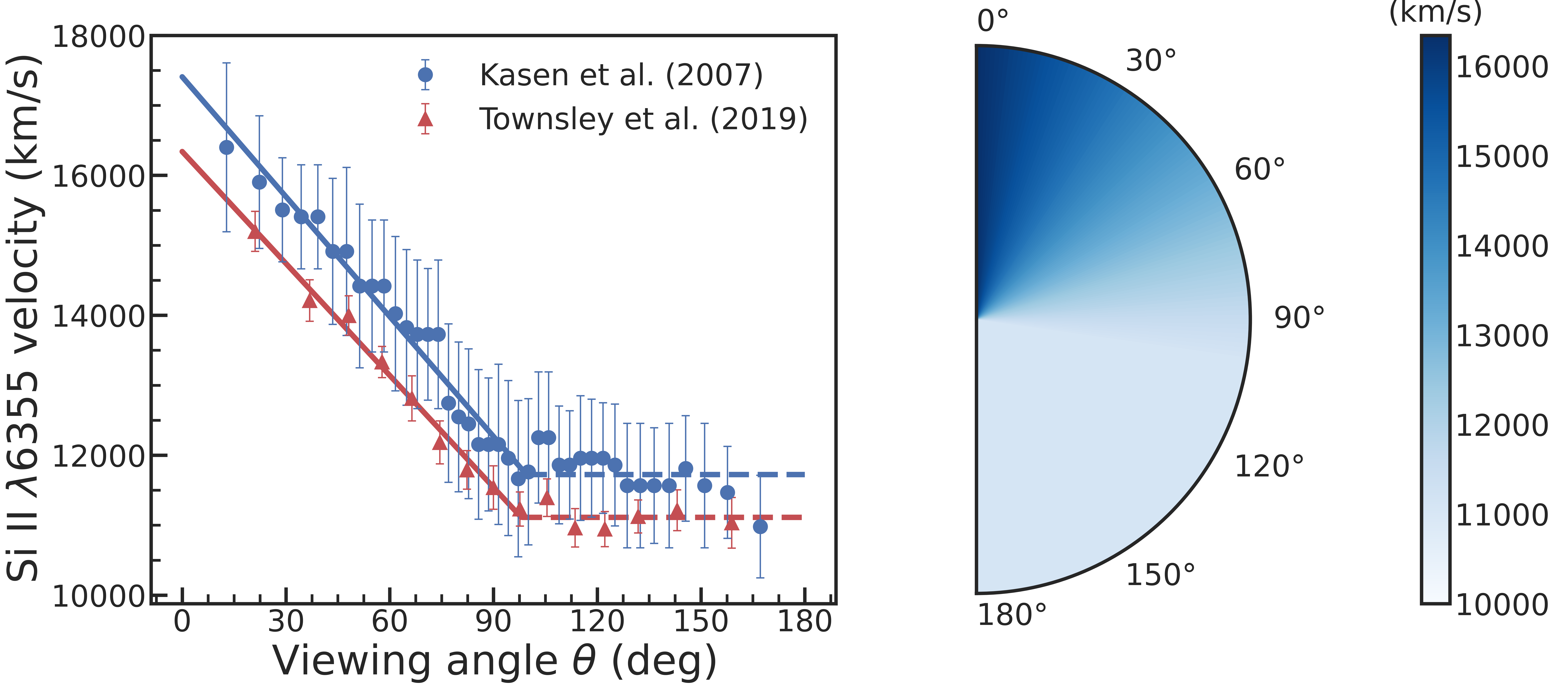
Townsley et al. 2019 considered a double detonation that ignites first in a helium shell on the surface of the white dwarf; the He shell is heated by a directly impacting accretion stream and mixes modestly with the outer edge of the core. They use a white dwarf with a $1.0\text{\,}\mathrm{M}_{\odot}$ C-O core and a surface He layer with base $\rho=$2\text{\times}{10}^{5}\text{\,}\mathrm{g}\text{\,}{\mathrm{cm}}^{-3}$$ and $T=$5\text{\times}{10}^{8}\text{\,}\mathrm{K}$$, having a mass of $0.021\text{\,}\mathrm{M}_{\odot}$. The He detonation is ignited with a spherical hotspot placed on the symmetry axis at the base of the He layer. Maximum-light spectra are synthesised at different averaged viewing angles (see 4 of Townsley et al. 2019). Again, we measure the Si II $\lambda$6355 velocity and plot the results in Figure 4, shown as red circles.

One can see that both models give very similar behavior for the Si II $\lambda$6355 velocity as a function of viewing angle: the highest velocity appears at $\theta=$$$. The velocity decreases linearly as the viewing angle increases (toward the detonation side). But after $\theta$ around $100°$, near the equator, the velocity becomes constant with almost no changes. To mathematically quantify this evolution, we use the following monotonically decreasing function to describe the data:

To simulate the distribution of velocities, we generate a sample size of $N=$10,000$$ SN Ia cutoff velocities $v_{c}$ individually sampled from the Group I Gaussian distribution, henceforth calling this sample the intrinsic distribution, which is also the input distribution for our simulation. We then consider the asymmetry effect according to the different parameters, applying it to a certain fraction of the SNe Ia (see details below); thus, the asymmetry-corrected velocity distribution, which is also the output sample from our simulation, changes from the intrinsic (input) distribution. We finally compare the asymmetry-corrected (output) velocity distribution with the observed distribution by adopting the KS test in order to find the best parameters. We define the parameter space from a grid search allowing the parameters to be within their respective ranges: $\theta_{c}\in\left\{$$,$$,$$,\ldots,$$\right\}$ with an increment of $1°$, and $\Delta v\in\left\{3000,3100,3200,\ldots,7500\right\}$\mathrm{km}\text{\,}{\mathrm{s}}^{-1}$$ with an increment of $100\text{\,}\mathrm{km}\text{\,}{\mathrm{s}}^{-1}$, giving a space of size 8280 pairs of parameters. The parameters are ranked by the KS values, and we select the top four best parameters for further discussion from the total of 8280 pairs of parameters. The simulation codes are written in Python 3 and can be found online. ³³ 3 https://github.com/ketozhang/ejecta_velocities_of_type_Ia_supernovae.

We consider two cases for the asymmetry effect in our simulation: (1) only a portion of the SNe Ia from the intrinsic distribution are asymmetric, and (2) all of the SNe Ia from the intrinsic distribution are asymmetric.

For Case 1, considering the mean and scatter parameters of the two groups, it is natural to assume that Group I SNe Ia are symmetric while Group II SNe Ia are asymmetric, and we therefore assume 35% of the intrinsic distribution (namely the total number of Group II SNe Ia) need to be corrected for asymmetry from the intrinsic (input) distribution. To do this, we first generate $N=10^{5}$ SN Ia velocities sampled from a Gaussian distribution with parameters taken from Group I SNe Ia ($\mu=$11,000\text{\,}\mathrm{km}\text{\,}{\mathrm{s}}^{-1}$$ and $\sigma=$700\text{\,}\mathrm{km}\text{\,}{\mathrm{s}}^{-1}$$). 64.6% of these SNe Ia (namely the total number in Group I) are unmodified and passed onto the final output result. For the remaining 35% of SNe Ia, being Group II, we treat them by applying the asymmetry model (Eq. 8), where $v_{c}$ is taken from the generated velocities of the intrinsic distribution (i.e., $v_{c}$ is sampled from the Group I Gaussian distribution), while $\theta_{c}$ and $\Delta_{v}$ are taken from the parameter space. The asymmetry-corrected (output) velocity for the final result is then calculated assuming the SN is equally observable in each unit solid angle. We achieve this by applying the spherical point-picking correction to the viewing angle $\theta=\arccos(2u-1)$, where $u$ samples the uniform$(0\,,1)$ distribution. We finally compare the asymmetry-corrected velocity distribution for all $10^{5}$ SNe Ia with the observed distribution of 311 SNe Ia by adopting the KS test. This step is repeated for a total of 8280 sets of parameters $\theta_{c}$ and $\Delta v$ in the parameter space.

Here we show the top four performing parameter sets in the KS test, as plotted in Figure 5. The KS statistic computes a distance between the empirical distribution of the simulation of $10^{5}$ SNe Ia and the observed sample of 311 SNe Ia. The $p$-value is two-tailed, generated from the KS statistic and the null hypothesis that the two distributions come from the same population distribution. For reference, the KS statistic with the naive hypothesis that the underlying distribution is Gaussian with Group I parameters tested with the observed data produces a KS value of $0.19$ and a $p$-value of $6.43\text{\times}{10}^{-10}$; hence, we strongly reject the hypothesis that the observed data are normally distributed with Group I parameters. For the top four performing results shown in Figure 5, with an $\alpha$ level of 5%, the null hypothesis cannot be rejected. The best parameters out of the top four cases are $\theta_{c}=$$$ and $\Delta v=$6000\text{\,}\mathrm{km}\text{\,}{\mathrm{s}}^{-1}$$ with a KS value of $3.2\text{\times}{10}^{-02}$ and a $p$-value of $0.91$. All four top cases have very similar best parameters, with $\theta_{c}$ in the range $110\text{\,}\mathrm{\SIUnitSymbolDegree}112\text{\,}\mathrm{\SIUnitSymbolDegree}$ and $\Delta v$ of $5900\text{\,}\mathrm{km}\text{\,}{\mathrm{s}}^{-1}6300\text{\,}\mathrm{km}\text{\,}{\mathrm{s}}^{-1}$. These parameters are very close to the values from the two asymmetric models given in Section 4.1. To produce confidence intervals, we create a joint probability space where the values are the parameters and the chance to observe the parameters is the $p$-value normalised by dividing the $p$-value with the sum of all 8280 $p$-values from the simulations. This probability space is then sampled $10,000$ times to get a parameter distribution where the mean and standard deviation are used for the $1\sigma$ confidence interval. Doing so, the $1\sigma$ confidence interval is $\theta_{c}=$120\pm 15\text{\,}\mathrm{\SIUnitSymbolDegree}$$ and $\Delta v=$5400\pm 1200\text{\,}\mathrm{km}\text{\,}{\mathrm{s}}^{-1}$$ at 1$\sigma$ confidence.

For Case 2, instead of applying the asymmetric model to a subset of the intrinsic (input) distribution, we apply the asymmetric model to all $N=$10,000$$ simulated SNe Ia from the intrinsic (input) distribution. Thus, we assume that all SNe Ia are asymmetric. The remaining simulation procedures follow exactly as in the Case 1. Similarly, we show the top four performing results in Figure 6. At an $\alpha$ level of 5%, the null hypothesis for all four top cases cannot be rejected, the same as in Case 1. The best parameters out of the top four simulations are $\theta_{c}=$$$ and $\Delta v=$6400\text{\,}\mathrm{km}\text{\,}{\mathrm{s}}^{-1}$$, with a KS value of $3.3\text{\times}{10}^{-02}$ and a $p$-value of $0.89$. The $1\sigma$ confidence interval is calculated to be $\theta_{c}=$63\pm 6\text{\,}\mathrm{\SIUnitSymbolDegree}$$ and $\Delta v=$5700\pm 1100\text{\,}\mathrm{km}\text{\,}{\mathrm{s}}^{-1}$$. Compared to Case 1, the obvious difference is in $\theta_{c}$: for Case 2, $\theta_{c}$ is around $63°$, which is much smaller than in Case 1 ($\theta_{c}\approx$$$). The other parameter, $\Delta v$, is almost the same as for Case 1.

For both cases, at an $\alpha$ level of 5%, the null hypothesis for all four top simulations cannot be rejected, which indicates that for both cases, the simulations can reproduce the observed Si II $\lambda$6355 velocity distribution. Also, while comparing to the models, both cases give a cutoff velocity $\Delta v$ around $5500\text{\,}\mathrm{km}\text{\,}{\mathrm{s}}^{-1}$, matching well to the two models ($5200\text{\,}\mathrm{km}\text{\,}{\mathrm{s}}^{-1}$ and $5700\text{\,}\mathrm{km}\text{\,}{\mathrm{s}}^{-1}$). However, for the other parameter, the cutoff angle $\theta_{c}$, Case 1 is apparently better than Case 2. The $\theta_{c}$ parameter from both models is $\phantom{}\sim 100°$. From Case 1, $\theta_{c}$ is $\phantom{}\sim 120°$, slightly larger, but much closer to $100°$ compared to Case 2, for which $\theta_{c}$ is $\phantom{}\sim 63°$. For this reason, we favor Case 1 over Case 2.

As shown above, our simulations indicate that assuming a portion of SNe Ia are asymmetric, we can reproduce the observed Si II $\lambda$6355 velocity distribution (Case 1). The asymmetric SNe Ia could occupy a notable fraction (35%) of the total SNe Ia. In fact, since the $\theta_{c}$ value in Case 1 $120\pm \pm 15°$ is slightly larger than in the model ($\phantom{}\sim 100°$), while increasing the fraction of asymmetric SNe Ia in the simulation would reduce the $\theta_{c}$ value, a larger fraction of asymmetric SNe Ia would provide a better match between the simulation $\theta_{c}$ and the model; therefore our simulation indicates that more than 35% of SNe Ia are asymmetric. Note that for both cases, since the input distribution is the same for all SNe, all SNe Ia share the same intrinsic velocity distribution in our simulation. Even for Case 1, where 35% are asymmetric, all SNe Ia still share the same input distribution. The only difference is that the output distribution for the 35% SNe Ia are asymmetry-corrected. We therefore conclude that more than 35% of SNe Ia are asymmetric from our simulation if all SNe Ia share the same intrinsic velocity distribution based on the adopted models and simulations.

References

- Akaike (1974) Akaike H., 1974, IEEE Transactions on Automatic Control, 19, 716
- Blondin et al. (2012) Blondin S., et al., 2012, AJ, 143, 126
- Bloom et al. (2012) Bloom J. S., et al., 2012, ApJ, 744, L17
- Cao et al. (2015) Cao Y., et al., 2015, Nature, 521, 328
- Cikota et al. (2019) Cikota A., et al., 2019, MNRAS, 490, 578
- Dong et al. (2015) Dong S., Katz B., Kushnir D., Prieto J. L., 2015, MNRAS, 454, L61
- Filippenko (1997) Filippenko A. V., 1997, ARA&A, 35, 309
- Folatelli et al. (2013) Folatelli G., Morrell N., Phillips M. M., et al., 2013, ApJ, 773, 53
- Foley & Kasen (2011) Foley R. J., Kasen D., 2011, ApJ, 729, 55
- Foley et al. (2011) Foley R. J., Sanders N. E., Kirshner R. P., 2011, ApJ, 742, 89
- Goobar et al. (2014) Goobar A., et al., 2014, ApJ, 784, L12
- Han et al. (2020) Han X., et al., 2020, ApJ, 892, 142
- Hillebrandt & Niemeyer (2000) Hillebrandt W., Niemeyer J. C., 2000, ARA&A, 38, 191
- Holmbo et al. (2019) Holmbo S., et al., 2019, A&A, 627, A174
- Horváth (1998) Horváth I., 1998, ApJ, 508, 757
- Horváth et al. (2008) Horváth I., Balázs L. G., Bagoly Z., Veres P., 2008, A&A, 489, L1
- Hosseinzadeh et al. (2017) Hosseinzadeh G., et al., 2017, ApJ, 845, L11
- Howell (2011) Howell D. A., 2011, Nature Communications, 2, 350
- Iben & Tutukov (1984) Iben Jr. I., Tutukov A. V., 1984, ApJS, 54, 335
- Im et al. (2015) Im M., Choi C., Yoon S.-C., Kim J.-W., Ehgamberdiev S. A., Monard L. A. G., Sung H.-I., 2015, ApJS, 221, 22
- Jha et al. (2019) Jha S. W., Maguire K., Sullivan M., 2019, Nature Astronomy, 3, 706
- Kasen (2010) Kasen D., 2010, ApJ, 708, 1025
- Kasen & Plewa (2007) Kasen D., Plewa T., 2007, ApJ, 662, 459
- Kasen & Woosley (2009) Kasen D., Woosley S. E., 2009, ApJ, 703, 2205
- Kass & Raftery (1995) Kass R. E., Raftery A. E., 1995, Journal of the American Statistical Association, 90, 773
- Kawabata et al. (2019) Kawabata M., et al., 2019, arXiv e-prints, p. arXiv:1908.03001
- Kushnir et al. (2013) Kushnir D., Katz B., Dong S., Livne E., Fernández R., 2013, ApJ, 778, L37
- Levanon & Soker (2019) Levanon N., Soker N., 2019, MNRAS, 486, 5528
- Li et al. (2019) Li W., et al., 2019, ApJ, 870, 12
- Maund et al. (2010) Maund J. R., et al., 2010, ApJ, 725, L167
- Moll et al. (2014) Moll R., Raskin C., Kasen D., Woosley S. E., 2014, ApJ, 785, 105
- Mukherjee et al. (1998) Mukherjee S., Feigelson E. D., Jogesh Babu G., Murtagh F., Fraley C., Raftery A., 1998, ApJ, 508, 314
- Nugent et al. (2011) Nugent P. E., et al., 2011, Nature, 480, 344
- Pakmor et al. (2010) Pakmor R., Kromer M., Röpke F. K., Sim S. A., Ruiter A. J., Hillebrandt W., 2010, Nature, 463, 61
- Pakmor et al. (2012) Pakmor R., Kromer M., Taubenberger S., Sim S. A., Röpke F. K., Hillebrandt W., 2012, ApJ, 747, L10
- Perlmutter et al. (1999) Perlmutter S., Aldering G., Goldhaber G., et al., 1999, ApJ, 517, 565
- Plewa (2007) Plewa T., 2007, ApJ, 657, 942
- Polin et al. (2019) Polin A., Nugent P., Kasen D., 2019, ApJ, 873, 84
- Raskin et al. (2014) Raskin C., Kasen D., Moll R., Schwab J., Woosley S., 2014, ApJ, 788, 75
- Riess (2019) Riess A. G., 2019, Nature Reviews Physics, 2, 10
- Riess et al. (1998) Riess A. G., Filippenko A. V., Challis P., et al., 1998, AJ, 116, 1009
- Seitenzahl et al. (2013) Seitenzahl I. R., et al., 2013, MNRAS, 429, 1156
- Shen et al. (2018) Shen K. J., et al., 2018, ApJ, 865, 15
- Siebert et al. (2019) Siebert M. R., et al., 2019, MNRAS, 486, 5785
- Silverman et al. (2012a) Silverman J. M., Foley R. J., Filippenko A. V., et al., 2012a, MNRAS, 425, 1789
- Silverman et al. (2012b) Silverman J. M., Kong J. J., Filippenko A. V., 2012b, MNRAS, 425, 1819
- Silverman et al. (2012c) Silverman J. M., et al., 2012c, ApJ, 756, L7
- Sim et al. (2013) Sim S. A., et al., 2013, MNRAS, 436, 333
- Stahl et al. (2020) Stahl B. E., et al., 2020, MNRAS, 492, 4325
- Sugiura (1978) Sugiura N., 1978, Communications in Statistics - Theory and Methods, 7, 13
- Townsley et al. (2019) Townsley D. M., Miles B. J., Shen K. J., Kasen D., 2019, ApJ, 878, L38
- Wang & Wheeler (2008) Wang L., Wheeler J. C., 2008, ARA&A, 46, 433
- Wang et al. (2009) Wang X., et al., 2009, ApJ, 699, L139
- Wang et al. (2013) Wang X., Wang L., Filippenko A. V., Zhang T., Zhao X., 2013, Science, 340, 170
- Wang et al. (2019) Wang X., Chen J., Wang L., Hu M., Xi G., Yang Y., Zhao X., Li W., 2019, ApJ, 882, 120
- Webbink (1984) Webbink R. F., 1984, ApJ, 277, 355
- Whelan & Iben (1973) Whelan J., Iben Jr. I., 1973, ApJ, 186, 1007
- Zheng et al. (2013) Zheng W., et al., 2013, ApJ, 778, L15
- Zheng et al. (2017) Zheng W., et al., 2017, ApJ, 841, 64
- Zheng et al. (2018) Zheng W., Kelly P. L., Filippenko A. V., 2018, ApJ, 858, 104