Existence of solutions for deterministic bilevel games under a general Bayesian approach
Abstract
In 1996, Mallozzi and Morgan [33] proposed a new model for Stackelberg games which we refer here to as the Bayesian approach. The leader has only partial information about how followers select their reaction among possibly multiple optimal ones. This partial information is modeled as a decision-dependent distribution, the so-called belief of the leader. In this work, we formalize the setting of this approach for bilevel games admitting multiple leaders and we provide new results of existence of solutions. We pay particular attention to the fundamental case of linear bilevel problems, which has not been studied before, and which main difficulty is given by possible variations in the dimension of the reaction set of the follower. Our main technique to address this difficulty is based on a stronger notion of continuity for set-valued maps that we call rectangular continuity, and which is verified by the solution set of parametric linear problems. Finally, we provide some numerical experiments to address linear bilevel problems under the Bayesian approach.
Keywords Bilevel game, Bayesian approach, Belief, decision-dependent distribution, rectangular continuity, Differential Evolution.
Mathematics Subject Classification (2020) Primary: 91A65; Secondary: 90C15, 49J53
1 Introduction
The term bilevel games is here used to refer to non-cooperative models ranging from bilevel programming problems [15] to multi-leader-follower games [6, 26]. They were first introduced by H. von Stackelberg [48] in the 30’s to model hierarchical decision problems, and since the last few decades they have attracted the attention of many researchers, due to their large potential in applications. Bilevel games consist in a non-cooperative interaction between two or more agents, which are divided in two groups: the leaders and the followers. The main difference between these two groups of agents is that, on the one hand, leaders know how followers make their decisions, and so they are able to include this information in their own decision-making processes. On the other hand, followers are only capable of observing the decisions of the leaders once they have been made, and then react accordingly.
It is well known that, unless the followers’ reactions are unique, the problems of the leaders are ill-defined. To solve this issue, the most common approaches that we find in the literature are the Optimistic approach and the Pessimistic approach [15, 32]. A leader is optimistic, if he or she assumes that the followers will provide the reaction, among the optimal ones, that favors him or her the most. A leader is pessimistic, if he or she assumes that the followers will provide the reaction that harms him or her the most.
In many applied situations, however, followers are neither adversarial nor cooperative. Thus, some other approaches have been proposed as alternatives between the optimistic/pessimistic dichotomy, like using selections as single-valued reaction of the follower (see, e.g., [16, pp. 6]), or moderate approaches that consider convex combinations between the min/max values over the followers’ variables [2, 28].
We will focus our attention in a more general approach that was first introduced by L. Mallozzi and J. Morgan in [33] for bilevel games with one leader and which we refer here to as the Bayesian approach (see Remark 2). The approach works as follows: Each leader is endowed with a private belief about how followers select their reaction. This belief is modeled as a probability distribution over the set of optimal reactions. Then, leaders play a non-cooperative game, where each leader’s payoff function depends on his or her decision, the decisions of the other leaders, and his or her private belief.
Clearly, the Bayesian approach encloses both Optimistic and Pessimistic approaches, since optimism and pessimism can be modeled as beliefs. However, the price to pay is that beliefs are complex objects to work with, as they are decision-dependent distributions [29]. Programming with decision-dependent uncertainty has been explored recently in several works [1, 43, 40, 24, 19], and it is an active field of research due to its challenging difficulties, both from the theoretical and algorithmic point of view.
Literature review
In [33], the analysis of the Bayesian approach for bilevel games (with a single leader) is focused on the existence of solutions in two cases: first, when the reactions of the follower are finite, and second, when the values of the reaction map have positive Lebesgue measure (which is equivalent to have nonempty interior if they are convex). The second case has been applied to the so-called regularized bilevel problem, where the reaction map consists of approximate solutions of the lower-level problem being a convex parametric optimization problem. In [34], the above results have been adapted to reaction maps whose values have either nonempty interior or consist of a single point.
However, none of the results of [33, 34] can be applied to bilevel problems with reaction maps of varying affine dimension. In particular, they cannot be applied (in general) to linear bilevel problems with exact solutions on the lower-level.
To the best of our knowledge, there is no other contribution in the literature about the Bayesian approach, beyond the aforementioned works. This is somehow confirmed by the recent survey [13].
Our contributions
We first formalize a natural extension of the Bayesian approach to bilevel games, admitting multiple leaders. This is done in the Preliminaries (Section 2). In Section 3.1, we provide a general sufficient (and necessary, in some sense) condition to have existence of solutions for the Bayesian approach, which is the weak continuity of the beliefs in the sense of measure-valued maps. Weak continuity allows us to guarantee existence of solutions for the case of one leader (Theorem 2), and existence of mixed equilibria for the case of multiple leaders (Theorem 3).
In Section 3.2, we introduce a new notion of continuity, called rectangular continuity. Intuitively, a rectangularly continuous set-valued map might change the affine dimension of its values, but in a controlled fashion. We show, in Section 3.3, that if the reaction map of the followers in a bilevel game has convex values and it is rectangularly continuous, then all the beliefs coming from a continuous strictly positive density are weak continuous. This is our first main result, enclosed in Theorem 5.
Finally, in Section 3.4, we show that the solution maps of parametric linear problems of the form are not only continuous (which is well known), but they are rectangularly continuous. In fact, we prove this result for separable parametric problems given by weakly analytic functions in Theorem 6, for which parametric linear problems are a particular case. This is our second main contribution. Our results are new even in the case of linear bilevel programming, and this is summarized in Corollary 2.
In Section 4, we provide some numerical experiments for bilevel programming under the Neutral approach, which is the Bayesian approach with the belief induced by uniform distributions. For this numerical tests, we implement the differential evolution metaheuristic [12] and compute the Bayesian objective function through a Monte-Carlo method. We use the BOLIB library [52] as benchmark problems.
2 Preliminaries and model formulation
Throughout this article, we gather three main fields of mathematics that we assume the reader is acquainted with in a basic level: (Bilevel) Game theory [22, 47, 15], Set-valued analysis [3, 46] and Measure theory [30].
2.1 Notation
We will work on finite-dimensional spaces, namely , endowed with the Euclidean norm and the inner product . An open ball of radius and centered at is denoted by , and we write if the ball is centered at the origin. The closed unit ball centered at the origin will be denoted by . Given a subset of , we denote by , , , and , its closure, interior, boundary, relative interior and affine hull, respectively. The affine dimension of , that is, the dimension of , is denoted by . We denote by and the convex hull and the closed convex hull of , respectively. The orthogonal set to is the set
Given sets and we write and to denote the Minkowski addition and scalar multiplication, respectively.
For two points , we write to denote the closed segment enclosed by and . Similarly, we write , and , for the open segment, and the semi-open segments, respectively. For a nonempty closed convex set and a point , we denote by or by the metric projection of onto . If is a convex closed product set on the product space , we also denote by the parallel projection onto , by identifying with .
Given two nonempty sets and , and a set-valued map , we denote the (effective) domain of by , and the range of by . The graph of is denoted by .
Let be a nonempty closed set. We denote by the Borel -algebra of , that is, the -algebra generated by the topology in . We recall that a measure defined over is called a Borel measure. Given an integer , we will denote by the -dimensional Hausdorff measure. It is well-known that for every affine subspace of of dimension , coincides with the usual Lebesgue measure on (see, e.g., [20]). From now on, we will simply refer to as the -dimensional Lebesgue measure. In the full dimensional case () we omit the subindex, simply writing .
The centroid (also known as the barycenter) of a nonempty bounded convex set is given by
| (2.1) |
where . Observe that, since is strictly positive for convex sets, the centroid is always well-defined.
We denote by the family of all (Borel) probability measures on , endowed with the topology of weak convergence. Recall that a sequence weak converges to , which is denoted by , if
for all continuous functions with bounded support. It is well known that is metrizable for the induced topology by the weak convergence and, whenever is compact, then is compact as well (see, e.g., [30, Chapter 13]). Accordingly, we will say that a measure-valued map is weak continuous if for every sequence converging to a point , the sequence weak converges to .
Now, let us recall a sequence of equivalences for the weak convergence on , known as the Portemanteau Theorem (see, e.g., [30, Thm. 13.16], and [11, Excercise 2.6]).
Theorem 1 (Portemanteau).
Let be a nonempty closed subset of , be a sequence of probability measures of and let . The following assertions are equivalent:
- 1.
.
- 2.
, for every lower semicontinuous function bounded from below.
- 3.
, for every closed set in .
- 4.
, for every open set in .
2.2 Bilevel games and the Bayesian approach
Formally, a bilevel game is posed as follows. In the upper level, there is a finite set of players, usually known as the leaders, interacting in a non-cooperative Generalized Nash Equilibrium Problem (GNEP for short, see, e.g., [21]). A GNEP, is an equilibrium problem where the feasible strategies of each player might depend on the strategies of the other players. Thus, each leader has a decision variable and a function that he or she wishes to minimize, where we use the usual notation , to denote the other players’ strategy.
Given a leaders’ decision vector , the lower-level is represented by a set-valued map and a decision variable . This decision variable is chosen by a finite set of independent agents, called the followers, who react to the leaders’ decision vector . The set represents the solution set (or approximate solution set) of the followers’ problem which can be given by a parametric optimization problem [8], a parametric game [5], a parametric variational inequality [35], etc.
We will call the reaction map, and it will play a central role in our analysis. We refer to as the ambient space, and if it is not explicitly defined, one simply takes . In general, we will assume to be compact. Finally, each leader aims to solve the following problem:
| (2.2) |
In what follows, unless stated otherwise, we will always assume for each that is continuous, is nonempty and compact and that the set-valued map has closed graph. We will also assume that has closed graph, which in particular implies that has closed values (and hence also measurable).
Note that for some point , one might have that . In such a case, for each we consider the decision to be infeasible for problem , even if . Under the conventional abuse of notation that , we can always replace by for every and every . Therefore we will always assume that
| (2.3) |
This assumption, however, yields that a bilevel game has an intrinsic GNEP nature due to the possible empty values of , even if originally we considered for each and for each . This motivates the following distinction:
Definition 1 (Plain bilevel games).
We say that a bilevel game given by problems (2.2) is plain if for each and for each , and .
Observe that if the bilevel game is plain, then the leaders interact in a Nash equilibrium problem rather than in a GNEP.
If only one leader is involved, we omit the subindex , by considering the problem . In this setting, if is the solution set of a parametric optimization problem, the bilevel game is known as a bilevel programming problem (see, e.g., [15]). The general form of a bilevel programming problem is given by
| (2.4) |
where is the constraints set-valued map of the follower, usually of the form , where is a continuous vector-valued function and is continuous. The reaction map is then given by . Observe that in this case, assuming that the ambient space is compact, one has by Weierstrass Theorem that , that is, is nonempty whenever the lower-level problem is feasible. Thus, in this case, by replacing by , we can always assume that the lower-level is feasible within the feasible set . In other words, a bilevel game with only one leader can always be assumed to be plain.
Remark 1.
As explained in the introduction, the reaction map might not be single-valued at every point, so the bilevel problem carries an ambiguity that must be handled. In the literature the most common approaches are the Optimistic and Pessimistic ones (see, e.g., [32, 15]). In the rest of this section, we recall the Bayesian approach, which solves the ambiguity in a more general form by considering beliefs for the leaders. We start by providing a formal definition of what a belief over a set-valued map is.
Definition 2 (Belief).
Let be a nonempty subset of , be a nonempty closed subset of , and be a set-valued map with nonempty measurable values (i.e. for all ). A belief over is a mapping assigning to each a probability measure on such that
| (2.5) |
A finite collection of beliefs is called a belief system over .
In the case of a general bilevel game (2.2), we consider (or , according to (2.3)). For a plain bilevel game (such as the case with a single leader), we set .
If a leader has a belief over , it means that for a given leaders’ decision vector , he or she predicts that the reaction of the followers is a random variable with probability distribution . Accordingly, he or she aims to minimize the expected value of his/her cost function , with respect to . Thus, problem (2.2) can be formulated as follows:
| (2.6) |
Note that, since the belief is fixed (in the sense that it is not decided within problem (2.6) but prior to it), the equilibrium problem given by (2.6) becomes a generalized Nash equilibrium problem (GNEP), where all the complexity of the bilevel structure is captured by the beliefs. In this GNEP the objectives of the players are no longer random, and we will call it a bilevel game with belief system .
The Bayesian approach consists in selecting a belief system, prior to the problem, that models the predictions of the leaders to the uncertain followers’ reactions, and then to pose the problem as the bilevel game with the selected belief system.
Remark 2.
The renaming of the approach as Bayesian is motivated by several aspects: First, it encompasses the fact that leaders must form beliefs over the (unknown) behavior of the followers which fits the Bayesian interpretation of probabilities (see, e.g., [49]). Secondly, these beliefs can be understood as priors, that could be refined after playing the game. While this is not treated in this work, the idea opens the possibility of “learning” the real behavior of the followers by updating the belief and observing outcomes of the game. Finally, considering that the selection is unknown due to lack of information, one might understand it as the type of the follower, following the ideas of Bayesian games [25].
2.3 Scope of the work
The present work is about existence of solutions of Problem (2.6). The scope of this article is highlighted by the following assumptions.
(A) We will consider only plain bilevel games
If the bilevel game is not plain, Problem (2.6) is a GNEP. Positive results for existence of equilibria for GNEPs are very few and they rely on either some generalized convexity condition or ideas coming from potential games. These conditions are generally not reasonable for bilevel games. Furthermore, up to the best of our knowledge, there is no good notion of mixed equilibrium for GNEP. Thus, we will restrain ourselves to the setting where Problem (2.6) is a NEP, which are plain bilevel games (including general single-leader games).
(B) We will assume that takes convex values
While this is a simplifying assumption, the cases where takes convex values encompasses several important settings such as the case where is the solution of a parametric convex programming problem, or the case where is the set of correlated equilibria of a Nash game with finite strategy sets (see, e.g., [42]). In particular, this is the setting of bilevel games where the lower-level is given by a parametric linear problem of the form , which is our main motivation.
(C) We will assume that the beliefs are nonatomic
Our main results are focused on beliefs that are absolutely continuous with respect to the (corresponding) Lebesgue measures. Specifically, we mean that for every and every ,
where and is the Lebesgue measure over .
An important belief that we shall consider in this setting (and that will lead our efforts in the following sections) is the one given by uniform distributions over the sets . This belief models the situation where the leader has no information over how the followers select their reaction, hence assigning equal density to each possible one.
Definition 3 (Neutral belief).
Let be a nonempty closed subset of and let be a set-valued map with nonempty convex compact values. The Neutral belief over is given by
where and is the -dimensional Lebesgue measure.
The Neutral approach is then given as the equilibrium problem (2.6) where each leader minimizes the value function
| (2.7) |
3 Existence of solutions for the Bayesian approach
This section is devoted to study the existence of solutions for the Bayesian approach, based on sufficient conditions related to the reaction map and the belief over .
3.1 Existence results for weak continuous beliefs
Here we will show two existence results for the problem defined by (2.6) under the hypothesis that the belief of each leader is weak continuous.
Theorem 2.
Let be a nonempty compact set of and let us consider a bilevel game given by (2.6) with only one leader (i.e., ) with belief over . If one has that
- (i)
the cost function is lower semicontinuous,
- (ii)
the constraints set is nonempty and compact, and
- (iii)
the belief is weak continuous,
then, is lower semicontinuous and so, the (single leader) bilevel game admits at least one solution in the Bayesian approach.
Proof.
We will only show the lower semicontinuity of since the existence of solutions will trivially follow from the compactness of . Let be a sequence converging to a point .
Fix . Since is lower semicontinuous, for each there exists a neighborhood of such that and
Without loss of generality, we may choose to be closed. Now, since is compact, there exists a finite cover of , included in . Let be a finite sequence such that . Consider the neighborhood of given by . Note that satisfies
for each . Let us define the function given by
By construction, is lower semicontinuous, bounded from below and satisfies for any . In particular, for large enough , and hence, for every , we have . This yields, by the Portemanteau Theorem (see Theorem 1), that
Now, let and let . We claim that converges pointwise to . Indeed, choose . First, since for every , it is clear that .
By construction, for each , there exists such that
Then, we can write
where the last inequality follows from the fact that is lower semicontinuous and that . Thus, we have shown that
proving that . and, by arbitrariness of , proving our claim.
Now, since attains its minimum over , we have that for every , , and so, applying the Fatou Lemma for the measure , we can write that
Since was an arbitrary sequence, we have shown the lower semicontinuity of the mapping , which finishes the proof. ∎
Remark 3.
The weak continuity of the belief is used as a sufficient condition in Theorem 2 to prove the lower semicontinuity of the Bayesian objective function of the leader given by
Conversely, if we require that the Bayesian objective function of the leader to be lower semicontinuous for any lower semicontinuous objective function , then the belief must be weak continuous. This follows directly from part 2 of the Portemanteau Theorem by considering a lower semicontinuous function and the leader’s objective . In this sense, weak continuity of the belief is also necessary.
When multiple players are involved, the Bayesian approach suffers the same drawback as the rest of the approaches: it is a nonconvex generalized Nash equilibrium problem. While sufficient conditions to have existence of equilibria have been provided in the literature as generalized convexity conditions (see e.g. [14, 10]), these are generally not satisfied in the context of bilevel games (see [41, Example 4]). Nevertheless, leaders can randomize their decisions in the setting of plain bilevel games. Then we can derive existence of mixed equilibria (introduced by Nash [39] in the case of finite strategy sets, and extended to compact strategy sets one year later by Glicksberg [23]). In the next definition, we recall the notion of Mixed Equilibrium for compact strategy sets.
Definition 4 (Mixed equilibrium).
Let us consider a Nash Equilibrium problem with players, where each player aims to solve
and all the objective functions are measurable and bounded from below. A mixed strategy of player is a probability measure . An -tuple in is called a mixed equilibrium, if for each player ,
where stands for the product measure on .
The concept of mixed equilibria has been explored for bilevel games with continuous strategy sets in the setting of electricity auctions in [44]. Recent efforts have been made to provide methods to compute them for Nash equilibrium problems with continuous strategy sets [18], but it is still a challenging research problem.
By considering the objective functions , we can derive the following direct theorem of existence of mixed equilibria for the Bayesian approach. The proof is similar to Theorem 2, and the conclusion follows by applying Glicksberg Theorem [23].
Theorem 3.
Let be a nonempty compact set of and let us consider the bilevel game given by (2.2). Assume that this is a plain bilevel game, and consider the Bayesian approach (2.6) with belief system over . If for each leader one has that
- (i)
the cost function is continuous,
- (ii)
the global decision set is nonempty and compact,
- (iii)
the belief is weak continuous,
then, is continuous for each , and so the bilevel game in the Bayesian approach admits a mixed equilibrium.
Proof.
Assuming that the bilevel game is plain, Problem (2.6) can be rewritten as
| (3.1) |
Here, each belief is well-defined due to the fact that in plain bilevel games we have that . Now, using the same argument as in the proof of Theorem 2 we can show that for each both and are both lower semicontinuous. Thus is continuous and we conclude thanks to the Glicksberg Theorem [23]. ∎
Note that in general, any selection constitutes a belief (for plain bilevel games; otherwise we replace by ), and no other condition is needed to define Problem (2.6). However, both existence results require the involved beliefs to be weak continuous. This is a strong property for a belief and, in particular, it entails that must be a Markov kernel (see, e.g., [30, Definition 8.25]) in the sense that
- •
For each , is a Borel probability measure over ; and
- •
For each , is a -measurable map.
The first condition is trivially verified by definition, and the second one follows as a consequence of weak continuity: Indeed, it is enough to consider the maps with an open subset of (which is a -system of ), and deduce from Theorem 1 that the mappings are lower semicontinuous, and therefore measurable (then, the desired conclusion follows from, e.g., [30, Remark 2.6]). While being a Markov kernel ensures several nice properties for a belief such as the measurability of and the well-posedness of mixed strategies (see Definition 4), it is not enough to guarantee existence of solutions for the Bayesian approach, as the following (classic) example shows.
Example 1.
Consider and given by
Then, any belief over must have the form
for some probability measure , where stands for the delta measure at point . In this case, all beliefs are Markov kernels, but none of them are weak continuous.
Remark 4.
It is worth to note that the probability distributions obtained in a mixed strategy describe how leaders randomize their decision process. Following the two-stage interpretation of bilevel games, they describe how the random decision vector is produced in a first stage. In contrast, the beliefs model how the reaction might be produced in a second stage, as a function of a decision that has been already produced.
3.2 Rectangular continuity of set-valued maps
Most common probability distributions used in applications are derived from the uniform distribution (through a continuous density with respect to the Lebesgue measure). In our context, this core distribution is given by the Neutral belief (recall Definition 3). Thus, we want to find sufficient conditions on the reaction map , such that at least the Neutral belief is weak continuous. We will motivate the conditions with a simple example that shows usual continuity is not enough, by analyzing the centroid of the map. In fact, the conditions should guarantee that the centroid mapping is continuous, as the next lemma shows.
Lemma 1.
Let be a nonempty closed subset of , and be a continuous set-valued map with nonempty convex compact values. If the Neutral belief over is weak continuous, then the centroid map is continuous.
Proof.
Fix . By definition, the centroid of is given by the vector integral
where is the th canonical vector of . Since for each the functional is continuous, then by Theorem 1 the weak continuity of yields that the mapping is continuous. ∎
A first guess of sufficient conditions for the weak continuity of the Neutral belief could be that the reaction map is continuous with convex values. However, in view of Lemma 1, the following example reveals that it is not so.
Example 2.
Let us consider the set-valued map defined by
which is clearly continuous and convex valued. We will call this map the triangle-to-segment map. Clearly, the centroid of is for , while the centroid of is . We see thus that the centroid mapping is not continuous at . In contrast, consider the map defined by
which we call the rectangle-to-segment map. Clearly, satisfies that its centroid, given by , is continuous. See Figure 3.1.
The main problem with the triangle-to-segment map in the above example is that for all , the set is not “balanced”, concentrating half of the “mass” of the triangle in the third right part of it. In contrast, the limit set is balanced in the sense that its “mass” is equally distributed in both halves. Continuity of is not enough to prevent this abrupt change in “mass” distribution. Motivated by the rectangle-to-segment map , we introduce a stronger notion of continuity of set-valued maps, that ensures that changes of dimension may happen but in a “balanced way”. As we will see in Section 3.3, this notion is sufficient to ensure weak continuity not only for the Neutral belief, but also for a large family of beliefs built from continuous densities. The idea is to use an inner and an outer approximation of by “rectangles” whose volume ratio goes to 1.
Definition 5.
(Rectangular continuity) Let nonempty and nonempty and closed. Let be a set-valued map with nonempty, bounded values. Let for each , and let . We say that is rectangularly continuous at if there exist maps such that
- 1.
For every near ,
(3.2) - 2.
For , , and has constant affine dimension equal to .
- 3.
For ,
(3.3) - 4.
The maps and have measurable values and verify that
(3.4)
We say that is rectangularly continuous on if it is so at each point .
We propose the name of rectangular continuity since the inclusions in (3.2) enclose between a rectangular-sum of sets: the “horizontal parts” and converge to , while the “vertical parts” and converge to , but keeping the same proportion as stated by equation (3.4). In the above definition, equation (3.4) is equivalent to
Rectangular continuity at implies continuity at . This follows directly from (3.3) and the Sandwich inclusion in (3.2). The reciprocal implication is not always true (Example 2 fails to verify rectangular continuity at ). The following proposition provides some direct cases where rectangular continuity is verified.
Proposition 1.
Let be a nonempty compact subset of , and let be a set-valued map with nonempty closed values, that is continuous at . Assume that one of the following conditions hold:
- 1.
is a singleton.
- 2.
is of constant affine dimension near .
- 3.
is convex-valued and has nonempty interior.
- 4.
is convex-valued with , that is, if .
Then, is rectangularly continuous at .
Proof.
The first assertion is verified by taking, for , as a single-valued selection of and . The second one comes from taking and , for . The third one is a consequence of the second one, since in this case has full affine dimension for all near . The fourth case is a consequence of the first and the third cases, since when , the lower semicontinuity of yields either that is a singleton, or that has full affine dimension near . ∎
It is important to observe that rectangular continuity really goes beyond the cases described in Proposition 1 as we shall see in Section 3.4. The following example provides a nontrivial set-valued map which is rectangularly continuous precisely because the changes of affine dimension can be “controled” by rectangular decomposition.
Example 3.
Let us consider the set-valued map given by
Clearly where is the support of . Thus, the affine dimension of ranges from to having points where for any integer in between. Figure 3.2 illustrates when .
3.3 Construction of weak continuous beliefs through densities
This section is devoted to show that rectangular continuity is sufficient to ensure weak continuity of certain beliefs that have a “density” with respect to Lebesgue measures in the corresponding affine subspaces.
Definition 6 (Beliefs with density function).
Let be a nonempty closed subset of and be a set-valued map with nonempty closed values. A belief over is said to admit a density function with respect to the neutral belief (or simply to admit a density), if there exists a function such that
- 1.
For all , restricted to is -measurable with
- 2.
And, for all
(3.5)
where . In such a case, we call a density function of .
The name density function is inspired in Markov kernels with densities (see, e.g., [7, Definition 1.2.4]), which are kernels where each measure can be written as
for some fixed measure . However, our definition is a little different, since the density function is integrated with respect to the Lebesgue measure associated to the moving set , instead of the (fixed) Lebesgue measure of . Note that the density function of a belief is not uniquely defined. However, if a belief admits a density function , then
| (3.6) |
where is the Radon-Nikodym derivative of with respect to , over the measurable space . It is worth noting that one could consider densities with respect to other beliefs, just by replacing the role of the Neutral belief in Definition 6.
We start our development with the following lemma that links the continuity of a set-valued map with the continuity of a measure evaluated in the images of .
Lemma 2.
Let be a nonempty closed subset of and let be a finite Borel measure on . Let be a set-valued map with measurable values and let . The following assertions hold:
- 1.
If is upper semicontinuous at , then is upper semicontinuous at .
- 2.
If is lower semicontinuous at , with compact convex values near , and , then is lower semicontinuous at .
Proof.
1. Consider the sequence of sets decreases to , that is, for all and . Then, by continuity of the measure, there exists such that . Now since is upper semicontinuous, there exists such that for any , and so . Putting both inequalities together, we have
Since the above argument works for any , we have proved that is upper semicontinuous at .
2. If , then . Thus, the lower semicontinuity of at follows trivially from the non-negativity of . Assume then that is nonempty and let us consider the sequence of sets defined by
Clearly, increases to , that is, and for all . Thus, by the continuity of the measure, given there exists such that
| (3.7) |
where the first equality is due to the assumption . Now, from the lower semicontinuity of at (see [46, Proposition 5.12]) we know there exists such that
Since , we get that for any one has
Using the cancellation law for convex sets (see [46, Corollary 3.35]), we obtain that for every , and so . Combining this last inequality with (3.7) we get
which proves the lower semicontinuity of at . ∎
For a solution map whose values are full-dimensional, we can state a first theorem that provides sufficient conditions to ensure weak continuity of beliefs admitting density functions, in the spirit of [33, Theorem 3.1]. Here, we write , as the usual space of Lebesgue-integrable functions over , with .
Theorem 4.
Let be a nonempty convex compact subset of , be a set-valued map with nonempty convex and compact values, and . Suppose that is continuous at and that the relative interior of with respect to is nonempty, for each near . Let be a belief over with a density function that satisfies that is -continuous at , that is,
Then, is weak continuous at .
Proof.
Without losing any generality, we assume that has nonempty interior. Define the measure given by
By Lemma 2, the mapping is continuous at and, for any closed subset intersecting , the mapping is upper semicontinuous at . Let be a closed subset of . By the Portemanteau Theorem, it is enough to prove that
Such inequality holds trivially if , due to the upper semicontinuity of . Thus, we assume that . Now, for near enough to we have that is strictly positive, and so we can write
The proof is then finished. ∎
By invoking Theorem 2, the above result yields the following direct corollary, that recovers the existence result of [33, Theorem 3.2] for regularized bilevel programs with continuous data.
Corollary 1.
Let be a nonempty convex compact subset of . Let us consider a bilevel game given by (2.6) with only one leader (i.e., ), for which is given as the -argmin of a lower-level problem for some fixed , that is,
| (3.8) |
If and are continuous and is nonempty compact, then the Bayesian approach admits a solution for any belief over with a density function satisfying that is -continuous.
To continue, we study set-valued maps with constant affine dimension, but not necessarily full-dimensional. This condition is a particular case of rectangular continuity, as stated in Proposition 1.
Lemma 3.
Let be a nonempty closed subset of and let . Let be a set-valued map with nonempty convex and compact values, and with constant affine dimension , which is continuous at . For any continuous function , the decision-dependent measure given by
satisfies that the mapping is continuous at .
Proof.
We divide the proof in two steps: First we will show the result for , that is, for ; and secondly for the general case.
Step 1: Define , where and . The map is clearly nonempty and convex valued and moreover, must be continuous at .
To prove the continuity of at , we will first show that is continuous at . To do so, we will construct single-valued mappings with such that all are continuous at and that is an orthogonal unit basis of for each near enough to .
Since is lower semicontinuous at , it is easy to verify that there exists a selection of which is continuous at . Replacing by , we may and do assume that for each , and thus . Clearly, for each .
Now, let be a basis of . For each , we can define the set-valued map given by
It is not hard to verify that for each , remains lower semicontinuous at , and so we know that there exists a selection of which is continuous at . Clearly, the mappings are also selections of and, by construction, is linearly independent. It is known that (see, e.g., [45, Chapter 5, Exercise 43a]) the continuity of the selections at ensures that there is a neighborhood of such that
| (3.9) |
Without losing generality, let us assume that . Now, applying the classic Gram-Schmidt algorithm, we can define the mappings for each where is an orthogonal unit basis of . It is not hard to see that the mappings remain continuous at , and so the desired construction is then completed.
Now, to prove that is continuous at , it is enough to show that
For the first inclusion, choose a sequence converging to and a sequence converging to , satisfying that for each . We need to show that .
Firstly, since for each , it is clear that . Now, on the one hand, since , we have that . On the other hand, for , we can write
which yields, by continuity at of the mappings , that
We deduce that , proving that and so .
Now, for the second inclusion, choose a a sequence converging to and a point . We need to show that there exists a sequence converging to and satisfying that for all large enough.
Consider then, the sequence defined by . Since , we get that for each . Furthermore, by construction and so for each . As we did before,
The proof is finished by noting that, since , then . We have shown then that the set-valued map is continuous at . Now, is the sum of two set-valued maps that are continuous at , one of them being locally bounded, then is also continuous at (see e.g. Exercise 5.24 in [46]). To finish Step 1, we observe that
where (Lemma 2) and is a positive constant. Form this it directly follows that is continuous at .
Step 2: Let be any sequence converging to . We need to show that
By upper semicontinuity of , we can assume that . Fix . Let be a open neighborhood of in such that . Such a neighborhood exists by continuity of (see, e.g. [27, Theorem 2.3.1]). By shrinking if necessary, there exists a finite measurable partition of such that for all . Then, for large enough (such that ) and for every , we can write
By summing the above inequalities through , we get that
Using a similar argument, we can show that
where the convergence follows from Step 1 of this proof. Since is arbitrary, the proof is finished. ∎
Now, we are ready to state and prove the main result of this section.
Theorem 5.
Let be a nonempty compact subset of , be a set-valued map with nonempty convex values, and let . Let be a belief over with continuous density function . If is rectangularly continuous at , then is weak continuous at . In particular, the Neutral belief over is weak continuous under rectangular continuity of .
Proof.
Let us consider an arbitrary sequence . The theorem is reduced to prove that
We divide the proof of this into two steps: In Step 1 we consider the case when has constant affine dimension, while in Step 2 we consider the general case of a rectangularly continuous . In the latter case, from the definition of rectangular continuity, is enclosed between and , where and have both constant affine dimension. Thus, we exploit what was proved in Step 1.
Step 1: Let us assume here that has constant affine dimension for all . From the Portemanteau Theorem (see Theorem 1) it is enough to prove that for any closed set we have
| (3.10) |
Define the set-valued map given by , where . If , then the upper semicontinuity of at will entail that near , and inequality (3.10) would follow trivially. Thus, let us assume that . Using the same arguments as in the first step of the proof of Lemma 3, we know that is upper semicontinuous. Thus, by Lemma 2,
which entails that is upper semicontinuous at . Then, we can easily adapt the same development of the second step of the proof of Lemma 3, to conclude that
Finally, using Lemma 3, we can write
The proof of the first part is finished.
Step 2: Now, we consider the general case. From the Portemanteau Theorem (see Theorem 1) it is enough to prove that for any open set in we have
| (3.11) |
Note that is lower semicontinuous, because is continuous with convex values. Furthermore, since it ranges over finitely many values, we can assume without loss of generality that for all , and . To simplify notation, for , we define the Borel measures and as
Let be the set-valued maps given by the definition of rectangular continuity (Definition 5), so that in particular
We claim that, for any given there exists large enough such that for every we can approximate from below as
| (3.12) |
Set . Replacing by , we can assume without losing generality that is compact. Thus, since and are compact, is uniformly continuous and so there exists such that
for some . Since (see Lemma 3) and , then for large enough we have that and . So, by -integrating over we obtain
Therefore, by a mild application of the Fubini Theorem, if we now -integrate the previous inequality over we obtain
The claim stated in equation (3.12) is then proven. Following similar arguments as for (3.12), for every large enough we can also approximate from above as
| (3.13) |
Recalling from (3.4) that , noting that from Lemma 3 we have , and taking , we deduce that
| (3.14) |
Recall that we aim to prove (3.11), which multiplied by (3.14) simplifies to
| (3.15) |
So, in order to prove (3.15), let us fix and define . Clearly, and, if is large enough, we have . Then and therefore
Again, following similar arguments as for the proof of (3.12), we obtain that
Therefore
where the last inequality follows from Lemma 3 and Step 1 of this proof, applied to instead of . Indeed,
Finally, since increases to as goes to , then we conclude that (3.15) holds, finishing the proof. ∎
3.4 Linear parametric problems verify rectangular continuity
In this subsection we assume that the reaction map corresponds to the solution of a linear parametric optimization problem of the form
| (3.16) |
for matrices and , and vectors and of appropriate dimensions. The main difficulty that arises from the reaction map in this setting is that the affine dimension of the solution of a parametric linear programming problem is not necessarily constant.
Here, our aim is to show that the reaction map of problem (3.16) verifies rectangular continuity, and therefore the Bayesian approach is well-posed for beliefs admitting a continuous density function, by invoking Theorems 2 and 5. In fact, we will derive our result for a more general class of problems, defined by convex weakly analytic functions (see, e.g., [8]). Let us recall this definition.
Definition 7 (Weakly analytic function).
A function is said to be weakly analytic if the following holds for any two vectors : If the function is constant on an open interval, then for all .
Important examples of convex weakly analytic functions are linear functions and more generally all positive semi-definite quadratic forms. A useful property of this class is given by the following lemma.
Lemma 4.
Let be a convex and weakly analytic function. If is constant over a convex set , then
| (3.17) |
Proof.
Fix and . We note that from the linear structure of the spaces it is enough to prove that . Choose . Clearly, . Since , there exists such that the open interval is contained in . Then, the mapping is constant in the interval , which yields that
Now, consider the sequence of points which clearly converges to . From the convexity of we deduce that
So, passing to the limit, we obtain the desired inequality . ∎
Let be the reaction map of the following convex parametric optimization problem
| (3.18) |
where, for each , is convex and weakly analytic and is continuous, and the feasible set is assumed nonempty for each . Here, the ambient space is .
Let . In what follows, it will be useful to describe as
It is known that the weakly analytic property of entails that the value function and the set-valued map are both continuous (see e.g. [8, Theorem 4.3.5]). The following theorem shows that, assuming that the ambient space is compact, is in fact rectangularly continuous.
Theorem 6.
Suppose that the ambient space is nonempty and compact. Then the set-valued map described as the solution of a the parametric problem (3.18), where for each , is convex and weakly analytic and is continuous, is rectangularly continuous.
Proof.
Since is lower semicontinuous with compact values, Michael Selection Theorem [38] ensures that there exists a continuous selection of . It is direct that rectangular continuity of is equivalent to rectangular continuity of . Then, by replacing with , we may and do assume that for all .
Let and . We define and as the same set-valued map given by
Let us first verify that . Indeed, let be any sequence converging to , and let with . Since , then there exists such that . Since is upper semicontinuous and the open set (for ) contains , then there exists such that implies that . Projecting onto , we deduce that . Now, by the continuity of the projection onto and the arbitrariness of , we conclude that . This proves that , which entails, by noting that for all , that .
Let us define the maps and as
On the one hand, we always have that and this set corresponds to the portion of that is contained in all the fibers , with . On the other hand, coincides with the projection of onto . Figure 3.3 illustrates this construction.
Since and , it is not hard to realize that . Furthermore, by construction we have
| (3.19) |
We will prove next that for both and . Since obviously contains 0, then it is quite simple to deduce from (3.19) that and . So, it is enough to prove that
| (3.20) |
The first inclusion is quite simple. Choose any sequence converging to and any convergent sequence with for each . Let . By construction, there exists a sequence with such that for each . Since , then and so, . Moreover, since is upper semicontinuous, we conclude that , which verifies the desired inclusion.
For the second inclusion of (3.20), we only need to show that is lower semicontinuous at , since . Take first . We will prove that for near enough to .
Let us define and . By [8, Lemma 3.2.1], the inclusion ensures that
Fix . By continuity of and , there exist such that for each and each , one has that .
Take and choose small enough, such that the inclusion is verified for each . Such exists thanks to the continuity of at .
Now, let and let . On the one hand, the above development ensures that
On the other hand, since , there exists such that . Noting that for any , is constant on and recalling that and that is convex and weakly analytic, Lemma 4 yields that
Mixing both inequalities, we deduce that . Since is arbitrary, we deduce that
We conclude directly that , and so, . Noting that is closed and recalling that is convex, we can write
which finishes the proof. ∎
Finally, we can state a direct corollary, which provides a positive answer to the main motivation of this work. Its extension to the case of multiple leaders can be easily done to ensure existence of a mixed equilibrium, by invoking Theorem 2.
Corollary 2.
Any bilevel programming problem of the form (2.4), whose lower-level problem is of the form (3.16), admits a solution under the Neutral approach (or under the Bayesian approach with any belief admitting a continuous strictly positive density function), provided that
- (i)
The decision set of the leader is compact and the cost function is lower semicontinuous.
- (ii)
The constraint set is bounded for each .
- (iii)
.
4 Numerical experiments for the Neutral approach
This section is devoted to provide a numerical method to estimate solutions of bilevel programming problems under the Bayesian approach. Since this is the first work (to the best of our knowledge) dealing with numerical methods in a general form, we restrict ourselves to the study of bilevel programming with linear lower-level in the Neutral approach. So let us consider the reaction map associated to a linear parametric optimization problem of the form
| (4.1) |
where , and , are matrices of appropriate dimensions. We assume that the feasible region is nonempty and bounded, that is, a polytope. We consider a leader whose problem is defined by and a continuous objective function . The ambient space is put as . The linear bilevel programming problem in the Neutral approach is then
| (4.2) |
where is the Neutral belief over . Note that if the leader has supplementary constraints of the form , they can be incorporated into in the system , and so there is no loss of generality in considering as the domain of .
One might guess that if is also linear, then a solution of (4.2) can be found as the projection of a vertex of the feasible region , as it is the case for the Optimistic and the Pessimistic approaches (see, e.g., [9, 51]). The following example shows, however, that the Neutral approach does not necessarily verify this property.
Example 4.
Consider the linear bilevel programming problem where the objective of the leader is defined as with and , and the reaction map is defined as the minimal convex-graph set-valued map such that and , where , , and (see Figure 4.1). Equivalently, can we written in the form (4.1) by considering and
It is easy to show that and that . However, by taking , which is not the projection of any vertex of the feasible region, we get a better value, namely .
In order to solve (4.2), it is necessary to compute the neutral value function . This computation can be difficult since is given as an integral over a parametric set. However, assuming that is continuous, can be easily approximated through Monte-Carlo estimations (see, e.g., [31]), by embedding into a space of dimension equal to .
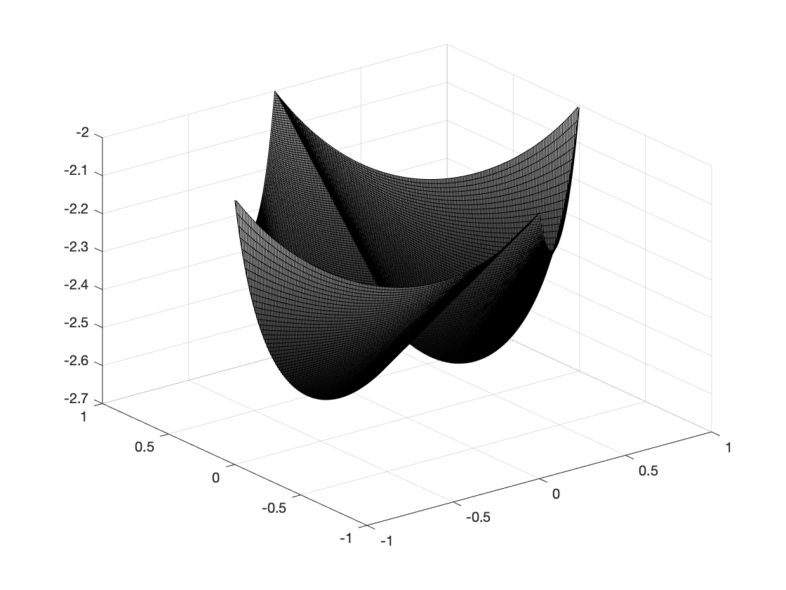
Example 4 is very illustrative in the above discussion, and thus, we conducted a detailed study of it. The first step is to observe that, since the leader’s objective is of the form , then we have that . Next, since the reaction map satisfies that , it is enough to compute in the positive quadrant part of its domain, which is given by the set . In the case of Example 4 we can give an explicit formula for in . Indeed, for every , the images of have the following form
So, by computing the centroid, we have the following Explicit formula in for the neutral value function
| (4.3) |
In Figure 4.2, the graph of of Example 4 is computed using the above explicit formula. In parallel, Figure 4.3 shows the graph of obtained by plain Monte-Carlo simulations. While the Monte-Carlo method is noisy, it clearly preserves the general shape of the function , and so, it seems to be a promising method to work with.

To find the solution of the neutral approach we used the Differential Evolution metaheuristic (see, e.g., [50]). The use of evolutionary metaheuristics in bilevel optimization is not new (see, e.g., [17] and the references therein). However, to the best of our knowledge, this is the first time that it is used to estimate the solutions of the Bayesian approach. Our method is described in Algorithm 1.
The numerical experiments were done in Matlab R2019b [36] using the open-source implementation of M. Buehren [12] for the Differential Evolution metaheuristic. We tested the algorithm with 21 linear bilevel problems of the BOLIB library (see [52] for a description of the library) and the new academic problem of Example 4. We also tested nonlinear bilevel problems from BOLIB library with linear lower-level problems (problems 24 to 27 in Table 1). We selected only the problems of BOLIB with bounded feasible region. For problems with coupling constraints, we modified them passing the constraints to the follower (which is the case only for Problem 26). The sampling size was fixed at . Results are summarized in Table 1.
| ID | Reference | (DE) | ||||
| 1 | AnandalinghamWhite1990 | 1 | 1 | 7 | -49 | -49 |
| 2 | Bard1984a | 1 | 1 | 6 | 28/9 | 3.111111 |
| 3 | Bard1984b | 1 | 1 | 6 | -37.6 | -37.6 |
| 4 | Bard1991Ex2 | 1 | 2 | 6 | -1 | -1 |
| 5 | BardFalk1982Ex2 | 2 | 2 | 7 | -3.25 | -3.25 |
| 6 | Ben-AyedBlair1990a | 1 | 2 | 6 | -2.5 | -2.5 |
| 7 | Ben-AyedBlair1990b | 1 | 1 | 5 | -6 | -6 |
| 8 | BialasKarwan1984a | 1 | 2 | 8 | -2 | -2 |
| 9 | BialasKarwan1984b | 1 | 1 | 7 | -11 | -11 |
| 10 | CandlerTownsley1982 | 2 | 3 | 8 | -29.2 | -29.2 |
| 11 | ClarkWesterberg1988 | 1 | 1 | 3 | -37 | -37 |
| 12 | ClarkWesterberg1990b | 1 | 2 | 7 | -13 | -9.5062 |
| 13 | GlackinEtal2009 | 2 | 1 | 6 | 6 | 6.0171 |
| 14 | HaurieSavardWhite1990 | 1 | 1 | 4 | 27 | 27 |
| 15 | HuHuangZhang2009 | 1 | 2 | 6 | -76/9 | -8.7778 |
| 16 | LanWenShihLee2007 | 1 | 1 | 8 | -85.09 | -85.0909 |
| 17 | LiuHart1994 | 1 | 1 | 5 | -16 | -16 |
| 18 | TuyEtal1993 | 2 | 2 | 7 | -3.25 | -3.25 |
| 19 | TuyEtal1994 | 2 | 2 | 6 | 6 | 6 |
| 21 | VisweswaranEtal1996 | 1 | 1 | 6 | 28/9 | 3.111122 |
| 22 | Example 4 | 2 | 2 | 12 | -7 | -2.61223 |
| 23 | BardBook1998Ex832 | 2 | 2 | 11 | 0 | 2.13643e-09 |
| 24 | LamparielloSagratella2017Ex35 | 1 | 1 | 5 | 0.8 | 0.8 |
| 25 | TuyEtal2007* | 1 | 1 | 5 | 22.5 | 22.5 |
| 26 | WanWangLv2011** | 2 | 3 | 8 | - | 7.500037 |
An important observation is that for any bilevel programming problem, if there exists an optimistic solution such that is a singleton, then any optimistic solution is also a Bayesian solution for any belief of the leader, in particular, for the Neutral belief. This is what occurs in most problems of BOLIB, and so, with the exception of problem 12, the exact solution of the neutral approach coincides with the value of .
In the case of Example 4, we also run a classic interior-point algorithm (implemented in the method fmincon of Matlab R2019b) in the positive quadrant, using the explicit formula of (4.3). We obtained the point as a neutral solution, with neutral value . The result of the DE heuristic for the same problem was with value . Recalling the symmetry of the problem, the results are very similar, with an error of . The errors come from the heuristic itself, but also from the noise of Monte-Carlo estimation. The overestimated value is referable to this noise and the fact that the DE metaheuristic preserves the best value, including overestimation.
5 Final comments and perspectives
In this work we extended previous existence results for bilevel problems in the Bayesian approach admitting change of dimension beyond the case of full dimension (nonempty interior of values) and null dimension (single-valued). Our existence results are based on the weak continuity of the beliefs (as decision-dependent distributions) and the rectangular continuity property, which allows to control the possible changes of affine dimension of the reaction map of the followers. Our results cover regularized problems (Corollary 1) but also (non-regularized) problems with linear lower-level (Corollary 2) or, more generally, with separable and convex weakly-analytic data in the sense of formulation (3.18). The bilevel game model we consider does not include coupling constraints, which we think would be an interesting future development of the subject.
The condition of rectangular continuity introduced in this work might seem a bit technical but really served as a tool to prove Corollary 2, which was the main motivation of the work.
An open question left by this work is whether rectangular continuity over the reaction map is in some sense minimal in order to ensure that beliefs with continuous strictly positive densities over are weak continuous. Otherwise, it would be interesting to show a counterexample or more importantly to find a more general (or an independent) condition than rectangular continuity enabling us to prove weak continuity of beliefs over .
We tested the Neutral approach (Bayesian approach with neutral belief) using a Differential Evolution metaheuristic for a family of test problems whose lower-level is linear, since we know that in this case the neutral value function is continuous. The evaluation of the value function of the neutral approach was estimated using plain Monte-Carlo integration. The obtained results are promising, since in most cases, we could compare the results with the theoretical exact solution, obtaining quite similar values. In a future work, we will further develop the algorithmic aspect of the Bayesian approach. As hinted in the Example 4, it seems that there is a stronger regularity of the value function for linear problems that needs to be explored.
The development of algorithms or heuristics to tackle the Bayesian approach remains as a perspective for this work. In particular, we would like to develop algorithms to compute solutions for both the case with one leader and the case with multiple leaders.
Acknowledgements
We thank L. Mallozzi for letting us know about her work with J. Morgan [33], which we were not aware of when the first preprint version of this work was communicated. We are also grateful to S. Dempe for his comments on the first version.
References
- [1] S. Ahmed. Strategic planning under uncertainty: Stochastic integer programming approaches. PhD thesis, University of Illinois at Urbana-Champaign, 2000.
- [2] M. J. Alves, C. H. Antunes, and J. P. Costa. New concepts and an algorithm for multiobjective bilevel programming: optimistic, pessimistic and moderate solutions. Operational Research, pages 1–34, 2019.
- [3] J.-P. Aubin and H. Frankowska. Set-valued Analysis, volume 2 of Systems & Control: Foundations & Applications. Birkhäuser Boston, Inc., Boston, MA, 1990.
- [4] C. Audet, J. Haddad, and G. Savard. A note on the definition of a linear bilevel programming solution. Applied Mathematics and Computation, 181(1):351–355, 2006.
- [5] D. Aussel and A. Svensson. Towards tractable constraint qualifications for parametric optimisation problems and applications to generalised Nash games. Journal of Optimization Theory and Applications, 182(1):404–416, 2019.
- [6] D. Aussel and A. Svensson. A short state of the art on Multi-Leader-Follower games. In Bilevel Optimization: Advances and Next Challenges, pages 53–76. Springer, 2020.
- [7] Dominique Bakry, Ivan Gentil, and Michel Ledoux. Analysis and geometry of Markov diffusion operators, volume 348 of Grundlehren der mathematischen Wissenschaften [Fundamental Principles of Mathematical Sciences]. Springer, Cham, 2014.
- [8] B. Bank, J. Guddat, D. Klatte, B. Kummer, and K. Tammer. Non-linear parametric optimization. Basel - Boston - Stuttgart: Birkhäuser Verlag, 1983.
- [9] W. Bialas and M. Karwan. Two-level linear programming. Management Science, 30(8):1004–1020, 1984.
- [10] M. Bianchi and S. Schaible. Equilibrium problems under generalized convexity and generalized monotonicity. Journal of Global Optimization, 30(2-3):121–134, 2004.
- [11] Patrick Billingsley. Convergence of probability measures. Wiley Series in Probability and Statistics: Probability and Statistics. John Wiley & Sons, Inc., New York, second edition, 1999. A Wiley-Interscience Publication.
- [12] Markus Buehren. Differential Evolution, 2021. MATLAB Central File Exchange. Retrieved August 6, 2021.
- [13] F. Caruso, M. B. Lignola, and J. Morgan. Regularization and approximation methods in stackelberg games and bilevel optimization. In Bilevel Optimization: Advances and Next Challenges, pages 77–138. Springer, 2020.
- [14] J. Cotrina, A. Hantoute, and A. Svensson. Existence of quasi-equilibria on unbounded constraint sets. Optimization, 71(2):337–354, 2020.
- [15] S. Dempe. Foundations of bilevel programming. Kluwer Academic Publishers, Dordrecht, 2002.
- [16] S. Dempe, V. Kalashnikov, G. A. Pérez-Valdés, and N. Kalashnykova. Bilevel programming problems. Theory, algorithms and applications to energy networks. Energy Systems. Springer, Heidelberg, 2015.
- [17] Stephan Dempe. Bilevel optimization: theory, algorithms, applications and a bibliography. In Bilevel Optimization: Advances and Next Challenges, pages 581–672. Springer, 2020.
- [18] Z. Dou, X. Yan, D. Wang, and X. Deng. Finding mixed strategy nash equilibrium for continuous games through deep learning, 2019. arXiv:1910.12075.
- [19] D Drusvyatskiy and L. Xiao. Stochastic optimization with decision-dependent distributions, 2020. arXiv:2011.11173.
- [20] L. C. Evans and R. F. Gariepy. Measure theory and fine properties of functions. Textbooks in Mathematics. CRC Press, Boca Raton, FL, revised edition, 2015.
- [21] F. Facchinei and C. Kanzow. Generalized Nash equilibrium problems. Annals of Operations Research, 175(1):177–211, 2010.
- [22] D. Fudenberg and J. Tirole. Game theory. MIT press, 1991.
- [23] I. L. Glicksberg. A further generalization of the Kakutani fixed theorem, with application to Nash equilibrium points. Proceedings of the American Mathematical Society, 3:170–174, 1952.
- [24] V. Goel and I. E. Grossmann. A class of stochastic programs with decision dependent uncertainty. Mathematical Programming, 108(2-3, Ser. B):355–394, 2006.
- [25] J. Harsanyi. Games with incomplete information played by “bayesian” players, i–iii part i. the basic model. Management Science, 14(3):159–182, 1967.
- [26] M. Hu and M. Fukushima. Multi-leader-follower games: models, methods and applications. Journal of the Operations Research Society of Japan, 58(1):1–23, 2015.
- [27] T. Ichiishi. Game theory for economic analysis. Economic Theory, Econometrics, and Mathematical Economics. Academic Press, Inc. [Harcourt Brace Jovanovich, Publishers], New York, 1983.
- [28] S. Jia, Z. Wan, Y. Feng, and G. Wang. New partial cooperation model for bilevel programming problems. Journal of Systems Engineering and Electronics, 22(2):263–266, 2011.
- [29] T. W. Jonsbråten, R. J.-B. Wets, and D. L. Woodruff. A class of stochastic programs with decision dependent random elements. Annals of Operations Research, 82:83–106, 1998.
- [30] A. Klenke. Probability Theory: A Comprehensive Course. Springer, 2014.
- [31] Gunther Leobacher and Friedrich Pillichshammer. Introduction to quasi-Monte Carlo integration and applications. Compact Textbooks in Mathematics. Birkhäuser/Springer, Cham, 2014.
- [32] J. Liu, Y. Fan, Z. Chen, and Y. Zheng. Pessimistic bilevel optimization: a survey. International Journal of Computational Intelligence Systems, 11(1):725–736, 2018.
- [33] L. Mallozzi and J. Morgan. Hierarchical Systems with Weighted Reaction Set, pages 271–282. Springer US, Boston, MA, 1996.
- [34] L. Mallozzi and J. Morgan. Oligopolistic markets with leadership and demand functions possibly discontinuous. Journal of Optimization Theory and Applications, 125(2):393–407, 2005.
- [35] M. A. Mansour and D. Aussel. Quasimonotone variational inequalities and quasiconvex programming: qualitative stability. Journal of Convex Analysis, 15(3):459, 2008.
- [36] The Mathworks, Inc., Natick, Massachusetts. MATLAB version R2019b, 2021.
- [37] A. G. Mersha and S. Dempe. Linear bilevel programming with upper level constraints depending on the lower level solution. Applied Mathematics and Computation, 180(1):247–254, 2006.
- [38] E. Michael. Continuous selections. I. Annals of Mathematics, pages 361–382, 1956.
- [39] J. F. Nash. Non-cooperative games. Annals of Mathematics. Second Series, 54:286–295, 1951.
- [40] O. Nohadani and K. Sharma. Optimization under decision-dependent uncertainty. SIAM Journal on Optimization, 28(2):1773–1795, 2018.
- [41] J.-S. Pang and M. Fukushima. Quasi-variational inequalities, generalized Nash equilibria, and multi-leader-follower games. Computational Management Science, 2(1):21–56, 2005.
- [42] Christos H. Papadimitriou. The complexity of finding Nash equilibria. In Algorithmic game theory, pages 29–51. Cambridge Univ. Press, Cambridge, 2007.
- [43] S. Peeta, F. S. Salman, D. Gunnec, and K. Viswanath. Pre-disaster investment decisions for strengthening a highway network. Computers & Operations Research, 37(10):1708–1719, 2010.
- [44] D. Pereda. Modeling and analysis of electricity auctions. Master’s thesis, Universidad de Chile, 2019.
- [45] C. C. Pugh. Real mathematical analysis. Springer, 2002.
- [46] R. T. Rockafellar and R. J.-B. Wets. Variational Analysis, volume 317. Springer Science & Business Media, 2009.
- [47] S. Tadelis. Game Theory: An Introduction. Princeton University Press, Princeton, NJ, 2013.
- [48] H. Von Stackelberg. Marktform und Gleichgewicht. Springer, 1934.
- [49] Larry Wasserman. All of statistics: a concise course in statistical inference, volume 26. Springer, 2004.
- [50] Xin-She Yang. Nature-inspired optimization algorithms. Elsevier, Inc., Amsterdam, 2014.
- [51] Y. Zheng, D. Fang, and Z. Wan. A solution approach to the weak linear bilevel programming problems. Optimization, 65(7):1437–1449, 2016.
- [52] S. Zhou, A. B. Zemkoho, and A. Tin. BOLIB: Bilevel optimization library of test problems. In Bilevel Optimization: Advances and Next Challenges, pages 563–580. Springer, 2020.