Reinforcement Learning on Computational Resource Allocation of Cloud-based Wireless Networks
Abstract
Wireless networks used for Internet of Things (IoT) are expected to largely involve cloud-based computing and processing. Softwarised and centralised signal processing and network switching in the cloud enables flexible network control and management. In a cloud environment, dynamic computational resource allocation is essential to save energy while maintaining the performance of the processes. The stochastic features of the Central Processing Unit (CPU) load variation as well as the possible complex parallelisation situations of the cloud processes makes the dynamic resource allocation an interesting research challenge. This paper models this dynamic computational resource allocation problem into a Markov Decision Process (MDP) and designs a model-based reinforcement-learning agent to optimise the dynamic resource allocation of the CPU usage. Value iteration method is used for the reinforcement-learning agent to pick up the optimal policy during the MDP. To evaluate our performance we analyse two types of processes that can be used in the cloud-based IoT networks with different levels of parallelisation capabilities, i.e., Software-Defined Radio (SDR) and Software-Defined Networking (SDN). The results show that our agent rapidly converges to the optimal policy, stably performs in different parameter settings, outperforms or at least equally performs compared to a baseline algorithm in energy savings for different scenarios.
Index Terms:
Reinforcement learning, IoT, Cloud, SDN, SDR, Markov Decision ProcessI Introduction
Cloud-based systems have been proposed and implemented for many promising IoT (IoT) applications, such as smart city and e-health [1, 2]. Two enabling technologies, SDR (SDR) and SDN (SDN), recently started to be utilised in the cloud to support the virtualisation of the IoT network [3]. In a cloud environment, computational resources (e.g. CPU, memory, and storage) are virtualised and allocated to fulfil the requirements of different IoT services. Optimising computational resource allocation in the cloud to balance energy consumption and processing performance is an important research topic. Reinforcement learning provides an effective method for solving such an optimisation problem in a stochastic and dynamic environment.
In this paper, we design and implement a model-based reinforcement-learning agent based on MDP (MDP), to intelligently allocate computational resources for cloud-based wireless networks. The agent analyses the state transition probabilities between different states, reflecting different levels of CPU (CPU) utilisation, as well as the corresponding reward functions, and then decides to either remain in the same state or to change states by adding/reducing one CPU core. The reward function for each state-action pair drives the agent to optimise the total reward after multiple MDP steps. We use a value iteration algorithm [4] for the agent to solve this MDP and arrive at an optimal policy that balances the energy savings and cloud performance.
We simulate many different SDR and SDN scenarios to evaluate the performance of our reinforcement-learning agent. We have found that the optimal policies carried out by the agent are different for SDR or SDN cases. The results show that our agent with value iteration outperforms a baseline algorithm in terms of energy savings in some of the scenarios while achieving similar performance in the other scenarios. We also investigate the performance of our agent with different transition probabilities as well as a higher number of MDP states to verify the scalability of our agent.
Our contribution in this paper can be summarised as follows: 1) the modelling of the dynamic CPU resource allocation problem in the cloud-based wireless networks by MDP; 2) the utilisation of value iteration method to solve the MDP to get the optimal policy; and 3) the comprehensive analysis of the performance of our reinforcement learning agent in various scenarios with different parameters.
II Background and related work
Reinforcement learning was originally invented for robotics and automation. Recently with the artificial intelligence and machine learning being introduced to broader research areas, reinforcement learning has started to be applied in communications and networking. The main advantage of reinforcement learning is that it does not need a large dataset during the training process. A reinforcement-learning agent is capable to sense the environment and learn to make decisions by itself during the training. To design a reinforcement learning agent, a description of the environment is essential, either mathematically modelled as an input to the agent (i.e., model-based), or learnt by the agent itself (i.e., model-free). In this paper we model the cloud computational resource allocation problem as an MDP, which is a commonly used model to describe a stochastic process [4]. We then get optimal solutions for the agent by value iteration, which is an effective reinforcement-learning algorithm to solve the MDP.
There are some recent works published on reinforcement learning utilisation on the computational resource allocation and offloading at the edge computing or fog computing. For instance, authors in [5] used reinforcement learning to optimise the computational task offloading problem from mobile users to edge computing servers. The authors in [6] proposed a reinforcement-learning method to offload the computational task from one user to another user in ad-hoc wireless networks with MDP model. Besides, authors in [7] applied MDP to model the container migration problem in fog computing and then use reinforcement learning to design an agent that migrates containers between different physical servers while optimising the total power consumption. Despite the fact that reinforcement learning has been used for addressing many different resource or task allocation problems in cloud computing, to the best of our knowledge, our work is the first one that investigates the problem of dynamic CPU resource allocation of cloud-based wireless networks by reinforcement learning.
III System Model
In this section we first describe the MDP model that we build for the dynamic computational resource allocation problem of cloud-based wireless networks. After that we define the reward function, value function and Q function for this MDP model, as the parameters for our reinforcement-learning agent. Finally we present the value iteration algorithm that can help solve the MDP model and get optimal policies by reinforcement learning.
III-A The MDP model
MDP is a discrete-time stochastic process that is used for modelling the decision making procedure involving multiple states and actions in a stochastic environment [8]. According to our observation of the statistics of Trinity College Dublin’s cloud-based Iris testbed [9], we model the stochastic process of the CPU usage and the CPU allocation of cloud processes in our testbed as an MDP. Supposing denotes the maximum instant CPU load percentage for the cores that are being used (e.g., if a container in the cloud is using 3 CPU cores with the load percentage of 50%, 60% and 70%, ), the core with becomes the bottle neck of the container in terms of the processing performance. We then categorise the CPU load percentage into three levels, i.e., low utilisation state (), medium utilisation state () and high utilisation state (), corresponding to the three states in the MDP. Note that we have also made the cases with more states (i.e., more fine-grained categorisation of CPU load percentage levels) later on in the result section and proved that the results with more states are similar with the three states case.
After defining the states, we define the three options of actions for the reinforcement-learning agent in the MDP to be 1) keeping the current CPU numbers, i.e., ; 2) adding one CPU core, i.e., ; 3) reducing one CPU core, i.e., . The transitions between the states ’s after operating the action ’s are stochastic processes due to the uncertainty of the parallelisation situations of the processes running on the CPU cores, i.e., adding or reducing one CPU core would not necessarily change the states. We define the state transition probability as the probability of getting into the next state (either the same one or a different one) if taking action from state . We also define the reward of this transition as , as the parameter for our reinforcement learning agent. The time interval of the agent taking the actions can be customised to be different levels (e.g. in seconds, in minutes or in hours) depending on the needs of the network administrators.

Figure 1 illustrates the state transition diagram of the aforementioned MDP model, including the 3 states, i.e. , (low CPU load percentage), (medium CPU load percentage) and (high CPU load percentage), as well as the 3 actions, i.e., (doing nothing), (adding one CPU core) and (reducing one CPU core). The figure also shows the transition probabilities as well as the corresponding rewards with the arrowed lines between the states and actions. Different colours of arrowed lines are only for improving visibility. Note that taking action from state is not considered because it is not realistic to reduce one CPU core when the CPU load percentage is already high.
III-B Reward function, Value function, and Q function
In this subsection we define the reward function, value function and Q function from this MDP for the reinforcement learning [4]. The objective of solving this MDP is to find a policy that maximises the total reward when the system transits between the states after certain MDP steps . The total reward follows Equation (1) where denotes the reward of each time step and is the discount factor (, set to be 0.9 in this paper) that avoids the total reward going to infinity [4].
| (1) |
We then define the value function of each state , denoting the expected total reward for an agent starting from state with the policy (shown in Equation (2)). In this way, indicates how good the state is for an agent to stay. Among all policy ’s, there existing an optimal policy that makes to be maximum (shown in Equation (3)) [4].
| (2) |
| (3) |
We then define as the short version for from now on for simplicity. In order to get the optimal , in reinforcement learning, the agent needs to try all policy ’s that include all possible combinations of state-action pairs . The Q function for each state-action pair can be defined to indicate how beneficial it is for the agent to use action when in the state . Therefore the maximum value of () equals to the maximum value of () for all the possible action ’s (shown in Equation (4)) [4].
| (4) |
According to the Bellman Equation [10], The optimal equals to the summation of 1) the expectation of immediate reward after taking action from state (considering all possible next states ’s) and 2) the discounted expectation of all future maximum rewards (for all possible next states ’s as well), shown in Equation (5) [4].
| (5) |
Therefore, according to Equation (4) and (5), we can derive Equation (6), for all possible state ’s transiting from state taking action [4].
| (6) |
III-C Reinforcement learning and value iteration
According to the aforementioned Equations (2)-(6), the reinforcement learning agent needs to obtain the maximum and the corresponding optimal policy to perform an optimal solution to this MDP. Assuming and are both known for all the triple tuples , we can use a reinforcement learning method, namely value iteration algorithm, to solve the optimal , by a recursive method using Equation (6). The pseudo code of the value iteration algorithm can be expressed as the following Algorithm 1 [4]:
The value iteration algorithm first initialises the value function with arbitrary values (in our case, zeros), and then updates it with the value of the latest Q function when making a step ahead. After a number of iterations the value function converges to the optimal value , when the difference between the last two iterations is less than a very small value . The corresponding policy becomes the optimal policy (i.e., the optimal state-action pairs ).
IV Experimental results
To evaluate the performance of our agent running the aforementioned value iteration algorithm in a cloud-based wireless network scenario, we investigate two commonly-used network processes, i.e., SDN and SDR. We conduct our simulations with different experimentation parameters and compare the results with another baseline algorithm.
IV-A Definition of transition probabilities and rewards of MDP
We start with an experiment of 3 states for the MDP (shown in Figure 1). We define the parameters we use for the MDP simulation for both SDN and SDR cases in Table I. The transition probabilities between the 3 states (i.e., 3 levels of CPU core usage percentage) are derived from the general experimental data statistics of the Trinity College Dublin Iris testbed [9]. The SDN and SDR cases have different transition probabilities, due to the facts that 1) a single SDN process utilises a lower percentage of a CPU core but there are usually multiple processes running at the same time to share the same CPU core, meaning that SDN processes are more likely to be parallelised; 2) a single SDR process utilises a higher percentage of a CPU core and is usually not capable to be parallelised. Therefore, the probability for SDN to transit to other states is larger than the one for SDR when increasing or decreasing the number of allocated CPU cores.
Besides, we define the normalised rewards of the reinforcement learning procedure when solving the MDP (also shown in Table I). The definition of the rewards is based on the objective that is to minimise the total number of running CPU cores (to save energy) while avoiding long-term high CPU load percentage (to guarantee the overall performance of the cloud system). In general, the reward is positive when 1) reducing one CPU core and the CPU load keeps the same level; or 2) adding one CPU core and the CPU load level gets lower. The reward is negative when 1) doing nothing (i.e. with action ); or 2) adding one CPU core but CPU load level remains; or 3) reducing one CPU core and CPU load level increases.
| Transition probabilities | Rewards | |||
|---|---|---|---|---|
| SDN | SDR | SDN & SDR | ||
| 1 | 1 | -3 | ||
| 1 | 1 | -5 | ||
| 0.3 | 0.7 | +5 | ||
| 0.7 | 0.3 | -5 | ||
| 1 | 1 | -1 | ||
| 0.8 | 0.2 | +5 | ||
| 0.2 | 0.8 | -5 | ||
| 0.3 | 0.7 | +5 | ||
| 0.7 | 0.3 | -5 | ||
| 1 | 1 | -5 | ||
| 0.8 | 0.2 | +5 | ||
| 0.2 | 0.8 | -5 | ||
IV-B Results with 3 states, certain transition probability and predefined rewards
As mentioned in the previous section, we design the reinforcement-learning agent to find the optimal policy using the value iteration algorithm (Algorithm 1). We use Python 3.5 open-source MDP library [11] to implement the MDP model, the value iteration procedure and simulation of the results. The threshold of the convergence ( in the Algorithm 1) is set to be a very small value (). The value iteration algorithm converges rapidly to optimal values. For SDN case it converges after 66 iterations, while for SDR case it converges after 56 iterations.
Figure 2 and Figure 3 show the value function variations and convergence during the value iteration process for SDR and SDN respectively. For the case of SDR there is when converged; while for the case of SDN there is when converged. The results mean that in the case of SDR the agent prefers to go for a lower CPU load state, while in the case of SDN the agent prefers to go for a higher CPU load state. To understand the decision of the agent, we should take into account the fact that the SDN processes are easier to be parallelised than the SDR processes, therefore it is safer to push to a higher CPU load state for SDN to save resources than SDR, because in the case of SDN adding one CPU will more likely bring down the high CPU load and get positive reward. However for the SDR case the states tend to stay when adding/reducing CPUs therefore there is a higher risk for the agent to stay in the high CPU load state and get continuously high penalties.
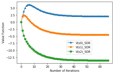
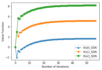
Besides, the agent also derives the optimal policy denoted by state-action pairs . For the case of SDR they are , , and , while for the case of SDN they are , , and . These two cases have the same optimal actions at the state and , which are and respectively, meaning that the agent chooses to reduce one CPU when the CPU load is low and to add one CPU when the CPU load is high, which is straightforward to understand since these two actions are the only options in these two states to get an immediate positive reward. However, the optimal action for the medium state is different for SDR and SDN, For the case of SDR the agent prefers to reduce one CPU at the state of while for the case of SDN the agent prefers to add one CPU at the state of . These two decisions are not obvious to understand since both actions on state can make the same immediate reward. Therefore the agent has to decide these actions not only by the immediate reward, but also by maximising the total reward considering future rewards with the discount factor (see Equation (1)). These decisions are optimised by the value iteration.
IV-C Results with different transition probabilities
In the previous subsection, we obtain the transition probabilities shown in Table I based on the general statistics of the Trinity College Dublin Iris testbed [9]. In this subsection we change these probabilities and see how the changes would effect to the results, to further evaluate the scalability of our algorithm to other testbeds/scenarios. We keep those probability values that equal to 1 in Table I for the cases in which state transition is definite, and vary the other ”not-equal-to-1” values that are for the transition probability between different states. We assume that for the SDR case those values vary among 0.01, 0.1, 0.2, 0.3, and 0.4, while for the SDN case those values vary among 0.6, 0.7, 0.8, 0.9 and 0.99. The reason is that SDN processes are more likely to be parallelised thus more likely to transit to another state when adding/reducing one CPU core.
The results in Figure 4 show the relation between the aforementioned state transition probability from one state to another state (X axis) and the standard deviation of the value functions of the 3 states (Y axis). The results show that the variation of transition probabilities affects a lot to the standard deviation of the value functions for the SDR case but not so much for the SDN case. Besides, the curves for the SDR and SDN cases show different tendencies with the increasing of transition probability. In general, higher standard deviation of value functions means the reinforcement-learning agent has more obvious preferences on different states. In Figure 4 we also plot the case for equal probability values (i.e. with 0.5 transition probability, meaning equal probability to stay in the same state or to transit to another state), in which case the state value functions all equal to 0 (). This means that the agent is indifferent to the 3 different states therefore the value iteration does not work properly in this case.

IV-D Results compared to other algorithms
In this subsection, we compare the results of our value iteration algorithm with another baseline algorithm. According to the previous analysis and review values in Table I, for the states or there is only one optimal choice of state-action pair, (i.e., or ), which has positive reward value. Therefore any optimisation algorithm would choose these two state-action pairs. However, the difference occurs when transiting from the state , where there is no obvious preference for the agent on taking the action or in terms of immediate rewards. The benefit of the algorithm will appear with time goes by. Therefore, to compare the performance of our algorithm and the baseline algorithm, we simulate the MDP procedure to calculate the cumulative reward (defined by Equation 1) after a certain number of MDP steps.
We define the baseline algorithm, namely RAS (RAS) algorithm, to compare with our value iteration algorithm. The RAS algorithm randomly chooses the action or made at the state with equally 50% probability respectively. Figure 5 shows the comparison of cumulative reward between our value iteration approach and the RAS approach for one single time-based MDP simulation. The simulation is conducted under the same SDR case with the state transition probability equal to 0.1 for both adding one CPU and reducing one CPU. The results show that our agent with value iteration gets more cumulative reward during the reinforcement learning process than the agent with RAS, meaning our agent works more efficiently to reach our goal.

We also build simulations to compare the energy savings and CPU working performance for value iteration and RAS algorithm, in a cloud with 1000+ available CPU cores. Instead of showing the results for a single MDP as Figure 5, we build 10000 independent MDP simulations with each simulation having 1000 MDP steps and take average results to get more reliable comparisons.
To showcase the energy savings, Figure 6 shows the comparison between value iteration and RAS for total number of added/reduced CPU cores in different transition probability cases (positive numbers on Y-axis mean adding CPUs while negative numbers mean reducing CPUs). Besides, to showcase the performance maintenance, Figure 7 shows the comparison between value iteration and RAS for percentage of time in high CPU load state () in different transition probability cases.
By looking at Figure 6, for SDR case, our agent with value iteration reduces more number of CPU cores in the MDP than RAS, especially for cases where transition probability is less than 0.2. This means that our agent saves more energy than the baseline RAS in the cloud systems for the SDR case. For instance, for the case where transition probability equals to 0.01, our value iteration agent saves energy consumption of 40 more CPUs than RAS does. If one high-performance CPU core consumes 80 watts [12], saving 40 CPUs corresponds to around 76.8 kWh energy savings per day. However, Figure 7 shows that value iteration has around 25% more time in high-load CPU state than RAS in SDR cases (although it is still below 50% of time), meaning that our agent takes higher risk on keeping the CPUs on high-load states than RAS. For SDN case, our agent with value iteration has similar CPU core reductions (i.e. energy savings) as RAS, but takes lower risk on keeping the CPUs on high-load states than RAS. Note that we don’t consider the case in which the transition probability equals to 0.5 on the X-axis because in this case the value iteration does not work properly (as mentioned in Figure 4).


IV-E Results with more states
In this subsection, we investigate the case with more MDP states (4 states) and see if the results follow the similar trend, to evaluate the scalability of our agent using value iteration when the CPU-usage levels are defined to be more fine-grained. To make the case for “4 states” we add one more intermediate state to the previous 3-state scenario shown in Figure 1, between the low-CPU-usage state and high-CPU-usage state (becoming after adding one state) while keeping the same structure of actions ’s, transition probabilities and rewards. We conduct the experiments on the 4-state scenario with the same transition probabilities and reward parameters as the 3-state scenario. The results show the same trend as Figure 2 and Figure 3. The number of iterations to reach convergence is also around 60. For the SDR case the value functions follow , while for the SDN case the value functions follow . Besides, the optimal state-action pair selections for the 4-state case are the same as the 3-state case as well. We are not showing the figures here due to the page limits. These results mean that our agent with value iteration is extendable to scenarios with more states and more fine-grained CPU levels.
V Conclusion and future work
In this paper, we have designed and implemented an MDP-based model to represent the dynamic CPU resource allocation problem in cloud-based wireless networks. We use value iteration algorithm to build a reinforcement learning agent to get the optimal policy. We have investigated different scenarios with different parameters as well as comparing the performance with another baseline algorithm, namely RAS. From the simulation results we have found that our agent gets the optimal policy rapidly in under 100 iterations and the algorithm are extendable to many different scenarios. Our agent with value iteration outperforms or at least equally performs in energy savings compared to the baseline algorithm.
In this paper, we predefined the transition probabilities in the MDP according to the statistics, which means that the agent is fully aware of the environment. In future, we plan to build more sophisticated reinforcement learning scenarios where the agent is not fully aware of the environment, and has to update its optimal decisions with time goes by. These will involve deep Q-learning techniques with neural networks.
- 3GPP
- Third Generation Partnership Project
- ASIC
- Application-specific Integrated Circuit
- ANN
- Artificial Neural Network
- BBU
- Baseband Unit
- C-RAN
- Cloud Radio Access Network
- CPU
- Central Processing Unit
- C-RANs
- Cloud Radio Access Networks
- D-RAN
- Distributed Radio Access Network
- DNN
- Deep Neural Network
- FDD
- Frequency Division Duplex
- FTTx
- Fibre To The x
- GPP
- General Purpose Processor
- HD
- High Definition
- IoT
- Internet of Things
- LTE
- Long Term Evolution
- LXC
- Linux Container
- MCS
- Modulation and Coding Scheme
- MDP
- Markov Decision Process
- NFV
- Network Function Vitualisation
- OFDM
- Orthogonal Frequency Division Multiplexing
- OLT
- Optical Line Terminal
- ONU
- Optical Network Unit
- OTT
- Over-the-top
- PHY
- Physical
- PON
- Passive Optical Networks
- PRB
- Physical Resource Block
- QAM
- Quadrature Amplitude Modulation
- RAS
- Random-Action-Selection
- RRH
- Remote Radio Head
- SDN
- Software-Defined Networking
- SDR
- Software-Defined Radio
- TBS
- Transport Block Size
- TDM
- Time Division Multiplexing
- vBBU
- virtual Baseband Unit
- VNO
- Virtual Network Operator
- vOLT
- vitual Optical Line Terminal
- WDM
- Wavelength Division Multiplexing
- UE
- User Equipment
Acknowledgement
This publication has emanated from the research supported by the European Commission Horizon 2020 under grant agreements no. 732174 (ORCA), and co-funded under the European Regional Development Fund from Science Foundation Ireland under Grant Number 13/RC/2077 (CONNECT). This material is also based on works supported by Science Foundation Ireland under Grant No. SFI/12/RC/2289_P2.
References
- [1] B. V. Natesha and R. M. R. Guddeti, “Heuristic-Based IoT Application Modules Placement in the Fog-Cloud Computing Environment,” in 2018 IEEE/ACM International Conference on Utility and Cloud Computing Companion (UCC Companion), Dec 2018, pp. 24–25.
- [2] K. Monteiro, E. Rocha, E. Silva, G. L. Santos, W. Santos, and P. T. Endo, “Developing an e-Health System Based on IoT, Fog and Cloud Computing,” in 2018 IEEE/ACM International Conference on Utility and Cloud Computing Companion (UCC Companion), Dec 2018, pp. 17–18.
- [3] T. Ahmed, A. Alleg, and N. Marie-Magdelaine, “An Architecture Framework for Virtualization of IoT Network,” in 2019 IEEE Conference on Network Softwarization (NetSoft), June 2019, pp. 183–187.
- [4] R. S. Sutton and A. G. Barto, Reinforcement Learning: An Introduction. MIT Press, 2018.
- [5] J. Li, H. Gao, T. Lv, and Y. Lu, “Deep reinforcement learning based computation offloading and resource allocation for MEC,” in 2018 IEEE Wireless Communications and Networking Conference (WCNC), April 2018, pp. 1–6.
- [6] D. Van Le and C. Tham, “A deep reinforcement learning based offloading scheme in ad-hoc mobile clouds,” in IEEE INFOCOM 2018 - IEEE Conference on Computer Communications Workshops (INFOCOM WKSHPS), April 2018, pp. 760–765.
- [7] Z. Tang, X. Zhou, F. Zhang, W. Jia, and W. Zhao, “Migration Modeling and Learning Algorithms for Containers in Fog Computing,” IEEE Transactions on Services Computing, pp. 1–1, 2018.
- [8] R. Bellman, “A Markovian Decision Process,” Indiana Univ. Math. J., vol. 6, pp. 679–684, 1957.
- [9] CONNECT centre. Iris - The Reconfigurable Testbed. Accessed: Jan. 2020. [Online]. Available: https://iris-testbed.connectcentre.ie/
- [10] R. E. Bellman, Dynamic Programming. New York, NY, USA: Dover Publications, Inc., 2003.
- [11] S. Russell and P. Norvig. Artificial Intelligence: A Modern Approach . Accessed: Jan. 2020. [Online]. Available: http://aima.cs.berkeley.edu/python/mdp.html
- [12] Intel. Intel Core processors. Accessed: Jan. 2020. [Online]. Available: https://www.intel.com/content/www/us/en/products/processors/core.html