Light Field Salient Object Detection:
A Review and Benchmark
Abstract
Salient object detection (SOD) is a long-standing research topic in computer vision and has drawn an increasing amount of research interest in the past decade. Since light fields record comprehensive information of natural scenes that benefit SOD in a number of ways, using the light field inputs to improve saliency detection over conventional RGB inputs is an emerging trend. This paper provides the first comprehensive review and benchmark for light field SOD, which has long been lacking in the saliency community. Firstly, we introduce preliminary knowledge on light fields, including theory and data forms, and then review existing studies on light field SOD, covering ten traditional models, seven deep learning-based models, one comparative study, and one brief review. Existing datasets for light field SOD are also summarized with detailed information and statistical analyses. Secondly, we benchmark nine representative light field SOD models together with several cutting-edge RGB-D SOD models on four widely used light field datasets, from which insightful discussions and analyses, including a comparison between light field SOD and RGB-D SOD models, are achieved. Besides, due to the inconsistency of datasets in their current forms, we further generate complete data and supplement focal stacks, depth maps and multi-view images for the inconsistent datasets, making them consistent and unified. Our supplemental data makes a universal benchmark possible. Lastly, because light field SOD is quite a special problem attributed to its diverse data representations and high dependency on acquisition hardware, making it differ greatly from other saliency detection tasks, we provide nine hints into the challenges and future directions, and outline several open issues. We hope our review and benchmarking could help advance research in this field. All the materials including collected models, datasets, benchmarking results, and supplemented light field datasets will be publicly available on our project site https://github.com/kerenfu/LFSOD-Survey.
Index Terms:
Light field, salient object detection, deep learning, benchmarking.I Introduction
In Google I/O 2021 held in May, Google just introduced its new technology called Project Starline11 1 https://blog.google/technology/research/project-starline/, which combines specialized hardware and computer vision technology to create a “magic window” that can reconnect two remote persons, making them feel as if they are physically sitting in front of each other in the conversation. Such immersive technology, is benefited from light field display, and does not require additional glasses or headsets. The three crucial techniques involved therein, include 3D imaging, real-time data compression, and light field-based 3D display, which are very challenging but have had certain breakthroughs according to Google. In this regard, salient object detection (SOD) from the light field may be another effective way [1] to benefit these three stages.
Salient object detection (SOD) [2, 3, 4] is a fundamental task in computer vision, aiming at detecting and segmenting conspicuous regions or objects in a scene, whereas light field SOD [5, 6] studies the problem of how to realize SOD using light field data. Numerous applications of SOD cover, e.g., object detection and recognition [7, 8, 9, 10, 11], semantic segmentation [12, 13, 14], unsupervised video object segmentation [15, 16], multimedia compression [17, 18, 19, 20], non-photorealist rendering [21], re-targeting [22], and also human-robot interaction [23, 24]. Generally, the abundant cues and information within the light field help algorithms better identify target objects and advance SOD performance comparing to the conventional SOD task that processes single-colour images [25, 26, 27, 28, 29].

Light field SOD explores how to detect salient objects using light field data as input. In the 3D space, a light field [37] captures all the light rays at every spatial location and in every direction. As a result, it can be viewed as an array of images captured by a grid of cameras. Compared with the RGB images captured by a regular camera or depth maps acquired by a depth sensor, the light field data acquired by a plenoptic camera records more comprehensive and complete information of natural scenes, covering, for example, depth information [38, 39, 40, 41, 42, 43, 44], focusness cues [42, 5] as well as angular changes [42, 45]. Therefore, light field data can benefit SOD in a number of ways. Firstly, light fields can be refocused after being acquired [42]. This enables a stack of images focusing on different depths to be produced, providing focusness cues that have been demonstrated useful for SOD [46]. Secondly, a light field can provide images of a scene from an array of viewpoints [47]. Such images have abundant spatial parallax and geometric information. Lastly, the depth information of a scene is embedded in light field data and can be estimated from a focal stack or multi-view images by different means, as described in [38, 39, 40, 41]. In this sense, RGB-D data could be deemed as a special degenerated case of light field data. Fig. 1 shows example results obtained using light field SOD methods on light field data (a focal stack), as well as RGB-D SOD models on depth data, respectively.
Although light field data brings great benefits to SOD and this task first emerged in 2014 [5], it still remains somewhat under-explored. Specifically, compared with RGB SOD or RGB-D SOD, there are fewer studies on light field SOD. Despite this sparsity of literature, existing models vary in technical frameworks as well as light field datasets used. However, to the best of our knowledge, there is no comprehensive review or benchmark for light field SOD. Although a comparative study was conducted by Zhang et al. [48] in 2015, they only compared the classic light field SOD model proposed by Li et al. [5] with a set of 2D saliency models to demonstrate the effectiveness of incorporating light field knowledge. Besides, the evaluation was conducted on the LFSD dataset, which only contains 100 light field images. Recently, Zhou et al. [49] briefly summarized existing light field SOD models and related datasets. However, their work was mainly focused on RGB-D based SOD, and only a small portion of content and space was dedicated to reviewing light field SOD, leading to an insufficient review of model details and related datasets. Besides, they did not benchmark light field SOD models or provide any performance evaluation. Thus, we believe that the lack of a complete review of the existing models and datasets may hinder further research in this field.
To this end, in this paper, we conduct the first comprehensive review and benchmark for light field SOD. We review previous studies on light field SOD, including ten traditional models [5, 50, 30, 51, 52, 53, 1, 54, 55, 56], seven deep learning-based models [57, 45, 31, 32, 58, 59, 60], one comparative study [48], and one brief review [49]. In addition, we also review existing light field SOD datasets [5, 53, 57, 45, 59], and provide statistical analyses for them, covering object size, the distance between the object and image center, focal slice number, and a number of objects. Due to the inconsistency of datasets (for example, some do not provide focal stacks, while others lack depth maps or multi-view images), we further generate and complete data, including focal stacks, depth maps and multi-view images for several datasets, therefore making them consistent and unified. Besides, we benchmark nine light field SOD models [5, 50, 30, 54, 45, 32, 31, 58, 59] whose results/codes are available, together with several cutting-edge RGB-D SOD models [35, 33, 61, 62, 63, 64, 65, 66, 36], discussing the connection between the two and providing insight into the challenges and future directions. All the materials involved in this paper, including collected models, benchmark datasets, and results, supplemental light field data, and source code links, will be made publicly available on https://github.com/kerenfu/LFSOD-Survey. The main contributions of this paper are four-fold:
- •
We provide the first systematic review on light field SOD, including models and datasets. Such a survey has long been lacking in the saliency community and is helpful for encouraging future research in this area.
- •
We conduct analyses on the properties of different datasets. As some datasets lack certain forms of data, e.g., focal stacks, or multi-view images, we generate more data from existing datasets as a supplement, making them complete and unified. This will also facilitate future research in this area.
- •
We further benchmark nine light field SOD models together with several cutting-edge RGB-D SOD models on the datasets with our supplemental data, and provide insightful discussions.
- •
We investigate several challenges for light field SOD and discuss its relation to other topics, shedding light on the challenges and directions for future work.
The remainder of the paper is organized as follows. We review light field preliminaries, existing models and datasets for light field SOD, and provide related discussions and analyses in Section II. In Section III, we describe the evaluation metrics used as well as benchmark results. We then discuss future research directions and outline several open issues of this field in Section IV. Finally, we draw conclusion in Section V.
II Preliminaries, Models and Datasets
In this section, we first briefly introduce the theory of light field, the data forms of it, and how it has been used for SOD. We then review the previous works on light field SOD, roughly categorizing them into traditional models and deep learning-based models. Finally, we summarize datasets explored for light field SOD and review their detailed information.

II-A Light Field
II-A1 Light Field and Light Field Cameras
A light field [37] consists of all the light rays flowing through every point and in every direction of the 3D space. In 1991, Adelson and Bergen [67] proposed a plenoptic function (), which uses to describe the wavelength and time in any direction at any point , in order to represent the light field information. In an imaging system, the wavelength and time can be represented by RGB channels and different frames, and light usually propagates along a specific path. As a result, Levoy and Hanrahan [68] proposed the two-plane parameterization of the plenoptic function to represent the light field in an imaging system. The two-plane parameterization () of the plenoptic function, illustrated in Fig. 2 (b), can be formulated as . In this scheme, each ray in the light field is determined by two parallel planes to represent spatial and angular information. Based on this theory, devices that can capture light fields were invented, namely the Lytro cameras shown in Fig. 2 (a). This kind of camera contains the main lens and a micro-lens array placed before the photosensor, where the former serves as the “” plane, which records the angular information of rays, and the latter serves as the “” plane, which records the spatial information. Fig. 2 (b) shows the graphical representation of the two-plane parameterization for the light field. Due to the above four-dimensional parameterization, data from such a light field is often called 4D light field data [5, 50, 30, 51, 52, 6, 53, 1, 54, 55, 57, 45, 31, 32, 58, 59, 60, 48, 56].
II-A2 Forms of Light Field Data
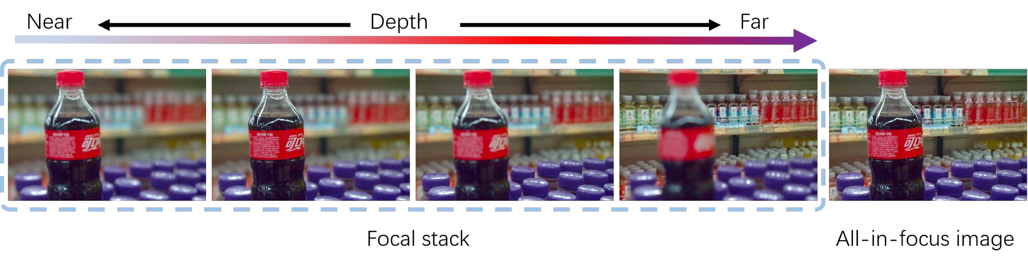
Up to now, all public light field datasets for SOD have been captured by Lytro cameras, the raw data of which are LFP/LFR files (the former are obtained from Lytro whereas the latter are from Lytro Illum). All images in the current light field datasets were generated by processing LFP/LFR files using Lytro Desktop software22 2 http://lightfield-forum.com/lytro/lytro-archive/ or LFToolbox33 3 http://code.behnam.es/python-lfp-reader/ and also https://ww2.mathworks.cn/matlabcentral/fileexchange/75250-light-field-toolbox. Since the raw data can hardly be utilized, the data forms of light fields leveraged by existing SOD models are diverse, including focal stacks plus all-in-focus images [5, 50, 30, 52, 53, 1, 54, 55, 45, 31, 32, 58], multi-view images plus center-view images [45, 53, 60], and micro-lens image arrays [51, 59]. As mentioned before, depth images can also be synthesized from light field data [38, 39, 40, 41], and therefore they can form RGB-D data sources for RGB-D SOD models (Fig. 1). Focal stacks and all-in-focus images are shown in Fig. 3, whereas multi-view images, center-view images and depth images are shown in Fig. 5.
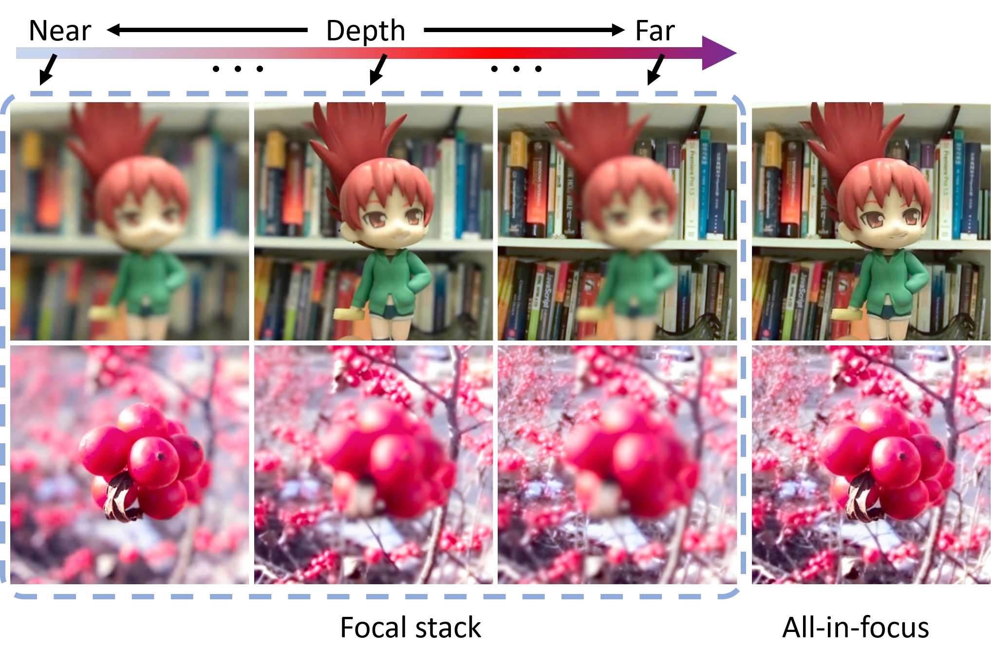
Specifically, a focal stack (left three columns in Fig. 3) contains a series of images focusing on different depths. Such images are generated by processing the raw light field data using digital refocusing techniques [42]. The refocusing principle is demonstrated in Fig. 4, which only shows the case of and dimensions. Suppose a light ray enters the main lens at location . If the imaging plane’s position ( denotes the focal distance of the main lens) is changed to , where , a refocused image can be computed as follows. First, given the 4D light field , the new light field regarding the new imaging plane at can be derived as
| (1) |
Next, after obtaining the new light field , a refocused image on the imaging plane can be synthesized as
| (2) |
One can see that by changing the parameter , a series of refocused images can be generated, composing a focal stack. After the focal stack is obtained, an all-in-focus image can be produced by photo-montage [69]. For example, an all-in-focus image can be generated by putting all the clear pixels together, where the clarity of pixels can be estimated by the associated gradients. Besides, it can also be acquired by computing a weighted average of all the focus slices. More details of the algorithm can be found in [70].
In addition to focal stacks, multi-view images (Fig. 5) can also be derived from light field data. As mentioned before, in the 4D light field representation , encode the angular information of incoming rays. Thus, an image from a certain viewpoint can be generated by sampling at a specific angular direction , and the image can be represented by . By varying , multi-view images can be synthesized. Especially, when the angular direction is equal to that of the central view, namely , the center-view image is achieved. On the other hand, micro-lens images can be generated by sampling the dimensions. Providing a micro-lens location leads to a micro-lens image , which captures multiple perspectives of a scene point. Note that, by varying , different micro-lens images can be obtained, which together compose a micro-lens image array representing complete light field information. A visualization of micro-lens and multi-view images can be found in a recent work [59].

Moreover, depth maps containing scene depth information can also be estimated from a light field. As mentioned, depth information is embedded in the focusness and angular cues, so a depth map can be generated by combining both defocusness and correspondence (angular) cues. For more details on depth estimation from light fields please refer to [38, 39, 40, 41, 43, 44].
II-B Light Field SOD Models and Reviews
In this section, we review and discuss existing models proposed for light field SOD, including ten traditional models that employ hand-crafted features, and seven deep learning-based models. Also, one comparative study and one brief review are revisited. Details of all these works are summarized in Table I.
| Models | Pub. | Year | Training dataset(s) | Testing dataset(s) | Main components | FS | DE | MV | ML | OP | ||||
|---|---|---|---|---|---|---|---|---|---|---|---|---|---|---|
| LFS [5] | CVPR | 2014 | - | LFSD | Focusness measure, location priors, contrast cues, background prior, new dataset (LFSD) | ✓ | ✓ | |||||||
| WSC [50] | CVPR | 2015 | - | LFSD | Weighted sparse coding, saliency/non-saliency dictionary construction | ✓ | ✓ | ✓ | ||||||
| Traditional models | DILF [30] | IJCAI | 2015 | - | LFSD | Depth-induced/Color contrast, background priors by focusness | ✓ | ✓ | ✓ | |||||
| RL [51] | ICASSP | 2016 | - | LFSD | Relative locations, guided filter, micro-lens images | ✓ | ||||||||
| BIF [52] | NPL | 2017 | - | LFSD | Bayesian framework, boundary prior, color/depth-induced contrast | ✓ | ✓ | |||||||
| LFS [6] | TPAMI | 2017 | - | LFSD | An extension of [5] | ✓ | ✓ | |||||||
| MA [53] | TOMM | 2017 | - | LFSD + HFUT-Lytro | Superpixels intra-cue distinctiveness, light-field flow, new dataset (HFUT-Lytro) | ✓ | ✓ | ✓ | ||||||
| SDDF [56] | MTAP | 2018 | - | LFSD | Background priors, gradient operator, color contrast, local binary pattern histograms | ✓ | ||||||||
| SGDC [1] | CVPR | 2018 | - | LFSD | Focusness cues, color and depth contrast | ✓ | ✓ | |||||||
| RDFD [54] | MTAP | 2020 | - | LFSD | Region-based depth feature descriptor, dark channel prior, multi-layer cellular automata | ✓ | ||||||||
| DCA [55] | TIP | 2020 | - | LFSD | Depth-induced cellular automata, object-guided depth | ✓ | ✓ | |||||||
| DLLF [57] | ICCV | 2019 | DUTLF-FS | LFSD + DUTLF-FS | VGG-19, attention subnetwork, ConvLSTM, adversarial examples, new dataset (DUTLF-FS) | ✓ | ||||||||
| Deep learning models | DLSD [45] | IJCAI | 2019 | DUTLF-MV | DUTLF-MV | View synthesis network, multi-view detection/attention, VGG-19, new dataset (DUTLF-MV) | ✓ | ✓ | ||||||
| MoLF [31] | NIPS | 2019 | DUTLF-FS |
|
VGG-19, memory-oriented spatial fusion, memory-oriented feature integration | ✓ | ✓ | |||||||
| ERNet [32] | AAAI | 2020 |
|
|
VGG-19, ResNet-18, multi-focusness recruiting/screening modules, distillation | ✓ | ✓ | |||||||
| LFNet [58] | TIP | 2020 | DUTLF-FS |
|
VGG-19, refine unit, attention block, ConvLSTM | ✓ | ||||||||
| MAC [59] | TIP | 2020 | Lytro Illum |
|
Micro-lens images/image arrays, DeepLab-v2, model angular changes, new dataset (Lytro Illum) | ✓ | ✓ | |||||||
| MTCNet [60] | TCSVT | 2020 | Lytro Illum |
|
Edge detection, depth inference, feature-enhanced salient object generator | ✓ | ||||||||
| Reviews | CS [48] | NEURO | 2015 | - | LFSD | Comparative study between 2D vs. light field saliency | ||||||||
| RGBDS [49] | CVM | 2020 | - | - | In-depth RGB-D SOD survey, brief review of light field SOD |
II-B1 Traditional Models
As summarized in Table I, traditional light field SOD models often extend various hand-crafted features/hypotheses which are widely adopted in conventional saliency detection [4], such as global/local color contrast, background priors, and object location cues, to the case of light field data. Some tailored features like focusness, depth, and light-field flow, are incorporated as well. Besides, these traditional models tend to employ some post-refinement steps, e.g., an optimization framework [30, 51, 53, 1, 55] or CRF [55], to achieve saliency maps with better spatial consistency and more accurate object boundaries. Regarding the data forms leveraged, almost all traditional models work with focal stacks, while depth is incorporated by some of them. Only two traditional models consider using the multi-view [53] and micro-lens data [51]. Further, due to early dataset scarcity, almost all traditional models are evaluated only on the small LFSD dataset constructed by [5]. Despite early progresses made by these traditional models, due to general limitations of hand-crafted features, they can hardly generalize well to challenging and complex scenarios comparing to modern deep learning models. Here below we briefly review the key features of these traditional models without taxonomy, because they adopt overlapped features but quite diverse computational techniques.
LFS [5] was the pioneering and earliest work on light field SOD, where the first dataset was also proposed. LFS first incorporated the focusness measure with location priors to determine the background and foreground slices. Then, in the all-focus44 4 In this paper, “all-focus” and “all-in-focus” are used interchangeably. Their meanings are the same. image, it computed the background prior and contrast cues to detect saliency candidates. Finally, a saliency map was generated by incorporating the saliency candidates in the all-focus image with those in the foreground slices, where objectness cues were used to weight the candidates. An extension of this work was published in [6].
WSC [50] was proposed as a unified framework for 2D, 3D and light field SOD problems, which can handle heterogeneous data. Based on the weighted sparse coding framework, the authors first used a non-saliency dictionary to reconstruct a reference image, where patches with high reconstruction error were selected as the saliency dictionary. This saliency dictionary was later refined by iteratively running the weighted sparse framework to achieve the final saliency map. For the light field data, features used for dictionary construction were derived from the all-focus RGB image, depth map, and also focal stacks.

DILF [30] computed the depth-induced contrast saliency and color contrast saliency from the all-focus image and depth image, which were then used to generate a contrast saliency map. It also computed the background priors based on the focusness measure embedded in the focal stacks and used them as weights to eliminate background distraction and enhance saliency estimation.
RL [51] proposed to estimate the relative locations of scene points using a filtering process. Such relative locations, which can be treated as conveying scene depth information, were then incorporated with the robust background detection and saliency optimization framework proposed in [71] to achieve enhanced saliency detection.
BIF [52] used the Bayesian framework to fuse multiple features extracted from RGB images, depth maps and focal stacks. Inspired by image SOD methods, this model utilized a boundary connectivity prior, background likelihood scores and color contrast to generate background probability maps, foreground slices, color-based saliency maps and depth-induced contrast maps, which are fused by a two-stage Bayesian scheme.
MA [53] measured the saliency of a superpixel by computing the intra-cue distinctiveness between two superpixels, where features considered include color, depth, and flow inherited from different focal planes and multiple viewpoints. The light-field flow was first employed in this method, estimated from focal stacks and multi-view sequences, to capture depth discontinuities/contrast. The saliency measure was later enhanced using a location prior and a random-search-based weighting strategy. In addition, the authors proposed a new light field SOD dataset, which was the largest at that time.
SDDF [56] made use of depth information embedded in focal stacks to conduct accurate saliency detection. A background measurement was first obtained by applying a gradient operator to focal stack images, and the focal slice with the highest measurement was chosen as the background layer. A coarse prediction was generated by separating the background and foreground in the all-focus image using the derived background regions, and the final saliency map was calculated globally via both color and texture (local binary pattern histograms) contrast based on the coarse saliency map.
SGDC [1] presented an approach named contrast-enhanced saliency detection for optimizing the multi-layer light field display. It first computed a superpixel-level focusness map for each refocused image and then chose the refocused image with the highest background likelihood score to derive background cues. Such focusness background cues were later incorporated with color and depth contrast saliency. The final results were optimized by the optimization framework proposed in [71].
RDFD [54] addressed the light field SOD problem via a multiple cue integration framework. A region-based depth feature descriptor (RDFD) defined over the focal stack was proposed, which was based on the observation that dark channel priors [72] can be used to estimate the degree of defocusing/blurriness. The RDFD was generated by integrating the degrees of defocusing over all focal stack images, alleviating the limitation of requiring accurate depth maps. RDFD features were used to compute a region-based depth contrast map and a 3D spatial distribution prior. These cues were merged into a single map using a multi-layer cellular automata (MCA).
DCA [55] proposed a depth-induced cellular automata (DCA) for light field SOD. Firstly, it used the focusness and depth cue to calculate the object-guided depth map and select background seeds. Based on the seeds, a contrast saliency map was computed and multiplied with the object-guided depth map to achieve a depth-induced saliency map, which was subsequently optimized by DCA. Finally, the optimized map was combined with the depth-induced saliency map. A Bayesian fusion strategy and CRF were employed to refine the prediction.

II-B2 Deep Learning-based Models
Due to the powerful learning ability of deep neural networks, deep learning-based models can achieve superior accuracy and performance [57] over traditional light field SOD models. Another advantage of deep models comparing to the latter is that they can directly learn from a large amount of data without hand-crafted feature engineering. Therefore, as overviewed in Table I, one can see that the scarcity of datasets has been somewhat alleviated in the deep learning era, as three new datasets have been introduced to better train deep neural networks. Still, most deep models take a focal stack as network input. Due to the multi-variable property of focal stacks, modules such as attention mechanisms [57, 45, 31, 58, 32] and ConvLSTMs [57, 31, 58, 32] are preferred. We argue that there may be different ways of taxonomy for deep models. A straightforward way is to categorize according to what kind of light field data is utilized, as indicated in Table I. While there are four models, namely DLLF [57], MoLF [31], ERNet [32], LFNet [58] resorting to focal stacks, DLSD [45] and MTCNet [60] utilize multi-view images, and MAC [59] explores micro-lens images. Different input data forms often lead to different network designs. Note that for DLSD [45], multi-view images processed are indeed rendered from an input single-view image, so this method can be applied to cases no matter multi-view images are available or not.
However, since using deep learning-based techniques for light field SOD is the leading trend, in this paper, we further propose to divide existing deep models into five categories according to their architectures, including late-fusion scheme, middle-fusion scheme, knowledge distillation-based scheme, reconstruction-based scheme, and single-stream scheme, as illustrated in Fig. 6. Their descriptions and associated models are briefly introduced as follows.
Late-fusion. Late-fusion models (Fig. 6 (a), DLLF [57], MTCNet [60]) aim at obtaining individual predictions from the input focal stack/multi-view images and all-focus/center-view image, and then simply fuses the results. Note that late fusion is a classical strategy also widely adopted in previous multi-modal detection works (e.g., RGB-D SOD [49], RGB-D semantic segmentation [73, 34]) due to its simplicity and easy implementation. However, the fusion process is restrained to the last step with relatively simple integrative computation.
DLLF [57] adopted a two-stream fusion framework that explored focal stacks and all-in-focus images separately. In the focal stack stream, DLLF first extracted features from cascaded focal slices through a fully convolutional network. Diverse features from different slices were then integrated by a recurrent attention network, which employed an attention subnetwork and ConvLSTM [74] to adaptively incorporate weighted features of slices and exploit their spatial relevance. The generated map was lately combined with another saliency map derived from the all-in-focus image. In addition, to address the limitation of data for training deep networks, a new large dataset was introduced.
MTCNet [60] proposed a two-stream multi-task collaborative network, consisting of a saliency-aware feature aggregation module (SAFA) and multi-view inspired depth saliency feature extraction (MVI-DSF) module, to extract representative saliency features with the aid of the correlation mechanisms across edge detection, depth inference and salient object detection. SAFA simultaneously extracted focal-plane, edge and heuristic saliency features from a center-view image, while MVI-DSF inferred depth saliency features from a set of multi-view images. Finally, MTCNet combined the extracted features using a feature-enhanced operation to obtain the final saliency map.
Middle-fusion. The middle-fusion strategy (Fig. 6 (b), MoLF [31], LFNet [58]) extracts features from the focal stack and all-focus image in a two-stream manner. Fusion across intermediate features is then done by an elaborate and complex decoder. Comparing to the late-fusion strategy in Fig. 6 (a), the main differences are that the features fused are usually hierarchical and intermediate, and the decoder is also a relatively deep convolutional network to mine more complex integration rules.
MoLF [31] was featured by a memory-oriented decoder that consists of spatial fusion module (Mo-SFM) and feature integration module (Mo-FIM), in order to resemble the memory mechanism of how humans fuse information. Mo-FSM utilized an attention mechanism to learn the importance of different feature maps and a ConvLSTM [74] to gradually refine spatial information. In Mo-FIM, a scene context integration module (SCIM) and ConvLSTM were employed to learn channel attention maps and summarize spatial information.
LFNet [58] proposed a two-stream fusion network to refine complementary information and integrate focusness and blurriness, which change gradually in focal slices. Features extracted from the all-focus image and focal stack are fed to a light field refinement module (LFRM) and integration module (LFIM) to generate a final saliency map. In LFRM, features extracted from a single slice were fed to a refinement unit to learn the residuals. In LFIM, an attention block was used to adaptively weight and aggregate slice features.
Knowledge distillation-based. Different from the aforementioned late-fusion/middle-fusion schemes that investigate how to fuse focal stack and all-focus features, the knowledge distillation-based scheme (Fig. 6 (c), ERNet [32]) attempts to transfer focusness knowledge of a teacher network that handles focal stacks, to a student network that processes all-focus images. It uses both the features and prediction from the focal stack stream to supervise those features and prediction obtained from the all-focus stream, effectively boosting the performance of the latter. In this sense, the student network is actually an RGB SOD network augmented by extra light field knowledge during training.
ERNet [32] consisted of two-stream teacher-student networks based on knowledge distillation. The teacher network used a multi-focusness recruiting module (MFRM) and a multi-focusness screening module (MFSM) to recruit and distil knowledge from focal slices, while the student network took a single RGB image as input for computational efficiency and was enforced to hallucinate multi-focusness features as well as the prediction from the teacher network.
Reconstruction-based. Comparing to the above three categories, the reconstruction-based scheme (Fig. 6 (d), DLSD [45]) focuses on a different aspect as well, namely reconstructing light field data/information from a single input image. This is indeed another interesting topic as light field has various data forms (Section II-A2). With the assistance of the reconstructed light field, an encoder-decoder architecture with middle-/late-fusion strategy can then be employed to complete light field SOD. In other words, this scheme is similar to the role of student network in the knowledge distillation-based scheme, namely that it is essentially an RGB SOD network augmented by extra light field knowledge during training (in this case, learns to reconstruct light field data).
DLSD [45] treated light field SOD as two sub-problems: light field synthesis from a single-view image and light-field-driven SOD. This model first employed a light field synthesis network, which estimated depth maps along the horizontal and vertical directions with two independent convolutional networks. According to the depth maps, the single-view image was warped into horizontal and vertical viewpoints of the light field. A light-field-driven SOD network, consisting of a multi-view saliency detection subnetwork and multi-view attention module, was designed for saliency prediction. Specifically, this model inferred a saliency map from a 2D single-view image, but utilized the light field (the multi-view data) as a middle bridge. To train the model, a new dataset containing multi-view images and pixel-wise ground-truth of central view was introduced.
| Dataset | Scale | Spatial resolution | Angular resolution | MOP | FS | MV | DE | ML | GT | Raw | Device |
|---|---|---|---|---|---|---|---|---|---|---|---|
| LFSD [5] | 100 (No offical split) | 360 360 | - | 0.04 | ✓ | ✓ | ✓ | ✓ | Lytro | ||
| HFUT-Lytro [53] | 255 (No offical split) | 328 328 | 7 7 | 0.29 | ✓ | ✓ | ✓ | ✓ | Lytro | ||
| DUTLF-FS [57] | 1462 (1000 train, 462 test) | 600 400 | - | 0.05 | ✓ | ✓ | ✓ | Lytro Illum | |||
| DUTLF-MV [45] | 1580 (1100 train, 480 test) | 590 400 | 7 7 | 0.04 | ✓ | ✓ | Lytro Illum | ||||
| Lytro Illum [59] | 640 (No offical split) | 540 375 | 9 9 | 0.15 | ✓ | ✓ | ✓ | Lytro Illum |
Single-stream. Lastly, the single-stream scheme (Fig. 6 (e), MAC [59]) is inspired by the fact that light field can be formulated in a single image representation, namely the micro-lens image array [59]. Therefore, unlike Fig. 6 (a) and (b), this scheme processes the micro-lens image array directly using a single bottom-up stream, without explicit feature fusion.
MAC [59] was an end-to-end deep convolutional network for light field SOD with micro-lens image arrays as input. Firstly, it adopted a MAC (Model Angular Changes) block tailored to model angular changes in individual local micro-lens image and then fed the extracted features to a modified DeepLab-v2 network [75], capturing multiscale information and long-range spatial dependencies. Together with the model, a new Lytro Illum dataset containing high-quality micro-lens image arrays was proposed.
II-B3 Other Review Works
CS [48]. This paper provided a comparative study between light field saliency and 2D saliency, showing the advantage of conducting the SOD task on light field data over single 2D images. It compared the classical model LFS [5] with eight 2D saliency models on the LFSD dataset [5]. Five evaluation metrics were used in the paper to show that the light field saliency model achieved better and more robust performance than conventional 2D models.
RGBDS [49]. This paper conducted an in-depth and comprehensive survey on RGB-D salient object detection. It reviewed existing RGB-D SOD models from various perspectives, as well as the related benchmark datasets in detail. Considering the fact that light fields can also provide depth maps, the authors also briefly reviewed the light field SOD models and datasets. However, because the main focus of this paper was on RGB-D SOD, very few contents are given to review light field SOD, and no associated benchmarking was conducted.
II-C Light Field SOD Datasets
At present, there are five datasets introduced for the light field SOD task, including LFSD [5], HFUT-Lytro [53], DUTLF-FS [57], DUTLF-MV [45], and Lytro Illum [59]. Beyond Table I, we summarize details of these datasets in Table II and show some samples from four datasets (i.e., LFSD, HFUT-Lytro, Lytro Illum, and DUTLF-FS) in Fig. 7. A brief introduction is given as follows:

LFSD55 5 https://sites.duke.edu/nianyi/publication/saliency-detection-on-light-field/ [5] was the first light field dataset collected for SOD, and contains 60 indoor and 40 outdoor scenes. This dataset was captured by a Lytro camera and provides a focal stack, all-in-focus image, depth map and the corresponding ground-truth for each light field. The image spatial resolution is 360360. Besides, raw light field data is also available in LFSD. Note that most images in this dataset contain one single center-placed object with a relatively simple background.
HFUT-Lytro66 6 https://github.com/pencilzhang/MAC-light-field-saliency-net [53] contains 255 light fields for both indoor and outdoor scenes. Each light field contains a focal stack whose slice numbers vary from 1 to 12. The angular resolution is 7 7 and the spatial resolution is 328 328. Notably, focal stacks, all-in-focus images, multi-view images and coarse depth maps are all provided in this dataset. Several challenges regarding SOD, e.g., occlusions, cluttered background and appearance changes, are present in HFUT-Lytro.
DUTLF-FS77 7 https://github.com/OIPLab-DUT/ICCV2019_Deeplightfield_Saliency [57] is one of the largest light field SOD datasets to date, containing 1,462 light fields in total. It was acquired by a Lytro Illum camera in both indoor and outdoor scenes. The entire dataset is officially divided into 1,000 training samples and 462 testing samples. All-focus images, focal stacks and the corresponding ground-truth are provided for different light fields. The slice number of a focal stack ranges from 2 to 12, and the image spatial resolution is 600 400. It is worth noting that DUTLF-FS covers various challenges, including different types of objects, low appearance contrast between salient objects and their background, and varied object locations.
DUTLF-MV88 8 https://github.com/OIPLab-DUT/IJCAI2019-Deep-Light-Field-Driven-Saliency-Detection-from-A-Single-View [45] is another large-scale light field dataset for SOD, which was generated from the same database as DUTLF-FS (with 1,081 identical scenes). In contrast to other datasets, this dataset was proposed to better exploit the angular cues. Therefore, only multi-view images with respect to horizontal and vertical viewpoints are available, together with the ground-truth of the center view image. DUTLF-MV contains 1,580 light fields in total, and is officially divided into training and test sets with 1,100 and 480 samples, respectively. The spatial resolution of each image is 400 590 and the angular resolution is 7 7.
Lytro Illum6 [59] contains 640 high-quality light fields captured by a Lytro Illum camera. The images in this dataset vary significantly in object size, texture, background clutter and illumination. Lytro Illum provides center-view images, micro-lens image arrays, raw light field data, as well as the corresponding ground-truths of the center-view images. The resolution of micro-lens image arrays is 4860 3375, while center-view images and ground-truths have a 540 375 spatial resolution. The angular resolution can be inferred as 9 9.


Dataset Analysis. From the summarization in Table II, we can observe two issues existed in current datasets, namely scale limitation and non-unified data forms. Compared to the large datasets constructed for the conventional SOD task, such as DUT-OMRON (5,168 images) [76], MSRA10K (10,000 images) [2] and DUTS (15,572 images) [77], the existing light field SOD datasets are still small, making it somewhat difficult to evaluate data-driven models and train deep networks. Besides, their data forms are not always consistent. For example, Lytro Illum does not provide focal stacks, while DUTLF-FS/DUTLF-MV only provide focal stacks/multi-view images without offering the raw data. This makes comprehensive benchmarking very difficult, because a model using focal stacks as input cannot run on DUTLF-MV and Lytro Illum. We will show how we alleviate this problem in Section III-B, and discuss the underlying future directions in Section IV.
To better understand the above-mentioned datasets, we have conducted statistical analyses, including size ratios of salient objects, distributions of normalized object distances from image centers, numbers of focal slices and numbers of objects. The quantitative results are shown in Fig. 8 and Fig. 9. From Fig. 8 (a), we can see that most objects from these datasets have size ratios lower than 0.6. HFUT-Lytro and Lytro Illum have relatively small objects, while LFSD has objects that are relatively large in size. Fig. 8 (b) and Fig. 9 clearly show the spatial distributions of objects. From Fig. 9, we can see that all five datasets present strong center bias, and Fig. 8 (b) reveals that objects from Lytro Illum are generally the closest to the image centers (also indicated by Fig. 9).
In addition, the statistics on focal slice numbers are given in Fig. 8 (c). Note that only three datasets, namely LFSD, HFUT-Lytro, and DUTLF-FS, provide focal slices. The numbers of slices vary from 1 to 12 and there are notable differences between different datasets. The slice numbers corresponding to the distribution peaks on LFSD, HFUT-Lytro and DUTLF-FS are 12, 3, and 6, respectively. All three datasets have various slices numbers, indicating that a light field SOD model using focal stacks should be able to handle various numbers of input slices. Lastly, from Fig. 8 (d), we can see that most images from these datasets have a single object. Also, HFUT-Lytro and Lytro Illum have some images with multiple objects (with higher “MOP” in Table II), which could be useful for validating models on detecting multiple objects.
III Model Evaluation and Benchmark
In this section, we first review five popular evaluation metrics, and then provide a pipeline for achieving dataset unification. Moreover, we carry out a benchmarking evaluation and provide an experimental result analysis.
III-A Evaluation Metrics
In our benchmarking of light field SOD models, we employ nine metrics, which are universally agreed upon and are described as follows:
Precision-recall (PR) [78, 3, 2] curve is defined as:
| (3) |
where is a binary mask obtained by thresholding the saliency map with threshold , and is the total area of the mask. denotes the ground-truth. A comprehensive precision-recall curve is obtained by changing from 0 to 255.
F-measure [78, 3, 2] is defined as the harmonic-mean of precision and recall:
| (4) |
where is the weight between and , and is often set to 0.3 to emphasize more on precision. Since different F-measure scores can be obtained according to different precision-recall pairs, in this paper, we report the maximum F-measure () and mean F-measure () computed from the PR curve. Besides, we also report the adaptive F-measure () [78], whose threshold is computed as the twice of the mean of a saliency map.
Mean Absolute Error () [79] is defined as:
| (5) |
where and denote the values at the -th pixel in the saliency map and ground-truth map. is the total number of pixels in the both map.
S-measure [80, 81] was proposed to measure the spatial structure similarities between the saliency map and ground-truth. It is defined as:
| (6) |
where and denote the object-aware and region-aware structural similarity, respectively, and balances and . In this paper, we set , as recommended in [80].
E-measure [82] is a recently proposed metric which considers both the local and global similarity between the prediction and ground-truth. It is defined as:
| (7) |
where denotes the enhanced alignment matrix [82]. and are the width and height of the ground-truth map, while are pixel indexes. Since also performs a comparison between two binary maps, we treat it similarly to the F-measure, thresholding a saliency map with all possible values and reporting the maximum and mean , denoted as and . Besides, adaptive , namely , is computed similarly to the adaptive F-measure mentioned above, where the thresholds are two times the mean saliency values [78].
Note that, higher PR curves, , and , and lower indicate better performance.
| Datasets | FS | MV | DE | ML | Raw |
|---|---|---|---|---|---|
| LFSD [5] | ✓ | ⚪ | ✓ | ⚪ | ✓ |
| HFUT-Lytro [53] | ✓ | ✓ | ✓ | ⚪ | |
| DUTLF-FS [57] | ✓ | ✓ | |||
| DUTLF-MV [45] | ✓ | ||||
| Lytro Illum [59] | ⚪ | ⚪ | ⚪ | ✓ | ✓ |
III-B Dataset Unification
As shown in Section II-Cand Table II, existing light field SOD datasets face the limitation of having non-unified data forms. This makes comprehensive benchmarking difficult. Since, due to the lack of specific data, some models cannot be correctly evaluated on certain datasets. To alleviate this issue, we generate supplemental data for existing datasets, making them complete and unified. The completed data forms are illustrated in Table III, marked by “⚪”. Furthermore, we will release this data on our project site: https://github.com/kerenfu/LFSOD-Survey to facilitate future research in this field.

Generally, we can synthesize various data forms using the raw light field data, provided by two datasets, i.e., LFSD and Lytro Illum. For Lytro Illum, we generate focal stacks (including all-in-focus images) and depth maps using the Lytro Desktop software. Regarding focal stack generation, we estimate the approximate focus range for each image scene, and then sample the focal slices within the focus range by an equal step. All-blurred or duplicated slices are removed. The final number of generated focal slices for Lytro Illum ranges from 2 to 16 for each scene, and about 74% of scenes have more than 6 slices. Fig. 10 shows an example of the generated focal stack. As mentioned in Section II-A2, multi-view images and micro-lens image arrays are generated by sampling the light field data in angular and spatial resolution, respectively. Thus, these two data forms can be transformed between each other. In this way, we generate multi-view images for Lytro Illum from its micro-lens image arrays. We can also synthesize micro-lens image arrays for HFUT-Lytro through the reverse operation. However, we cannot synthesize micro-lens image arrays for DUTLF-MV since the authors have only released the multi-view images in the vertical/horizontal direction. By using the raw data, we complement multi-view images and micro-lens image arrays for LFSD (Fig. 11). This complete data makes more comprehensive model evaluation possible. For example, models based on focal stacks, such as MoLF and ERNet, can now run and test on Lytro Illum. Note that for the remaining DUTLF-FS and DUTLF-MV, supplementing more data is possible in the future if the authors release the raw/more data. If this has been done, DUTLF-FS/DUTLF-MV has the potential to be the standard training dataset for future models thanks to its large scale.
| Traditional | Deep learning-based | ||||||||||||||||||||||||||||||||||||||||||||||||||||||
|---|---|---|---|---|---|---|---|---|---|---|---|---|---|---|---|---|---|---|---|---|---|---|---|---|---|---|---|---|---|---|---|---|---|---|---|---|---|---|---|---|---|---|---|---|---|---|---|---|---|---|---|---|---|---|---|
| Metric |
|
|
|
|
|
|
|
|
|
|
|
|
|
|
|
|
|
| |||||||||||||||||||||||||||||||||||||
| LFSD[5] | 0.681 | 0.702 | 0.811 | 0.786 | 0.786 | 0.825 | 0.831 | 0.820 | 0.789 | 0.864 | 0.862 | 0.859 | 0.858 | 0.825 | 0.837 | 0.850 | 0.846 | 0.858 | |||||||||||||||||||||||||||||||||||||
| 0.744 | 0.743 | 0.811 | 0.802 | 0.784 | 0.824 | 0.842 | 0.824 | 0.788 | 0.858 | 0.867 | 0.868 | 0.859 | 0.812 | 0.835 | 0.858 | 0.837 | 0.866 | ||||||||||||||||||||||||||||||||||||||
| 0.513 | 0.722 | 0.719 | 0.735 | 0.758 | 0.800 | 0.829 | 0.794 | 0.753 | 0.842 | 0.848 | 0.862 | 0.848 | 0.797 | 0.806 | 0.850 | 0.818 | 0.856 | ||||||||||||||||||||||||||||||||||||||
| 0.735 | 0.743 | 0.795 | 0.802 | 0.779 | 0.810 | 0.831 | 0.806 | 0.793 | 0.840 | 0.827 | 0.862 | 0.838 | 0.788 | 0.803 | 0.857 | 0.818 | 0.852 | ||||||||||||||||||||||||||||||||||||||
| 0.809 | 0.789 | 0.861 | 0.851 | 0.859 | 0.880 | 0.884 | 0.885 | 0.836 | 0.900 | 0.902 | 0.901 | 0.898 | 0.863 | 0.873 | 0.896 | 0.880 | 0.902 | ||||||||||||||||||||||||||||||||||||||
| 0.567 | 0.753 | 0.764 | 0.758 | 0.819 | 0.864 | 0.879 | 0.867 | 0.790 | 0.883 | 0.894 | 0.890 | 0.893 | 0.850 | 0.855 | 0.881 | 0.869 | 0.899 | ||||||||||||||||||||||||||||||||||||||
| 0.773 | 0.788 | 0.846 | 0.834 | 0.852 | 0.879 | 0.882 | 0.882 | 0.839 | 0.889 | 0.882 | 0.896 | 0.890 | 0.853 | 0.863 | 0.890 | 0.872 | 0.897 | ||||||||||||||||||||||||||||||||||||||
| 0.205 | 0.150 | 0.136 | 0.136 | 0.117 | 0.092 | 0.083 | 0.092 | 0.118 | 0.072 | 0.070 | 0.067 | 0.072 | 0.095 | 0.094 | 0.073 | 0.086 | 0.068 | ||||||||||||||||||||||||||||||||||||||
| HFUT-Lytro[53] | 0.565 | 0.613 | 0.672 | 0.619 | 0.711 | 0.742 | 0.778 | 0.736 | 0.731 | 0.751 | 0.789 | 0.725 | 0.748 | 0.749 | 0.729 | 0.723 | 0.763 | 0.772 | |||||||||||||||||||||||||||||||||||||
| 0.427 | 0.508 | 0.601 | 0.533 | 0.624 | 0.662 | 0.722 | 0.657 | 0.667 | 0.676 | 0.727 | 0.647 | 0.677 | 0.671 | 0.650 | 0.626 | 0.690 | 0.729 | ||||||||||||||||||||||||||||||||||||||
| 0.323 | 0.493 | 0.513 | 0.469 | 0.594 | 0.639 | 0.709 | 0.628 | 0.620 | 0.654 | 0.707 | 0.639 | 0.672 | 0.651 | 0.623 | 0.617 | 0.669 | 0.706 | ||||||||||||||||||||||||||||||||||||||
| 0.427 | 0.485 | 0.530 | 0.518 | 0.592 | 0.627 | 0.706 | 0.615 | 0.638 | 0.654 | 0.677 | 0.636 | 0.675 | 0.647 | 0.588 | 0.636 | 0.653 | 0.689 | ||||||||||||||||||||||||||||||||||||||
| 0.637 | 0.695 | 0.748 | 0.712 | 0.784 | 0.812 | 0.841 | 0.799 | 0.797 | 0.801 | 0.844 | 0.778 | 0.804 | 0.797 | 0.777 | 0.784 | 0.801 | 0.833 | ||||||||||||||||||||||||||||||||||||||
| 0.524 | 0.684 | 0.657 | 0.623 | 0.749 | 0.790 | 0.832 | 0.777 | 0.733 | 0.765 | 0.825 | 0.763 | 0.793 | 0.773 | 0.756 | 0.746 | 0.788 | 0.819 | ||||||||||||||||||||||||||||||||||||||
| 0.666 | 0.680 | 0.693 | 0.691 | 0.755 | 0.785 | 0.831 | 0.770 | 0.772 | 0.804 | 0.811 | 0.781 | 0.810 | 0.789 | 0.744 | 0.779 | 0.789 | 0.810 | ||||||||||||||||||||||||||||||||||||||
| 0.221 | 0.154 | 0.150 | 0.223 | 0.111 | 0.094 | 0.082 | 0.103 | 0.107 | 0.089 | 0.075 | 0.100 | 0.090 | 0.091 | 0.112 | 0.097 | 0.095 | 0.084 | ||||||||||||||||||||||||||||||||||||||
| Lytro Illum[59] | 0.619 | 0.709 | 0.756 | 0.738 | 0.788 | 0.834 | 0.843 | N/T | N/T | 0.879 | 0.890 | 0.872 | 0.865 | 0.869 | 0.853 | 0.881 | 0.873 | 0.883 | |||||||||||||||||||||||||||||||||||||
| 0.545 | 0.662 | 0.697 | 0.696 | 0.746 | 0.820 | 0.827 | N/T | N/T | 0.850 | 0.878 | 0.850 | 0.843 | 0.843 | 0.823 | 0.857 | 0.855 | 0.875 | ||||||||||||||||||||||||||||||||||||||
| 0.385 | 0.646 | 0.604 | 0.624 | 0.713 | 0.766 | 0.800 | N/T | N/T | 0.829 | 0.848 | 0.836 | 0.827 | 0.818 | 0.788 | 0.839 | 0.823 | 0.848 | ||||||||||||||||||||||||||||||||||||||
| 0.547 | 0.639 | 0.659 | 0.679 | 0.720 | 0.747 | 0.796 | N/T | N/T | 0.828 | 0.830 | 0.835 | 0.824 | 0.813 | 0.778 | 0.835 | 0.823 | 0.842 | ||||||||||||||||||||||||||||||||||||||
| 0.721 | 0.804 | 0.830 | 0.816 | 0.871 | 0.908 | 0.911 | N/T | N/T | 0.913 | 0.931 | 0.913 | 0.910 | 0.909 | 0.895 | 0.914 | 0.913 | 0.929 | ||||||||||||||||||||||||||||||||||||||
| 0.546 | 0.791 | 0.726 | 0.738 | 0.830 | 0.882 | 0.900 | N/T | N/T | 0.900 | 0.919 | 0.907 | 0.904 | 0.894 | 0.873 | 0.907 | 0.898 | 0.919 | ||||||||||||||||||||||||||||||||||||||
| 0.771 | 0.797 | 0.812 | 0.815 | 0.855 | 0.876 | 0.900 | N/T | N/T | 0.912 | 0.914 | 0.917 | 0.907 | 0.907 | 0.878 | 0.915 | 0.904 | 0.917 | ||||||||||||||||||||||||||||||||||||||
| 0.197 | 0.115 | 0.132 | 0.142 | 0.086 | 0.065 | 0.056 | N/T | N/T | 0.047 | 0.042 | 0.044 | 0.048 | 0.050 | 0.063 | 0.045 | 0.051 | 0.041 | ||||||||||||||||||||||||||||||||||||||
| DUTLF-FS [57] | 0.585 | 0.656 | 0.725 | 0.658 | N/T | 0.887 | 0.899 | 0.878 | 0.804 | 0.894 | 0.905 | 0.908 | 0.870 | 0.852 | 0.845 | 0.906 | 0.868 | 0.905 | |||||||||||||||||||||||||||||||||||||
| 0.533 | 0.617 | 0.671 | 0.599 | N/T | 0.903 | 0.908 | 0.891 | 0.792 | 0.884 | 0.908 | 0.915 | 0.864 | 0.840 | 0.829 | 0.906 | 0.857 | 0.915 | ||||||||||||||||||||||||||||||||||||||
| 0.358 | 0.607 | 0.582 | 0.538 | N/T | 0.855 | 0.891 | 0.843 | 0.746 | 0.867 | 0.885 | 0.907 | 0.854 | 0.820 | 0.806 | 0.893 | 0.841 | 0.899 | ||||||||||||||||||||||||||||||||||||||
| 0.525 | 0.617 | 0.663 | 0.599 | N/T | 0.843 | 0.885 | 0.831 | 0.790 | 0.872 | 0.874 | 0.903 | 0.850 | 0.826 | 0.791 | 0.887 | 0.835 | 0.893 | ||||||||||||||||||||||||||||||||||||||
| 0.711 | 0.788 | 0.802 | 0.774 | N/T | 0.939 | 0.949 | 0.930 | 0.863 | 0.923 | 0.943 | 0.946 | 0.909 | 0.891 | 0.883 | 0.936 | 0.898 | 0.943 | ||||||||||||||||||||||||||||||||||||||
| 0.511 | 0.759 | 0.695 | 0.686 | N/T | 0.921 | 0.943 | 0.912 | 0.806 | 0.908 | 0.932 | 0.939 | 0.904 | 0.874 | 0.866 | 0.928 | 0.889 | 0.938 | ||||||||||||||||||||||||||||||||||||||
| 0.742 | 0.787 | 0.813 | 0.782 | N/T | 0.923 | 0.943 | 0.913 | 0.872 | 0.924 | 0.930 | 0.942 | 0.905 | 0.895 | 0.870 | 0.931 | 0.895 | 0.936 | ||||||||||||||||||||||||||||||||||||||
| 0.227 | 0.151 | 0.156 | 0.191 | N/T | 0.051 | 0.039 | 0.054 | 0.102 | 0.054 | 0.043 | 0.036 | 0.059 | 0.069 | 0.079 | 0.041 | 0.065 | 0.039 | ||||||||||||||||||||||||||||||||||||||
| Models |
|
|
|
| ||||||||||||||||
|---|---|---|---|---|---|---|---|---|---|---|---|---|---|---|---|---|---|---|---|---|
| BBS [35] | 0.864 | 0.858 | 0.900 | 0.072 | 0.751 | 0.676 | 0.801 | 0.089 | 0.879 | 0.850 | 0.913 | 0.047 | 0.894 | 0.884 | 0.923 | 0.054 | ||||
| SSF [61] | 0.859 | 0.868 | 0.901 | 0.067 | 0.725 | 0.647 | 0.778 | 0.100 | 0.872 | 0.850 | 0.913 | 0.044 | 0.908 | 0.915 | 0.946 | 0.036 | ||||
| ATSA [36] | 0.858 | 0.866 | 0.902 | 0.068 | 0.772 | 0.729 | 0.833 | 0.084 | 0.883 | 0.875 | 0.929 | 0.041 | 0.905 | 0.915 | 0.943 | 0.039 | ||||
| ERNet [32] | 0.831 | 0.842 | 0.884 | 0.083 | 0.778 | 0.722 | 0.841 | 0.082 | 0.843 | 0.827 | 0.911 | 0.056 | 0.899 | 0.908 | 0.949 | 0.039 | ||||
| S2MA [64] | 0.837 | 0.835 | 0.873 | 0.094 | 0.729 | 0.650 | 0.777 | 0.112 | 0.853 | 0.823 | 0.895 | 0.063 | 0.845 | 0.829 | 0.883 | 0.079 | ||||
| D3Net [63] | 0.825 | 0.812 | 0.863 | 0.095 | 0.749 | 0.671 | 0.797 | 0.091 | 0.869 | 0.843 | 0.909 | 0.050 | 0.852 | 0.840 | 0.891 | 0.069 | ||||
| HDFNet [66] | 0.846 | 0.837 | 0.879 | 0.086 | 0.763 | 0.690 | 0.801 | 0.095 | 0.873 | 0.855 | 0.913 | 0.051 | 0.868 | 0.857 | 0.898 | 0.065 | ||||
| JLDCF [33] | 0.862 | 0.867 | 0.902 | 0.070 | 0.789 | 0.727 | 0.844 | 0.075 | 0.890 | 0.878 | 0.931 | 0.042 | 0.905 | 0.908 | 0.943 | 0.043 | ||||
| BBS* [35] | 0.739 | 0.738 | 0.812 | 0.123 | 0.708 | 0.622 | 0.773 | 0.113 | 0.825 | 0.788 | 0.878 | 0.065 | 0.873 | 0.870 | 0.919 | 0.051 | ||||
| SSF* [61] | 0.790 | 0.793 | 0.861 | 0.097 | 0.687 | 0.612 | 0.781 | 0.112 | 0.833 | 0.799 | 0.886 | 0.059 | 0.881 | 0.889 | 0.930 | 0.050 | ||||
| ATSA* [36] | 0.816 | 0.823 | 0.873 | 0.087 | 0.727 | 0.673 | 0.805 | 0.104 | 0.844 | 0.822 | 0.905 | 0.054 | 0.880 | 0.892 | 0.936 | 0.045 | ||||
| ERNet* [32] | 0.822 | 0.825 | 0.885 | 0.085 | 0.707 | 0.632 | 0.766 | 0.128 | 0.840 | 0.810 | 0.900 | 0.059 | 0.898 | 0.903 | 0.946 | 0.040 | ||||
| S2MA* [64] | 0.827 | 0.829 | 0.873 | 0.086 | 0.672 | 0.572 | 0.735 | 0.133 | 0.839 | 0.802 | 0.885 | 0.060 | 0.894 | 0.893 | 0.934 | 0.046 | ||||
| D3Net* [63] | 0.827 | 0.821 | 0.877 | 0.086 | 0.720 | 0.645 | 0.801 | 0.104 | 0.859 | 0.835 | 0.906 | 0.051 | 0.906 | 0.911 | 0.947 | 0.039 | ||||
| HDFNet* [66] | 0.849 | 0.850 | 0.891 | 0.073 | 0.747 | 0.673 | 0.801 | 0.096 | 0.874 | 0.854 | 0.915 | 0.045 | 0.922 | 0.931 | 0.955 | 0.030 | ||||
| JLDCF* [33] | 0.850 | 0.860 | 0.900 | 0.071 | 0.755 | 0.694 | 0.823 | 0.098 | 0.877 | 0.855 | 0.919 | 0.042 | 0.924 | 0.931 | 0.958 | 0.030 | ||||
III-C Performance Benchmarking and Analysis
To provide an in-depth understanding of the performance of different models, we conduct the first comprehensive benchmarking of nine light field SOD models (i.e., LFS [5], WSC [50], DILF [30], RDFD [54] DLSD [45], MoLF [31], ERNet [32], LFNet [58] MAC [59]) and nine SOTA RGB-D based SOD models99 9 The RGB-D SOD models benchmarked in this paper are selected according to the top models concluded by the recent survey [49] and also the latest open-source models published in ECCV-2020. All depth maps fed to a model are optionally reversed on an entire dataset to fit the best performance of this model. (i.e., BBS [35], JLDCF [33, 34], SSF [61], UCNet [62], D3Net [63], S2MA [64], cmMS [65], HDFNet [66], and ATSA [36]) on four existing light field datasets, including the entire LFSD (100 light fields), HFUT-Lytro (255 light fields), Lytro Illum (640 light fields) datasets and the test set (462 light fields) of DUTLF-FS. Sample images from these datasets are shown in Fig. 7. All the benchmarked models have either publicly available source/executable codes or results provided by the authors (the authors of RDFD [54] and LFNet [58] have sent us the saliency map results). The nine evaluation metrics described previously (i.e., PR, S-measure, max/mean F-measure, max/mean E-measure, adaptive F-measure and E-measure, mean absolute error) are adopted and the results are reported in Table IV. Meanwhile, the PR curves, max F-measure curves and visual comparisons are shown in Fig. 12, Fig. 13, Fig. 14 and Fig. 15, respectively.
It is worth noting that the evaluation is not conducted on the DUTLF-MV dataset [45] since it only provides multi-view images, which are not compatible with the input data forms of most light field SOD models. Further, note that DLSD [45] is not tested on the DUTLF-FS test set because it used quite some test images (36%, according to our verification) from this dataset for training. Also, MAC [59] is not evaluated on Lytro Illum since the authors conducted five-fold cross-validation on this dataset, and therefore it is not directly comparable to other models. Besides, for DUTLF-FS has no available micro-lens image arrays after dataset unification as illustrated in Table III, and the quality of micro-lens image arrays of HFUT-Lytro is fairly low due to the low-quality multi-view images, we follow [59] and instead test MAC on single up-sampled all-in-focus images from these two datasets. In addition, for ERNet [32], we only evaluate the teacher model since its pre-trained student model is not publicly available. Comprehensive analyses are given as follows.


III-C1 Traditional vs. Deep Light Field SOD Models
Compared to the four traditional models shown in Table I, the deep learning-based SOD models clearly have a significant performance boost on all datasets. The best traditional model evaluated, namely DILF, is generally inferior to any deep model. This confirms the power of deep neural networks when applied to this field.
III-C2 Deep Learning-Based Light Field SOD Models
As shown in Table I, MoLF, ERNet and LFNet adopt focal stacks and all-in-focus images as input data forms, while DLSD and MAC handle center-view images and micro-lens image arrays. From Table IV and Fig. 12, it is clear that MoLF, ERNet and LFNet outperform DLSD and MAC. It is also worth noting that MoLF and ERNet achieve the top-2 performance, which is probably because that these two models were trained on the large-scale DUTLF-FS dataset (i.e., 1,000 light fields) with superior network structures. Besides, such results indicate that models based on multi-view or micro-lens images are not as effective as those based on focal stacks. This is probably because that the former are less studied, and the effectiveness of multi-view and micro-lens images is still underexplored. Moreover, the training data may also matter because MAC was trained only on Lytro Illum, which is about half the scale of DUTLF-FS. Among the above five models compared, ERNet attains the top-1 accuracy.
III-C3 Comparison Between Light Field SOD and RGB-D SOD Models
From the quantitative results illustrated in Table IV and Fig. 12, it can be observed that, the latest cutting-edge RGB-D models achieve comparable or even better performance than the light field SOD models. Notably, three RGB-D models, namely JLDCF, SSF, and ATSA, achieve generally better performance than ERNet on most datasets. The underlying reasons may be two-fold. First, RGB-D based SOD has recently drawn extensive research interest and many powerful and elaborate models have been proposed. Inspired by previous research on the RGB SOD problem [83, 28, 84], these models often pursue edge-preserving results from deep neural networks and employ functional modules/architectures, such as boundary supplement unit [61], multi-scale feature aggregation module [36], or UNet-shaped bottom-up/top-down architecture [33, 64, 85]. In contrast, light field SOD has been less explored and the models/architectures evolve slowly. Edge-aware properties have not yet been considered by most existing models. For example, although the attention mechanism and ConvLSTM are adopted in ERNet, no UNet-like top-down refinement is implemented to generate edge-aware saliency maps. As evidenced in Fig. 1 and Fig. 14, the RGB-D SOD models tend to detect more accurate boundaries than existing deep light field SOD models. Second, the other potential reason could be that the RGB-D SOD models are trained on more data. For instance, the universally agreed training set for the RGB-D SOD task contains 2,200 RGB-D scenarios [33], while ERNet [32] was trained only on 1,000 light fields. Thus, the former is more likely to obtain better generalizability.
However, we can still hardly deny the potentials of light fields on boosting the performance of SOD, as recently RGB-D SOD area is much more active (many new competitive models are proposed as mentioned in [49]) than the area of light field SOD. Besides, the performance of ERNet and MoLF is only slightly lower than that of the RGB-D models on the benchmark datasets, which further implies the effectiveness of light fields for SOD [48]. We believe that there is still considerable room for improving light field SOD, because light fields can provide more information than paired RGB and depth images.
Furthermore, in order to eliminate training discrepancy, we conduct experiments by retraining those RGB-D models on a unified training set, namely the training set of DUTLF-FS that contains 1,000 scenarios. We also retrain ERNet to remove its extra HFUT-Lytro training data as shown in Table I. Comparative results are given in Table V, where all the models generally incur certain performance degeneration. Interestingly, after retraining, SSF* can no longer outperform ERNet*, while ATSA* becomes inferior to ERNet* on LFSD and DUTLF-FS. Only JLDCF* and HDFNet* consistently outperform ERNet* with a noticeable margin.
III-C4 Accuracy Across Different Datasets
It is clearly shown in Table IV and Fig. 12 that the models tested perform differently on different datasets. Generally, the models achieve better results on LFSD than on the other three datasets, indicating that LFSD is the easiest dataset for light field SOD, on which the traditional model DILF can even outperform some deep models like DLSD and MAC. In contrast, HFUT-Lytro, Lytro Illum and DUTLF-FS are more challenging. Note that MoLF, ERNet, ATSA behave prominently on DUTLF-FS, probably because they were trained on DUTLF-FS’s training set or training data (Table I). Besides, as mentioned in Section II-C, HFUT-Lytro has many small salient objects, with multiple objects existed per image. The degraded performance of these models on this dataset tells that detecting small/multiple salient objects is still very challenging for existing schemes, no matter for RGB-D based models or light field models. This makes HFUT-Lytro the most difficult among existing light field datasets.
III-C5 Results Visualization
Fig. 14 visualizes some sample results from five light field models, including two traditional methods (i.e., LFS and DILF) and three deep learning-based models (i.e., DLSD, MoLF and ERNet ), and three latest RGB-D based models (i.e., JLDCF, BBS, and ATSA). The first two rows in Fig. 14 show easy cases while the third to fifth rows show cases with complex backgrounds or sophisticated boundaries. The last row gives an example with low color contrast between foreground and background. As can be observed from Fig. 14, RGB-D models perform comparably to or even better than light field models, which confirms the fact that this field is still insufficiently studied. Fig. 15 further shows several scenarios with small and multiple salient objects, where the first three rows show the cases with multiple salient objects and the others show the cases of small objects. According to Fig. 15, both RGB-D based and light field models are more likely to result in erroneous detection, confirming the challenge of handling small/multiple objects for existing techniques.

IV Challenges and Open Directions
This section highlights several future research directions for light field SOD and outlines several open issues.
IV-A Dataset Collection and Unification
As demonstrated in Section II-C, existing light field datasets are limited in scale and have non-unified data forms, making it somewhat difficult to evaluate different models and generalize deep networks. This non-unified issue is particularly severe for light field SOD because of its diverse data representations and high dependency on special acquisition hardware, differing it from other SOD tasks (e.g., RGB-D SOD [33, 61, 36], video SOD [86, 87]) in the saliency community. Therefore, developing large-scale and unified datasets is essential for future research. We urge researchers to take this issue into consideration when constructing new datasets. Moreover, collecting complete data forms, including raw data, focal stacks, multi-view images, depth maps, and micro-lens image arrays, would definitely facilitate and advance research on this topic. However, we also note there is a challenge in data storage and transmission, since raw light field data is quite large in size (e.g., the 640 light fields of Lytro Illum occupy 32.8 Gigabytes), not to mention a large-scale dataset. The scale of the dataset makes it a bit difficult to spread. In this case, it will still be great if a subset of any data form is available for the public.

IV-B Further Investigations in Light Field SOD
As discussed, there are currently fewer studies regarding SOD on light fields compared to other tasks in the saliency community. Thus, this field is still less active and under-explored. Besides, from the benchmarking results in Section III-C, it can be observed that the SOTA performance is still far from satisfactory, especially on the HFUT-Lytro dataset. There is considerable room for further improvement of light field SOD algorithm/model. In addition, we can notice that only seven deep learning-based models appeared between 2019 and 2020. We attribute such a scarcity of light field SOD research to the aforementioned data problems, as well as the lack of a complete survey of existing methods and datasets on this topic.
IV-C Multi-view Images and Micro-lens Image Arrays
Most existing models work with focal stacks and depth maps, as summarized in Table I, while multi-view images and micro-lens image arrays are two other types of light field data representations that are rarely considered (only five related models). The benchmarking results in Section III-C show that the related models do not perform as well as models utilizing other data forms, so the use of these two data forms has not yet been fully explored. Thus, it is expected to develop more light field SOD models in the future for exploring the effectiveness of multi-view images and micro-lens image arrays. Another potential reason could be that, these two data forms themselves may be less information-representative than focal stacks and depth maps, namely scene depth information is more implicitly conveyed. This may make it difficult to find effective mappings and mine underlying rules using deep neural networks, especially when the training data is sparse. In addition, it is an interesting work to compare the effectiveness and redundancy of saliency detection using different data forms.
IV-D Incorporating High-Quality Depth Estimation
It has been proven that accurate depth maps are conducive to discovering salient objects from complex backgrounds. Unfortunately, the quality of depth maps varies greatly in several existing datasets, since depth estimation from light fields is a challenging task [38, 39, 40, 41, 43, 44]. The challenge stems from the fact that although the light fields can be used to synthesize images focused at any depth through digital refocusing technology, the depth distribution of each scene point is unknown. Besides, it is necessary to determine whether the image area is in focus, which itself is an unresolved issue [88, 89]. Imperfect depth maps often result in negative effects on the detection accuracy of models using depth maps. Therefore, incorporating high-quality depth estimation algorithms from light field is for sure beneficial for boosting performance.
IV-E Edge-Aware Light Field SOD
Accurate object boundaries are essential for high-quality saliency maps, as SOD is a pixel-wise segmentation task [3]. In the RGB SOD field, edge-aware SOD models are drawing increasing research attention [83, 28, 84]. Currently, as shown in our experimental results, existing deep light field SOD models rarely consider this issue, resulting in saliency maps with coarse boundaries/edges. Thus, edge-aware light field SOD could be a future research direction.
IV-F Development of Acquisition Technology and Hardware
As mentioned before, the first generation light field camera, named Lytro, was invented in 2011, while its successor, called Lytro Illum, was introduced in 2014. The latter is more powerful but has a much large size than the former, and is also much more expensive. However, in general, the development of light field acquisition technology and hardware has been slower than that of IT fields such as computers and mobile phones. Since 2014, there are few commercial light field cameras. There is an urgent need for the development of acquisition and hardware technology for light field photography. Currently, light field cameras are far from replacing traditional RGB cameras in terms of image quality, price and portability. Imagining that in the future if the light field cameras become affordable and small in size, which can easily be integrated into people’s mobile phones. In this case, everyone can try light field photography in daily life. This would provide a vast increase in user data and post-processing application requirements, paving the way for significant improvements in light field SOD.
IV-G Different Supervision Strategies
Existing deep light field models learn to segment salient objects in a fully supervised manner, which requires sufficient annotated training data. Unfortunately, as mentioned before, the size of the existing datasets is limited, e.g., DUTLF-FS and DUTLF-MV provide 1,000 and 1,100 samples for training, respectively, while other datasets contain fewer than 640 light fields. On one hand, a small amount of training data limits the generalization ability of models. On the other hand, acquiring a large amount of annotated data requires extreme manual effort on data collection and labelling. Recently, weakly- and semi-supervised learning strategies have attracted extensive research attention, largely reducing the annotation effort. Because of being data-friendly, they have been introduced to RGB SOD and some encouraging attempts [90, 8, 91] have been made. Inspired by this, one future direction is to extend these supervision strategies to light field SOD, which can overcome the shortage of training data. Additionally, several works [92, 93] have proven that pre-training models in a self-supervised manner can effectively improve performance, which can also be introduced to light field SOD in the future.
IV-H Linking RGB-D SOD to Light Field SOD
There is a close connection between light field SOD and RGB-D SOD, since both tasks explore scene depth information for saliency detection, whereas depth information can be derived from light field data via different techniques. This is why RGB-D SOD can be regarded as a solution to the degradation of light field SOD. As shown in Table IV, applying RGB-D SOD models to light field is straightforward, whereas we believe its reverse could also be possible. For example, intuitively, reconstructing light field data such as focal stacks or multi-view images from a pair of RGB and depth images is possible (e.g., [45]). If this bridge is realized, mutual transfer between the models of these two fields becomes feasible, and then light field models can be applied to RGB-D data. Such a link would be an interesting issue to explore in the near future.
IV-I Other Potential Directions
Inspired by the recent advances in the saliency community, there are several other potential directions for future research. For example, high-resolution salient object detection [94] aims to deal with salient object segmentation in high-resolution images, thus achieving high-resolution details could be considered in light field SOD. Besides, while existing light field datasets are labelled at an object-level, instance-level annotation and detection, which aim at separating individual objects [95, 96, 97, 98, 99], could also be introduced into this field. Note that there are quite some instance-sensitive application scenarios, e.g., image captioning [100], and multi-label image recognition [101], as well as various weakly supervised/unsupervised learning scenarios [102, 103]. One recent work attempted to address weakly-supervised salient instance detection [104]. Similarly, more effort could be spent on instance-level ground-truth annotation and designing instance-level light field SOD models. Furthermore, as we know, eye-fixation prediction [105, 3, 106] is another subfield of saliency detection. So far, there has been no research on eye-fixation prediction using light field data. As abundant natural scene information is provided by the light field, we hope that the various data forms of the light field, which provide useful cues to help eliminate ambiguous eye-fixation. Lastly, light field data could benefit other closely related tasks to SOD, such as camouflaged object detection (COD) [107] and transparent object segmentation [108], where objects often borrow texture from their background and have similar appearances to their surroundings.
Finally, there is an unanswered question remaining: how can light field information benefit SOD over depth information? As we all know, depth information can be derived from and is a subset of light field data. Different forms of light field data, e.g., focal stacks and multi-view images, somewhat imply depth information, indicating that existing models may leverage such depth information in an implicit way. So how is the gap between using depth in an explicit way (like RGB-D SOD models do) and in an implicit way? This is an interesting question, but unfortunately, since the problem of light field SOD was proposed in 2014, no study has shown any direct answer/evidence. Such an answer is worthy of further investigation and understanding into this field in the future.
V Conclusions
We have provided the first comprehensive review and benchmark for light field SOD, reviewing and discussing existing studies and related datasets. We have benchmarked representative light field SOD models and compared them to several cutting-edge RGB-D SOD models both qualitatively and quantitatively. Considering the fact that the existing light field datasets are somewhat inconsistent in data forms, we generated supplemental data for existing datasets, making them complete and unified. Moreover, we have discussed several potential directions for future research and outlined some open issues. Although progress has been made over the past several years, there are still only seven deep learning-based works focusing on this topic, leaving significant room for designing more powerful network architectures and incorporating effective modules (e.g., edge-aware designs and top-down refinement) for improving SOD performance. We hope this survey will serve as a catalyst to advance this area and promote interesting works in the future.
References
- [1] S. Wang, W. Liao, P. Surman, Z. Tu, Y. Zheng, and J. Yuan, “Salience guided depth calibration for perceptually optimized compressive light field 3d display,” in Proceedings of the IEEE Conference on Computer Vision and Pattern Recognition, 2018, pp. 2031–2040.
- [2] M.-M. Cheng, G.-X. Zhang, N. Mitra, X. Huang, and S. Hu, “Global contrast based salient region detection,” in Proceedings of the IEEE Conference on Computer Vision and Pattern Recognition, 2011, pp. 409–416.
- [3] A. Borji, M. Cheng, H. Jiang, and J. Li, “Salient object detection: A benchmark,” IEEE Transactions on Image Processing, vol. 24, pp. 5706–5722, 2015.
- [4] A. Borji, M.-M. Cheng, H. Jiang, and J. Li, “Salient object detection: A survey,” Computational Visual Media, vol. 5, pp. 117–150, 2019.
- [5] N. Li, J. Ye, Y. Ji, H. Ling, and J. Yu, “Saliency detection on light field,” in Proceedings of the IEEE Conference on Computer Vision and Pattern Recognition, 2014, pp. 2806–2813.
- [6] ——, “Saliency detection on light field,” IEEE Transactions on Pattern Analysis and Machine Intelligence, vol. 39, no. 8, pp. 1605–1616, 2017.
- [7] Z. Ren, S. Gao, L. Chia, and I. Tsang, “Region-based saliency detection and its application in object recognition,” IEEE Transactions on Circuits and Systems for Video Technology, vol. 24, pp. 769–779, 2014.
- [8] D. Zhang, D. Meng, L. Zhao, and J. Han, “Bridging saliency detection to weakly supervised object detection based on self-paced curriculum learning,” in Proceedings of the International Joint Conference on Artificial Intelligence, 2016, pp. 3538–3544.
- [9] U. Rutishauser, D. Walther, C. Koch, and P. Perona, “Is bottom-up attention useful for object recognition?” in Proceedings of the IEEE Computer Society Conference on Computer Vision and Pattern Recognition, vol. 2, 2004, pp. II–II.
- [10] F. Moosmann, D. Larlus, and F. Jurie, “Learning saliency maps for object categorization,” in International Workshop on The Representation and Use of Prior Knowledge in Vision, 2006, pp. 1–15.
- [11] M.-M. Cheng, Y. Liu, W.-Y. Lin, Z. Zhang, P. L. Rosin, and P. H. Torr, “Bing: Binarized normed gradients for objectness estimation at 300fps,” Computational Visual Media, vol. 5, no. 1, pp. 3–20, 2019.
- [12] Y. Wei, J. Feng, X. Liang, M.-M. Cheng, Y. Zhao, and S. Yan, “Object region mining with adversarial erasing: A simple classification to semantic segmentation approach,” in Proceedings of the IEEE Conference on Computer Vision and Pattern Recognition, 2017, pp. 6488–6496.
- [13] Y. Wei, X. Liang, Y. Chen, X. Shen, M.-M. Cheng, Y. Zhao, and S. Yan, “Stc: A simple to complex framework for weakly-supervised semantic segmentation,” IEEE Transactions on Pattern Analysis and Machine Intelligence, vol. 39, pp. 2314–2320, 2017.
- [14] X. Wang, S. You, X. Li, and H. Ma, “Weakly-supervised semantic segmentation by iteratively mining common object features,” in Proceedings of the IEEE Conference on Computer Vision and Pattern Recognition, 2018, pp. 1354–1362.
- [15] W. Wang, J. Shen, R. Yang, and F. Porikli, “Saliency-aware video object segmentation,” IEEE Transactions on Pattern Analysis and Machine Intelligence, vol. 40, pp. 20–33, 2018.
- [16] H. Song, W. Wang, S. Zhao, J. Shen, and K.-M. Lam, “Pyramid dilated deeper convlstm for video salient object detection,” in Proceedings of the European conference on computer vision, 2018, pp. 715–731.
- [17] L. Itti, “Automatic foveation for video compression using a neurobiological model of visual attention,” IEEE Transactions on Image Processing, vol. 13, pp. 1304–1318, 2004.
- [18] Y.-F. Ma, X.-S. Hua, L. Lu, and H.-J. Zhang, “A generic framework of user attention model and its application in video summarization,” IEEE Transactions on Multimedia, vol. 7, pp. 907–919, 2005.
- [19] Y.-F. Ma, L. Lu, H.-J. Zhang, and M. Li, “A user attention model for video summarization,” in Proceedings of the tenth ACM international conference on Multimedia, 2002, pp. 533–542.
- [20] N. Ouerhani, J. Bracamonte, H. Hugli, M. Ansorge, and F. Pellandini, “Adaptive color image compression based on visual attention,” in Proceedings 11th International Conference on Image Analysis and Processing, 2001, pp. 416–421.
- [21] J. Han, E. J. Pauwels, and P. M. de Zeeuw, “Fast saliency-aware multi-modality image fusion,” Neurocomputing, vol. 111, pp. 70–80, 2013.
- [22] J. Sun and H. Ling, “Scale and object aware image retargeting for thumbnail browsing,” in Proceedings of the IEEE International Conference on Computer Vision, 2011, pp. 1511–1518.
- [23] Y. Sugano, Y. Matsushita, and Y. Sato, “Calibration-free gaze sensing using saliency maps,” in Proceedings of the IEEE Conference on Computer Vision and Pattern Recognition, 2010, pp. 2667–2674.
- [24] A. Borji and L. Itti, “Defending yarbus: eye movements reveal observers’ task.” Journal of vision, vol. 14 3, p. 29, 2014.
- [25] K. Fu, Q. Zhao, I. Gu, and J. Yang, “Deepside: A general deep framework for salient object detection,” Neurocomputing, vol. 356, pp. 69–82, 2019.
- [26] W. Wang, J. Shen, L. Shao, and F. Porikli, “Correspondence driven saliency transfer,” IEEE Transactions on Image Processing, vol. 25, pp. 5025–5034, 2016.
- [27] P. Zhang, D. Wang, H. Lu, H. Wang, and X. Ruan, “Amulet: Aggregating multi-level convolutional features for salient object detection,” in 2017 IEEE International Conference on Computer Vision, 2017, pp. 202–211.
- [28] M. Feng, H. Lu, and E. Ding, “Attentive feedback network for boundary-aware salient object detection,” in Proceedings of the IEEE Conference on Computer Vision and Pattern Recognition, 2019, pp. 1623–1632.
- [29] P. Zhang, D. Wang, H. Lu, H. Wang, and B. Yin, “Learning uncertain convolutional features for accurate saliency detection,” in 2017 IEEE International Conference on Computer Vision, 2017, pp. 212–221.
- [30] J. Zhang, M. Wang, J. Gao, Y. Wang, X. Zhang, and X. Wu, “Saliency detection with a deeper investigation of light field,” in Proceedings of the International Joint Conferences on Artificial Intelligence, 2015, pp. 2212–2218.
- [31] M. Zhang, J. Li, W. Ji, Y. Piao, and H. Lu, “Memory-oriented decoder for light field salient object detection,” in Proceedings of the 33rd International Conference on Neural Information Processing Systems, 2019, pp. 898–908.
- [32] Y. Piao, Z. Rong, M. Zhang, and H. Lu, “Exploit and replace: An asymmetrical two-stream architecture for versatile light field saliency detection,” in Proceedings of the AAAI Conference on Artificial Intelligence, 2020, pp. 11 865–11 873.
- [33] K. Fu, D.-P. Fan, G.-P. Ji, and Q. Zhao, “Jl-dcf: Joint learning and densely-cooperative fusion framework for rgb-d salient object detection,” in Proceedings of the IEEE Conference on Computer Vision and Pattern Recognition, 2020, pp. 3049–3059.
- [34] K. Fu, D.-P. Fan, G.-P. Ji, Q. Zhao, J. Shen, and C. Zhu, “Siamese network for rgb-d salient object detection and beyond,” IEEE Transactions on Pattern Analysis and Machine Intelligence, 2021.
- [35] D.-P. Fan, Y. Zhai, A. Borji, J. Yang, and L. Shao, “Bbs-net: Rgb-d salient object detection with a bifurcated backbone strategy network,” in European Conference on Computer Vision, 2020, pp. 275–292.
- [36] M. Zhang, S. X. Fei, J. Liu, S. Xu, Y. Piao, and H. Lu, “Asymmetric two-stream architecture for accurate rgb-d saliency detection,” in European Conference on Computer Vision, 2020, pp. 374–390.
- [37] A. Gershun, “The light field,” Studies in Applied Mathematics, vol. 18, no. 1-4, p. 51–151, 1939.
- [38] H. Jeon, J. Park, G. Choe, J. Park, Y. Bok, Y.-W. Tai, and I.-S. Kweon, “Accurate depth map estimation from a lenslet light field camera,” in Proceedings of the IEEE Conference on Computer Vision and Pattern Recognition, 2015, pp. 1547–1555.
- [39] M. W. Tao, S. Hadap, J. Malik, and R. Ramamoorthi, “Depth from combining defocus and correspondence using light-field cameras,” in Proceedings of the IEEE International Conference on Computer Vision, 2013, pp. 673–680.
- [40] M. W. Tao, P. P. Srinivasan, J. Malik, S. Rusinkiewicz, and R. Ramamoorthi, “Depth from shading, defocus, and correspondence using light-field angular coherence,” in Proceedings of the IEEE Conference on Computer Vision and Pattern Recognition, 2015, pp. 1940–1948.
- [41] T. Wang, A. A. Efros, and R. Ramamoorthi, “Occlusion-aware depth estimation using light-field cameras,” in Proceedings of the IEEE International Conference on Computer Vision, 2015, pp. 3487–3495.
- [42] R. Ng, M. Levoy, M. Brédif, G. Duval, M. Horowitz, and P. Hanrahan, “Light field photography with a hand-held plenopic camera,” Technical Report CTSR 2005-02, vol. CTSR, 01 2005.
- [43] Y. Piao, Y. Zhang, M. Zhang, and X. Ji, “Dynamic fusion network for light field depth estimation,” ArXiv, vol. abs/2104.05969, 2021.
- [44] Y. Piao, X. Ji, M. Zhang, and Y. Zhang, “Learning multi-modal information for robust light field depth estimation,” ArXiv, vol. abs/2104.05971, 2021.
- [45] Y. Piao, Z. Rong, M. Zhang, X. Li, and H. Lu, “Deep light-field-driven saliency detection from a single view,” in Proceedings of the International Joint Conferences on Artificial Intelligence, 2019, pp. 904–911.
- [46] P. Jiang, H. Ling, J. Yu, and J. Peng, “Salient region detection by ufo: Uniqueness, focusness and objectness,” in Proceedings of the IEEE International Conference on Computer Vision, 2013, pp. 1976–1983.
- [47] C. Buehler, M. Bosse, L. McMillan, S. Gortler, and M. Cohen, “Unstructured lumigraph rendering,” in Proceedings of the 28th annual conference on Computer graphics and interactive techniques, 2001, pp. 425–432.
- [48] X. Zhang, Y. Wang, J. Zhang, L. Hu, and M. Wang, “Light field saliency vs. 2d saliency: A comparative study,” Neurocomputing, vol. 166, pp. 389–396, 2015.
- [49] T. Zhou, D.-P. Fan, M.-M. Cheng, J. Shen, and L. Shao, “Rgb-d salient object detection: A survey,” Computational Visual Media, pp. 1–33, 2021.
- [50] N. Li, B. Sun, and J. Yu, “A weighted sparse coding framework for saliency detection,” in Proceedings of the IEEE Conference on Computer Vision and Pattern Recognition, 2015, pp. 5216–5223.
- [51] H. Sheng, S. Zhang, X. Liu, and Z. Xiong, “Relative location for light field saliency detection,” in Proceedings of the IEEE International Conference on Acoustics, Speech and Signal Processing, 2016, pp. 1631–1635.
- [52] A. Wang, M. Wang, X. Li, Z. Mi, and H. Zhou, “A two-stage bayesian integration framework for salient object detection on light field,” Neural Processing Letters, vol. 46, pp. 1083–1094, 2017.
- [53] J. Zhang, M. Wang, L. Lin, X. Yang, J. Gao, and Y. Rui, “Saliency detection on light field: A multi-cue approach,” ACM Transactions on Multimedia Computing, Communications, and Applications, vol. 13, no. 3, pp. 1–22, 2017.
- [54] X. Wang, Y. Dong, Q. Zhang, and Q. Wang, “Region-based depth feature descriptor for saliency detection on light field,” Multimedia Tools and Applications, pp. 1–18, 2020.
- [55] Y. Piao, X. Li, M. Zhang, J. Yu, and H. Lu, “Saliency detection via depth-induced cellular automata on light field,” IEEE Transactions on Image Processing, vol. 29, pp. 1879–1889, 2020.
- [56] H. Wang, B. Yan, X. Wang, Y. Zhang, and Y. Yang, “Accurate saliency detection based on depth feature of 3d images,” Multimedia Tools and Applications, vol. 77, no. 12, pp. 14 655–14 672, 2018.
- [57] T. Wang, Y. Piao, H. Lu, X. chun Li, and L. Zhang, “Deep learning for light field saliency detection,” in Proceedings of the IEEE International Conference on Computer Vision, 2019, pp. 8837–8847.
- [58] M. Zhang, W. Ji, Y. Piao, J. Li, Y. Zhang, S. Xu, and H. Lu, “Lfnet: Light field fusion network for salient object detection,” IEEE Transactions on Image Processing, vol. 29, pp. 6276–6287, 2020.
- [59] J. Zhang, Y. Liu, S. Zhang, R. Poppe, and M. Wang, “Light field saliency detection with deep convolutional networks,” IEEE Transactions on Image Processing, vol. 29, pp. 4421–4434, 2020.
- [60] Q. Zhang, S. Wang, X. Wang, Z. Sun, S. Kwong, and J. Jiang, “A multi-task collaborative network for light field salient object detection,” IEEE Transactions on Circuits and Systems for Video Technology, vol. 31, no. 5, pp. 1849–1861, 2020.
- [61] M. Zhang, W. Ren, Y. Piao, Z. Rong, and H. Lu, “Select, supplement and focus for rgb-d saliency detection,” in Proceedings of the IEEE Conference on Computer Vision and Pattern Recognition, 2020, pp. 3469–3478.
- [62] J. Zhang, D.-P. Fan, Y. Dai, S. Anwar, F. S. Saleh, T. Zhang, and N. Barnes, “Uc-net: Uncertainty inspired rgb-d saliency detection via conditional variational autoencoders,” in Proceedings of the IEEE Conference on Computer Vision and Pattern Recognition, 2020, pp. 8579–8588.
- [63] D.-P. Fan, Z. Lin, Z. Zhang, M. Zhu, and M.-M. Cheng, “Rethinking rgb-d salient object detection: Models, data sets, and large-scale benchmarks,” IEEE Transactions on neural networks and learning systems, vol. 32, no. 5, pp. 2075–2089, 2020.
- [64] N. Liu, N. Zhang, and J. Han, “Learning selective self-mutual attention for rgb-d saliency detection,” in Proceedings of the IEEE Conference on Computer Vision and Pattern Recognition, 2020, pp. 13 753–13 762.
- [65] C. Li, R. Cong, Y. Piao, Q. Xu, and C. C. Loy, “Rgb-d salient object detection with cross-modality modulation and selection,” in European Conference on Computer Vision, 2020, pp. 225–241.
- [66] Y. Pang, L. Zhang, X. Zhao, and H. Lu, “Hierarchical dynamic filtering network for rgb-d salient object detection,” in Proceedings of the European Conference on Computer Vision, 2020, pp. 235–252.
- [67] E. Adelson and J. Bergen, “The plenoptic function and the elements of early vision,” in Computational Models of Visual Processing. Cambridge: MIT Press, 1991.
- [68] M. Levoy and P. Hanrahan, “Light field rendering,” in Proceedings of the 23rd annual conference on Computer graphics and interactive techniques, 1996.
- [69] A. Agarwala, M. Dontcheva, M. Agrawala, S. Drucker, A. Colburn, B. Curless, D. Salesin, and M. Cohen, “Interactive digital photomontage,” ACM Transactions on Graphics, 2004.
- [70] S. Kuthirummal, H. Nagahara, C. Zhou, and S. Nayar, “Flexible depth of field photography,” IEEE Transactions on Pattern Analysis and Machine Intelligence, vol. 33, pp. 58–71, 2011.
- [71] W. Zhu, S. Liang, Y. Wei, and J. Sun, “Saliency optimization from robust background detection,” in Proceedings of the IEEE Conference on Computer Vision and Pattern Recognition, 2014, pp. 2814–2821.
- [72] K. He, J. Sun, and X. Tang, “Single image haze removal using dark channel prior,” IEEE transactions on pattern analysis and machine intelligence, vol. 33, no. 12, pp. 2341–2353, 2010.
- [73] E. Shelhamer, J. Long, and T. Darrell, “Fully convolutional networks for semantic segmentation,” IEEE Transactions on Pattern Analysis and Machine Intelligence, vol. 39, pp. 640–651, 2017.
- [74] X. Shi, Z. Chen, H. Wang, D. Yeung, W. Wong, and W. Woo, “Convolutional lstm network: a machine learning approach for precipitation nowcasting,” in Proceedings of the Advances in Neural Information Processing Systems, 2015, pp. 802–810.
- [75] L.-C. Chen, G. Papandreou, I. Kokkinos, K. Murphy, and A. Yuille, “Deeplab: Semantic image segmentation with deep convolutional nets, atrous convolution, and fully connected crfs,” IEEE Transactions on Pattern Analysis and Machine Intelligence, vol. 40, pp. 834–848, 2018.
- [76] C. Yang, L. Zhang, H. Lu, X. Ruan, and M.-H. Yang, “Saliency detection via graph-based manifold ranking,” in Proceedings of the IEEE Conference on Computer Vision and Pattern Recognition, 2013, pp. 3166–3173.
- [77] L. Wang, H. Lu, Y. Wang, M. Feng, D. Wang, B. Yin, and X. Ruan, “Learning to detect salient objects with image-level supervision,” in Proceedings of the IEEE Conference on Computer Vision and Pattern Recognition, 2017, pp. 3796–3805.
- [78] R. Achanta, S. Hemami, F. Estrada, and S. Susstrunk, “Frequency-tuned salient region detection,” in IEEE conference on computer vision and pattern recognition, 2009, pp. 1597–1604.
- [79] F. Perazzi, P. Krähenbühl, Y. Pritch, and A. Sorkine-Hornung, “Saliency filters: Contrast based filtering for salient region detection,” in Proceedings of the IEEE Conference on Computer Vision and Pattern Recognition, 2012, pp. 733–740.
- [80] D.-P. Fan, M.-M. Cheng, Y. Liu, T. Li, and A. Borji, “Structure-measure: A new way to evaluate foreground maps,” in Proceedings of the IEEE International Conference on Computer Vision, 2017, pp. 4558–4567.
- [81] J. Zhao, Y. Cao, D.-P. Fan, M.-M. Cheng, X. yi Li, and L. Zhang, “Contrast prior and fluid pyramid integration for rgbd salient object detection,” in Proceedings of the IEEE Conference on Computer Vision and Pattern Recognition, 2019, pp. 3922–3931.
- [82] D.-P. Fan, C. Gong, Y. Cao, B. Ren, M.-M. Cheng, and A. Borji, “Enhanced-alignment measure for binary foreground map evaluation,” in Proceedings of the International Joint Conferences on Artificial Intelligence, 2018.
- [83] Z. Wu, L. Su, and Q. Huang, “Stacked cross refinement network for edge-aware salient object detection,” in Proceedings of the IEEE International Conference on Computer Vision, 2019, pp. 7263–7272.
- [84] X. Qin, Z. Zhang, C. Huang, C. Gao, M. Dehghan, and M. Jägersand, “Basnet: Boundary-aware salient object detection,” in Proceedings of the IEEE Conference on Computer Vision and Pattern Recognition, 2019, pp. 7471–7481.
- [85] G. Li, Z. Liu, and H. Ling, “Icnet: Information conversion network for rgb-d based salient object detection,” IEEE Transactions on Image Processing, vol. 29, pp. 4873–4884, 2020.
- [86] A. Tsiami, P. Koutras, and P. Maragos, “Stavis: Spatio-temporal audiovisual saliency network,” in Proceedings of the IEEE Conference on Computer Vision and Pattern Recognition, 2020, pp. 4765–4775.
- [87] D.-P. Fan, W. Wang, M.-M. Cheng, and J. Shen, “Shifting more attention to video salient object detection,” in Proceedings of the IEEE Conference on Computer Vision and Pattern Recognition, 2019, pp. 8546–8556.
- [88] W. Zhao, F. Zhao, D. Wang, and H. Lu, “Defocus blur detection via multi-stream bottom-top-bottom network,” IEEE Transactions on Pattern Analysis and Machine Intelligence, vol. 42, pp. 1884–1897, 2020.
- [89] J. Park, Y.-W. Tai, D. Cho, and I.-S. Kweon, “A unified approach of multi-scale deep and hand-crafted features for defocus estimation,” in Proceedings of the IEEE Conference on Computer Vision and Pattern Recognition, 2017, pp. 2760–2769.
- [90] Y. Zeng, Y.-Z. Zhuge, H. Lu, L. Zhang, M. Qian, and Y. Yu, “Multi-source weak supervision for saliency detection,” in Proceedings of the IEEE Conference on Computer Vision and Pattern Recognition, 2019, pp. 6067–6076.
- [91] M. Qian, J. Qi, L. Zhang, M. Feng, and H. Lu, “Language-aware weak supervision for salient object detection,” Pattern Recognition, vol. 96, p. 106955, 2019.
- [92] T. Chen, S. Liu, S. Chang, Y. Cheng, L. Amini, and Z. Wang, “Adversarial robustness: From self-supervised pre-training to fine-tuning,” in Proceedings of the IEEE Conference on Computer Vision and Pattern Recognition, 2020, pp. 696–705.
- [93] A. Dai, C. Diller, and M. Nießner, “Sg-nn: Sparse generative neural networks for self-supervised scene completion of rgb-d scans,” in Proceedings of the IEEE Conference on Computer Vision and Pattern Recognition, 2020, pp. 846–855.
- [94] Y. Zeng, P. Zhang, J. Zhang, Z. Lin, and H. Lu, “Towards high-resolution salient object detection,” in Proceedings of the IEEE International Conference on Computer Vision, 2019, pp. 7233–7242.
- [95] Z. Cai and N. Vasconcelos, “Cascade r-cnn: High quality object detection and instance segmentation,” IEEE Transactions on Pattern Analysis and Machine Intelligence, vol. 43, pp. 1483–1498, 2021.
- [96] K. Chen, J. Pang, J. Wang, Y. Xiong, X. Li, S. Sun, W. Feng, Z. Liu, J. Shi, W. Ouyang, C. C. Loy, and D. Lin, “Hybrid task cascade for instance segmentation,” in Proceedings of the IEEE Conference on Computer Vision and Pattern Recognition, 2019, pp. 4969–4978.
- [97] S. Liu, L. Qi, H. Qin, J. Shi, and J. Jia, “Path aggregation network for instance segmentation,” in Proceedings of the IEEE Conference on Computer Vision and Pattern Recognition, 2018, pp. 8759–8768.
- [98] G. Li, Y. Xie, L. Lin, and Y. Yu, “Instance-level salient object segmentation,” in Proceedings of the IEEE Conference on Computer Vision and Pattern Recognition, 2017, pp. 247–256.
- [99] R. Fan, M.-M. Cheng, Q. Hou, T.-J. Mu, J. Wang, and S. Hu, “S4net: Single stage salient-instance segmentation,” Computational Visual Media, vol. 6, pp. 191–204, 2020.
- [100] A. Karpathy and F.-F. Li, “Deep visual-semantic alignments for generating image descriptions,” IEEE Transactions on Pattern Analysis and Machine Intelligence, vol. 39, pp. 664–676, 2017.
- [101] Y. Wei, W. Xia, J. Huang, B. Ni, J. Dong, Y. Zhao, and S. Yan, “Cnn: Single-label to multi-label,” ArXiv, vol. abs/1406.5726, 2014.
- [102] X. Chen and A. Gupta, “Webly supervised learning of convolutional networks,” in Proceedings of the IEEE International Conference on Computer Vision, 2015, pp. 1431–1439.
- [103] B. Lai and X. Gong, “Saliency guided dictionary learning for weakly-supervised image parsing,” in Proceedings of the IEEE Conference on Computer Vision and Pattern Recognition, 2016, pp. 3630–3639.
- [104] X. Tian, K. Xu, X. Yang, B. Yin, and R. Lau, “Weakly-supervised salient instance detection,” in Proceedings of the Conference on British Machine Vision Conference, vol. abs/2009.13898, 2020.
- [105] A. Borji, “Saliency prediction in the deep learning era: Successes and limitations,” IEEE Transactions on Pattern Analysis and Machine Intelligence, vol. 43, pp. 679–700, 2021.
- [106] A. Borji and L. Itti, “State-of-the-art in visual attention modeling,” IEEE Transactions on Pattern Analysis and Machine Intelligence, vol. 35, pp. 185–207, 2013.
- [107] D.-P. Fan, G.-P. Ji, G. Sun, M.-M. Cheng, J. Shen, and L. Shao, “Camouflaged object detection,” in Proceedings of the IEEE Conference on Computer Vision and Pattern Recognition, 2020, pp. 2774–2784.
- [108] Y. Xu, H. Nagahara, A. Shimada, and R. Taniguchi, “Transcut: Transparent object segmentation from a light-field image,” in Proceedings of the IEEE International Conference on Computer Vision, 2015, pp. 3442–3450.