跳到论文正文
W Papers独立论文阅读器 arXiv:2010.04790 论文正文 计算阅读时间 · 0%
引用这篇论文根据当前论文元数据生成,正式投稿前建议核对。


License: arXiv.org perpetual non-exclusive license
arXiv:2010.04790v1 [cs.SI] 09 Oct 2020

Inter-cluster Transmission Control Using Graph Modal Barriers

Leiming Zhang ​    Brian M. Sadler ​    Rick S. Blum  and  Subhrajit Bhattacharya Thanks: L. Zhang and S. Bhattacharya are with the Department of Mechanical Engineering and Mechanics, Lehigh University, Bethlehem, PA 18015 USA. e-mail: [lez316,sub216]@lehigh.edu. Thanks: B. M. Sadler is with Army Research Laboratory, MD USA. Brian.m.sadler6.civ@mail.mil. Thanks: R. S. Blum is with the Department of Electrical & Computer Engineering, Lehigh University, Bethlehem, PA 18015 USA. e-mail: rb0f@lehigh.edu Thanks: Manuscript received: ; revised: .
Abstract

In this paper we consider the problem of transmission across a graph and how to effectively control/restrict it with limited resources. Transmission can represent information transfer across a social network, spread of a malicious virus across a computer network, or spread of an infectious disease across communities. The key insight is to assign proper weights to bottleneck edges of the graph based on their role in reducing the connection between two or more strongly-connected clusters within the graph. Selectively reducing the weights (implying reduced transmission rate) on the critical edges helps limit the transmission from one cluster to another. We refer to these as barrier weights and their computation is based on the eigenvectors of the graph Laplacian. Unlike other work on graph partitioning and clustering, we completely circumvent the associated computational complexities by assigning weights to edges instead of performing discrete graph cuts. This allows us to provide strong theoretical results on our proposed methods. We also develop approximations that allow low complexity distributed computation of the barrier weights using only neighborhood communication on the graph.

I Introduction

We consider transmission or flow control across a graph with the aim of lowering the rate of transmission from one cluster (a strongly-connected subgraph) to another. This is an important problem in many different contexts. In computer networks, for example, this may represent the transmission of a virus between computers, and hence the problem is to limit its spread from one sub-network to another. In the context of an epidemic or pandemic this represents the problem of controlling/slowing the transmission of a commutable disease from one community to another. The premise of this work is based on identifying the relatively weak inter-cluster edges, and restricting flow/transmission across those edges.

We use eigenvectors of a graph Laplacian for identifying edges that form weak connections between well-connected clusters within the graph. Instead of determining the cuts in the graph explicitly, we compute values, called resistance, that indicate the potential of an edge of being an inter-cluster edge (as opposed to an intra-cluster edge). This gives us a means of adjusting flow/transmission rates across edges that prevent or slow down transmission from one cluster to another. We provide strong theoretical results to that end, and describe a decentralized algorithm that can be used to compute the edge resistances in a distributed manner through neighborhood communication only.

I-A Related Work

Graph clustering and partitioning are well-researched topics in graph and network theory. In [2] the authors use the Cheeger constant as a measure of a graph bottleneck and solve the clustering problem by formulating it as a linear program. This method also allows reducing the bottleneck by adding additional relay nodes and links, but the overall time complexity is relatively high. In [6], eigenvectors of the graph Laplacian are used for partitioning of circuit netlists. This is a similar approach to our work. However, the authors didn’t go beyond the second smallest eigenvalue and corresponding eigenvector. A method is proposed in [9] that approximately obtains Fast Fourier Transforms on graphs using the graph Laplacian matrix and eigenvector matrix. In the context of image segmentation, [14] developed a graph partitioning and segmentation method using more than one eigenvector of of the graph Laplacian, and the idea was further developed for multi-layer graphs [4]. However, when using multiple eigenvectors, this approach requires a separate clustering methods, such as k-means. Furthermore, the cluster assignment (i.e., determination of the cuts) is a binary/discrete process. We, on the other hand, assign numerical values to those edges representing weak connections between strongly-connected clusters, which is more suitable for applications such as inter-cluster transmission control. Online multi-agent optimization methods can be used to form local consensus within larger graphs [8], and these methods have some similarity to the approach presented in this paper. An ordered transmission approach is proposed in [1] to test the covariance matrix of Gaussian graph model where the global transmissions can be reduced without compromising performance, which is particularly effective for graphs that have sparsely connected clusters. Graph clustering can also be related to discrete and continuous time dynamic processes on graphs such as diffusion and epidemics using a Z-Laplacian framework [15]. Identifying critical edges may also be a precursor to placement of protection nodes whose purpose is to stop cascading network failures [17].

Refer to caption
Fig. 1: Eigenvectors and first 88 eigenvalues of a graph Laplacian with 5 well-defined clusters.
Refer to caption
Fig. 2: Eigenvectors and first 88 eigenvalues of a graph Laplacian with 2 big clusters.

I-B Contributions and Overview of Paper

While the Fiedler vector (the eigenvector corresponding to the first non-zero eigenvalue of the graph Laplacian) has been used to partition a graph into two parts [3, 6], we make use of the entire spectrum of the Laplacian to control flow between multiple clusters in a graph. Even in prior work where multiple eigenvectors have been used for graph partitioning/clustering ([14, 4] use the top K eigenvectors in the context of image segmentation), very little theoretical guarantees have been provided for multi-way graph partitioning using the eigenvectors. This is partly because the set of all possible partitions or cuts of a graph is extremely large and designing algorithms that find the best partitioning have high computational complexity. We circumvent this issue by not seeking to construct explicit partitions using the eigenvectors of the graph Laplacian. Instead, we assign values (called resistance) to each edge that indicates the potential of an edge for being a cut in the optimal partitioning. These resistances can thus be considered a continuous, real-valued proxy for the discrete cuts, and are then sufficient for establishing cost/weight barriers that can be used to restrict flow/transmission across the graph, and in particular, restrict the transmission from one cluster to another. We also develop a decentralized method for computation of the resistance values through distributed, neighborhood connection only. Our numerical evaluation demonstrates how our approach can slow inter-cluster transmission more effectively compared to baseline methods.

While a dual problem of strengthening the bottleneck edges (inter-cluster edges) may also be considered (e.g., by adding more edges or increasing the weights on the bottleneck edges), in this paper we only consider the problem of restricting inter-cluster flow by means of weakening those edges. However, the methods we propose can be adopted for regulating or increasing flow, as well. Furthermore, the problem we consider seeks to restrict connectivity, which is in sharp contrast to that required for consensus on a graph [11, 7]. Our objective is to restrict transmission on a graph instead of allowing information flow to happen, which is essential for consensus attainment.

The paper is organized as follows: In Section II we provide background on the graph Laplacian, including some known properties of its spectrum. In Section III-A we first provide a general intuitive description of how the first qq eigenvalues and eigenvectors of the graph Laplacian can be used for identifying clusters in a graph. Following that, in Sections III-B we provide mathematical underpinning for the said intuition, formally defining what is meant by strongly-connected clusters, how to quantify the weakness of inter-cluster connections, and why the first qq eigenvectors of the Laplacian provides a description of such clusters. In Section IV we describe how the eigenvectors can be used to compute the resistance values on the edges, and in Section IV-B we describe two approximations that allow distributed computation of the resistance. Finally in Section V we describe models of transmission over a network and how the resistances can be used for slowing the inter-cluster transmission rate. Numerical results are presented in Section VI. Conclusions are presented in Section VII.

II Preliminaries

Refer to caption

((a))

Refer to caption

((b))

Refer to caption

((c))

Refer to caption

((d))
((e))
((f))
((g))
((h))
Fig. 3: Illustration of how a transition from a graph with two connected components (a) to a connected graph with a weak connection between two strongly connected components (b-d) changes the eigenvalues. Eigenvalues of the respective graph Laplacians are shown directly below the graphs. (a) has 22 separated components without any connection in between (equivalently, zero weight on the inter-component edge). All other weights on the edges are set to 11. In graphs (b), (c) and (d), we add an inter-cluster edge with increasing weights of 0.010.01, 0.10.1 and 11 respectively. As a result the second smallest eigenvalue increases gradually but stays relative small.

For a given undirected graph, GG, with vertex set 𝒱⁡(G)={v1,v2,⋯,vn}\mathcal{V}(G)=\{v_{1},v_{2},\cdots,v_{n}\} and weighted edges, a weighted adjacency matrix, AA, is defined such that the (i,j)(i,j)-th element of the matrix is the weight of the edge (vi,vj)(v_{i},v_{j}) if the edge exists, or 00 otherwise. The weighted degree matrix, DD, of the undirected graph is a diagonal matrix with kk-th diagonal element being the summation of row kk (or column kk) of the adjacency matrix AA. Finally, the Laplacian of the undirected graph is defined as L=D−AL=D-A.

The spectrum of the Laplacian matrix has been a topic of intense study in network theory. The eigenvalues of the Laplacian are non-negative and the number of connected components of a graph is equal to the dimension of the null space (the multiplicity of the zero eigenvalue) of the Laplacian matrix. For a single connected graph, the second smallest eigenvalue (often referred to as the Fiedler value [5]) indicates how connected the graph is. Throughout the paper, we denote 0=λ0≤λ1≤λ2≤⋯≤λn−10=\lambda_{0}\leq\lambda_{1}\leq\lambda_{2}\leq\cdots\leq\lambda_{n-1} as the eigenvalues of LL and 𝐮0,𝐮1,⋯,𝐮n−1\mathbf{u}_{0},\mathbf{u}_{1},\cdots,\mathbf{u}_{n-1} as corresponding orthogonal unit eigenvectors (in case of eigenvalues of multiplicities greater than 11, we select an arbitrary orthogonal basis in the corresponding eigenspace as the eigenvectors).

An eigenvector of a graph Laplacian, LL, can be interpreted as a real-valued distribution over the vertex set (𝐮∈ℝn\mathbf{u}\in\mathbb{R}^{n}). So, the ii-th element of an eigenvector 𝐮\mathbf{u} corresponds to the value on vertex viv_{i}. We refer to these distributions (corresponding to the different eigenvectors of the Laplacian) as modes of the graph. Figures 1 and 2 show examples of such modes and corresponding eigenvalues.

III Mode-based Representation of Clusters

III-A Qualitative Description

Building on the previous discussion, one can expect that in a single connected graph with weakly connected components, the eigenvectors corresponding to the smallest eigenvalues would correspond to relatively uniform distributions over each strongly connected component (or cluster) in the graph. This is illustrated in Figure 3. Starting from 2 isolated clusters (in which case the zero eigenvalue has multiplicity of two), and then adding a weak edge between the two clusters and gradually increasing the weight of the edge, one of the two zero eigenvalues gradually increases to attain low positive values.

We consider the eigenvectors corresponding to the smallest eigenvalues to qualify the structure of the graph and identifying strongly-connected components. In particular, we identify jumps or gaps in the ordered set of eigenvalues to determine which eigenvalues are to be considered as small.

In the example of Figure 1, there are 22 big clusters (upper left and lower right in the figure). As a result, a linear combination of the first two modes, 𝐮0\mathbf{u}_{0} and 𝐮1\mathbf{u}_{1}, will give a distribution that is almost-uniform over the clusters. There are also 55 smaller sub-clusters in the same example which can likewise be readily identified from linear combinations of 𝐮0\mathbf{u}_{0} to 𝐮4\mathbf{u}_{4}. In Figure 1(g), the gap between λ4\lambda_{4} and λ5\lambda_{5} is relatively large indicating there are 5 well-defined clusters within the 2 primary clusters in the graph. Note that a small cluster circled in Figure 1(f) is also captured and its eigenvalue λ5\lambda_{5} is relatively larger compared to the first 55 eigenvalues due to its smaller scale. However, since this is the last well identified cluster, there is an even larger gap between λ5\lambda_{5} and λ6\lambda_{6}.

In the example of Figure 2(b), there are 22 large clusters. This is once again manifested in the fact that there is a relatively large jump/gap (“gap 11”) in the value of eigenvalues after the first two eigenvalues (i.e., a gap between λ1\lambda_{1} and λ2\lambda_{2}). A second gap (“gap 22” between λ2\lambda_{2} and λ3\lambda_{3}) corresponds to a smaller scale cluster circled in Figure 2(c). An absence of any relatively large gap following the third eigenvalue indicates the absence of any other significant cluster or sub-cluster in the graph.

III-B Theoretical Foundation

The qualitative introduction and general observations about the first qq eigenvectors representing the clusters in a graph are formalized by the following development leading to Proposition 1.

III-B1 Mode-based Representation of Clusters

We first formalize the notion of eigenvectors representing clusters in Definition 1, followed by a formal description of strongly-connected clusters with weak inter-cluster connections. The relationship between these two definitions is then established in Proposition 1. We start by describing some notation.

Suppose a graph GG is cut into qq disjoint sub-graphs, G0,G1,⋯,Gq−1G_{0},G_{1},\cdots,G_{q-1}, to construct the qq-partitioned sub-graph, G¯\overline{G}. That is, 𝒱(G¯)=𝒱(G)=∪j=0q−1𝒱(Gj)\mathcal{V}(\overline{G})=\mathcal{V}(G)=\cup_{j=0}^{q-1}\mathcal{V}(G_{j}) and ℰ(G¯)=∪j=0q−1ℰ(Gj)⊆ℰ(G)\mathcal{E}(\overline{G})=\cup_{j=0}^{q-1}\mathcal{E}(G_{j})\subseteq\mathcal{E}(G), or more compactly, G¯=∪j=0q−1Gj\overline{G}=\cup_{j=0}^{q-1}G_{j}, so that G¯\overline{G} has at least qq connected components (each of Gj,j=0,1,⋯,q−1G_{j},j=0,1,\cdots,q-1). We denote the set of the sub-graphs themselves that constitute the partition by 𝒢~={G0,G1,⋯,Gq−1}\widetilde{\mathcal{G}}=\{G_{0},G_{1},\cdots,G_{q-1}\}.

Let N¯={𝐮¯0,𝐮¯1,⋯,𝐮¯q−1}\overline{N}=\{\overline{\mathbf{u}}_{0},\overline{\mathbf{u}}_{1},\cdots,\overline{\mathbf{u}}_{q-1}\} be the set of normalized (unit) vectors such that 𝐮¯j∈ℝn\overline{\mathbf{u}}_{j}\in\mathbb{R}^{n} (for 0≤j≤q−10\leq j\leq q-1) corresponds to a uniform positive distribution on the vertices of the sub-graph GjG_{j} and zero on all other vertices. The vectors in N¯\overline{N} thus form an orthogonal set in the null-space of the Laplacian, L¯\overline{L}, of G¯\overline{G}. Let the set of all other orthogonal unit eigenvectors of L¯\overline{L} be N¯⟂={𝐮¯q,𝐮¯q+1,⋯,𝐮¯n−1}\overline{N}^{\perp}=\{\overline{\mathbf{u}}_{q},\overline{\mathbf{u}}_{q+1},\cdots,\overline{\mathbf{u}}_{n-1}\}, so that span​(N¯)\text{span}(\overline{N}) and span​(N¯⟂)\text{span}(\overline{N}^{\perp}) are orthogonal subspaces, and N¯∪N¯⟂\overline{N}\cup\overline{N}^{\perp} spans the entire ℝn\mathbb{R}^{n}.

Let the set of orthogonal unit eigenvectors corresponding to the lowest qq eigenvalues of the Laplacian, LL, of GG be N={𝐮0,𝐮1,⋯,𝐮q−1}N=\{\mathbf{u}_{0},\mathbf{u}_{1},\cdots,\mathbf{u}_{q-1}\} (the first qq modes). Let the set of all other orthogonal unit eigenvectors of LL be N⟂={𝐮q,𝐮q+1,⋯,𝐮n−1}N^{\perp}=\{\mathbf{u}_{q},\mathbf{u}_{q+1},\cdots,\mathbf{u}_{n-1}\}.

Definition 1.

[qq-modal Distance from a qq-partitioned Graph] The qq-modal distance of GG from the partitioned graph G¯\overline{G} (i.e., the distance of the first qq modes of GG from the uniform distributions over the sub-graphs in 𝒢~={G0,G1,⋯,Gq−1}\widetilde{\mathcal{G}}=\{G_{0},G_{1},\cdots,G_{q-1}\}) is then defined as 11 1 The second equality in (1) holds because of the following: For orthonormal basis {𝐮0,𝐮1,⋯,𝐮n−1}\{\mathbf{u}_{0},\mathbf{u}_{1},\cdots,\mathbf{u}_{n-1}\} and {𝐮¯0,𝐮¯1,⋯,𝐮¯n−1}\{\overline{\mathbf{u}}_{0},\overline{\mathbf{u}}_{1},\cdots,\overline{\mathbf{u}}_{n-1}\}, either of which span ℝn\mathbb{R}^{n}, we have ∑k=0n−1|𝐮¯j𝖳​𝐮k|2=‖𝐮¯j‖22=1​and​∑j=0n−1|𝐮¯j𝖳​𝐮k|2=‖𝐮k‖22=1⇒∑j=0q−1∑k=0n−1|𝐮¯j𝖳​𝐮k|2=q=∑j=0n−1∑k=0q−1|𝐮¯j𝖳​𝐮k|2⇒∑j=0q−1∑k=0q−1|𝐮¯j𝖳​𝐮k|2+∑j=0q−1∑k=qn−1|𝐮¯j𝖳​𝐮k|2=∑j=0q−1∑k=0q−1|𝐮¯j𝖳​𝐮k|2+∑j=qn−1∑k=0q−1|𝐮¯j𝖳​𝐮k|2⇒∑j=0q−1∑k=qn−1|𝐮¯j𝖳​𝐮k|2=∑j=qn−1∑k=0q−1|𝐮¯j𝖳​𝐮k|2\begin{array}[]{rl}&\displaystyle\sum_{k=0}^{n-1}|\overline{\mathbf{u}}_{j}^{\mathsf{T}}\mathbf{u}_{k}|^{2}=\|\overline{\mathbf{u}}_{j}\|_{2}^{2}=1~~\text{and}~~\sum_{j=0}^{n-1}|\overline{\mathbf{u}}_{j}^{\mathsf{T}}\mathbf{u}_{k}|^{2}=\|\mathbf{u}_{k}\|_{2}^{2}=1\\ \Rightarrow&\displaystyle\sum_{j=0}^{q-1}\sum_{k=0}^{n-1}|\overline{\mathbf{u}}_{j}^{\mathsf{T}}\mathbf{u}_{k}|^{2}~=~q~=~\sum_{j=0}^{n-1}\sum_{k=0}^{q-1}|\overline{\mathbf{u}}_{j}^{\mathsf{T}}\mathbf{u}_{k}|^{2}\\ \Rightarrow&\displaystyle\sum_{j=0}^{q-1}\sum_{k=0}^{q-1}|\overline{\mathbf{u}}_{j}^{\mathsf{T}}\mathbf{u}_{k}|^{2}~+~\sum_{j=0}^{q-1}\sum_{k=q}^{n-1}|\overline{\mathbf{u}}_{j}^{\mathsf{T}}\mathbf{u}_{k}|^{2}\\ &\hskip 14.72241pt\hskip 14.72241pt\displaystyle~=~~\sum_{j=0}^{q-1}\sum_{k=0}^{q-1}|\overline{\mathbf{u}}_{j}^{\mathsf{T}}\mathbf{u}_{k}|^{2}~+~\sum_{j=q}^{n-1}\sum_{k=0}^{q-1}|\overline{\mathbf{u}}_{j}^{\mathsf{T}}\mathbf{u}_{k}|^{2}\\ \Rightarrow&\displaystyle\sum_{j=0}^{q-1}\sum_{k=q}^{n-1}|\overline{\mathbf{u}}_{j}^{\mathsf{T}}\mathbf{u}_{k}|^{2}~=~\sum_{j=q}^{n-1}\sum_{k=0}^{q-1}|\overline{\mathbf{u}}_{j}^{\mathsf{T}}\mathbf{u}_{k}|^{2}\end{array}

modaldistG​(𝒢~)=1q⁡(n−q)​∑j=0q−1∑k=qn−1|𝐮¯j𝖳​𝐮k|2=1q⁡(n−q)​∑j=qn−1∑k=0q−1|𝐮¯j𝖳​𝐮k|2\begin{array}[]{l}\mathrm{modaldist}_{G}(\widetilde{\mathcal{G}})~~=~~\sqrt{\displaystyle\frac{1}{q(n-q)}~\sum_{j=0}^{q-1}\sum_{k=q}^{n-1}|\overline{\mathbf{u}}_{j}^{\mathsf{T}}\mathbf{u}_{k}|^{2}}\\ \hskip 18.49988pt\hskip 18.49988pt\hskip 18.49988pt\hskip 18.49988pt=~~\sqrt{\displaystyle\frac{1}{q(n-q)}~\sum_{j=q}^{n-1}\sum_{k=0}^{q-1}|\overline{\mathbf{u}}_{j}^{\mathsf{T}}\mathbf{u}_{k}|^{2}}\end{array} (1)

Key Property of qq-modal distance: It is easy to observe that the qq-modal distance is zero if and only if span​(N)=span​(N¯)\text{span}(N)=\text{span}(\overline{N}) – that is, the first qq eigenvectors, 𝐮0,𝐮1,⋯,𝐮q−1\mathbf{u}_{0},\mathbf{u}_{1},\cdots,\mathbf{u}_{q-1}, of LL, are linear combinations of 𝐮¯0,𝐮¯1,⋯,𝐮¯q−1\overline{\mathbf{u}}_{0},\overline{\mathbf{u}}_{1},\cdots,\overline{\mathbf{u}}_{q-1}, thus corresponding to distributions that are uniform over the vertices of each of the sub-graphs G0,G1,⋯,Gq−1G_{0},G_{1},\cdots,G_{q-1}. More generally, modaldistG​(𝒢~)\mathrm{modaldist}_{G}(\widetilde{\mathcal{G}}) measures how far the first qq modes of GG are from the distributions which are uniform over the vertices of G0,G1,⋯,Gq−1G_{0},G_{1},\cdots,G_{q-1}.

Definition 2.

[Relative Outgoing Weight of a Sub-Graph] Suppose the weights on the outgoing22 2 Since GG is undirected, outgoing and incoming are equivalent when referring to edges. We however choose to use the former terminology. edges from the sub-graph HH of GG are w1,w2,⋯,wmHw_{1},w_{2},\cdots,w_{m_{H}} (i.e., these are the weights on the edges connecting a vertex in HH to a vertex not in HH). We define the relative outgoing weight of HH in GG as

reloutG​(H)\displaystyle\mathrm{relout}_{G}(H) =\displaystyle= 1|𝒱⁡(H)|​∑h=1mHwh\displaystyle\frac{1}{\sqrt{|\mathcal{V}(H)|}}\sum_{h=1}^{m_{H}}w_{h}
=\displaystyle= 1|𝒱⁡(H)|∑{k,l|vk∈𝒱(H),vl∉𝒱(H)}Ak​l\displaystyle\frac{1}{\sqrt{|\mathcal{V}(H)|}}\sum_{\{k,l\,|\,v_{k}\in\mathcal{V}(H),v_{l}\notin\mathcal{V}(H)\}}\!\!\!\!A_{kl}

where |𝒱⁡(H)||\mathcal{V}(H)| is the number of vertices in HH and AA is the adjacency matrix of GG. Thus reloutG​(H)\mathrm{relout}_{G}(H) is smaller for sub-graphs that are large and are weakly-connected to the rest of the graph.

Definition 3.

[Average Relative Outgoing Weight of a qq-partitioned Graph] Given a qq-partition of GG, 𝒢~={G0,G1,⋯,Gq−1}\widetilde{\mathcal{G}}=\{G_{0},G_{1},\cdots,G_{q-1}\}, its average relative outgoing weight is defined as the root mean square of the relative outgoing weights of the sub-graphs:

avgreloutG​(𝒢~)=1q​∑j=0q−1(reloutG​(Gj))2\mathrm{avgrelout}_{G}(\widetilde{\mathcal{G}})~=~\sqrt{\frac{1}{q}\sum_{j=0}^{q-1}\left(\mathrm{relout}_{G}(G_{j})\right)^{2}}
Proposition 1.

For any qq-partition, 𝒢~={G0,G1,⋯,Gq−1}\widetilde{\mathcal{G}}=\{G_{0},G_{1},\cdots,G_{q-1}\}, of GG,

modaldistG​(𝒢~)≤1λq​2n−q​avgreloutG​(𝒢~)\begin{array}[]{l}\mathrm{modaldist}_{G}(\widetilde{\mathcal{G}})~~\leq~~\displaystyle{\frac{1}{\displaystyle\lambda_{q}}\sqrt{\displaystyle\frac{2}{n-q}}}~\mathrm{avgrelout}_{G}(\widetilde{\mathcal{G}})\end{array}

where λq\lambda_{q} is the (q+1)(q+1)-th eigenvalue (in order of magnitude) of the Laplacian, LL, of GG.

Proof.

See Appendix -A. ∎

Remarks on Proposition 1:

  1. i.

    As a consequence of the above proposition, out of all possible qq-partitions, 𝒢~={G0,G1,⋯,Gq−1}\widetilde{\mathcal{G}}=\{G_{0},G_{1},\cdots,G_{q-1}\}, of GG, the one that gives the tightest upper bound on modaldistG​(𝒢~)\mathrm{modaldist}_{G}(\widetilde{\mathcal{G}}) is the one in which the average relative outgoing weight is the lowest. In particular,

    min𝒢~⁡modaldistG​(𝒢~)≤1λq​2n−q​min𝒢~​avgreloutG​(𝒢~)\min_{\widetilde{\mathcal{G}}}~\mathrm{modaldist}_{G}(\widetilde{\mathcal{G}})~~\leq~~{\frac{1}{\displaystyle\lambda_{q}}\sqrt{\frac{2}{n-q}}}\displaystyle\min_{\widetilde{\mathcal{G}}}~\mathrm{avgrelout}_{G}(\widetilde{\mathcal{G}}) (2)

    where min𝒢~\min_{\widetilde{\mathcal{G}}} implies minimization over all possible qq-partitions of GG.

  2. ii.

    Considering the sub-graphs, {Gj}j=0,⋯,q−1\{G_{j}\}_{j=0,\cdots,q-1}, as the clusters, this also implies that if there exists a qq-partitioning of the graph such that the relative outgoing weights of each sub-graph (cluster) are small (i.e., the inter-cluster connections relative to the size of the clusters are weak), then the qq-modal distance of the graph from that partition will be small, i.e., the first qq modes of the graph, GG, will be close to distributions that are uniform over each of the sub-graphs Gj,j=0,1,⋯,q−1G_{j},j=0,1,\cdots,q-1.

III-B2 On the Existence of the “gap”

Definition 4.

[α\alpha-realizable qq-partition] A graph GG is said to have an α\alpha-realizable qq-partition if there exists a qq-partition 𝒢~={G0,G1,⋯,Gq−1}\widetilde{\mathcal{G}}=\{G_{0},G_{1},\cdots,G_{q-1}\} such that

avgreloutG​(𝒢~)≤α​λq2​q\textrm{avgrelout}_{G}(\widetilde{\mathcal{G}})~\leq~\frac{\alpha\lambda_{q}}{{\sqrt{2q}}} (3)

A qq-partition that satisfies the above condition is called an α\alpha-realizable qq-partition.

A graph that admits a well-defined qq-partition (i.e., a qq-partition with weak inter-cluster connections, and hence low avgreloutG​(𝒢~)\textrm{avgrelout}_{G}(\widetilde{\mathcal{G}})) will thus have an α\alpha-realizable qq-partition for a small value of α\alpha. In particular, we say a graph is qq-partitionable only if it admits an α\alpha-realizable qq-partition for α∈[0,1)\alpha\in[0,1). Also, note that if 𝒢~\widetilde{\mathcal{G}} is an α\alpha-realizable qq-partition, then it implies that it is also an α′\alpha^{\prime}-realizable qq-partition for any α′≥α\alpha^{\prime}\geq\alpha. The lowest value of α\alpha for which GG is α\alpha-realizable (i.e., α∗=2​qλq​arg⁡min𝒢~⁡(avgreloutG​(𝒢~))\alpha^{*}=\frac{{\sqrt{2q}}}{\lambda_{q}}\arg\!\min_{\widetilde{\mathcal{G}}}(\textrm{avgrelout}_{G}(\widetilde{\mathcal{G}}))) thus gives a topological characterization of the graph. A low value implies that the graph is well-clustered and allows a good qq-way partitioning.

Suppose we consider the eigenvectors corresponding to the first qq eigenvalues of the Laplacian, LL, of the graph GG. Assuming that in a qq-partition the qq strongly-connected clusters in the graph are connected to each other by weak inter-cluster connections, then based on the development in Section III-A it is expected that λ0,λ1,⋯,λq−1\lambda_{0},\lambda_{1},\cdots,\lambda_{q-1} are small (see Figure 1(g)). This observation is formalized by the following proposition.

Proposition 2.

If a graph GG admits an α\alpha-realizable qq-partition, 𝒢~={G0,G1,⋯,Gq−1}\widetilde{\mathcal{G}}=\{G_{0},G_{1},\cdots,G_{q-1}\} (i.e., avgreloutG​(𝒢~)≤α​λq2​q\textrm{avgrelout}_{G}(\widetilde{\mathcal{G}})\leq\frac{\alpha\lambda_{q}}{{\sqrt{2q}}}), with α∈[0,1)\alpha\in[0,1), then

λq−1λq\displaystyle\frac{\lambda_{q-1}}{\lambda_{q}} ≤\displaystyle\leq α1−α2\displaystyle\frac{\alpha}{\sqrt{1-\alpha^{2}}} (4)
Proof.

See Appendix -B. ∎

Assuming GG admits an α\alpha-realizable qq-partition for a small value of α(<1)\alpha(<1), the key insight from the above proposition is that λq−1\lambda_{q-1} will be small compared to λq\lambda_{q}, giving the formal underpinning for the eigenvalue gaps as discussed in Section III-A and illustrated in Figure  1(g).

III-B3 Sensitivity of Modal Shapes to Edge Weights

As a result of the above, if avgreloutG​(𝒢~)\textrm{avgrelout}_{G}(\widetilde{\mathcal{G}}) and hence α\alpha are small (close to zero), the vector space spanned by 𝐮0,𝐮1,⋯,𝐮q−1\mathbf{u}_{0},\mathbf{u}_{1},\cdots,\mathbf{u}_{q-1} is very close to being a degenerate eigenspace (nullspace) of LL with eigenvalues bounded above by α​λq1−α2\frac{\displaystyle{\alpha\lambda_{q}}}{\displaystyle\sqrt{1-\alpha^{2}}}. Furthermore, Proposition 1 indicates that a small avgreloutG​(𝒢~)\textrm{avgrelout}_{G}(\widetilde{\mathcal{G}}) results in a small modaldistG​(𝒢~)\textrm{modaldist}_{G}(\widetilde{\mathcal{G}}), which implies that 𝐮0,𝐮1,⋯,𝐮q−1\mathbf{u}_{0},\mathbf{u}_{1},\cdots,\mathbf{u}_{q-1} are distributions that are close to linear combinations of the distributions that are uniform over each GjG_{j} (the distributions corresponding to 𝐮¯0,𝐮¯1,⋯,𝐮¯q−1\overline{\mathbf{u}}_{0},\overline{\mathbf{u}}_{1},\cdots,\overline{\mathbf{u}}_{q-1}). However, the proposition does not give any indication of the exact nature of the linear combination of 𝐮¯0,𝐮¯1,⋯,𝐮¯q−1\overline{\mathbf{u}}_{0},\overline{\mathbf{u}}_{1},\cdots,\overline{\mathbf{u}}_{q-1} that is closest to 𝐮0,𝐮1,⋯,𝐮q−1\mathbf{u}_{0},\mathbf{u}_{1},\cdots,\mathbf{u}_{q-1} which generally depends on the specific value of the weights on the inter- and intra-cluster edges.

IV Mode Gradients for Barrier Representation

As described in the previous section, the modes corresponding to the smallest qq eigenvalues prior to a relatively large jump or gap in the ordered set of eigenvalues form the basis for identifying clusters in a graph. While it may be challenging to determine the value of qq just from the ordered set of eigenvalues (in fact in graphs without well-defined clusters there may not even exist a well-defined gap in the ordered set of eigenvalues), for the purpose of discussion in this section we will assume that the value of qq and the first qq eigenvectors of LL are given.

IV-A Gradient of Modes and Resistance

As a consequence of Proposition 1, each of the first qq eigenvectors correspond to modes with relatively uniform distributions over each strongly connected cluster of the graph with a well-defined qq-partition (small average relative outgoing weight). Given that we have qq linearly independent modes, each with almost-uniform values over the clusters, the uniform value on each cluster differs from the uniform values on its neighboring clusters in at least one of the modes. Consequently, the difference of values across edges that connect clusters will be non-zero in those modes (we call these the inter-cluster barrier edges), while inside each cluster differences across edges will be very close to zero because of the intra-cluster uniformity.

IV-A1 Gradient of 𝐮\mathbf{u}
Refer to caption
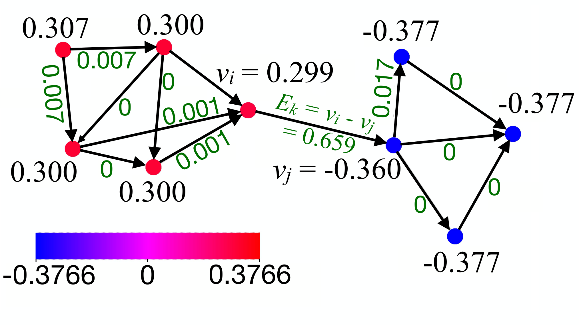
Fig. 4: Gradient example: Colors and numbers on the vertices represent the distribution corresponding to the eigenvector 𝐮1\mathbf{u}_{1} of the graph Laplacian. The direction of each edge is arbitrarily chosen. The numbers on the edges are gradients along the edges and represent elements of the vector 𝐝1=B𝖳​𝐮1\mathbf{d}_{1}=B^{\mathsf{T}}\mathbf{u}_{1}.

We denote the edge set of the graph as ℰ⁡(G)={e1,e2,⋯,em}\mathcal{E}(G)=\{e_{1},e_{2},\cdots,e_{m}\} and give every edge an arbitrary direction. For a given distribution 𝐮∈ℝn\mathbf{u}\in\mathbb{R}^{n} on the vertices, the difference of values on two vertices across an edge eke_{k} connecting vertices vi,vj∈𝒱⁡(G)v_{i},v_{j}\in{\mathcal{V}(G)} is interpreted as the “gradient” of the distribution on the graph. The gradient yields a real-valued distribution over the edge set and can thus be written as a vector 𝐝∈ℝm\mathbf{d}\in\mathbb{R}^{m} in which the kk-th element corresponds to the value on edge ek=(vi,vj)∈ℰ⁡(G)e_{k}=(v_{i},v_{j})\in\mathcal{E}(G) connecting vertices vi,vj∈𝒱⁡(G)v_{i},v_{j}\in\mathcal{V}(G) and can be expressed as dk=uj−uid_{k}=u_{j}-u_{i}. More concisely, the gradient can be written as

𝐝=B𝖳​𝐮\mathbf{d}=B^{\mathsf{T}}\mathbf{u} (5)

where 𝐮∈ℝn\mathbf{u}\in\mathbb{R}^{n} is a column vector, and B∈ℝn×mB\in\mathbb{R}^{n\times m} is the incidence matrix in which the (i,k)(i,k)-th element is defined as

Bi​k={1,if​∃ek=(vi,vj)∈ℰ⁡(G).−1,if​∃ek=(vj,vi)∈ℰ⁡(G).0,otherwise.B_{ik}=\begin{cases}1,&\text{if}~~\exists~e_{k}=(v_{i},v_{j})\in\mathcal{E}(G).\\ -1,&\text{if}~~\exists~e_{k}=(v_{j},v_{i})\in\mathcal{E}(G).\\ 0,&\text{otherwise.}\end{cases} (6)

This is illustrated in the example of Figure 4 which shows a modal distribution and the gradient values labeled on each edge. The inter-cluster edge has relatively large gradient value (0.6590.659) while the gradients over the intra-cluster edges are much smaller (order of 10−310^{-3}).

Because of the arbitrary direction assigned to edges, a gradient can be positive or negative. Thus, to identify the edges that separate the clusters, we square the individual elements of the gradient vector to obtain vector 𝐫=[d12,d22,⋯,dm2]𝖳\mathbf{r}=[d_{1}^{2},d_{2}^{2},\cdots,d_{m}^{2}]^{\mathsf{T}}, which is a positive-valued distribution over the edges. We call this the resistance vector or the resistance distribution over the edges, and it is easy to observe that it can be compactly written as

𝐫=diag​(𝐝𝐝𝖳)=diag​(B𝖳​𝐮𝐮𝖳​B)\mathbf{r}=\text{diag}(\mathbf{d}\mathbf{d}^{\mathsf{T}})=\text{diag}(B^{\mathsf{T}}\mathbf{u}\mathbf{u}^{\mathsf{T}}B) (7)

Figure 5 shows an example of the resistance vector for 𝐮1\mathbf{u}_{1}. The value of the inter-cluster edge is significantly higher and readily identified.

Refer to caption
Fig. 5: The resistance vector 𝐫1\mathbf{r}_{1} as a distribution over the edges. This resistance distribution corresponds to the gradient 𝐝1\mathbf{d}_{1} shown in Figure 4 and is computed as 𝐫1=diag​(𝐝1​𝐝1𝖳)\mathbf{r}_{1}=\text{diag}(\mathbf{d}_{1}\mathbf{d}_{1}^{\mathsf{T}}). Color on an edge indicates the resistance value on the edge.

IV-A2 Aggregated Resistance from Gradient of First qq Modes

Define the resistance vector corresponding to the ll-th mode, 𝐮l\mathbf{u}_{l}, as

𝐫l=diag​(B𝖳​𝐮l​𝐮l𝖳​B)\mathbf{r}_{l}=\text{diag}(B^{\mathsf{T}}\mathbf{u}_{l}\mathbf{u}_{l}^{\mathsf{T}}B) (8)

In order to determine all the barrier edges from the first qq modes we aggregate the resistances from the vectors 𝐫l,l=0,2,⋯,q−1\mathbf{r}_{l},l=0,2,\cdots,q-1 to define the qq-aggregated resistance as

𝐫˘\displaystyle\breve{\mathbf{r}} =\displaystyle= ∑l=0q−1𝐫l\displaystyle\sum_{l=0}^{q-1}\mathbf{r}_{l} (9)
=\displaystyle= ∑l=0q−1diag​(B𝖳​𝐮l​𝐮l𝖳​B)\displaystyle\sum_{l=0}^{q-1}\text{diag}(B^{\mathsf{T}}\mathbf{u}_{l}\mathbf{u}_{l}^{\mathsf{T}}B)
=\displaystyle= diag​(B𝖳​(∑l=0q−1𝐮l​𝐮l𝖳)​B)\displaystyle\text{diag}\left(B^{\mathsf{T}}\left(\sum_{l=0}^{q-1}\mathbf{u}_{l}\mathbf{u}_{l}^{\mathsf{T}}\right)B\right)
=\displaystyle= diag​(B𝖳​(U˘​U˘𝖳)​B)\displaystyle\text{diag}\left(B^{\mathsf{T}}\left(\breve{U}\breve{U}^{\mathsf{T}}\right)B\right)

where

U˘=[𝐮0𝐮1⋯𝐮q−1]\breve{U}=[\mathbf{u}_{0}~\mathbf{u}_{1}~\cdots~\mathbf{u}_{q-1}] (10)

is the n×qn\times q matrix with the columns corresponding to the first qq eigenvectors of LL.

Refer to caption
Fig. 6: An example of a graph, GG, with 55 well-defined clusters: All the edges of GG have the same weight of 11. With the 55-partitioned graph, 𝒢~\widetilde{\mathcal{G}}, being one with the five well-defined clusters in this graph disconnected, for this example, modaldistG​(𝒢~)=0.0035\mathrm{modaldist}_{G}(\widetilde{\mathcal{G}})=0.0035 and avgreloutG​(𝒢~)=0.6689\mathrm{avgrelout}_{G}(\widetilde{\mathcal{G}})=0.6689. For this graph n=94n=94 and λ5=4.0456\lambda_{5}=4.0456, thus satisfying the inequality of Proposition 1. From Definition 4, it is easy to check that this 𝒢~\widetilde{\mathcal{G}} is an α\alpha-realizable 55-partition for any α≥0.523\alpha\geq 0.523. The 55-aggregated resistance vector, 𝐫˘\breve{\mathbf{r}}, is also visualized in this figure as a distribution over edges – darker shade of red indicates a higher value.

Figure 6 shows an example of 𝐫˘\breve{\mathbf{r}}. The inter-cluster edges have noticeably higher values than intra-cluster edges. Once these values are computed, we can apply a threshold to values of the vector 𝐫˘\breve{\mathbf{r}} to identify the inter-cluster/bottleneck edges.

Due to Definition 1 and Proposition 1, if a graph admits a qq-partition with low avgrelout\mathrm{avgrelout}, the columns of U˘\breve{U} are close to a linear combination of the columns of U¯˘=[𝐮¯0𝐮¯1⋯𝐮¯q−1]\breve{\overline{U}}=[\overline{\mathbf{u}}_{0}~\overline{\mathbf{u}}_{1}~\cdots~\overline{\mathbf{u}}_{q-1}]. Since the columns are all orthonormal, this implies U˘≃U¯˘​R\breve{U}\simeq\breve{\overline{U}}R for some q×qq\times q orthogonal matrix RR. Thus we observe that U˘​U˘𝖳≃U¯˘​R​R𝖳​U¯˘𝖳=U¯˘​U¯˘𝖳\breve{U}\breve{U}^{\mathsf{T}}\simeq\breve{\overline{U}}RR^{\mathsf{T}}\breve{\overline{U}}^{\mathsf{T}}=\breve{\overline{U}}\breve{\overline{U}}^{\mathsf{T}} is independent of the exact nature of the linear combination. This shows that the resistance vector, 𝐫˘\breve{\mathbf{r}}, is independent of the exact nature of the linear combination of the distributions that are uniform over the subgraphs {Gj}j=0,1,⋯,q−1\{G_{j}\}_{j=0,1,\cdots,q-1} that constitute the low-eigenvalue modes (see Section III-B3). This general observation is formalized in the following proposition.

Proposition 3.

[Robustness of Resistance Vector] Consider graphs GG and G′G^{\prime} with the same topology (i.e., same vertex and edge sets, but possibly different edge weights) such that both permit the same qq-partition, 𝒢~\widetilde{\mathcal{G}}, that is α\alpha-realizable in both the graphs for some α∈[0,1)\alpha\in[0,1). Let the resistance vectors for the two graphs be 𝐫˘\breve{\mathbf{r}} and 𝐫˘′\breve{\mathbf{r}}^{\prime} respectively. Then

‖𝐫˘−𝐫˘′‖2≤2​α​2​dmax\|\breve{\mathbf{r}}-\breve{\mathbf{r}}^{\prime}\|_{2}~~\leq~~2\alpha\sqrt{2d_{\text{max}}} (11)

where dmaxd_{\text{max}} is the maximum degree over the vertices of either of the graphs.

Proof.

See Appendix -C. ∎

IV-B Approximations for Distributed Computation Without Explicit Eigendecomposition

The computation of 𝐫˘\breve{\mathbf{r}} in Equation (9) requires the computation of eigenvectors and eigenvalues, and determining how many eigenvectors (qq) to be used in computing U˘\breve{U}. In this section we propose an approximation that does not require explicit eigendecomposition of LL and is amenable to distributed computation. Furthermore, the choice of qq is replaced by the choice of a parameter, ϵ\epsilon, that is directly related to the desired value of avgreloutG​(𝒢~)\textrm{avgrelout}_{G}(\widetilde{\mathcal{G}}).

IV-B1 Approximation for Mode-independent Computation

The following proposition establishes that for a low value of qq (compared to nn) and an appropriately chosen value of ϵ\epsilon, if there exists a well-defined qq-partition of the graph, then U˘​U˘𝖳\breve{U}\breve{U}^{\mathsf{T}} can be reasonably approximated by ϵ​(ϵ​I+L)−1\epsilon(\epsilon I+L)^{-1}. We call this the approximation for mode-independent computation.

Proposition 4.

Given a desired value for an average relative outgoing weight, a^\widehat{a}, suppose there exists a qq-partition, 𝒢~\widetilde{\mathcal{G}}, such that

  • i.

    𝒢~\widetilde{\mathcal{G}} is α\alpha-realizable with some α∈[0,α^]\alpha\in[0,{\widehat{\alpha}}], and,

  • ii.

    avgreloutG​(𝒢~)∈[β​a^,a^/β]\textrm{avgrelout}_{G}(\widetilde{\mathcal{G}})\in[\beta\widehat{a},\,\widehat{a}/\beta] for some β≤1\beta\leq 1 (i.e., the actual average relative outgoing weight of the partition is within a β\beta proportion of the desired value of a^\widehat{a} in either direction).

If ϵ=2​q​a^(α^​1−α^2)1/2\epsilon={\displaystyle\frac{\sqrt{2q}~\widehat{a}}{(\widehat{\alpha}\sqrt{1-\widehat{\alpha}^{2}})^{1/2}}} , then

‖U˘​U˘𝖳−ϵ​(ϵ​I+L)−1‖2‖U˘​U˘𝖳‖2<1β​α^1−α^2\frac{\|\breve{U}\breve{U}^{\mathsf{T}}-\epsilon(\epsilon I+L)^{-1}\|_{2}}{\|\breve{U}\breve{U}^{\mathsf{T}}\|_{2}}~<~\frac{1}{\beta}{\sqrt{\frac{\widehat{\alpha}}{\sqrt{1-\widehat{\alpha}^{2}}}}}

where ∥⋅∥2\|\cdot\|_{2} is the matrix operator 22-norm.

Proof.

See Appendix G-D. ∎

As a consequence, if the graph admits a good qq-partition for a desired value of avgrelout\mathrm{avgrelout}, and if the value of ϵ\epsilon is chosen appropriately, the qq-aggregated resistance vector in (9) can be approximated as

𝐫˘≃𝐫˘aprox-I:=ϵ​diag​(B𝖳​(ϵ​I+L)−1​B)\breve{\mathbf{r}}~\simeq~\breve{\mathbf{r}}^{\text{aprox-I}}~:=~\epsilon~\text{diag}\left(B^{\mathsf{T}}(\epsilon I+L)^{-1}B\right)

This approximation automatically factors out the influence from eigenvectors corresponding to larger eigenvalues and only relies on the contribution for the first qq eigenvectors. Figure 12(b) illustrates an example in computation of the resistance vector using this approximation.

IV-B2 Approximation for Distributed Computation

The computation of the inverse of the matrix (ϵ​I+L)(\epsilon I+L), and hence the approximated resistance vector, 𝐫˘\breve{\mathbf{r}}, as described above is not immediately distributable. For distributed computation, we note that ϵ​I+L=(ϵ​I+D)−A\epsilon I+L=(\epsilon I+D)-A, where ϵ​I+D\epsilon I+D is a diagonal matrix and AA is the weighted adjacency matrix. We define the left-normalized adjacency matrix as A^ϵ=(ϵ​I+D)−1​A\widehat{A}_{\epsilon}=(\epsilon I+D)^{-1}A. (ϵ​I+L)−1(\epsilon I+L)^{-1} can then be further approximated as

(ϵ​I+L)−1=((ϵ​I+D)−A)−1=((ϵ​I+D)​(I−A^ϵ))−1=(I−A^ϵ)−1​(ϵ​I+D)−1=(∑t=0∞A^ϵt)​(ϵ​I+D)−1​(using Neumann series [16])≃(∑t=0pA^ϵt)​(ϵ​I+D)−1​(partial sum)\displaystyle\begin{array}[]{rl}&(\epsilon I+L)^{-1}\\ =&\left((\epsilon I+D)-A\right)^{-1}\\ =&\left((\epsilon I+D)(I-\widehat{A}_{\epsilon})\right)^{-1}\\ =&(I-\widehat{A}_{\epsilon})^{-1}(\epsilon I+D)^{-1}\\ =&\left(\sum_{t=0}^{\infty}\widehat{A}_{\epsilon}^{t}\right)(\epsilon I+D)^{-1}~~\text{\small{(using {Neumann series}~\cite[cite]{[\@@bibref{}{yosida2013functional}{}{}]})}}\\ \simeq&\left(\sum_{t=0}^{p}\widehat{A}_{\epsilon}^{t}\right)(\epsilon I+D)^{-1}~~\text{\small(partial sum)}\end{array}

The convergence of the infinite sum in the Neumann series above, and hence the approximation using the partial sum in the last step, is formalized in the following proposition:

Proposition 5.
  1. 1.

    ρ:=‖A^ϵ‖∞≤11+ϵ/dmax<1\rho:=\|\widehat{A}_{\epsilon}\|_{\infty}\leq\frac{1}{1+\epsilon/d_{\text{max}}}<1, where dmaxd_{\text{max}} is the maximum degree over the vertices of the graph.

  2. 2.

    Define the partial sum SN=∑t=0NA^ϵtS_{N}=\sum_{t=0}^{N}\widehat{A}_{\epsilon}^{t}. Then ‖SN‖∞<1−ρN+11−ρ\|S_{N}\|_{\infty}<\frac{1-\rho^{N+1}}{1-\rho}, ‖S∞‖∞\|S_{\infty}\|_{\infty} is bounded above by 11−ρ\frac{1}{1-\rho}, and ‖S∞−SN‖∞<ρN+11−ρ\|S_{\infty}-S_{N}\|_{\infty}<\frac{\rho^{N+1}}{1-\rho}.

Proof.

Part 1: Since the elements of A^ϵ\widehat{A}_{\epsilon} are all positive,

‖A^ϵ‖∞\displaystyle\|\widehat{A}_{\epsilon}\|_{\infty} =\displaystyle= maxi⁡(∑j[A^ϵ]i​j)\displaystyle\max_{i}\left(\sum_{j}[\widehat{A}_{\epsilon}]_{ij}\right) (19)
   (where [A^ϵ]i​j[\widehat{A}_{\epsilon}]_{ij} is the (i,j)(i,j)-th element of A^ϵ\widehat{A}_{\epsilon})
=\displaystyle= maxi⁡(∑j[(ϵ​I+D)−1​A]i​j)\displaystyle\max_{i}\left(\sum_{j}[(\epsilon I+D)^{-1}A]_{ij}\right)
=\displaystyle= maxi⁡(∑j1ϵ+deg​(vi)​Ai​j)\displaystyle\max_{i}\left(\sum_{j}\frac{1}{\epsilon+\text{deg}(v_{i})}A_{ij}\right)
=\displaystyle= maxi⁡(1ϵ+deg​(vi)​∑jAi​j)\displaystyle\max_{i}\left(\frac{1}{\epsilon+\text{deg}(v_{i})}\sum_{j}A_{ij}\right)
=\displaystyle= maxi⁡(deg​(vi)ϵ+deg​(vi))\displaystyle\max_{i}\left(\frac{\text{deg}(v_{i})}{\epsilon+\text{deg}(v_{i})}\right)
=\displaystyle= maxi⁡(11+ϵ/deg​(vi))\displaystyle\max_{i}\left(\frac{1}{1+\epsilon/\text{deg}(v_{i})}\right)
=\displaystyle= 11+ϵ/dmax\displaystyle\frac{1}{1+\epsilon/d_{\text{max}}}
<\displaystyle< 1\displaystyle 1

Part 2:

‖SN‖∞=‖∑t=0NA^ϵt‖∞\displaystyle\|S_{N}\|_{\infty}~=~\left\|\sum_{t=0}^{N}\widehat{A}_{\epsilon}^{t}\right\|_{\infty} ≤\displaystyle\leq ∑t=0N‖A^ϵ‖∞t\displaystyle\sum_{t=0}^{N}\|\widehat{A}_{\epsilon}\|_{\infty}^{t} (20)
=\displaystyle= ∑t=0Nρt=1−ρN+11−ρ\displaystyle\sum_{t=0}^{N}\rho^{t}~=~\frac{1-\rho^{N+1}}{1-\rho}

Thus, limN→∞‖SN‖∞≤11−ρ\lim_{N\rightarrow\infty}\|S_{N}\|_{\infty}\leq\frac{1}{1-\rho}.

Furthermore,

‖S∞−SN‖∞\displaystyle\|S_{\infty}-S_{N}\|_{\infty} =\displaystyle= ‖∑t=N+1∞A^ϵt‖∞=‖A^ϵN+1​∑t=0∞A^ϵt‖∞\displaystyle\left\|\sum_{t=N+1}^{\infty}\widehat{A}_{\epsilon}^{t}\right\|_{\infty}~=~\left\|\widehat{A}_{\epsilon}^{N+1}\sum_{t=0}^{\infty}\widehat{A}_{\epsilon}^{t}\right\|_{\infty} (21)
≤\displaystyle\leq ρN+1​∑t=0∞ρt=ρN+11−ρ\displaystyle\rho^{N+1}\sum_{t=0}^{\infty}\rho^{t}~=~\frac{\rho^{N+1}}{1-\rho}

Thus the partial sums, SNS_{N}, get closer to S∞S_{\infty} exponentially fast as the value of NN increases. ∎

The consequence of the above proposition is that the qq-aggregated resistance vector can be further approximated as

𝐫˘aprox-II:=ϵ​diag​(B𝖳​(∑t=0pA^ϵt)​(ϵ​I+D)−1​B)\breve{\mathbf{r}}^{\text{aprox-II}}~:=~\epsilon~\text{diag}\left(B^{\mathsf{T}}\left(\sum_{t=0}^{p}\widehat{A}_{\epsilon}^{t}\right)(\epsilon I+D)^{-1}B\right)

where A^ϵ=(ϵ​I+D)−1​A\widehat{A}_{\epsilon}=(\epsilon I+D)^{-1}A. We next discuss how the computation of 𝐫˘aprox-II\breve{\mathbf{r}}^{\text{aprox-II}} can be distributed over the graph.

Since (ϵ​I+D)(\epsilon I+D) is a diagonal matrix and AA is the adjacency matrix, the computation of the tt-th power of A^ϵ=(ϵ​I+D)−1​A\widehat{A}_{\epsilon}=(\epsilon I+D)^{-1}A is amenable to distributed computation. In order to describe the distributed computation algorithm we observe that the (i,j)(i,j)-th element of A^ϵt+1\widehat{A}_{\epsilon}^{t+1} can be written as

[A^ϵt+1]i​j\displaystyle[\widehat{A}_{\epsilon}^{t+1}]_{ij} =\displaystyle= ∑l[A^ϵ]i​l​[A^ϵt]l​j\displaystyle\sum_{l}[\widehat{A}_{\epsilon}]_{il}~[\widehat{A}_{\epsilon}^{t}]_{lj} (22)
=\displaystyle= ∑{l|vl∈𝒩G​(vi)}[A^ϵ]i​l​[A^ϵt]l​j\displaystyle{\sum_{{\{l|v_{l}\in\mathscr{N}_{G}(v_{i})\}}}[\widehat{A}_{\epsilon}]_{il}~[\widehat{A}_{\epsilon}^{t}]_{lj}}
=\displaystyle= ∑{l|vl∈𝒩G​(vi)}Ai​lϵ+Di​i​[A^ϵt]l​j\displaystyle{\sum_{{\{l|v_{l}\in\mathscr{N}_{G}(v_{i})\}}}\frac{A_{il}}{\epsilon+D_{ii}}~[\widehat{A}_{\epsilon}^{t}]_{lj}}

where 𝒩G​(vi)={vj|(vi,vj)∈ℰ⁡(G)}\mathscr{N}_{G}{(v_{i})=\{v_{j}\,|\,(v_{i},v_{j})\in\mathcal{E}(G)\}} indicates the set of vertices that are neighbors of the ii-th vertex. The second equality in (22) holds because [A^ϵ]i​l[\widehat{A}_{\epsilon}]_{il} is non-zero only if (vi,vl)∈ℰ⁡(G)(v_{i},v_{l})\in\mathcal{E}(G).

In a distributed computation, the vertex ii will store only the elements of the ii-th row of A^ϵt\widehat{A}_{\epsilon}^{t} and the computation of the ii-th row of the partial sum matrix, S​p:=∑t=0pA^ϵtS\!p:=\sum_{t=0}^{p}\widehat{A}_{\epsilon}^{t}. In practice each vertex can maintain associative arrays for the rows, which are populated as new non-zero entries are computed. This is illustrated in Algorithm 1.

Algorithm 1 Distributed computation of ii-th row of the partial sum S​pS\!p, and the resistance values on the edges emanating from viv_{i}.

Inputs: i. (i,l)(i,l)-th element of Adjacency Matrix, 𝖠i​l​∀{l|vl∈𝒩G​(vi)}\mathsf{A}_{il}~\forall~{\{l\,|\,v_{l}\in\mathscr{N}_{G}(v_{i})\}};  ii. Degree of the vertex, 𝖣i\mathsf{D}_{i};  iii. ϵ\epsilon.

Outputs: i. Associative array 𝖲𝗉i\mathsf{Sp}_{i} representing ii-th row of S​pS\!p; ii. For every {l|vl∈𝒩G​(vi)}{\{l\,|\,v_{l}\in\mathscr{N}_{G}(v_{i})\}}, the value of the resistance 𝗋˘aprox-II​[i,l]\breve{\mathsf{r}}^{\text{aprox-II}}[i,l] on the edge (vi,vl)(v_{i},v_{l}).

1: Associative array 𝖠^​𝖯𝗈𝗐i←{(i:1)}\mathsf{\widehat{A}Pow}_{i}\leftarrow\{(i\!:1)\}   // identity matrix
2: 𝗍i←0\mathsf{t}_{i}\leftarrow 0   // iteration number for data in 𝖠^​𝖯𝗈𝗐i\mathsf{\widehat{A}Pow}_{i}
3: Associative array 𝖠^​𝖯𝗈𝗐𝖳𝗆𝗉i←{}\mathsf{\widehat{A}PowTmp}_{i}\leftarrow\{\}
4: 𝖽𝗈𝗇𝖾i←0\mathsf{done}_{i}\leftarrow 0   // iteration number for data in 𝖠^​𝖯𝗈𝗐𝖳𝗆𝗉i\mathsf{\widehat{A}PowTmp}_{i}
5: Associative array 𝖲𝗉i←{}\mathsf{Sp}_{i}\leftarrow\{\}
6: Associative array 𝗋˘aprox-II←{}\breve{\mathsf{r}}^{\text{aprox-II}}\leftarrow\{\}
7: while 𝗍i<p\mathsf{t}_{i}<p do
8:   for {l|vl∈𝒩G​(vi)}{\{l\,|\,v_{l}\!\in\!\mathscr{N}_{G}(v_{i})\}} do   // communicate w/neighbors
9:    while 𝗍l<𝗍i\mathsf{t}_{l}<\mathsf{t}_{i} do wait   // wait for latest data    
10:    for (j:𝗌j)∈𝖠^​𝖯𝗈𝗐l(j\!:{\mathsf{s}_{j}})\in\mathsf{\widehat{A}Pow}_{l} do
11:      𝖠^​𝖯𝗈𝗐𝖳𝗆𝗉i​[j]←𝖠i​lϵ+𝖣i∗𝗌j\mathsf{\widehat{A}PowTmp}_{i}[j]\leftarrow\frac{\mathsf{A}_{il}}{\epsilon+\mathsf{D}_{i}}*{\mathsf{s}_{j}}      
12:   𝖽𝗈𝗇𝖾i←𝗍i+1\mathsf{done}_{i}\leftarrow\mathsf{t}_{i}+1
13:   for {l|vl∈𝒩G​(vi)}{\{l\,|\,v_{l}\!\in\!\mathscr{N}_{G}(v_{i})\}} do   // wait for neighbors
14:    while 𝖽𝗈𝗇𝖾l<𝗍i+1\mathsf{done}_{l}<\mathsf{t}_{i}+1 do wait      𝖠^​𝖯𝗈𝗐i←𝖠^​𝖯𝗈𝗐𝖳𝗆𝗉i\mathsf{\widehat{A}Pow}_{i}\leftarrow\mathsf{\widehat{A}PowTmp}_{i}
15:   𝗍i←𝗍i+1\mathsf{t}_{i}\leftarrow\mathsf{t}_{i}+1
16:   for (j:𝗌j)∈𝖠^​𝖯𝗈𝗐i(j\!:\mathsf{s}_{j})\in\mathsf{\widehat{A}Pow}_{i} do   // update partial sum
17:    if 𝖲𝗉i​[j]\mathsf{Sp}_{i}[j] does not exist then
18:      𝖲𝗉i​[j]←𝗌j\mathsf{Sp}_{i}[j]\leftarrow\mathsf{s}_{j}
19:    else
20:      𝖲𝗉i​[j]←𝖲𝗉i​[j]+𝗌j\mathsf{Sp}_{i}[j]\leftarrow\mathsf{Sp}_{i}[j]+\mathsf{s}_{j}      
21: for {l|vl∈𝒩G​(vi)}{\{l\,|\,v_{l}\!\in\!\mathscr{N}_{G}(v_{i})\}} do   // wait for neighbors
22:   while 𝗍l<p\mathsf{t}_{l}<p do wait   
23: for {l|vl∈𝒩G​(vi)}{\{l\,|\,v_{l}\!\in\!\mathscr{N}_{G}(v_{i})\}} do   // communicate w/neighbors
24:   𝗋˘aprox-II​[i,l]←ϵ⁡(𝖲𝗉i​[i]−𝖲𝗉l​[i]ϵ+𝖣i+ϵ​𝖲𝗉l​[l]−𝖲𝗉i​[l]ϵ+𝖣l)\breve{\mathsf{r}}^{\text{aprox-II}}[i,l]\leftarrow\epsilon\left(\frac{\mathsf{Sp}_{i}[i]-\mathsf{Sp}_{l}[i]}{\epsilon+\mathsf{D}_{i}}+\frac{\epsilon\mathsf{Sp}_{l}[l]-\mathsf{Sp}_{i}[l]}{\epsilon+\mathsf{D}_{l}}\right)

Suppose the kk-th edge connects the ii-th to the ll-th vertex (i.e., vl∈𝒩G​(vi)v_{l}\in\mathscr{N}_{G}(v_{i}) and ek=(vi,vl)∈ℰ⁡(G)e_{k}=(v_{i},v_{l})\in\mathcal{E}(G)). Using the ii- and ll-th rows of the partial sum matrix, S​pS\!p, stored on vertices ii and ll respectively, and using their respective degrees, the resistance on the edge (the kk-th component of the resistance vector) can be computed in a distributed manner as follows:

r˘k\displaystyle\breve{r}_{k} ≃\displaystyle\simeq r˘kaprox-II\displaystyle\breve{r}_{k}^{\text{aprox-II}} (23)
:⁣=\displaystyle:= ϵ​[B𝖳​(∑t=0pA^ϵt)​(ϵ+D)−1​B]k​k\displaystyle\epsilon\left[B^{\mathsf{T}}\left(\sum_{t=0}^{p}\widehat{A}_{\epsilon}^{t}\right)(\epsilon+D)^{-1}B\right]_{kk}
=\displaystyle= ϵ​∑a,bBa​k​S​pa​b​1ϵ+Db​b​Bb​k\displaystyle\epsilon\sum_{{a,b}}B_{ak}~{S\!p}_{ab}~\frac{1}{\epsilon+D_{bb}}~B_{bk}
=\displaystyle= ϵ​∑a,b∈{i,l}Ba​k​S​pa​b​1ϵ+Db​b​Bb​k\displaystyle\epsilon\sum_{a,b\in\{i,l\}}B_{ak}~{S\!p}_{ab}~\frac{1}{\epsilon+D_{bb}}~B_{bk}
=\displaystyle= ϵ​S​pi​iϵ+Di​i−ϵ​S​pl​iϵ+Di​i+ϵ​S​pl​lϵ+Dl​l−ϵ​S​pi​lϵ+Dl​l\displaystyle\frac{\epsilon{S\!p}_{ii}}{\epsilon+D_{ii}}-\frac{\epsilon{S\!p}_{li}}{\epsilon+D_{ii}}+\frac{\epsilon{S\!p}_{ll}}{\epsilon+D_{ll}}-\frac{\epsilon{S\!p}_{il}}{\epsilon+D_{ll}}\quad

where the first approximation follows from Equation (9), Proposition 4 and Equation (IV-B2), and the simplification of the summation domain from every pair of vertex indices to {i,l}\{i,l\} is due to the fact that Bc​kB_{ck} is zero for any c∉{i,l}c\notin\{i,l\}. The important thing to note here is that this approximate computation of the resistance on the kk-th edge requires only values stored on its bounding vertices, thus making this computation distributable as well. The complete algorithm for the distributed computation of the resistances is described in Algorithm 1.

Figure 12(c) illustrates a result in computation of the resistance vector using this distributed implementation.

V Inter-cluster Transmission Rate Control Using Modal Barriers

V-A Transmission Model

Refer to caption
Fig. 7: Example of start and target vertices for transmission. This figure shows the setup for the simulation result in Figure 9.

For a given graph and weighted Laplacian matrix, L′=D′−A′L^{\prime}=D^{\prime}-A^{\prime} (where A′A^{\prime} is the weighted adjacency matrix, and D′D^{\prime} the corresponding diagonal degree matrix), consider the following dynamics on the graph

𝐱˙=−L′​𝐱\dot{\mathbf{x}}=-L^{\prime}\mathbf{x} (24)

where 𝐱∈ℝn\mathbf{x}\in\mathbb{R}^{n} corresponds to a distribution over the vertices of the graph.

A first-order discrete time form of equation (24) can be written as

𝐱⁡(τ+Δ​τ)\displaystyle\mathbf{x}(\tau+\Delta\tau) =\displaystyle= (I−Δ​τ​L)​𝐱​(τ)\displaystyle(I-\Delta\tau~L)\mathbf{x}(\tau)
or more simply,𝐱(t+1)\displaystyle\text{or more simply,}\quad\mathbf{x}^{(t+1)} =\displaystyle= (I−κ​L)​𝐱(t)\displaystyle(I-\kappa L)\mathbf{x}^{(t)} (25)

where τ∈ℝ\tau\in\mathbb{R} is the continuous time, while t∈ℤt\in\mathbb{Z} is the (re-scaled) discrete time. κ≪2λn\kappa\ll\frac{2}{\lambda_{n}} is a small number chosen to ensure that (I−κ​L)(I-\kappa L) has the same eigenspace as LL, but its highest eigenvalue is 11 corresponding to the eigenvector 𝐮0\mathbf{u}_{0}, while all other eigenvalues are in (−1,1)(-1,1).

As t→+∞t\rightarrow+\infty, 𝐱(+∞)\mathbf{x}^{(+\infty)} thus converges to the first eigenvector, 𝐮0\mathbf{u}_{0}, of LL, which corresponds to a uniform distribution over the vertices. The effect of the dynamics is diffusion – starting with any non-zero distribution 𝐱(0)\mathbf{x}^{(0)}, the dynamics of (24) or (V-A) ends up re-distributing the values on the vertices to their neighbors until an equilibrium (uniform distribution) is attained. In fact the dynamics in (24) can be written as

x˙i=−(Di′​xi−∑{j|(vi,vj)∈ℰ(G)}Ai​j′​xj)=∑{j|vj∈𝒩G(vi)}Ai​j′​xj−(∑{j|vj∈𝒩G(vi)}Ai​j′)​xi\begin{array}[]{rcl}\dot{x}_{i}&=&\displaystyle-(D^{\prime}_{i}x_{i}~-\!\!\!\!\sum_{\{j|\atop(v_{i},v_{j})\in\mathcal{E}(G)\}}\!\!\!\!A^{\prime}_{ij}x_{j})\\ &=&\displaystyle\!\!\!\!\sum_{\{j|\atop v_{j}\in\mathscr{N}_{G}(v_{i})\}}\!\!\!\!A^{\prime}_{ij}x_{j}~-~\left(\sum_{\{j|\atop v_{j}\in\mathscr{N}_{G}(v_{i})\}}\!\!\!\!A^{\prime}_{ij}\right)x_{i}\end{array} (26)

In this form it’s easy to see that the diffusion rate from vjv_{j} to viv_{i} (i.e., across the edge (vi,vj)(v_{i},v_{j})) is determined by the weight on the edge, Ai​j′A^{\prime}_{ij} (the (i,j)(i,j)-th element of the weighted adjacency matrix). The lower the rate, the slower the diffusion across the edge. Furthermore, it is clear that the dynamics required only neighborhood communication/transmission, since updating xix_{i} requires the values of xjx_{j} for only the neighbor indices in {j|vj∈𝒩G​(vi)}\{j\,|\,v_{j}\in\mathscr{N}_{G}(v_{i})\}.

We thus use this as a model for network transmission (such as information in a communication network context, or infection in context of disease spread) in the network. The entity being transmitted is represented by the values of the elements of 𝐱\mathbf{x}, with XkX_{k} denoting the value on vertex vkv_{k}.

In particular we consider the situation where the entity being transmitted originates from one particular start vertex, v𝗌𝗍𝖺𝗋𝗍v_{\mathsf{start}} (i.e., the kk-th element of 𝐱(0)\mathbf{x}^{(0)} is xk(0)=1,when​k=s,or​xk(0)=0​otherwise.x_{k}^{(0)}=1,\text{when}~k=s,~\text{or}~x_{k}^{(0)}=0~\text{otherwise}.). We are interested in studying (and reducing) the time taken by the dynamics to make the value on a target vertex, v𝗍𝖺𝗋𝗀𝖾𝗍v_{\mathsf{target}} (belonging to a different cluster than v𝗌𝗍𝖺𝗋𝗍v_{\mathsf{start}}), go above a threshold value of γ\gamma, And we refer to the value of the target vertex v𝗍𝖺𝗋𝗀𝖾𝗍v_{\mathsf{target}} as x𝗍𝖺𝗋𝗀𝖾𝗍x_{\mathsf{target}}. Figure 7 shows an example of start and target vertices for transmission on a simple graph.

V-B Edge Weight Computation

For the edge weights modeling the dynamics (elements of the weighted adjacency matrix that govern the dynamics (26)) we consider three different cases:

  • i.

    Unrestricted Transmission: In this case we set a uniform unit weight for every edge in the graph. The corresponding adjacency matrix, degree matrix and the Laplacian matrix are denoted by AU,DUA^{U},D^{U} and LUL^{U}. The (continuous-time) dynamics of unrestricted transmission is thus 𝐱˙=−LU​𝐱\dot{\mathbf{x}}=-L^{U}\mathbf{x}.

  • ii.

    Inter-cluster Barriered Transmission: In order to reduce transmission across the network we propose to decrease weights on selected edges (reducing the rate of transmission across those edges). For this approach, we use the resistance vector computed using the Laplacian for unrestricted transmission, LUL^{U}, to compute new weights. In particular, if r˘k\breve{r}_{k} is the resistance computed for the kk-th edge, we define the new barrier weights as

    wkB=ϵBϵB+r˘kw^{B}_{k}=\frac{\epsilon_{B}}{\epsilon_{B}+\breve{r}_{k}} (27)

    where 0<ϵB≪10<\epsilon_{B}\ll 1 is a small positive constant. These barrier weights thus take values in (0,1](0,1] and edges with computed resistance close to 00 (such as the intra-cluster edges) have barrier weights close to 11, while the barrier weights are lower for edges on which the computed resistance is high (for example the inter-cluster edges) 33 3 Note that a lower weight implies lower transmission rate across an edge, and hence constitutes a barrier, while weights closer to 11 correspond to less restricted transmission.. The corresponding adjacency matrix, degree matrix and Laplacian are thus

    Ai​jB\displaystyle A^{B}_{ij} =\displaystyle= {wkB,if ​∃ek=(vi,vj)∈ℰ⁡(G)​ or ∃ek=(vj,vi)∈ℰ⁡(G)0,otherwise.\displaystyle\left\{\begin{array}[]{l}w^{B}_{k},~~\text{if }\exists~e_{k}=(v_{i},v_{j})\in\mathcal{E}(G)\text{ or }\\ \qquad\qquad\exists~e_{k}=(v_{j},v_{i})\in\mathcal{E}(G)\\ 0,~~\text{otherwise.}\end{array}\right.
    DB\displaystyle D^{B} =\displaystyle= diagj​(∑i=1nAi​jB)\displaystyle\mathrm{diag}_{j}\left(\sum_{i=1}^{n}A^{B}_{ij}\right)
    LB\displaystyle L^{B} =\displaystyle= DB−AB\displaystyle D^{B}-A^{B} (32)

    The (continuous-time) dynamics of transmission with inter-cluster barrier is then defined as 𝐱˙=−LB​𝐱\dot{\mathbf{x}}=-L^{B}\mathbf{x}.

  • iii.

    Shuffled Weight Transmission: In order to be able to compare/benchmark the performance of the barriered transmission described above, we randomly shuffle the barrier weights as computed in (27) across the different edges of the graph. We define shuffled weight on the kk-th edge as wkS=wσ⁡(k)Bw^{S}_{k}=w^{B}_{\sigma(k)}, for some permutation, σ\sigma, of (1,2,⋯,m)(1,2,\cdots,m). The corresponding adjacency matrix, degree matrix and Laplacian matrix are denoted by AS,DSA^{S},D^{S} and LSL^{S}, and the (continuous-time) dynamics of transmission with shuffled weights is defined as 𝐱˙=−LS​𝐱\dot{\mathbf{x}}=-L^{S}\mathbf{x}.

    If we regard decreasing the weight on an edge below 1 as consuming a certain amount of available resource, the simple shuffling of the weights ensure that the same amount of resource is being used in lowering the weights (i.e., the same number of edges with the same weights as in the barrierred transmission case), but the edges are chosen randomly without using our method for mode-based barrier construction. This gives a baseline method to compare against.

VI Results

VI-A Inter-cluster Edge Detection Comparison

We compare the performance of our method in detecting inter-cluster edges with a recent algorithm [2] based on multiway Cheeger partitioning that uses an integer linear programming formulation to find partitions. For this algorithm, the number of clusters is required as input and, for a total of qq clusters and nn vertices, the first q−1q-1 clusters are required to contain less than an average of n/qn/q vertices. This requirement affects the accuracy of the bottleneck detection as shown in the example of Figure 8. In this case, some vertices are forced to be separated from their well-aggregated cluster due to the vertex count limit per cluster, resulting in sub-optimal inter-cluster edge detection. Furthermore, because of the integer linear programming implementation, the multiway Cheeger partition algorithm took 54,304.654,304.6 seconds to compute the partitions in this particular example on an intel cpu. In comparison, our method took less than one second to compute the resistance, 𝐫˘\breve{\mathbf{r}}, on the edges using (9), and the result is shown in Figure 6.

Refer to caption
Fig. 8: Detected bottleneck edges using the multiway Cheeger partition algorithm [2]. The method is less accurate in clustering and significantly more computationally complex than our proposed resistance computation, illustrated in Figure  6 (see text Section VI-A).

VI-B Transmission Rate

Fig. 9: Discrete time simulations of information transmission using the setup of Figure 7. The barriered transmission slows the information conveyed across the network from start to target (see the example description, Section VI-B ).

A comparison of transmission rates using the different weight assignment methods described in Section V-B is shown in Figure 9. As can be seen from the plot, the value of x𝗍𝖺𝗋𝗀𝖾𝗍{x_{\mathsf{target}}} grows significantly slower when using the Barriered transmission weights than using the Unrestricted transmission weights or the Shuffled weights. While eventually any non-zero weights will result in convergence to a uniform distribution (corresponding to the null-space vector of either of LUL^{U}, LBL^{B} or LSL^{S}), the objective of slowing the rate of transmission using the barriered weights is clearly achieved.

Fig. 10: First (smallest) 8 eigenvalues of the graph Laplacian of ego-Facebook network
Fig. 11: Discrete time simulations of information transmission in the ego-Facebook network.

For a large scale network graph example, we use an open network dataset called ego-Facebook from the Stanford Large Network Dataset Collection [10]. This anonymized social network has 40394039 nodes and 8823488234 edges in total. As shown is Figure 10, there is a big gap between λ6\lambda_{6} and λ7\lambda_{7} for this network. We choose q=7q=7 in Equation (10) to construct our barrier weighted graph Laplacian. We also choose node #​1\#1 as the start vertex and node #​4038\#4038 as the target vertex for information transmission across the network. The simulation result in Figure 11 shows a similar trend as the result of the small scale simulation (Figure 9). The barrier edge weights are able to slow the information transmission effectively.

VI-C Comparison of Approximate Methods for Distributed Computation

We use 33 different methods for computing U˘​U˘𝖳\breve{U}\breve{U}^{\mathsf{T}} for computing the resistance vector, 𝐫˘\breve{\mathbf{r}}, in equation (9). The first is the direct eigen-decomposition of the graph Laplacian for computing U˘\breve{U}. The second is the approximate method for mode-independent computation as was described under Section IV-B1. And finally we use the approximation method for distributed computation as was described in Section IV-B2.

Refer to caption
((a)) Direct computation of 𝐫˘\breve{\mathbf{r}}.
Refer to caption
((b)) Approximation for mode-independent computation for computing 𝐫˘aprox-I\breve{\mathbf{r}}_{\text{aprox-I}}.
Refer to caption
((c)) Approximation for distributed computation for computing 𝐫˘aprox-II\breve{\mathbf{r}}_{\text{aprox-II}}.
Fig. 12: A qualitative comparison of accuracy in computing 𝐫˘\breve{\mathbf{r}}. ϵ=0.1\epsilon=0.1 is chosen in the approximation for mode-independent computation. p=N2p=\frac{N}{2} is chosen for the distributed approximation approach. The resulting L​2L2 norms:‖𝐫˘aprox-I−𝐫˘‖=0.095:\|\breve{\mathbf{r}}_{\text{aprox-I}}-\breve{\mathbf{r}}\|=0.095 and ‖𝐫˘aprox-II−𝐫˘‖=1.076\|\breve{\mathbf{r}}_{\text{aprox-II}}-\breve{\mathbf{r}}\|=1.076.

Figure 12 shows the results obtained on a simple graph using these three methods. As can be seen from the value of ‖𝐫˘aprox-I−𝐫˘‖\|\breve{\mathbf{r}}_{\text{aprox-I}}-\breve{\mathbf{r}}\|, the result using the approximation methods for mode-independent computation is very close to the direct computation. The advantage of the approximation is that it can be computed in a decentralized manner, which is especially useful when dealing with a large scale graph whose nodes have limited computational resources and communicate only with edge-connected neighbors.

VI-D Pandemic simulation

Fig. 13: Simulation results of the number of people infected using unrestricted weights, barrier weights (inter-cluster restrictions) and shuffled weights. For each day, the number of people infected is averaged over 10001000 simulations (each simulation has randomized initial patient-zero).
Refer to caption
((a)) Day 1
Refer to caption
((b)) Day 30
Refer to caption
((c)) Day 60
Refer to caption
((d)) Day 90
Refer to caption
((e)) Day 1
Refer to caption
((f)) Day 45
Refer to caption
((g)) Day 90
Refer to caption
((h)) Day 135
Fig. 14: Snapshots of the viral spread simulation. (a), (b), (c) and (d) are snapshots from the simulation without social restrictions; (e), (f), (g) and (h) are snapshots from the simulation with inter-cluster social restrictions using barrier weights.

As of writing this paper, our world is undergoing the COVID-19 pandemic. Social restriction has been shown to be a proven way of slowing the spread of the virus and providing time for treatment and eradication measures [12]. From our previous simulations, we can already see how effective the graph modal barriers are for slowing transmission across a network. We thus apply the method developed in this paper to a pandemic model that can lower the probability of virus transmission along inter-cluster connections. In this context a cluster can be a representation of a closely-knit community of individuals (e.g, with a vertex representing a household and the flow representing interaction/travel of individuals). Thus, given limited resources for imposing restrictions on travel or social interactions, identifying the most critical edges that predominate in transmitting the virus from one community to another (as is done by the proposed modal barrier method) is essential.

For the simulation, the daily contagious probability of the kk-th edge, ek=(vi,vj)e_{k}=(v_{i},v_{j}) (i.e., the probability that vjv_{j} will get infected if viv_{i} is infected), is assumed to be

Pk=wk′​PaP_{k}=w^{\prime}_{k}P_{a} (33)

where PaP_{a} is a constant which is set to be 0.030.03. The lower the weight on the kk-th edge, the lower is the probability of transmission.

Initially we start with only one infected vertex (“patient zero”). Once infected, a vertex will turn contagious in a range of 33 to 55 days, and will stay infected for a range of 1515 to 7070 days. We compare the results with uniform unrestricted weights, wkU(=1​∀k)w^{U}_{k}(=1~\forall k), barriered weights, wkBw^{B}_{k}, and shuffled weights, wkSw^{S}_{k}.

Results for the ego-Facebook network are shown in Figure 13. Figure 14 shows some snapshots on the spread of the infection across the example graph shown in Figure 6.

VII Conclusion

In this paper we used the eigenvectors of the graph Laplacian to construct modal barrier weights on the edges of a graph to lower the transmission rate on those critical edges. Our method relies on using the eigenvectors to identify clusters in the graph and hence the edges that form weak inter-cluster connections form the basis of preventing inter-cluster transmission. We provided theoretical foundations for the proposed method and developed an approximation that enabled low complexity distributed computation of the barrier weights. We demonstrated that the proposed method is more effective in slowing transmission across a network compared to a method that uses the same amount of resources in lowering the edge weights but does so in a randomized manner. We discussed the applicability of the proposed method in deciding how to impose social distancing and travel restrictions in preventing transmission of infection across communities.

-A Proof of Proposition 1

We use the same notations as in Definition 1, Definition 2 and Proposition 1.

Lemma 1.
2​reloutG​(Gj)≥‖(L−L¯)​𝐮¯j‖2\sqrt{2}~\mathrm{relout}_{G}(G_{j})~\geq~\|(L-\overline{L})\overline{\mathbf{u}}_{j}\|_{2}

Lemma 1 ​​​​​​​​​​​​

Proof.

Suppose DkD_{k} and D¯k\overline{D}_{k} are the degrees of the vertex vk∈𝒱⁡(Gj)v_{k}\in\mathcal{V}(G_{j}) in the graphs GG and G¯\overline{G} respectively. Then DkD_{k} and D¯k\overline{D}_{k} are equal iff all the neighbors of vkv_{k} are in GjG_{j}. Otherwise Dk−D¯kD_{k}-\overline{D}_{k} is the net outgoing degree of the vertex vkv_{k} from the sub-graph GjG_{j}. That is, if vk∈𝒱⁡(Gj)v_{k}\in\mathcal{V}(G_{j}),

Dk−D¯k\displaystyle D_{k}-\overline{D}_{k} =\displaystyle= ∑{l|vl∈𝒱(Gi),i≠j}Ak​l\displaystyle\sum_{\{l\,|\,v_{l}\in\mathcal{V}(G_{i}),i\neq j\}}A_{kl} (34)

Suppose AA and A¯\overline{A} are the adjacency matrices of GG and G¯\overline{G}. An edge (vk,vl)(v_{k},v_{l}) exists (and have the same weight, i.e., Ak​l=A¯k​lA_{kl}=\overline{A}_{kl}) in both GG and G¯\overline{G} iff vkv_{k} and vlv_{l} belong to the same sub-graph. Otherwise A¯k​l=0\overline{A}_{kl}=0 (the edge is non-existent in G¯\overline{G}). Thus,

Ak​l−A¯k​l={Ak​l,if vk∈𝒱⁡(Gj),vl∈𝒱⁡(Gi),i≠j0,otherwise.A_{kl}-\overline{A}_{kl}~=~\left\{\begin{array}[]{l}A_{kl},~\text{if $v_{k}\in\mathcal{V}(G_{j}),v_{l}\in\mathcal{V}(G_{i}),i\neq j$}\\ 0,~~\text{otherwise.}\end{array}\right. (35)

Next we consider the vector 𝐮¯j\overline{\mathbf{u}}_{j} (for j=0,1,⋯,q−1j=0,1,\cdots,q-1), which by definition is non-zero and uniform only on vertices in the sub-graph GjG_{j}. Let u¯l​j\overline{u}_{lj} be the ll-th element of the unit vector 𝐮¯j\overline{\mathbf{u}}_{j}. Thus,

u¯l​j={1|𝒱⁡(Gj)|,if vl∈𝒱⁡(Gj)0,otherwise\overline{u}_{lj}=\left\{\begin{array}[]{l}\frac{1}{\sqrt{|\mathcal{V}(G_{j})|}},~~\text{if $v_{l}\in\mathcal{V}(G_{j})$}\\ 0,~~\text{otherwise}\end{array}\right. (36)

Thus the kk-th element of the vector (L−L¯)​𝐮¯j(L-\overline{L})\overline{\mathbf{u}}_{j},

[(L−L¯)​𝐮¯j]k\displaystyle[(L-\overline{L})\overline{\mathbf{u}}_{j}]_{k}
=\displaystyle= ∑l(Dk​l−Ak​l−D¯k​l+A¯k​l)​u¯l​j\displaystyle\displaystyle\sum_{l}(D_{kl}-A_{kl}-\overline{D}_{kl}+\overline{A}_{kl})\overline{u}_{lj}
=\displaystyle= (Dk−D¯k)​u¯k​j−∑l(Ak​l−A¯k​l)​u¯l​j\displaystyle\displaystyle(D_{k}-\overline{D}_{k})\overline{u}_{kj}-\sum_{l}(A_{kl}-\overline{A}_{kl})\overline{u}_{lj}
            (since DD and D¯\overline{D} are diagonal marices)
=\displaystyle= (1|𝒱⁡(Gj)|​{(Dk−D¯k),if vk∈𝒱⁡(Gj)0,otherwise)\displaystyle\displaystyle\left(\frac{1}{\sqrt{|\mathcal{V}(G_{j})|}}\left\{\begin{array}[]{l}(D_{k}-\overline{D}_{k}),~\text{if $v_{k}\in\mathcal{V}(G_{j})$}\\ 0,~\text{otherwise}\end{array}\right.\right)
−(1|𝒱⁡(Gj)|​∑{l|vl∈𝒱⁡(Gj)}(Ak​l−A¯k​l))\displaystyle\displaystyle\hskip 18.49988pt\hskip 18.49988pt-\left(\frac{1}{\sqrt{|\mathcal{V}(G_{j})|}}\sum_{\{l\,|\,v_{l}\in\mathcal{V}(G_{j})\}}(A_{kl}-\overline{A}_{kl})\right)
                  (using the definition of u¯l​j\overline{u}_{lj})
=\displaystyle= 1|𝒱⁡(Gj)|({∑{l|vl∈𝒱(Gi),i≠j}Ak​l,if vk∈𝒱⁡(Gj)0,otherwise\displaystyle\displaystyle\frac{1}{\sqrt{|\mathcal{V}(G_{j})|}}\left(\left\{\begin{array}[]{l}\displaystyle\sum_{\{l\,|\,v_{l}\in\mathcal{V}(G_{i}),i\neq j\}}\!\!A_{kl},~~~\text{if $v_{k}\in\mathcal{V}(G_{j})$}\\ 0,\hskip 18.49988pt\hskip 18.49988pt\text{otherwise}\end{array}\right.\right.
−∑{l|vl∈𝒱⁡(Gj)}{Ak​l,if vk∈𝒱⁡(Gi),i≠j0,otherwise.)\displaystyle\displaystyle\hskip 18.49988pt\hskip 18.49988pt-\left.\sum_{\{l\,|\,v_{l}\in\mathcal{V}(G_{j})\}}\left\{\begin{array}[]{l}A_{kl},~~\text{if $v_{k}\in\mathcal{V}(G_{i}),i\neq j$}\\ 0,~\text{otherwise.}\end{array}\right.\right)
                     (using (34) and (35))
=\displaystyle= 1|𝒱⁡(Gj)|​{∑{l|vl∈𝒱(Gi),i≠j}Ak​l,if vk∈𝒱⁡(Gj)−∑{l|vl∈𝒱⁡(Gj)}Ak​l,if vk∈𝒱⁡(Gi),i≠j\displaystyle\displaystyle\frac{1}{\sqrt{|\mathcal{V}(G_{j})|}}\left\{\begin{array}[]{l}\displaystyle\sum_{\{l\,|\,v_{l}\in\mathcal{V}(G_{i}),i\neq j\}}\!\!\!\!A_{kl},~~~\text{if $v_{k}\in\mathcal{V}(G_{j})$}\\ \displaystyle-\sum_{\{l\,|\,v_{l}\in\mathcal{V}(G_{j})\}}A_{kl},~~~~~\text{if $v_{k}\in\mathcal{V}(G_{i}),i\neq j$}\end{array}\right.

Thus,

‖(L−L¯)​𝐮¯j‖22\displaystyle\|(L-\overline{L})\overline{\mathbf{u}}_{j}\|_{2}^{2}
=\displaystyle= 1|𝒱⁡(Gj)|(∑{k|vk∈𝒱⁡(Gj)}(∑{l|vl∈𝒱(Gi),i≠j}Ak​l)2\displaystyle\displaystyle\frac{1}{|\mathcal{V}(G_{j})|}~~\left(\displaystyle\sum_{\{k\,|\,v_{k}\in\mathcal{V}(G_{j})\}}\left(\sum_{\{l\,|\,v_{l}\in\mathcal{V}(G_{i}),i\neq j\}}\!\!\!\!A_{kl}\right)^{2}\right.
+∑{k|vk∈𝒱(Gi),i≠j}(∑{l|vl∈𝒱⁡(Gj)}Ak​l)2)\displaystyle\hskip 9.24994pt\hskip 18.49988pt\hskip 18.49988pt+\left.\displaystyle\sum_{\{k\,|\,v_{k}\in\mathcal{V}(G_{i}),i\neq j\}}\left(\sum_{\{l\,|\,v_{l}\in\mathcal{V}(G_{j})\}}A_{kl}\right)^{2}\right)
≤\displaystyle\leq 1|𝒱⁡(Gj)|((∑{k,l|vk∈𝒱(Gj),vl∈𝒱(Gi),i≠j}Ak​l)2\displaystyle\displaystyle\frac{1}{|\mathcal{V}(G_{j})|}\left(\left(\sum_{\{k,l\,|\,v_{k}\in\mathcal{V}(G_{j}),v_{l}\in\mathcal{V}(G_{i}),i\neq j\}}\!\!\!\!A_{kl}\right)^{2}\right.
+(∑{k,l|vk∈𝒱(Gi),vl∈𝒱(Gj),i≠j}Ak​l)2)\displaystyle\hskip 9.24994pt\hskip 18.49988pt\hskip 18.49988pt\hskip 9.24994pt\hskip 18.49988pt\hskip 18.49988pt+\left.\left(\displaystyle\sum_{\{k,l\,|\,v_{k}\in\mathcal{V}(G_{i}),v_{l}\in\mathcal{V}(G_{j}),i\neq j\}}\!\!\!\!A_{kl}\right)^{2}\right)
         (since for postive αh\alpha_{h}, ∑hαh2≤(∑hαh)2\sum_{h}\alpha_{h}^{2}\leq(\sum_{h}\alpha_{h})^{2})
=\displaystyle= 2|𝒱⁡(Gj)|(∑{k,l|vk∈𝒱(Gj),vl∈𝒱(Gi),i≠j}Ak​l)2\displaystyle\displaystyle\frac{2}{|\mathcal{V}(G_{j})|}\left(\sum_{\{k,l\,|\,v_{k}\in\mathcal{V}(G_{j}),v_{l}\in\mathcal{V}(G_{i}),i\neq j\}}\!\!\!\!A_{kl}\right)^{2}
                  (since Ak​l=Al​kA_{kl}=A_{lk}.)
=\displaystyle= 2​(reloutG​(Gj))2\displaystyle 2~\left(\mathrm{relout}_{G}(G_{j})\right)^{2} (42)

∎

Proposition 1 ​​​​​​​​​​​​

Proof.

For any j∈{0,1,⋯,q−1}j\in\{0,1,\cdots,q-1\},

‖(L−L¯)​𝐮¯j‖22\displaystyle\|(L-\overline{L})\overline{\mathbf{u}}_{j}\|_{2}^{{2}} =\displaystyle= ‖L​𝐮¯j‖22​(since 𝐮¯j is in the null-space of L¯)\displaystyle\|L\overline{\mathbf{u}}_{j}\|_{2}^{{2}}~~\text{\small(since $\overline{\mathbf{u}}_{j}$ is in the null-space of $\overline{L}$)} (43)
=\displaystyle= ‖L​∑l=0n−1(𝐮l𝖳​𝐮¯j)​𝐮l‖22\displaystyle\left\|L\sum_{l=0}^{n-1}(\mathbf{u}_{l}^{\mathsf{T}}\overline{\mathbf{u}}_{j})\mathbf{u}_{l}\right\|_{2}^{{2}}
   (𝐮¯j\overline{\mathbf{u}}_{j} expressed in basis {𝐮0,𝐮1,⋯,𝐮n}\{\mathbf{u}_{0},\mathbf{u}_{1},\cdots,\mathbf{u}_{n}\})
=\displaystyle= ‖∑l=0n−1(𝐮l𝖳​𝐮¯j)​λl​𝐮l‖22​(since L​𝐮l=λl​𝐮l)\displaystyle\left\|\sum_{l=0}^{n-1}(\mathbf{u}_{l}^{\mathsf{T}}\overline{\mathbf{u}}_{j})\lambda_{l}\mathbf{u}_{l}\right\|_{2}^{{2}}~~\text{\small(since $L\mathbf{u}_{l}=\lambda_{l}\mathbf{u}_{l}$)}
=\displaystyle= ∑l=0n−1|𝐮l𝖳​𝐮¯j|2​λl2​(since {𝐮l}l=0,1,⋯,n−1\displaystyle{\sum_{l=0}^{n-1}|\mathbf{u}_{l}^{\mathsf{T}}\overline{\mathbf{u}}_{j}|^{2}\lambda_{l}^{2}}~~{\text{\small(since $\{\mathbf{u}_{l}\}_{l=0,1,\cdots,n-1}$}}
            forms an orthogonal basis.)
=\displaystyle= ∑k=0q−1λk2​|𝐮k𝖳​𝐮¯j|2+∑k=qn−1λk2​|𝐮k𝖳​𝐮¯j|2\displaystyle{\sum_{k=0}^{q-1}\lambda_{k}^{2}~|\mathbf{u}_{k}^{\mathsf{T}}\overline{\mathbf{u}}_{j}|^{2}~+~\sum_{k=q}^{n-1}\lambda_{k}^{2}~|\mathbf{u}_{k}^{\mathsf{T}}\overline{\mathbf{u}}_{j}|^{2}}

From the above,

‖(L−L¯)​𝐮¯j‖22\displaystyle\|(L-\overline{L})\overline{\mathbf{u}}_{j}\|_{2}^{2} ≥\displaystyle\geq ∑k=qn−1λk2​|𝐮¯j𝖳​𝐮k|2\displaystyle\sum_{k=q}^{n-1}\lambda_{k}^{2}~|\overline{\mathbf{u}}_{j}^{\mathsf{T}}\mathbf{u}_{k}|^{2} (44)
≥\displaystyle\geq (mink∈{q,q+1,⋯,n−1}⁡λk2)​(∑k=qn−1|𝐮¯j𝖳​𝐮k|2)\displaystyle\left(\min_{k\in\{q,q+1,\cdots,n-1\}}\lambda_{k}^{2}\right)\left(\sum_{k=q}^{n-1}|\overline{\mathbf{u}}_{j}^{\mathsf{T}}\mathbf{u}_{k}|^{2}\right)
=\displaystyle= λq2​∑k=qn−1|𝐮¯j𝖳​𝐮k|2\displaystyle{\lambda_{q}^{2}}\sum_{k=q}^{n-1}|\overline{\mathbf{u}}_{j}^{\mathsf{T}}\mathbf{u}_{k}|^{2}

Thus, using the above and Lemma 1,

2​(reloutG​(Gj))2≥λq2​∑k=qn−1|𝐮¯j𝖳​𝐮k|22\left(\mathrm{relout}_{G}(G_{j})\right)^{2}~~\geq~~{\lambda_{q}^{2}}~\sum_{k=q}^{n-1}|\overline{\mathbf{u}}_{j}^{\mathsf{T}}\mathbf{u}_{k}|^{2}

Since the above is true for any j∈{0,1,⋯,q−1}j\in\{0,1,\cdots,q-1\},

2​∑j=0q−1(reloutG​(Gj))2≥λq2​∑j=0q−1∑k=qn−1|𝐮¯j𝖳​𝐮k|2⇒1q⁡(n−q)​∑j=0q−1∑k=qn−1|𝐮¯j𝖳​𝐮k|2≤2λq2​(n−q)​1q​∑j=0q−1(reloutG​(Gj))2⇒modaldistG​(𝒢~)≤1λq​2n−q​avgreloutG​(𝒢~)\begin{array}[]{rl}&2\displaystyle\sum_{j=0}^{q-1}\left(\mathrm{relout}_{G}(G_{j})\right)^{2}~\geq~~{\lambda_{q}^{2}}~\sum_{j=0}^{q-1}\sum_{k=q}^{n-1}|\overline{\mathbf{u}}_{j}^{\mathsf{T}}\mathbf{u}_{k}|^{2}\\ \Rightarrow&\displaystyle\frac{1}{q(n-q)}~\sum_{j=0}^{q-1}\sum_{k=q}^{n-1}|\overline{\mathbf{u}}_{j}^{\mathsf{T}}\mathbf{u}_{k}|^{2}\\ &\hskip 18.49988pt\hskip 18.49988pt\hskip 18.49988pt~~\leq~~\frac{\displaystyle 2}{\displaystyle\lambda_{q}^{2}{(n-q)}}~\displaystyle\frac{1}{q}\sum_{j=0}^{q-1}\left(\mathrm{relout}_{G}(G_{j})\right)^{2}\\ \Rightarrow&\mathrm{modaldist}_{G}(\widetilde{\mathcal{G}})~~\leq~~{\frac{\displaystyle 1}{\displaystyle\lambda_{q}}\sqrt{\displaystyle\frac{2}{n-q}}}~\mathrm{avgrelout}_{G}(\widetilde{\mathcal{G}})\end{array}

∎

-B Proof of Proposition 2

Proposition 2 ​​​​​​​​​​​​

Proof.

Since (43) is true for any j∈{0,1,⋯,q−1}j\in\{0,1,\cdots,q-1\},

∑j=0q−1‖(L−L¯)​𝐮¯j‖22\displaystyle\sum_{j=0}^{q-1}\|(L-\overline{L})\overline{\mathbf{u}}_{j}\|_{2}^{2}
=\displaystyle=~ ∑k=0q−1λk2​∑j=0q−1|𝐮k𝖳​𝐮¯j|2+∑k=qn−1λk2​∑j=0q−1|𝐮k𝖳​𝐮¯j|2\displaystyle\sum_{k=0}^{q-1}\lambda_{k}^{2}\sum_{j=0}^{q-1}|\mathbf{u}_{k}^{\mathsf{T}}\overline{\mathbf{u}}_{j}|^{2}~+~\sum_{k=q}^{n-1}\lambda_{k}^{2}\sum_{j=0}^{q-1}|\mathbf{u}_{k}^{\mathsf{T}}\overline{\mathbf{u}}_{j}|^{2}
=\displaystyle=~ ∑k=0q−1λk2​(1−∑j=qn−1|𝐮k𝖳​𝐮¯j|2)+∑k=qn−1λk2​∑j=0q−1|𝐮k𝖳​𝐮¯j|2\displaystyle\sum_{k=0}^{q-1}\lambda_{k}^{2}\left(1-\sum_{j=q}^{n-1}|\mathbf{u}_{k}^{\mathsf{T}}\overline{\mathbf{u}}_{j}|^{2}\right)~+~\sum_{k=q}^{n-1}\lambda_{k}^{2}\sum_{j=0}^{q-1}|\mathbf{u}_{k}^{\mathsf{T}}\overline{\mathbf{u}}_{j}|^{2}
=\displaystyle=~ ∑k=0q−1λk2−∑k=0q−1λk2​∑j=qn−1|𝐮k𝖳​𝐮¯j|2+∑k=qn−1λk2​∑j=0q−1|𝐮k𝖳​𝐮¯j|2\displaystyle\sum_{k=0}^{q-1}\lambda_{k}^{2}~-~\sum_{k=0}^{q-1}\lambda_{k}^{2}\sum_{j=q}^{n-1}|\mathbf{u}_{k}^{\mathsf{T}}\overline{\mathbf{u}}_{j}|^{2}~+~\sum_{k=q}^{n-1}\lambda_{k}^{2}\sum_{j=0}^{q-1}|\mathbf{u}_{k}^{\mathsf{T}}\overline{\mathbf{u}}_{j}|^{2}
≥\displaystyle\geq~ λq−12−λq−12​∑k=0q−1∑j=qn−1|𝐮k𝖳​𝐮¯j|2+λq2​∑k=qn−1∑j=0q−1|𝐮k𝖳​𝐮¯j|2\displaystyle\lambda_{q-1}^{2}~-~\lambda_{q-1}^{2}\sum_{k=0}^{q-1}\sum_{j=q}^{n-1}|\mathbf{u}_{k}^{\mathsf{T}}\overline{\mathbf{u}}_{j}|^{2}~+~\lambda_{q}^{2}\sum_{k=q}^{n-1}\sum_{j=0}^{q-1}|\mathbf{u}_{k}^{\mathsf{T}}\overline{\mathbf{u}}_{j}|^{2}
    (since for αh,βh≥0\alpha_{h},\beta_{h}\geq 0,   ∑hαk≥maxh⁡αh\sum_{h}\alpha_{k}\geq\max_{h}\alpha_{h},
          ∑hαh​βh≤maxh⁡αh​∑hβh\sum_{h}\alpha_{h}\beta_{h}\leq\max_{h}\alpha_{h}\sum_{h}\beta_{h}, and
             ∑hαh​βh≥minh⁡αh​∑hβh\sum_{h}\alpha_{h}\beta_{h}\geq\min_{h}\alpha_{h}\sum_{h}\beta_{h}.)
=\displaystyle=~ λq−12​(1−∑k=0q−1∑j=qn−1|𝐮k𝖳​𝐮¯j|2)+λq2​∑k=qn−1∑j=0q−1|𝐮k𝖳​𝐮¯j|2\displaystyle\lambda_{q-1}^{2}\left(1-\sum_{k=0}^{q-1}\sum_{j=q}^{n-1}|\mathbf{u}_{k}^{\mathsf{T}}\overline{\mathbf{u}}_{j}|^{2}\right)~+~\lambda_{q}^{2}\sum_{k=q}^{n-1}\sum_{j=0}^{q-1}|\mathbf{u}_{k}^{\mathsf{T}}\overline{\mathbf{u}}_{j}|^{2}

Using Lemma 1,

2​∑j=0q−1(reloutG​(Gj))2≥\displaystyle 2\sum_{j=0}^{q-1}\left(\mathrm{relout}_{G}(G_{j})\right)^{2}~~\geq~~
λq−12​(1−∑k=0q−1∑j=qn−1|𝐮k𝖳​𝐮¯j|2)+λq2​∑k=qn−1∑j=0q−1|𝐮k𝖳​𝐮¯j|2\displaystyle\qquad\lambda_{q-1}^{2}\left(1-\sum_{k=0}^{q-1}\sum_{j=q}^{n-1}|\mathbf{u}_{k}^{\mathsf{T}}\overline{\mathbf{u}}_{j}|^{2}\right)~+~\lambda_{q}^{2}\sum_{k=q}^{n-1}\sum_{j=0}^{q-1}|\mathbf{u}_{k}^{\mathsf{T}}\overline{\mathbf{u}}_{j}|^{2}
⇒\displaystyle\Rightarrow~ 2λq2​q​(avgreloutG​(G~))2\displaystyle\frac{2}{\lambda_{q}^{2}}~q\left(\mathrm{avgrelout}_{G}(\widetilde{G})\right)^{2}
≥λq−12λq2​(1−∑k=0q−1∑j=qn−1|𝐮k𝖳​𝐮¯j|2)+∑k=qn−1∑j=0q−1|𝐮k𝖳​𝐮¯j|2\displaystyle\qquad\geq~\frac{\lambda_{q-1}^{2}}{\lambda_{q}^{2}}\left(1-\sum_{k=0}^{q-1}\sum_{j=q}^{n-1}|\mathbf{u}_{k}^{\mathsf{T}}\overline{\mathbf{u}}_{j}|^{2}\right)~+~\sum_{k=q}^{n-1}\sum_{j=0}^{q-1}|\mathbf{u}_{k}^{\mathsf{T}}\overline{\mathbf{u}}_{j}|^{2}
≥λq−12λq2​(1−∑k=0q−1∑j=qn−1|𝐮k𝖳​𝐮¯j|2)\displaystyle\qquad\geq~\frac{\lambda_{q-1}^{2}}{\lambda_{q}^{2}}\left(1-\sum_{k=0}^{q-1}\sum_{j=q}^{n-1}|\mathbf{u}_{k}^{\mathsf{T}}\overline{\mathbf{u}}_{j}|^{2}\right)
=λq−12λq2​(1−q⁡(n−q)​(modaldistG​(G~))2)\displaystyle\qquad=~\frac{\lambda_{q-1}^{2}}{\lambda_{q}^{2}}\left(1-q(n-q)\left(\mathrm{modaldist}_{G}(\widetilde{G})\right)^{2}\right)
≥λq−12λq2​(1−2​qλq2​(avgreloutG​(G~))2)\displaystyle\qquad\geq~\frac{\lambda_{q-1}^{2}}{\lambda_{q}^{2}}\left(1-\frac{2q}{\lambda_{q}^{2}}\left(\mathrm{avgrelout}_{G}(\widetilde{G})\right)^{2}\right)
              (using Proposition 1)
≥λq−12λq2​(1−α2)​(since 𝒢~ is an α-realizable q-partition,\displaystyle\qquad\geq~\frac{\lambda_{q-1}^{2}}{\lambda_{q}^{2}}\left(1-\alpha^{2}\right)~~\text{\small(since $\widetilde{\mathcal{G}}$ is an $\alpha$-realizable $q$-partition,}
        using Definition 4, avgreloutG​(G~)≤λq​α2​q\mathrm{avgrelout}_{G}(\widetilde{G})\leq\frac{\lambda_{q}\alpha}{\sqrt{2q}})
⇒\displaystyle\Rightarrow~ λq−1λq≤11−α2​2​qλq​avgreloutG​(G~)\displaystyle\frac{\lambda_{q-1}}{\lambda_{q}}~\leq~\frac{1}{\sqrt{1-\alpha^{2}}}\frac{\sqrt{2q}}{\lambda_{q}}\mathrm{avgrelout}_{G}(\widetilde{G}) (46)
≤α1−α2(using Definition 4)\displaystyle\qquad~~~\leq~\frac{\alpha}{\sqrt{1-\alpha^{2}}}~~~~\text{\small(using Definition~\ref{def:alpha-realizable})} (47)

∎

-C Proof of Proposition 3

Proposition 3 ​​​​​​​​​​​​

Proof.

Let {𝐮¯0,𝐮¯1,⋯,𝐮¯n−1}\{\overline{\mathbf{u}}_{0},\overline{\mathbf{u}}_{1},\cdots,\overline{\mathbf{u}}_{n-1}\} be the eigenvectors of the qq-partitioned graph G¯\overline{G} corresponding to the partition 𝒢~\widetilde{\mathcal{G}} of GG. Then,

U˘​U˘𝖳\displaystyle\displaystyle\breve{U}\breve{U}^{\mathsf{T}}
=\displaystyle= ∑l=0q−1𝐮l​𝐮l𝖳\displaystyle\displaystyle\sum_{l=0}^{q-1}\mathbf{u}_{l}\mathbf{u}_{l}^{\mathsf{T}}
=\displaystyle= ∑l=0q−1(∑j=0n−1(𝐮¯j𝖳​𝐮l)​𝐮¯j)​𝐮l𝖳\displaystyle\displaystyle\sum_{l=0}^{q-1}\left(\sum_{j=0}^{n-1}(\overline{\mathbf{u}}_{j}^{\mathsf{T}}\mathbf{u}_{l})\overline{\mathbf{u}}_{j}\right)\mathbf{u}_{l}^{\mathsf{T}}
      (𝐮l\mathbf{u}_{l} written in basis {𝐮¯j}j=0,1,⋯,n−1\{\overline{\mathbf{u}}_{j}\}_{j=0,1,\cdots,n-1})
=\displaystyle= (∑j=0n−1𝐮¯j​𝐮¯j𝖳)​(∑l=0q−1𝐮l​𝐮l𝖳)\displaystyle\displaystyle\left(\sum_{j=0}^{n-1}\overline{\mathbf{u}}_{j}\overline{\mathbf{u}}_{j}^{\mathsf{T}}\right)\left(\sum_{l=0}^{q-1}\mathbf{u}_{l}\mathbf{u}_{l}^{\mathsf{T}}\right)
  (since (𝐮¯j𝖳​𝐮l)​𝐮¯j​𝐮l𝖳=𝐮¯j​(𝐮¯j𝖳​𝐮l)​𝐮l𝖳=(𝐮¯j​𝐮¯j𝖳)​(𝐮l​𝐮l𝖳)(\overline{\mathbf{u}}_{j}^{\mathsf{T}}\mathbf{u}_{l})\overline{\mathbf{u}}_{j}\mathbf{u}_{l}^{\mathsf{T}}=\overline{\mathbf{u}}_{j}(\overline{\mathbf{u}}_{j}^{\mathsf{T}}\mathbf{u}_{l})\mathbf{u}_{l}^{\mathsf{T}}=(\overline{\mathbf{u}}_{j}\overline{\mathbf{u}}_{j}^{\mathsf{T}})(\mathbf{u}_{l}\mathbf{u}_{l}^{\mathsf{T}}))
=\displaystyle= (∑j=0q−1𝐮¯j​𝐮¯j𝖳+∑j=qn−1𝐮¯j​𝐮¯j𝖳)​(∑l=0q−1𝐮l​𝐮l𝖳)\displaystyle\displaystyle\left(\sum_{j=0}^{q-1}\overline{\mathbf{u}}_{j}\overline{\mathbf{u}}_{j}^{\mathsf{T}}+\sum_{j=q}^{n-1}\overline{\mathbf{u}}_{j}\overline{\mathbf{u}}_{j}^{\mathsf{T}}\right)\left(\sum_{l=0}^{q-1}\mathbf{u}_{l}\mathbf{u}_{l}^{\mathsf{T}}\right)
=\displaystyle= (∑j=0q−1𝐮¯j​𝐮¯j𝖳)​(∑l=0n−1𝐮l​𝐮l𝖳−∑l=qn−1𝐮l​𝐮l𝖳)\displaystyle\displaystyle\left(\sum_{j=0}^{q-1}\overline{\mathbf{u}}_{j}\overline{\mathbf{u}}_{j}^{\mathsf{T}}\right)\left(\sum_{l=0}^{n-1}\mathbf{u}_{l}\mathbf{u}_{l}^{\mathsf{T}}-\sum_{l=q}^{n-1}\mathbf{u}_{l}\mathbf{u}_{l}^{\mathsf{T}}\right)
+(∑j=qn−1𝐮¯j​𝐮¯j𝖳)​(∑l=0q−1𝐮l​𝐮l𝖳)\displaystyle\displaystyle\qquad\qquad+~\left(\sum_{j=q}^{n-1}\overline{\mathbf{u}}_{j}\overline{\mathbf{u}}_{j}^{\mathsf{T}}\right)\left(\sum_{l=0}^{q-1}\mathbf{u}_{l}\mathbf{u}_{l}^{\mathsf{T}}\right)
=\displaystyle= ∑j=0q−1𝐮¯j​𝐮¯j𝖳−∑j=0q−1∑l=qn−1𝐮¯j​𝐮¯j𝖳​𝐮l​𝐮l𝖳+∑j=qn−1∑l=0q−1𝐮¯j​𝐮¯j𝖳​𝐮l​𝐮l𝖳\displaystyle\displaystyle\sum_{j=0}^{q-1}\overline{\mathbf{u}}_{j}\overline{\mathbf{u}}_{j}^{\mathsf{T}}~-~\sum_{j=0}^{q-1}\sum_{l=q}^{n-1}\overline{\mathbf{u}}_{j}\overline{\mathbf{u}}_{j}^{\mathsf{T}}\mathbf{u}_{l}\mathbf{u}_{l}^{\mathsf{T}}+\sum_{j=q}^{n-1}\sum_{l=0}^{q-1}\overline{\mathbf{u}}_{j}\overline{\mathbf{u}}_{j}^{\mathsf{T}}\mathbf{u}_{l}\mathbf{u}_{l}^{\mathsf{T}}
            (since ∑l=0n−1𝐮l​𝐮l𝖳=I\sum_{l=0}^{n-1}\mathbf{u}_{l}\mathbf{u}_{l}^{\mathsf{T}}=I)

Thus,

U˘​U˘𝖳−U¯˘​U¯˘𝖳=∑j=0q−1∑l=qn−1(𝐮¯l​𝐮¯l𝖳​𝐮j​𝐮j𝖳−𝐮¯j​𝐮¯j𝖳​𝐮l​𝐮l𝖳)\begin{array}[]{rl}\breve{U}\breve{U}^{\mathsf{T}}-\breve{\overline{U}}\breve{\overline{U}}^{\mathsf{T}}=&\displaystyle\sum_{j=0}^{q-1}\sum_{l=q}^{n-1}\left(\overline{\mathbf{u}}_{l}\overline{\mathbf{u}}_{l}^{\mathsf{T}}\mathbf{u}_{j}\mathbf{u}_{j}^{\mathsf{T}}-\overline{\mathbf{u}}_{j}\overline{\mathbf{u}}_{j}^{\mathsf{T}}\mathbf{u}_{l}\mathbf{u}_{l}^{\mathsf{T}}\right)\end{array} (49)

where U¯˘=[𝐮¯0𝐮¯1⋯𝐮¯q−1]\breve{\overline{U}}=[\overline{\mathbf{u}}_{0}~\overline{\mathbf{u}}_{1}~\cdots~\overline{\mathbf{u}}_{q-1}].

We next consider the square of the Frobenius norm [13] of the quantities on both sides of (49). By the definition of Frobenius norm, ‖M‖F2=∑a,b|Ma​b2|=tr​(M𝖳​M)\displaystyle\|M\|_{F}^{2}=\sum_{a,b}|M_{ab}^{2}|=\text{tr}(M^{\mathsf{T}}M). Thus,

‖U˘​U˘𝖳−U¯˘​U¯˘𝖳‖F2\displaystyle\|\breve{U}\breve{U}^{\mathsf{T}}-\breve{\overline{U}}\breve{\overline{U}}^{\mathsf{T}}\|_{F}^{2}
=\displaystyle= tr​(∑j,j′=0q−1∑l,l′=qn−1(𝐮¯l′​𝐮¯l′𝖳​𝐮j′​𝐮j′𝖳)𝖳​(𝐮¯l​𝐮¯l𝖳​𝐮j​𝐮j𝖳)CLOSE\displaystyle~\displaystyle\text{tr}\Bigg(\sum_{j,j^{\prime}=0}^{q-1}~~\sum_{l,l^{\prime}=q}^{n-1}\left(\overline{\mathbf{u}}_{l^{\prime}}\overline{\mathbf{u}}_{l^{\prime}}^{\mathsf{T}}\mathbf{u}_{j^{\prime}}\mathbf{u}_{j^{\prime}}^{\mathsf{T}}\right)^{\mathsf{T}}\left(\overline{\mathbf{u}}_{l}\overline{\mathbf{u}}_{l}^{\mathsf{T}}\mathbf{u}_{j}\mathbf{u}_{j}^{\mathsf{T}}\right)
−(𝐮¯l′​𝐮¯l′𝖳​𝐮j′​𝐮j′𝖳)𝖳​(𝐮¯j​𝐮¯j𝖳​𝐮l​𝐮l𝖳)\displaystyle\qquad\qquad\qquad\quad-\left(\overline{\mathbf{u}}_{l^{\prime}}\overline{\mathbf{u}}_{l^{\prime}}^{\mathsf{T}}\mathbf{u}_{j^{\prime}}\mathbf{u}_{j^{\prime}}^{\mathsf{T}}\right)^{\mathsf{T}}\left(\overline{\mathbf{u}}_{j}\overline{\mathbf{u}}_{j}^{\mathsf{T}}\mathbf{u}_{l}\mathbf{u}_{l}^{\mathsf{T}}\right)
−(𝐮¯j′​𝐮¯j′𝖳​𝐮l′​𝐮l′𝖳)𝖳​(𝐮¯l​𝐮¯l𝖳​𝐮j​𝐮j𝖳)\displaystyle\qquad\qquad\qquad\quad~-\left(\overline{\mathbf{u}}_{j^{\prime}}\overline{\mathbf{u}}_{j^{\prime}}^{\mathsf{T}}\mathbf{u}_{l^{\prime}}\mathbf{u}_{l^{\prime}}^{\mathsf{T}}\right)^{\mathsf{T}}\left(\overline{\mathbf{u}}_{l}\overline{\mathbf{u}}_{l}^{\mathsf{T}}\mathbf{u}_{j}\mathbf{u}_{j}^{\mathsf{T}}\right)
OPEN+(𝐮¯j′​𝐮¯j′𝖳​𝐮l′​𝐮l′𝖳)𝖳​(𝐮¯j​𝐮¯j𝖳​𝐮l​𝐮l𝖳))\displaystyle\qquad\qquad\qquad\quad~~+\left(\overline{\mathbf{u}}_{j^{\prime}}\overline{\mathbf{u}}_{j^{\prime}}^{\mathsf{T}}\mathbf{u}_{l^{\prime}}\mathbf{u}_{l^{\prime}}^{\mathsf{T}}\right)^{\mathsf{T}}\left(\overline{\mathbf{u}}_{j}\overline{\mathbf{u}}_{j}^{\mathsf{T}}\mathbf{u}_{l}\mathbf{u}_{l}^{\mathsf{T}}\right)\Bigg)
=\displaystyle= ∑j,j′=0q−1∑l,l′=qn−1((𝐮j′𝖳​𝐮¯l′)​(𝐮¯l′𝖳​𝐮¯l)​(𝐮¯l𝖳​𝐮j)​𝗍𝗋​(𝐮j′​𝐮j𝖳)CLOSE\displaystyle\displaystyle\sum_{j,j^{\prime}=0}^{q-1}~~\sum_{l,l^{\prime}=q}^{n-1}\Big((\mathbf{u}_{j^{\prime}}^{\mathsf{T}}\overline{\mathbf{u}}_{l^{\prime}})(\overline{\mathbf{u}}_{l^{\prime}}^{\mathsf{T}}\overline{\mathbf{u}}_{l})(\overline{\mathbf{u}}_{l}^{\mathsf{T}}\mathbf{u}_{j})\,\mathsf{tr}(\mathbf{u}_{j^{\prime}}\mathbf{u}_{j}^{\mathsf{T}})
−(𝐮j′𝖳​𝐮¯l′)​(𝐮¯l′𝖳​𝐮¯j)​(𝐮¯j𝖳​𝐮l)​𝗍𝗋​(𝐮j′​𝐮l𝖳)\displaystyle\qquad\qquad\qquad\quad-(\mathbf{u}_{j^{\prime}}^{\mathsf{T}}\overline{\mathbf{u}}_{l^{\prime}})(\overline{\mathbf{u}}_{l^{\prime}}^{\mathsf{T}}\overline{\mathbf{u}}_{j})(\overline{\mathbf{u}}_{j}^{\mathsf{T}}\mathbf{u}_{l})\,\mathsf{tr}(\mathbf{u}_{j^{\prime}}\mathbf{u}_{l}^{\mathsf{T}})
−(𝐮l′𝖳​𝐮¯j′)​(𝐮¯j′𝖳​𝐮¯l)​(𝐮¯l𝖳​𝐮j)​𝗍𝗋​(𝐮l′​𝐮j𝖳)\displaystyle\qquad\qquad\qquad\quad~-(\mathbf{u}_{l^{\prime}}^{\mathsf{T}}\overline{\mathbf{u}}_{j^{\prime}})(\overline{\mathbf{u}}_{j^{\prime}}^{\mathsf{T}}\overline{\mathbf{u}}_{l})(\overline{\mathbf{u}}_{l}^{\mathsf{T}}\mathbf{u}_{j})\,\mathsf{tr}(\mathbf{u}_{l^{\prime}}\mathbf{u}_{j}^{\mathsf{T}})
OPEN+(𝐮l′𝖳​𝐮¯j′)​(𝐮¯j′𝖳​𝐮¯j)​(𝐮¯j𝖳​𝐮l)​𝗍𝗋​(𝐮l′​𝐮l𝖳))\displaystyle\qquad\qquad\qquad\quad~~+(\mathbf{u}_{l^{\prime}}^{\mathsf{T}}\overline{\mathbf{u}}_{j^{\prime}})(\overline{\mathbf{u}}_{j^{\prime}}^{\mathsf{T}}\overline{\mathbf{u}}_{j})(\overline{\mathbf{u}}_{j}^{\mathsf{T}}\mathbf{u}_{l})\,\mathsf{tr}(\mathbf{u}_{l^{\prime}}\mathbf{u}_{l}^{\mathsf{T}})\Big)
=\displaystyle= ∑j=0q−1∑l=qn−1(|𝐮¯l𝖳​𝐮j|2+|𝐮¯j𝖳​𝐮l|2)\displaystyle\displaystyle\sum_{j=0}^{q-1}\sum_{l=q}^{n-1}\left(|\overline{\mathbf{u}}_{l}^{\mathsf{T}}\mathbf{u}_{j}|^{2}~+~|\overline{\mathbf{u}}_{j}^{\mathsf{T}}\mathbf{u}_{l}|^{2}\right)
    (since tr​(𝐚𝐛𝖳)=𝐚𝖳​𝐛\text{tr}(\mathbf{a}\mathbf{b}^{\mathsf{T}})=\mathbf{a}^{\mathsf{T}}\mathbf{b} and 𝐮c𝖳​𝐮d=𝐮¯c𝖳​𝐮¯d=δc​d\mathbf{u}_{c}^{\mathsf{T}}\mathbf{u}_{d}=\overline{\mathbf{u}}_{c}^{\mathsf{T}}\overline{\mathbf{u}}_{d}=\delta_{cd})
=\displaystyle= 2​q​(n−q)​(modaldistG​(𝒢~))2​ (Definition 1)\displaystyle~\displaystyle 2q(n-q)\left(\mathrm{modaldist}_{G}(\widetilde{\mathcal{G}})\right)^{2}\text{\small~~(Definition~\ref{def:q-conn})}
≤\displaystyle\leq 2​q​(n−q)​2λq2​(n−q)​(avgreloutG​(𝒢~))2​(Proposition 1)\displaystyle~\displaystyle 2q(n-q)\frac{2}{\lambda_{q}^{2}{(n-q)}}\left(\mathrm{avgrelout}_{G}(\widetilde{\mathcal{G}})\right)^{2}~~\text{\small(Proposition~\ref{prop:q-conn-dist})}
≤\displaystyle\leq 2​q​(n−q)​2λq2​(n−q)​(α2​λq22​q)​(Definition 4)\displaystyle~\displaystyle 2q(n-q)\frac{2}{\lambda_{q}^{2}{(n-q)}}\left(\frac{\alpha^{2}\lambda_{q}^{2}}{2q}\right)~~\text{\small(Definition~\ref{def:alpha-realizable})}
=\displaystyle= 2​α2\displaystyle~2\alpha^{2} (50)

Using a similar analysis we get

∥U˘′U˘′𝖳−U¯˘U¯˘𝖳∥F2≤2α2\|\breve{U}^{\prime}\breve{U}^{\prime}{}^{\mathsf{T}}-\breve{\overline{U}}\breve{\overline{U}}^{\mathsf{T}}\|_{F}^{2}~\leq~2\alpha^{2} (51)

Using triangle inequality of Frobenius norm,

∥U˘U˘𝖳−U˘′U˘′𝖳∥F\displaystyle\|\breve{U}\breve{U}^{\mathsf{T}}-\breve{U}^{\prime}\breve{U}^{\prime}{}^{\mathsf{T}}\|_{F} ≤\displaystyle\leq ∥U˘U˘𝖳−U¯˘U¯˘𝖳∥F+∥U˘′U˘′𝖳−U¯˘U¯˘𝖳∥F\displaystyle\|\breve{U}\breve{U}^{\mathsf{T}}-\breve{\overline{U}}\breve{\overline{U}}^{\mathsf{T}}\|_{F}+\|\breve{U}^{\prime}\breve{U}^{\prime}{}^{\mathsf{T}}-\breve{\overline{U}}\breve{\overline{U}}^{\mathsf{T}}\|_{F} (52)
≤\displaystyle\leq 2​2​α​(using (50) and (51))\displaystyle 2\sqrt{2}\alpha~~\text{\small(using \eqref{eq:frob-norm-1} and \eqref{eq:frob-norm-2})}

For notational simplicity, define Δ=U˘U˘𝖳−U˘′U˘′𝖳\Delta=\breve{U}\breve{U}^{\mathsf{T}}-\breve{U}^{\prime}\breve{U}^{\prime}{}^{\mathsf{T}}. Suppose the kk-th edge connects the aa-th and bb-th vertices (i.e. ek=(va,vb)∈ℰ⁡(G)e_{k}=(v_{a},v_{b})\in\mathcal{E}(G)). Then from (9) it follows

r˘k−r˘k′=∑i,j=0nBi​k​Δi​j​Bj​k=∑i,j∈{a,b}Bi​k​Δi​j​Bj​k​(since Bi​k=0 for i∉{a,b})=Δa​a−Δa​b−Δb​a+Δb​b(since Ba​k,Bb​k∈{1,−1} and Ba​k≠Bb​k)\begin{array}[]{rl}&\displaystyle\breve{r}_{k}-\breve{r}^{\prime}_{k}\\ =&\displaystyle\sum_{i,j=0}^{n}B_{ik}\Delta_{ij}B_{jk}\\ =&\displaystyle\sum_{i,j\in\{a,b\}}B_{ik}\Delta_{ij}B_{jk}~~\text{\small(since $B_{ik}=0$ for $i\notin\{a,b\}$)}\\ =&\displaystyle\Delta_{aa}-\Delta_{ab}-\Delta_{ba}+\Delta_{bb}\\ &\qquad\qquad\text{\small(since $B_{ak},B_{bk}\in\{1,-1\}$ and $B_{ak}\neq B_{bk}$)}\end{array} (53)

Thus,

14​|r˘k−r˘k′|2≤|Δa​a|2+|Δa​b|2+|Δb​a|2+|Δb​b|2(since (a+b+c+d)2≤2​((a+b)2+(c+d)2)≤4​(a2+b2+c2+d2) for any a,b,c,d∈ℝ)\begin{array}[]{l}\frac{1}{4}|\breve{r}_{k}-\breve{r}^{\prime}_{k}|^{2}~\leq~|\Delta_{aa}|^{2}+|\Delta_{ab}|^{2}+|\Delta_{ba}|^{2}+|\Delta_{bb}|^{2}\\ \quad\qquad\text{\small(since $(a+b+c+d)^{2}\leq 2((a+b)^{2}+(c+d)^{2})$}\\ \qquad\qquad\qquad~~\text{\small$\leq 4(a^{2}+b^{2}+c^{2}+d^{2})$ for any $a,b,c,d\in\mathbb{R}$)}\end{array} (54)

We next proceed to sum both sides of the above equation over all edges in GG.

14​∑k=1m|r˘k−r˘k′|2≤∑{a,b|(va,vb)∈ℰ(G)}(|Δa​a|2+|Δa​b|2+|Δb​a|2+|Δb​b|2)\begin{array}[]{l}\displaystyle\frac{1}{4}\sum_{k=1}^{m}|\breve{r}_{k}-\breve{r}^{\prime}_{k}|^{2}\\ \qquad\qquad\leq\displaystyle\sum_{\{a,b\,|\,\atop(v_{a},v_{b})\in\mathcal{E}(G)\}}\!\!\!\left(|\Delta_{aa}|^{2}+|\Delta_{ab}|^{2}+|\Delta_{ba}|^{2}+|\Delta_{bb}|^{2}\right)\end{array}

In the above equation we observe that, in the sum on the right hand side, terms of the form |Δi​i|2|\Delta_{ii}|^{2} appears as many times as there are edges connected to the ii-th vertex (i.e., the degree of the vertex). However, terms of the form |Δi​j|2|\Delta_{ij}|^{2} (for i≠ji\neq j) appear twice for every edge (vi,vj)(v_{i},v_{j}) that exists. Thus we have

14​∑k=1m|r˘k−r˘k′|2\displaystyle\displaystyle\frac{1}{4}\sum_{k=1}^{m}|\breve{r}_{k}-\breve{r}^{\prime}_{k}|^{2}\!\! ≤∑i=1ndeg​(vi)​|Δi​i|2+∑{i,j|(vi,vj)∈ℰ(G)}|Δi​j|2\displaystyle~\leq~\displaystyle\sum_{i=1}^{n}\text{deg}(v_{i})|\Delta_{ii}|^{2}~~+~~2\!\!\!\!\!\!\sum_{\{i,j\,|\,\atop(v_{i},v_{j})\in\mathcal{E}(G)\}}\!\!\!\!|\Delta_{ij}|^{2}
≤(maxvi∈𝒱⁡(G)⁡deg​(vi))​∑i=1n|Δi​i|2\displaystyle~\leq~\displaystyle\left(\max_{v_{i}\in\mathcal{V}(G)}\text{deg}(v_{i})\right)\sum_{i=1}^{n}|\Delta_{ii}|^{2}
+∑{i,j|vi,vj∈𝒱(G),i≠j}|Δi​j|2\displaystyle\displaystyle\qquad\qquad\qquad+~~~2\!\!\!\!\!\!\sum_{\{i,j\,|\atop v_{i},v_{j}\in\mathcal{V}(G),i\neq j\}}\!\!\!\!\!\!|\Delta_{ij}|^{2}
≤(maxvi∈𝒱⁡(G)⁡deg​(vi))​∑i=1n∑j=1n|Δi​j|2\displaystyle~\leq~\displaystyle\left(\max_{v_{i}\in\mathcal{V}(G)}\text{deg}(v_{i})\right)\sum_{i=1}^{n}\sum_{j=1}^{n}|\Delta_{ij}|^{2}
  (for a connected graph with at least 22
    vertices, maxvi∈𝒱⁡(G)⁡deg​(vi)≥2\max_{v_{i}\in\mathcal{V}(G)}\text{deg}(v_{i})\geq 2.)
=dmax​‖Δ‖F2\displaystyle~=~\displaystyle d_{\text{max}}~\|\Delta\|_{F}^{2}
=2​dmax​α2​(from (50))\displaystyle~=~\displaystyle 2d_{\text{max}}\alpha^{2}~~\text{\small(from \eqref{eq:frob-norm-1})}
⇒‖𝐫˘−𝐫˘′‖2\displaystyle\Rightarrow~\|\breve{\mathbf{r}}-\breve{\mathbf{r}}^{\prime}\|_{2} ≤2​α​2​dmax\displaystyle~\leq~~2\alpha\sqrt{2d_{\text{max}}}

∎

G-D Proof of Proposition 4

Proposition 4 ​​​​​​​​​​​​

Proof.

From the definition of U˘\breve{U}, since it constitutes of the first qq columns of UU, we have U˘​U˘𝖳=U​diag​([𝟏q,𝟎n−q])​U𝖳\breve{U}\breve{U}^{\mathsf{T}}=U\text{diag}([\mathbf{1}_{q},\mathbf{0}_{n-q}])U^{\mathsf{T}}. Furthermore, ϵ​(ϵ​I+L)−1=U​diagi=0n−1​(ϵϵ+λi)​U𝖳\epsilon(\epsilon I+L)^{-1}=U\text{diag}_{i=0}^{n-1}(\frac{\epsilon}{\epsilon+\lambda_{i}})U^{\mathsf{T}} (since UU is the orthogonal matrix that diagonalizes LL). Thus,

U˘​U˘𝖳−ϵ​(ϵ​I+L)−1=Udiag(−ϵϵ+λ0,−ϵϵ+λ1,⋯,−ϵϵ+λq−1,OPEN−ϵϵ+λq,−ϵϵ+λq+1,⋯,−ϵϵ+λn−1)​U𝖳\begin{array}[]{@{}l}\breve{U}\breve{U}^{\mathsf{T}}-\epsilon(\epsilon I+L)^{-1}\\ =U~\text{diag}\left(1\!-\!\frac{\epsilon}{\epsilon+\lambda_{0}},1\!-\!\frac{\epsilon}{\epsilon+\lambda_{1}},\cdots,1\!-\!\frac{\epsilon}{\epsilon+\lambda_{q-1}},\right.\\ \qquad\qquad\qquad\left.-\frac{\epsilon}{\epsilon+\lambda_{q}},-\frac{\epsilon}{\epsilon+\lambda_{q+1}},\cdots,-\frac{\epsilon}{\epsilon+\lambda_{n-1}}\right)U^{\mathsf{T}}\end{array} (55)

Furthermore, since the matrices are symmetric their operator 22-norms are the maximum of the absolute values of their eigenvalues. Thus,

‖U˘​U˘𝖳−ϵ​(ϵ​I+L)−1‖2‖U˘​U˘𝖳‖2\displaystyle\frac{\|\breve{U}\breve{U}^{\mathsf{T}}-\epsilon(\epsilon I+L)^{-1}\|_{\text{2}}}{\|\breve{U}\breve{U}^{\mathsf{T}}\|_{\text{2}}}
=\displaystyle=~ max⁡(maxi=0q−1⁡(λiϵ+λi),maxi=qn−1⁡(ϵϵ+λi))1\displaystyle\frac{\max\left(\max_{i=0}^{q-1}\left(\frac{\lambda_{i}}{\epsilon+\lambda_{i}}\right),\max_{i=q}^{n-1}\left(\frac{\epsilon}{\epsilon+\lambda_{i}}\right)\right)}{1}
=\displaystyle=~ max⁡(λq−1ϵ+λq−1,ϵϵ+λq)\displaystyle\max\left(\frac{\lambda_{q-1}}{\epsilon+\lambda_{q-1}},\frac{\epsilon}{\epsilon+\lambda_{q}}\right)
<\displaystyle<~ max⁡(λq−1ϵ,ϵλq)\displaystyle\max\left(\frac{\lambda_{q-1}}{\epsilon},\frac{\epsilon}{\lambda_{q}}\right)
≤\displaystyle\leq~ max⁡(1ϵ​2​q​avgreloutG​(𝒢~)1−α2,ϵ​α2​q​avgreloutG​(𝒢~))\displaystyle\max\left(\frac{1}{\epsilon}\frac{\displaystyle\sqrt{{2q}}~\textrm{avgrelout}_{G}(\widetilde{\mathcal{G}})}{\displaystyle\sqrt{1-\alpha^{2}}}~,\epsilon\frac{\alpha}{\sqrt{{2q}}~\textrm{avgrelout}_{G}(\widetilde{\mathcal{G}})}\right)
   (using equation (46) from the derivation of Proposition 2
            and Definition 4 for α\alpha-realizable qq-partition)
≤\displaystyle\leq~ max⁡(1ϵ​2​q​a^/β1−α2,ϵ​α2​q​a^​β)\displaystyle\max\left(\frac{1}{\epsilon}\frac{\displaystyle\sqrt{{2q}}~\widehat{a}/\beta}{\displaystyle\sqrt{1-\alpha^{2}}}~,\epsilon\frac{\alpha}{\sqrt{{2q}}~\widehat{a}\beta}\right)
≤\displaystyle\leq~ max⁡(1ϵ​2​q​a^/β1−α^2,ϵ​α^2​q​a^​β)(since α≤α^)\displaystyle{\max\left(\frac{1}{\epsilon}\frac{\displaystyle\sqrt{{2q}}~\widehat{a}/\beta}{\displaystyle\sqrt{1-\widehat{\alpha}^{2}}}~,\epsilon\frac{\widehat{\alpha}}{\sqrt{{2q}}~\widehat{a}\beta}\right)\hskip 18.49988pt\text{(since $\alpha\leq\widehat{\alpha}$)}}
=\displaystyle=~ max⁡((α^​1−α^2)1/22​q​a^​2​q​a^/β(1−α2),2​q​a^(α^​1−α^2)1/2​α^2​q​a^​β)\displaystyle\max\left({\frac{\left(\widehat{\alpha}\sqrt{1-\widehat{\alpha}^{2}}\right)^{1/2}}{\sqrt{2q}~\widehat{a}}}\frac{\displaystyle\sqrt{{2q}}~\widehat{a}/\beta}{\displaystyle\sqrt{(1-\alpha^{2})}}~,~{\frac{\sqrt{2q}~\widehat{a}}{\left(\widehat{\alpha}\sqrt{1-\widehat{\alpha}^{2}}\right)^{1/2}}}\frac{{\widehat{\alpha}}}{\sqrt{{2q}}~\widehat{a}\beta}\right)
                     (setting ϵ=2​q​a^(α^​1−α^2)1/2{\epsilon=\displaystyle\frac{\sqrt{2q}~\widehat{a}}{\left(\widehat{\alpha}\sqrt{1-\widehat{\alpha}^{2}}\right)^{1/2}}})
=\displaystyle=~ 1β​max⁡(α^(1−α^2)1/4,α^(1−α^2)1/4)\displaystyle\frac{1}{\beta}~\max\left({\frac{\sqrt{\widehat{\alpha}}}{\left(1-\widehat{\alpha}^{2}\right)^{1/4}}},~{\frac{\sqrt{\widehat{\alpha}}}{\left(1-\widehat{\alpha}^{2}\right)^{1/4}}}\right)
=\displaystyle=~ 1β​α^(1−α^2)1/4\displaystyle\frac{{1}}{\beta}{\frac{\sqrt{\widehat{\alpha}}}{\left(1-\widehat{\alpha}^{2}\right)^{1/4}}} (56)

∎

References

  • [1] Y. Chen, R. S. Blum, B. M. Sadler, and J. Zhang, “Testing the structure of a Gaussian graphical model with reduced transmissions in a distributed setting,” IEEE Transactions on Signal Processing, vol. 67, no. 20, pp. 5391–5401, 2019.
  • [2] M. X. Cheng, Y. Ling, and B. M. Sadler, “Network connectivity assessment and improvement through relay node deployment,” Theoretical Computer Science, vol. 660, pp. 86–101, 2017.
  • [3] F. R. K. Chung, Spectral Graph Theory. American Mathematical Society, 1997.
  • [4] X. Dong, P. Frossard, P. Vandergheynst, and N. Nefedov, “Clustering with multi-layer graphs: A spectral perspective,” IEEE Transactions on Signal Processing, vol. 60, no. 11, pp. 5820–5831, 2012.
  • [5] M. Fiedler, “Algebraic connectivity of graphs,” Czechoslovak mathematical journal, vol. 23, no. 2, pp. 298–305, 1973.
  • [6] L. Hagen and A. B. Kahng, “New spectral methods for ratio cut partitioning and clustering,” IEEE transactions on computer-aided design of integrated circuits and systems, vol. 11, no. 9, pp. 1074–1085, 1992.
  • [7] L. Kocarev, Consensus and Synchronization in Complex Networks. Springer Publishing Company, Incorporated, 2013.
  • [8] A. Koppel, B. M. Sadler, and A. Ribeiro, “Proximity without consensus in online multiagent optimization,” IEEE Transactions on Signal Processing, vol. 65, no. 12, pp. 3062–3077, 2017.
  • [9] L. Le Magoarou, R. Gribonval, and N. Tremblay, “Approximate fast graph fourier transforms via multilayer sparse approximations,” IEEE transactions on Signal and Information Processing over Networks, vol. 4, no. 2, pp. 407–420, 2017.
  • [10] J. Leskovec and A. Krevl, “SNAP Datasets: Stanford large network dataset collection,” http://snap.stanford.edu/data, Jun. 2014.
  • [11] N. A. Lynch, Distributed Algorithms. San Francisco, CA, USA: Morgan Kaufmann Publishers Inc., 1996.
  • [12] L. Matrajt and T. Leung, “Evaluating the effectiveness of social distancing interventions to delay or flatten the epidemic curve of coronavirus disease,” Emerg Infect Dis., vol. 26, no. 8, pp. 1740–1748, 2020.
  • [13] C. D. Meyer, Matrix Analysis and Applied Linear Algebra. USA: Society for Industrial and Applied Mathematics, 2000.
  • [14] J. Shi and J. Malik, “Normalized cuts and image segmentation,” IEEE Transactions on pattern analysis and machine intelligence, vol. 22, no. 8, pp. 888–905, 2000.
  • [15] X. Yan, B. M. Sadler, R. J. Drost, L. Y. Paul, and K. Lerman, “Graph filters and the Z-Laplacian,” IEEE Journal of Selected Topics in Signal Processing, vol. 11, no. 6, pp. 774–784, 2017.
  • [16] K. Yosida, Functional Analysis. Springer Berlin Heidelberg, 2013.
  • [17] P. Yu, C. W. Tan, and H. Fu, “Averting cascading failures in networked infrastructures: Poset-constrained graph algorithms,” IEEE Journal of Selected Topics in Signal Processing, vol. 12, no. 4, pp. 733–748, 2018.