An energy, momentum and angular momentum conserving scheme for a regularization model of incompressible flow
Abstract
We introduce a new regularization model for incompressible fluid flow, which is a regularization of the EMAC (energy, momentum, and angular momentum conserving) formulation of the Navier-Stokes equations (NSE) that we call EMAC-Reg. The EMAC formulation has proved to be a useful formulation because it conserves energy, momentum and angular momentum even when the divergence constraint is only weakly enforced. However, it is still a NSE formulation and so cannot resolve higher Reynolds number flows without very fine meshes. By carefully introducing regularization into the EMAC formulation, we create a model more suitable for coarser mesh computations but that still conserves the same quantities as EMAC, i.e., energy, momentum, and angular momentum. We show that EMAC-Reg, when semi-discretized with a finite element spatial discretization is well-posed and optimally accurate. Numerical results are provided that show EMAC-Reg is a robust coarse mesh model.
1 Introduction
The evolution of incompressible, viscous, Newtonian flow is determined by the Navier-Stokes equations (NSE), which are given by
| (1) | |||||
| (2) |
with and representing velocity and pressure, an external force, the kinematic viscosity which is inversely proportional to the Reynolds number , and with appropriate boundary and initial conditions. When the Reynolds number gets large, simulation of (1)-(2) can be very computationally expensive or even intractable due to the need for extremely fine spatial meshes in order to capture the smallest active scales of the flow. As Kolmogorov showed in 1941, the smallest active scales in a flow are [34, 35, 33, 27], which means that fully resolving 3D flows requires mesh widths to be , and thus the total number of meshpoints to be . Since industry routinely needs to simulate flows with and larger (e.g. for a compact car at 60 mph [37]), it becomes evident that such simulations can be very costly. In some cases, it is not possible since needing to solve the resulting linear systems at each nonlinear iteration in each time step requires both vast computational resources and the need to wait for weeks or months for a simulation to finish. Not resolving all the active scales in a NSE simulation is well known to create inaccuracy and numerical instability [7].
To address this problem, many models have been developed that approximate the NSE, but can be solved on much coarser meshes than the NSE requires. Some common examples are type models [47], Smagorinsky type models [55, 7], and our interest herein is a model that fits in the class of Large Eddy Simulation (LES) models [7, 39, 51, 19]. LES models aim to accurately estimate the large scales of the flow and model the effect of small scales on the large scales. Hence the goal of LES is not pointwise accurate solutions, but instead solutions that agree with NSE on general or averaged flow behavior. Regularization models are our particular interest herein, and these are LES models that use filtering/averaging operations applied to the NSE to reduce the complexity of the system by eliminating finer scales and steepening the slope of the energy cascade at scales smaller than can be resolved on a given mesh. NS- and Leray- (and their many variants), for example, are popular regularization models that have been extensively studied in recent years. They are found to have many desirable mathematical properties (e.g. well-posedness, fidelity to various physical balances [25, 26, 49, 15, 28, 39, 17, 58]) and be successful in simulating high Reynolds number and turbulent flows [32, 15, 29, 13, 14, 50, 18, 8].
Despite the attractive analytical properties that regularization models enjoy, many of these properties can be lost in a discretization, in particular the balances of physical quantites. In fact, this is also true for discretizations of the NSE, which after being discretized generally loses the exact balances of most (if not all) of energy, momentum, angular momentum, helicity, and others. The situation for discretized regularization models is worse, since the modeling process already removes or alters some important physical balances, and then the discretization process exacerbates the problem. Of course, in any model of the NSE one must sacrifice some physical accuracy, since one is no longer solving the NSE. However, the goal for simulations should be to maintain as much physical accuracy as possible, so that solutions are physically meaningful and can be confidently used as surrogates for the true physical model.
To address the issue of discretizations not preserving important physical balances, the EMAC scheme was developed for the NSE in [11] and by design it conserves energy, momentum, and angular momentum even when the divergence constraint is not strongly enforced (which is the typical case with finite element and finite difference methods). It is the first such scheme to conserve these quantities in typical finite element discretizations where the divergence constraint is weakly enforced. We note that if newly developed pointwise divergence-free finite elements are used, e.g. [6, 59, 20, 31, 30], then the numerical velocity found with EMAC will be the same as recovered from more traditional convective and skew-symmetric formulations, and all of them will conserve energy, momentum, and angular momentum. However, the development of these strongly divergence-free methods is still quite new. It typically requires non-standard meshing and elements and is not yet included into major finite element software packages such as deal.ii [5].
In the series of works that followed the original EMAC paper, e.g. [12, 46, 44, 40, 42, 23, 22], the EMAC scheme was shown to be highly accurate especially over longer time intervals compared to standard schemes. Theory to justify this longer time accuracy was provided in [43], where it was shown that using EMAC dramatically reduces the usual upper bounds on the error through removal of the Reynolds number dependence in the Gronwall exponent. Moreover, it also eliminates lower bounds on the error caused by standard schemes’ lack of momentum conservation. It is not surprising that EMAC was able to achieve better accuracy, given the long history of enhanced physics schemes performing better than standard schemes, especially over long time intervals: this idea began with Arakawa’s 2D energy and enstrophy conserving scheme in 1966 [4], and then continued on to many other physical system discretizations, e.g. [52, 1, 41, 48, 21, 56, 45, 24].
The purpose of this paper is to extend the EMAC technology to a regularization model for the NSE. As discussed above, for larger it becomes necessary to replace the NSE with a surrogate model. In practice, it is desirable for the surrogate model and its discretized solution to have as high a degree of physical accuracy as possible. The regularization model that we will discretize takes the form
| (3) | |||||
| (4) | |||||
| (5) |
Here, (4) denotes the Helmholtz filter with filtering radius , and we note this system could be written as a fourth order problem in . Under periodic boundary conditions, since the filter operation commutes with the divergence operator. Also for smooth solutions to (3)-(5), we may apply to (4) and recover . For weak solutions that are not strong, if one wishes to enforce additionally that , then one may add a Lagrange multiplier (i.e. pressure) term to (4); however, we assume throughout that strong solutions to (3)-(5) exist under the assumption of homogeneous Dirichlet boundary conditions for and . In the periodic case, the mathematical theory for the well-known NS- model can be extended to this model in a straightforward way from [25, 26], providing well-posedness as well as regularity of solutions depending on regularity of the problem data.
While (5) denotes the Helmholtz filter with filtering radius , other types of regularization operators are possible such other filters or approximately deconvolved filters [39, 7, 10, 57, 2, 3]. In this initial study, we consider only the Helmholtz filter.
The specific formulation for the regularization model (3)-(5) is specifically chosen so that it fits the form of a model that the nonlinearity formulation (which is identical to when ) will preserve energy, momentum and angular momentum when . We note that the nonlinear forms (i.e. that of Leray-) or (i.e. that of NS-) do not preserve each of energy, momentum and angular momentum when pointwise divergence free is lost for velocities and/or filtered velocities (see appendix A). In other words, (3)-(5) is the regularization model that naturally fits the EMAC framework.
Herein, we study and test discretizations of (3)-(5) as well as show that it conserves energy, momentum, and angular momentum; we denote it as the Energy, Momentum, and Angular Momentum conserving regularization formulation (EMAC-Reg). We formally define this scheme in Section 3, followed by showing it is stable, well-posed, the aforementioned quantities are conserved, and is optimally accurate.
This paper is arranged as follows. Section 2 is dedicated to introducing notation and preliminary information required for the analysis later in the paper. Section 3 covers the EMAC-Reg scheme’s stability, well-posedness, quantity conservation, and error analysis. Section 4 describes several numerical experiments which tests the conservation properties and robustness over coarse meshes of EMAC-Reg, and compares it to other related models.
2 Notation and preliminaries
We consider a convex polygonal domain , . Denote the inner product and norm on by and , respectively, and we note all other norms will be labeled with subscripts. The natural velocity and pressure spaces are
Let denote the divergence-free subspace of , We also define the dual of and its norm,
for any .
We further consider subspaces , to be finite element velocity and pressure spaces corresponding to a conforming triangulation of , where is the global mesh-size. For we assume the minimal angle condition if varies. Define the discretely divergence-free subspace of by
Most common finite element (FE) discretizations of the NSE and related systems enforce the divergence constraint weakly and thus .
Define the operator by: Given , solves
| (6) |
for all .
We denote as the discrete Stokes projection operator [54], which is defined by: Given , find satisfying
| (7) |
Following [54], we assume and , with being the set of degree polynomials. Additionally we assume that these spaces satisfy the infsup condition and the domain is such that the discrete Stokes operator satisfies for all divergence-free
| (8) | ||||
| (9) |
2.1 Vector identities and trilinear forms
The EMAC formulation uses the identity
| (10) |
where is a sufficiently smooth gradient field and is the symmetric part of the gradient. This identity splits the inertia term into the acceleration driven by and potential term that is absorbed by redefined pressure (defined in Theorem 3.4). Based on (10) the trilinear form for EMAC (Galerkin) formulation is defined by
Herein, we assume (no divergence free condition is assumed for any of ). The trilinear form was developed for EMAC in [11] as a consistent weak representation of the NSE nonlinearity that preserves energy, momentum, and angular momentum. Because we apply this treatment to the filtered equations (3)-(5), we must redefine the pressure to
We will also be utilizing these next identities several times throughout the paper,
| (11) | ||||
| (12) | ||||
| (13) |
3 The EMAC-Reg scheme and its analysis
We consider the following semi-discretization of the EMAC-Regularization: Given , find for all
,
| (14) | ||||
| (15) | ||||
| (16) | ||||
| (17) |
Even though in the continuous model (3)-(5) the constraint follows from the model definition, in a discretization it does not. Hence we enforce that the velocity be discretely divergence-free with (15), and thus add the Lagrange multiplier to (16) so the system is not overdetermined.
The analysis below is for the semi-discrete system (14)-(17). Extensions to particular timestepping methods can be done, and for A-stable methods such as backward Euler, BDF2, or Crank-Nicolson, analogous stability results can be obtained (with expected additional error depending on time step size). For conservation properties, only Crank-Nicolson will allow for exact conservation; other timestepping methods’ discrete time derivative term will generally contribute to the energy, momentum, and angular momentum balances. It is believed, with some evidence from [11, 12] that this effect is much less problematic than the nonlinear term contributing to these balances. While it is discussed in [15] that Crank-Nicolson will provide optimal convergence in space and time, whether an improved Gronwall constant can be obtained is an open problem.
3.1 Stability and well-posedness
We first prove stability of the scheme, followed by well-posedness.
Proof.
Next choose in (16) and then in (16) to obtain
| (20) | |||
| (21) |
To find another expression for , we take the temporal derivative of (21) to get
and so
| (22) |
Choosing in (16) yields
| (23) |
and now combining (22) and (23) provides
| (24) |
Using (20) and (24) in (19) gives us
| (25) |
We bound the right hand side of (25) using Cauchy-Schwarz and Young’s inequalities,
and after inserting this bound into (25) and then integrating in time gives us the first stated estimate
To get the second bound, we test (16) with to give us
| (26) |
Applying (20) and (21), (26) becomes
| (27) |
Now using (18) in (27) and integrating with respect to time, we get
Finally using (18) to bound the the quantity in brackets yields the second result of the theorem:
Proof.
The nonlinearity of the system of ODEs defining and is quadratic, and thus locally Lipschitz. By classical ODE theory we may conclude that a solution exists and is unique so long as all possible solutions cannot blow up in finite time [36], which is established in Theorem 3.1 and due to the LBB assumption on the finite element space it is true for and .
3.2 Conservation of energy, momentum, and angular momentum
For NSE, energy, momentum, and angular momentum are defined by
| Kinetic energy | |||
| Linear momentum | |||
| Angular momentum |
Let and for . The definition of momentum and angular momentum can now be equivalently written as:
Conservation laws for models of fluid flow are determined by the model itself, and in some sense this should be analogous to the true physical law. For EMAC-Reg, we prove below that the model energy, momentum, and angular momentum conserved quantities are given by
For regularization models, altered quantities are generally conserved on the continuous level due to the regularization’s modification of the physical equation. Our goal is that conserved quantities in our discretization matches that of the continuous model.
Following [11], for our conservation law study, we notice that practical boundary conditions will alter the balance of the quantities above. Enforcing conditions strongly or weakly will also impact the balance for the numerical experiments. It is for these reasons that we isolate the affect on the treatment of the nonlinearity of the quantities from the boundary conditions. We assume for the numerical experiments in section 4 that the finite element solution is supported in a compact subdomain . Not coincidentally, the conserved energy is the same as is conserved by the related NS- model and the ADM turbulence model of Stolz and Adams [39].
Theorem 3.3.
The EMAC-Reg formulation conserves energy, momentum, and angular momentum for .
for all . Furthermore, we assume that the finite element solutions and are supported in a compact subdomain so that there exists a strip along where vanishes. This is also assumed for the forcing function .
Proof.
We start by showing energy conservation. We test (14) with ,
Since and we assumed and , we are left with
and hence energy is preserved.
For momentum conservation, we cannot simply test (14) with , because it is not in the finite element space . To remedy this, we recall that on the strip . Define for and such that in and arbitrary on to satisfy the boundary conditions of .
For momentum conservation we test (14) with , where is the restriction of on . This gives
For the nonlinear term
where we get the above identity from (13). Then applying (11) and (12) to the first term and using that gives
Combining this with , the fact that and that doesn’t depend on t, we end up with
which is precisely momentum conservation.
For angular momentum, we test (14) with , where is the restriction of on , which gives
We begin by investigating . First let , then for takes the form
This immediately gives
| (28) |
With this in mind, we now investigate the nonlinear term and apply (28) along with to get
Combining this with provides
which is angular momentum conservation.
3.3 Error analysis
In this subsection, we provide the error analysis for EMAC-Reg. The discretized formulation is subtracted from the weak formulation and we manipulate the nonlinear term to get an appropriate error bound. Below is the result.
Theorem 3.4.
Corollary 3.1.
Proof.
The result follows by applying standard interpolation estimates to Theorem 3.4 with the selected discrete spaces.
Remark 3.1.
Proof.
We will break up the proof for Theorem 3.4 into steps.
Step 1: Develop error equation.
We begin by testing (3) by and (5) by and subtracting them from (14)-(16) to get
| , | (29) | |||
| , | (30) |
for any . Note that since . We also obtain from
which holds for any , since .
Now let and where , , , , and set and . Then after some manipulation (29) becomes
| (31) | ||||
Step 2: Finding suitable expressions for and in equation (31).
First, we use the orthogonality of the Stokes operator (7) to get
| (32) | ||||
since . Next we test (30) with and use (6) to get
We use to separate each term, then apply (32) to get
| (33) |
Now we must handle . We test (30) with and apply (6) to get
| (34) | ||||
Next, take the derivative with respect to of (34) and simplify,
| (35) |
Step 3: Finding a suitable expression for from (35).
Similar to what we did in (32), we will do the same for and use (7) to get
| (36) | ||||
Now we test (30) with and use (36) to get
| (37) | ||||
Substituting (37) into (35) and rearranging yields
| (38) | ||||
Now combine (38) and (33) to get the identity
| (39) | ||||
Rearranging (39) now provides
| (40) | ||||
Putting together (31) and (40) and canceling the term yields
| (41) | ||||
Step 4: Estimates for each term in equation (41).
Estimates for the right hand side of (41) where we employ the Cauchy-Schwarz inequality and Young’s inequality are as follows:
| (42) | ||||
| (43) |
From Theorem 3.2 in [43], we have the following bound for the nonlinear terms,
Applying (42)-(43) to (41) gives us
and then by rearranging we get
Finally apply Gronwall’s inequality and get
where
By the triangle inequality, we get the desired error term
| (44) | ||||
Step 5: Use the bound on to find a bound for .
Set in (16) and expand to get
Applying the Cauchy-Schwarz inequality gives
Now use the inverse inequality on the first term of the left hand side,
Recall from Remark 3.1 that , and then we reduce to get
Squaring both sides and using Young’s inequality on the right hand side gives us
For our error bound, we get
4 Numerical experiments
In this section, we provide results for several numerical experiments that test EMAC-Reg and compare it to NSE schemes and other related models. Define to be the filtering radius of the Helmholtz filter, typically chosen as . The schemes that we utilize in addition to EMAC-Reg are as follows. Find such that for every :
NSE Skew-symmetric (SKEW)
Find such that for every :
NSE EMAC (EMAC)
Find such that for every :
NS-
Find such that for every
:
4.1 Convergence rate test for a problem with analytical solution
We now test the convergence results described by Theorem 3.4 on a problem that is analogous to the Chorin problem in [16], however it is slightly adjusted for the EMAC-Reg model. We deduce that for , the filtered velocity, velocity and pressure defined by
is a solution for (3)-(5) with and initial conditions . We consider the domain and enforce the appropriate Dirichlet boundary conditions for and .
We will be conducting three experiments: a spatial convergence test with fixed, a temporal convergence test with fixed, and then a hybrid of the two. For each test, we take , and use elements on a uniform mesh. For the spatial convergence test, we use with Crank-Nicolson time stepping and fix our end time at . We calculate the error with where .
For the temporal convergence test, we have nearly identical parameters as the spatial convergence test. We set and for .
For the hybrid experiment, we will use incrementing values for both and . We will start with and , then and , and so on. For each of these experiments, we will be calculating and
We expect second order convergence for the norm, and an lift is expected to make the convergence third order for both tests. The results are displayed in Tables 1, 2, and 2 for spatial, temporal, and the combined convergence respectively. We observe third order accuracy in the norm and second order accuracy in the norm for spatial convergence, as expected. For temporal convergence, we observe second order convergence at the least for and mixed convergence rates for . We get high convergence rates starting around through , but both maintain at least second order convergence. We get similar results for the hybrid experiment.
| h | Rate | Rate | Rate | |||
|---|---|---|---|---|---|---|
| 1/2 | 8.98240e-04 | - | 1.33377e-02 | - | 8.98240e-04 | - |
| 1/4 | 1.07331e-04 | 3.06503 | 3.55447e-03 | 1.90780 | 1.07331e-03 | 3.06503 |
| 1/8 | 1.30963e-05 | 3.03484 | 9.11945e-04 | 1.96262 | 1.30963e-05 | 3.03484 |
| 1/16 | 1.62923e-06 | 3.00689 | 2.29787e-04 | 1.98865 | 1.62923e-06 | 3.00689 |
| 1/32 | 2.04701e-07 | 2.99260 | 5.75694e-05 | 1.99692 | 2.04701e-07 | 2.99260 |
| 1/64 | 3.32277e-08 | 2.62306 | 1.47046e-05 | 1.96904 | 3.32277e-08 | 2.62306 |
| 1/128 | 2.10578e-08 | 0.65803 | 4.66998e-06 | 1.65478 | 2.10578e-08 | 0.65803 |
| Rate | Rate | Rate | ||||
|---|---|---|---|---|---|---|
| 1 | 1.36516e-02 | - | 1.70370e-01 | - | 1.36516e-02 | - |
| 1/2 | 3.99355e-03 | 1.77333 | 5.28610e-01 | 1.68840 | 3.99355e-03 | 1.77333 |
| 1/4 | 2.94349e-04 | 3.76207 | 6.19844e-03 | 3.09223 | 2.94349e-04 | 3.76207 |
| 1/8 | 1.78485e-05 | 4.04366 | 5.79085e-04 | 3.42006 | 1.78485e-05 | 4.04366 |
| 1/16 | 3.24554e-06 | 2.45927 | 6.32790e-05 | 3.19398 | 3.24554e-06 | 2.45927 |
| 1/32 | 8.03788e-07 | 2.01357 | 1.29501e-05 | 2.28876 | 8.03788e-07 | 2.01357 |
| 1/64 | 2.01230e-07 | 1.99797 | 7.41362e-06 | 0.80472 | 2.01230e-07 | 1.99797 |
| h | Rate | Rate | Rate | ||||
|---|---|---|---|---|---|---|---|
| 1/2 | 1 | 9.08829e-03 | - | 1.27869e-01 | - | 9.08829e-03 | - |
| 1/4 | 1/2 | 6.37691e-03 | 0.51115 | 0.11360e-00 | 0.17070 | 6.37691e-03 | 0.51115 |
| 1/8 | 1/4 | 4.71124e-04 | 3.75868 | 2.00927e-02 | 2.49922 | 4.71124e-04 | 3.75868 |
| 1/16 | 1/8 | 2.99146e-05 | 3.97719 | 2.89569e-03 | 2.79469 | 2.99146e-05 | 3.97719 |
| 1/32 | 1/16 | 3.59222e-06 | 3.05790 | 3.83564e-04 | 2.91637 | 3.59222e-06 | 3.05790 |
| 1/64 | 1/32 | 8.09962e-07 | 2.14895 | 5.08696e-05 | 2.91459 | 8.09962e-07 | 2.14895 |
| 1/128 | 1/64 | 2.01230e-07 | 2.00901 | 7.41362e-06 | 2.77855 | 2.01230e-07 | 2.00901 |
4.2 Gresho problem
Our next experiment is the Gresho Problem, which is also referred to as the standing vortex problem. We start with an initial condition which is a solution of the steady Euler equations. Define , and on , the velocity and pressure solutions are defined by
where
We compute solutions using EMAC-Reg, EMAC, NS-, and SKEW with Crank-Nicolson time stepping and Newton iterations to solve the nonlinear problem, with and no slip boundary conditions up to , and we take (we also ran using and obtained the same results). We computed using Taylor-Hood elements on a uniform mesh, with a time step of . A spatial radius of was used for EMAC-Reg and NS-. Other values of that were were tested and gave similar results.


The Gresho problem solution is constant in time and so as time goes forward a good numerical solution will look similar to figure 1, which is the initial condition plot of speed.
At time , we observe from figure 2 that EMAC-Reg and EMAC perform about equally well, whereas NS- and SKEW are nearly unrecognizable compared to the true solution in figure 1. At time , we start to see EMAC-Reg outperform EMAC: EMAC-Reg approximately maintains the vortex shape, whereas the vortex for EMAC is spreading out with rough edges. At time , we see both vortices are spreading out, but it is clear that EMAC-Reg resembles figure 1 much better.
We also compare error and predictions of important physical quantities that we hope to be preserved with each of these formulations: energy, momentum, and angular momentum versus time. We have shown in Theorem 3.3 that EMAC-Reg preserves energy, momentum, and angular momentum and it can be shown that SKEW and NS- preserve energy [36, 39].

From figure 3 we observe that EMAC-Reg not only conserves energy, momentum, and angular momentum, but has significantly less error than the other formulations. We note also that EMAC was shown in [11] to have smaller error compared to several other formulations. We also observe that each of these schemes conserves energy, as expected. Momentum also appears to be conserved, noting the scale of the plot is . SKEW and NS- appear to have large variation on a smaller scale, whereas EMAC and EMAC-Reg stay constant over time.
For angular momentum, as expected, SKEW and NS- do not have constant angular momentum over time. EMAC approximately conserves angular momentum, and EMAC-Reg does the best job of conserving it.
4.3 2D Channel flow over a step
The next experiment is flow past a forward-backward facing step. We consider a 40 by 10 channel with a 1 by 1 step placed 5 units into the channel. We enforce no-slip boundary conditions on the walls and the step, and use a constant (with respect to time) parabolic inflow and outflow with peak velocity 1, viscosity , and no external force, i.e., .
We ran this experiment using SKEW, EMAC, EMAC-Reg, and NS-. We also ran SKEW on a fine mesh for reference, and note this solution matches the reference solution in [38]. For each model/scheme we used elements, Crank-Nicolson time stepping, and Newton iterations to solve for the nonlinear term. We used a timestep of and ran until the end time . A spatial filter of was used for EMAC-Reg and NS-. There are 3810 degrees of freedom on the coarse mesh and 145K degrees of freedom on the reference mesh, and hence the coarse mesh simulations represent significantly underresolved simulations.


SKEW provides an accurate and smooth solution on the fine mesh that matches results from [39] and we use as a reference solution. However it does not perform well on the coarse mesh.
EMAC provides a better solution than SKEW on the coarse mesh, but still exhibits oscillations and does not predict eddy detachment. EMAC-Reg provides the best coarse mesh solution, and qualitatively matches the reference solution quite well. The NS- coarse mesh solution is very poor.
4.4 2D Kelvin-Helmholtz
Our final numerical test is a benchmark problem from [53] for 2D Kelvin-Helmholtz instability. Our domain is the unit square with periodic boundary conditions at . The no penetration boundary condition is strongly enforced at . Weak enforcement of the free-slip condition is included as well. The initial condition is defined as
where is the initial vorticity thickness, the reference velocity , the noise/scaling factor, and
The Reynolds number in this case is defined by .
We compute solutions for using EMAC and EMAC-Reg; NS- and SKEW simulations using similar parameter choices as EMAC-Reg became unstable, and we were unable to compute to the endtime, even trying several choices of . It is possible that the better results would be found with stabilizations [17] or divergence free elements [9]. Taylor-Hood elements are used for spatial discretization and BDF2 for temporal discretization with a uniform triangulation with for EMAC and EMAC-Reg, which gave us 19K velocity degrees of freedom. Note that we do lose some degree of property conservation by using BDF2 instead of Crank-Nicolson. We also computed a reference solution, which was computed using EMAC with . For EMAC-Reg we computed using . We calculated up to using step size . Newton’s method was used to solve the nonlinear problems and were resolved typically in 2 to 3 steps.
Reference EMAC EMAC-Reg


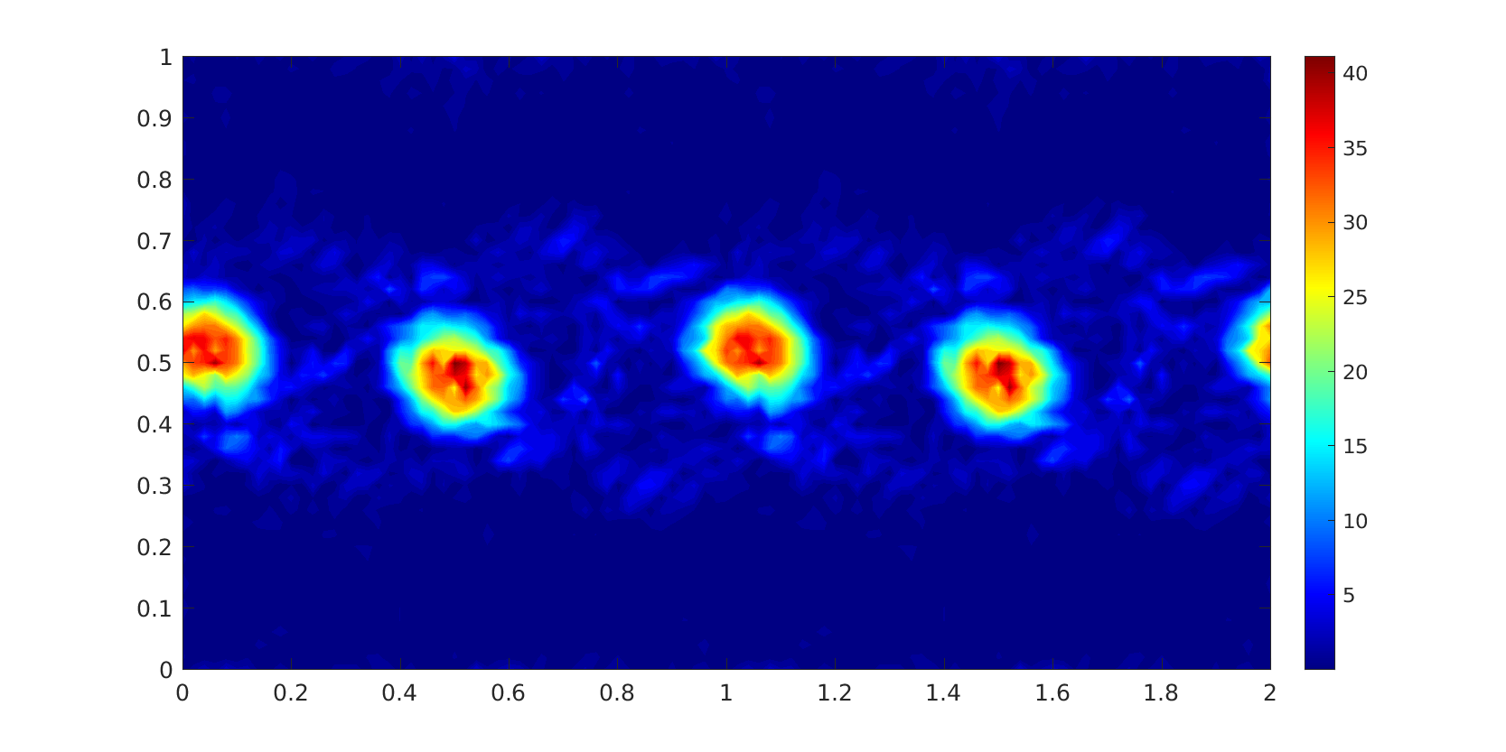


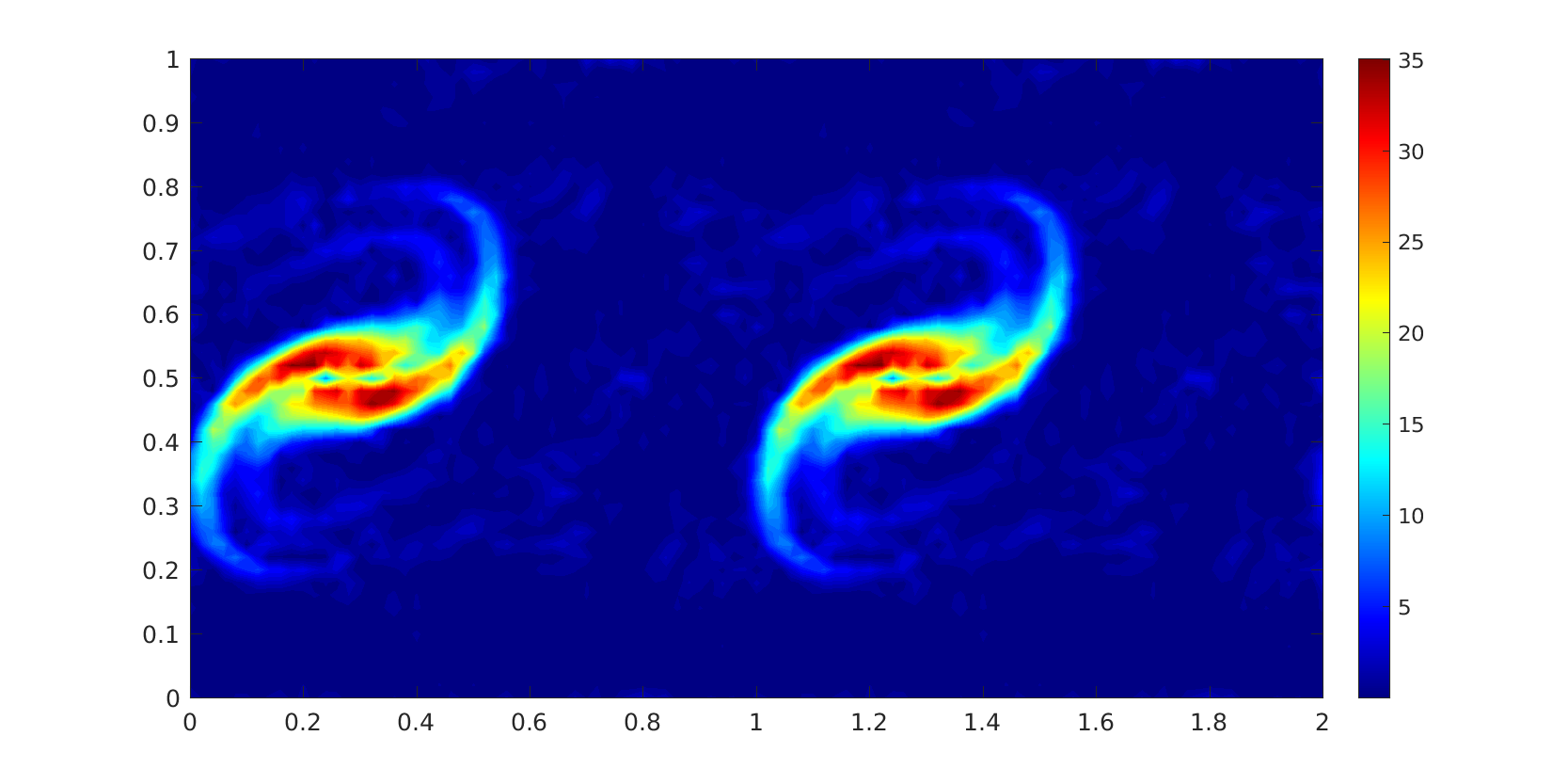


Figure 5 displays enstrophy contours at different times. It was shown in [43] that SKEW does not give resolved plots and show oscillations on a mesh significantly more refined than this one. We can expect that on a coarser mesh that SKEW performs even more poorly, which was made clear during the experiment.
It was also shown in [43] that EMAC performed well on a finer mesh, however on the coarse mesh it does not predict important physical phenomena that happens earlier on in the simulation. Notice at time , EMAC-Reg shows clear vortices, whereas EMAC is more grainy. At times we see a more refined plot from EMAC-Reg of the vortices’ behavior than EMAC.
Comparing to the reference solution, the earlier times for EMAC-Reg closely resemble the resolved solution, much more than EMAC. As mentioned above, we observe several small vortices in the early phases of the experiment for EMAC-Reg, which is precisely how it is depicted in [53]. We also see that EMAC-Reg converges to a steady solution closer to the time where the reference converges. We see convergence begin to form in the reference solution at , whereas EMAC converges around and EMAC-Reg converges around .
5 Conclusions
We have introduced a new regularization model for fluid flow that not only conserves the same important physical quantities as EMAC using a properly chosen time integrator (Crank-Nicolson), but it also performs better than EMAC on coarser meshes. We proved well-posedness of the semidiscrete EMAC-Reg scheme and provided an error analysis that showed optimal rates and a Gronwall constant that does not depend on the Reynold’s number. We also showed numerically that EMAC-Reg outperforms related models on a coarser mesh in terms of error and accuracy over time. Our results show the robustness of regularization models on coarser meshes along with models that conserve important physical quantities.
For future directions, further showing that EMAC-Reg conserves more quantities such as vorticity, enstrophy and helicity would make it more comparable to EMAC. The theoretical analysis of the fully discrete scheme was not included in this paper, this is something that could be shown in a future work. We also only showed that energy, momentum, and angular momentum are only conserved given the proper time integrator. It behooves us to show this for a general case in the future. More numerical testing is also in order, in particular, testing EMAC-Reg in 3D.
Acknowledgments
Clemson University is acknowledged for allowing a generous amount of computation time on the Palmetto cluster.
References
- [1] R.V. Abramov and A.J. Majda. Discrete approximations with additional conserved quantities: deterministic and statistical behavior. Methods Appl. Anal., 10(2):151–190, 2003.
- [2] N. Adams and S. Stolz. A subgrid-scale deconvolution approach for shock capturing. Journal of Computational Physics, 2002.
- [3] N. A. Adams and S. Stolz. On the approximate deconvolution procedure for LES. Physics of Fluids, 2:1699–1701, 1999.
- [4] A. Arakawa. Computational design for long-term numerical integration of the equations of fluid motion: Two dimensional incompressible flow, Part I. J. Comput. Phys., 1:119–143, 1966.
- [5] D. Arndt, W. Bangerth, B. Blais, T. Clevenger, M. Fehling, A. Grayver, T. Heister, L. Heltai, M. Kronbichler, M. Maier, et al. The deal. ii library, version 9.2. Journal of Numerical Mathematics, 1(ahead-of-print), 2020.
- [6] D. Arnold and J. Qin. Quadratic velocity/linear pressure Stokes elements. In R. Vichnevetsky, D. Knight, and G. Richter, editors, Advances in Computer Methods for Partial Differential Equations VII, pages 28–34. IMACS, 1992.
- [7] L.C. Berselli, T. Iliescu, and W.J. Layton. Mathematics of large eddy simulation of turbulent flows. Scientific Computation. Springer-Verlag, Berlin, 2006.
- [8] A. Bowers, T.-Y. Kim, M. Neda, L. Rebholz, and E. Fried. The Leray--deconvolution model: energy analysis and numerical algorithms. Applied Mathematical Modelling, 37(3):1225–1241, 2013.
- [9] S. Breckling, M. Neda, and F. Pahlevani. A sensitivity study of the Navier–Stokes- model. Computers & Mathematics with Applications, 75(2):666–689, 2018.
- [10] T. Chacon-Rebello and R. Lewandowski. Mathematical and numerical foundations of turbulence models and applications. Springer, New York, 2014.
- [11] S. Charnyi, T. Heister, M. Olshanskii, and L. Rebholz. On conservation laws of Navier-Stokes Galerkin discretizations. Journal of Computational Physics, 337:289–308, 2017.
- [12] S. Charnyi, T. Heister, M. Olshanskii, and L. Rebholz. Efficient discretizations for the EMAC formulation of the incompressible Navier-Stokes equations. Applied Numerical Mathematics, 141:220–233, 2019.
- [13] S. Chen, C. Foias, D.D. Holm, E. Olson, E.S. Titi, and S. Wynne. The Camassa–Holm equations as a closure model for turbulent channel and pipe flow. Physical Review Letters, 81:5338–5341, 1998.
- [14] S. Chen, C. Foias, E. Olson, E.S. Titi, and W. Wynne. The Camassa–Holm equations and turbulence. Physica D, 133:49–65, 1999.
- [15] A. Cheskidov, D. Holm, E. Olson, and E.S. Titi. On a Leray- model of turbulence. Proceedings of The Royal Society A, 461:629–649, 2005.
- [16] A. J. Chorin. Numerical solution for the Navier-Stokes equations. Math. Comp., 22:745–762, 1968.
- [17] J. Connors. Convergence analysis and computational testing of the finite element discretization of the Navier–Stokes model. Numerical Methods for Partial Differential Equations, 26(6):1328–1350, 2010.
- [18] V. Cuff, A. Dunca, C. Manica, and L. Rebholz. The reduced order NS- model for incompressible flow: theory, numerical analysis and benchmark testing. ESAIM: Mathematical Modelling and Numerical Analysis, 49(3):641–662, 2015.
- [19] A. Dunca and Y. Epshteyn. On the Stolz-Adams deconvolution model for the large-eddy simulation of turbulent flows. SIAM J. Math. Anal., 37(6):1890–1902, 2005.
- [20] J. A. Evans and T. J. R. Hughes. Isogeometric divergence-conforming B-splines for the steady Navier–Stokes equations. Mathematical Models and Methods in Applied Sciences, 23(08):1421–1478, 2013.
- [21] J. A. Evans and T. J. R. Hughes. Isogeometric divergence-conforming B-splines for the unsteady Navier–Stokes equations. Journal of Computational Physics, 241:141–167, 2013.
- [22] O. Lehmkuhl F. Sacco, B. Paun, T. Iles, P. Iaizzo, G. Houzeaux, M. Vzaquex, C. Butakoff, and J. Aguado-Sierra. Evaluating the roles of detailed endocardial structures on right ventricular haemodynamics by means of CFD simulations. International Journal for Numerical Methods in Biomedical Engineering, 34:1–14, 2018.
- [23] O. Lehmkuhl F. Sacco, B. Paun, T. Iles, P. Iaizzo, G. Houzeaux, M. Vzaquex, C. Butakoff, and J. Aguado-Sierra. Left ventricular trabeculations decrease the wall shear stress and increase the intra-ventricular pressure drop in CFD simulations. Frontiers in Physiology, 9:1–15, 2018.
- [24] G. Fix. Finite element models for ocean circulation problems. SIAM Journal on Applied Mathematics, 29(3):371–387, 1975.
- [25] C. Foias, D.D. Holm, and E.S. Titi. The Navier–Stokes- model of fluid turbulence. Physica D, 152:505–519, 2001.
- [26] C. Foias, D.D. Holm, and E.S. Titi. The three dimensional viscous Camassa–Holm equations, and their relation to the Navier–Stokes equations and turbulence theory. Journal of Dynamics and Differential Equations, 14:1–35, 2002.
- [27] U. Frisch. Turbulence. Cambridge University Press, 1995.
- [28] B.J. Geurts and D. Holm. Regularization modeling for large eddy simulation. Physics of Fluids, 15:L13, 2003.
- [29] B.J. Geurts and D. Holm. Leray and LANS- modeling of turbulent mixing. Journal of Turbulence, 7:1–33, 2006.
- [30] J. Guzman and M. Neilan. Conforming and divergence-free Stokes elements in three dimensions. IMA Journal of Numerical Analysis, 34(4):1489–1508, 2014.
- [31] J. Guzman and M. Neilan. Conforming and divergence-free Stokes elements on general triangular meshes. Mathematics of Computation, 83:15–36, 2014.
- [32] D. Holm and B.T. Nadiga. Modeling mesoscale turbulence in the barotropic double-gyre circulation. Journal of Physical Oceanography, 33:2355–2365, 2003.
- [33] A.N. Kolmogorov. Dissipation of energy in isotropic turbulence. Dokl. Akad. Nauk. SSSR, 32:19–21, 1941.
- [34] A.N. Kolmogorov. The local structure of turbulence in incompressible viscous fluids at very large Reynolds numbers. Dokl. Akad. Nauk. SSSR, 30:299–303, 1941.
- [35] A.N. Kolmogorov. On the degeneration of isotropic turbulence in an incompressible viscous fluids. Dokl. Akad. Nauk. SSSR, 31:538–541, 1941.
- [36] W. Layton. Introduction to the Numerical Analysis of Incompressible Viscous Flows. SIAM, 2008.
- [37] W. Layton. An Introduction to the Numerical Analysis of Viscous Incompressible Flows. SIAM, Philadelphia, 2008.
- [38] W. Layton, C. Manica, M. Neda, and L. Rebholz. Numerical analysis and computational testing of a high accuracy Leray-deconvolution model of turbulence. Numerical Methods for Partial Differential Equations, 24(2):555–582, 2008.
- [39] W. Layton and L. Rebholz. Approximate Deconvolution Models of Turbulence: Analysis, Phenomenology and Numerical Analysis. Springer-Verlag, 2012.
- [40] O. Lehmkuhl, U. Piomelli, and G. Houzeaux. On the extension of the integral length-scale approximation model to complex geometries. International Journal of Heat and Fluid Flow, 78(108422):1–12, 2019.
- [41] J. Liu and W. Wang. Energy and helicity preserving schemes for hydro and magnetohydro-dynamics flows with symmetry. J. Comput. Phys., 200:8–33, 2004.
- [42] R. Martin, M. Soria, O. Lehmkuhl, A. Gorobets, and A. Duben. Noise radiated by an open cavity at low Mach number: Effect of the cavity oscillation mode. International Journal of Aeroacoustics, 18(6-7):647–668, 2019.
- [43] M. Olshanskii and L. Rebholz. Longer time accuracy for incompressible Navier-Stokes simulations with the EMAC formulation. Computer Methods in Applied Mechanics and Engineering, 372:113369, 2020.
- [44] H. Owen, G. Chrysokentis, M. Avila, D. Mira, G. Houzeaux, R. Borrell, J. C. Cajas, and O. Lehmkuhl. Wall-modeled large-eddy simulation in a finite element framework. International Journal for Numerical Methods in Fluids, 92(1):20–37, 2020.
- [45] A. Palha and M. Gerritsma. A mass, energy, enstrophy and vorticity conserving (MEEVC) mimetic spectral element discretization for the 2D incompressible Navier–Stokes equations. Journal of Computational Physics, 328:200–220, 2017.
- [46] D. Pastrana, J.C. Cajas, O. Lehmkuhl, I .Rodríguez, and G. Houzeaux. Large-eddy simulations of the vortex-induced vibration of a low mass ratio two-degree-of-freedom circular cylinder at subcritical Reynolds numbers. Computers and Fluids, 173:118–132, 2018.
- [47] S. Pope. Turbulent Flows. Cambridge University Press, 2000.
- [48] L. Rebholz. An energy and helicity conserving finite element scheme for the Navier-Stokes equations. SIAM Journal on Numerical Analysis, 45(4):1622–1638, 2007.
- [49] L. Rebholz. Conservation laws of turbulence models. Journal of Mathematical Analysis and Applications, 326(1):33–45, 2007.
- [50] L. Rebholz, T.-Y. Kim, and Y.-L. Byon. On an accurate model for coarse mesh turbulent channel flow simulation. Applied Mathematical Modelling, 43:139–154, 2017.
- [51] T. C. Rebollo and R. Lewandowski. Mathematical and numerical foundations of turbulence models and applications. Springer, 2014.
- [52] R. Salmon and L.D. Talley. Generalizations of Arakawa’s Jacobian. J. Comput. Phys., 83:247–259, 1989.
- [53] P. Schroeder, V. John, P. Lederer, C. Lehrenfeld, G. Lube, and J. Schoberl. On reference solutions and the sensitivity of the 2D Kelvin-Helmholtz instability problem. Computers and Mathematics with Applications, 77(4):1010–1028, 2019.
- [54] P. Schroeder and G. Lube. Pressure-robust analysis of divergence-free and conforming FEM for evolutionary incompressible Navier-Stokes flows. Journal of Numerical Mathematics, 25(4):249–276, 2017.
- [55] J. S. Smagorinsky. General circulation experiments with the primitive equations. Mon. Weather Rev., 91:99–164, 1963.
- [56] C. Sorgentone, S. La Cognata, and J. Nordstrom. A new high order energy and enstrophy conserving Arakawa-like Jacobian differential operator. Journal of Computational Physics, 301:167–177, 2015.
- [57] S. Stolz, N. Adams, and L. Kleiser. The approximate deconvolution model for large-eddy simulations of compressible flows and its application to shock-turbulent-boundary-layer interaction. Physics of Fluids, 2001.
- [58] X. Xie, D. Wells, Z. Wang, and T. Iliescu. Numerical analysis of the leray reduced order model. Journal of Computational and Applied Mathematics, 328:12–29, 2018.
- [59] S. Zhang. A new family of stable mixed finite elements for the 3D Stokes equations. Mathematics of Computation, 74:543–554, 2005.
Appendix A Momentum/angular momentum conservation of NS- and Leray- formulations
Here we show that the NS- and Leray- formulations do not conserve momentum or angular momentum if and where represents the filtered velocity . Further note where .
A.1 NS-
Recall the nonlinear term of the NS- formulation is
| (45) |
Test (45) with for . After applying the space-time divergence theorem and rearranging some we get
| (46) |
Assuming , (46) simplifies into
If the nonlinear term is equal to zero, then we will have momentum conservation. We now check this:
where the above two equalities come from vector identities. Also note that because is a vector of scalars, . This leaves us with
which we cannot conclude is zero, hence we cannot say that the NS- formulation preserves momentum.
A.2 Leray-
Recall the nonlinear term of the Leray- formulation is
| (47) |
We test (47) with for and integrate. Similar to (46)
| (48) |
Assuming , (48) simplifies to
If the nonlinear term is equal to zero, then we will have momentum conservation. Using (11) on the nonlinear term we get
which is not zero when . Hence momentum is not necessarily conserved.
For angular momentum we test (47) with for and it simplifies to
Now similarly to the momentum proof, we have for the nonlinear term
where the first term disappears by applying (28) similarly to Theorem 3.3 (and the angular momentum proof for NS- in Appendix A.1). Thus the nonlinear term does not vanish, so angular momentum is not conserved.