Hyperspectral Unmixing via Nonnegative Matrix Factorization with Handcrafted and Learnt PriorsThanks: M. Zhao, T. Gao, J. Chen are with School of Marine Science and Technology, Northwestern Polytechnical University, China. W. Chen is with State Key Laboratory of Rail Traffic Control and Safety, Beijing Jiaotong University, China. (Corresponding author: J. Chen, dr.jie.chen@ieee.org).
Abstract
Nowadays, nonnegative matrix factorization (NMF) based methods have been widely applied to blind spectral unmixing. Introducing proper regularizers to NMF is crucial for mathematically constraining the solutions and physically exploiting spectral and spatial properties of images. Generally, properly handcrafting regularizers and solving the associated complex optimization problem are non-trivial tasks. In our work, we propose an NMF based unmixing framework which jointly uses a handcrafting regularizer and a learnt regularizer from data. we plug learnt priors of abundances where the associated subproblem can be addressed using various image denoisers, and we consider an -norm regularizer to the abundance matrix to promote sparse unmixing results. The proposed framework is flexible and extendable. Both synthetic data and real airborne data are conducted to confirm the effectiveness of our method.
Index Terms:
Hyperspectral unmixing, nonnegative matrix factorization, learnt priors.I Introduction
With the development of remote sensing and hyperspectral sensors, hyperspectral imaging has been widely adopted in many fields. However, due to the low spatial resolution of hyperspectral sensors and the complexity of material mixing process, an observed pixel may contain several different materials. Hyperspectral unmixing analyzes the mixed pixel at a subpixel level, by decomposing the mixed pixel into a set of endmembers and their corresponding fractional abundances [1, 2].
In the past few decades, many hyperspectral unmixing methods have been proposed, including step-by-step unmixing methods (first extracting endmembers and then estimating abundances) and simultaneous decomposing methods (simultaneously determining endmembers and abundances ). Nonnegative matrix factorization (NMF) is a popular simultaneously decomposing method. It represents a hyperspectral image by a product of two nonnegative matrices under the linear mixing assumption, namely, one represents the endmember matrix, and the other represents the abundance matrix [3]. However, NMF is a nonconvex problem that does not admit a unique solution. To overcome this drawback, regularizers are proposed to be added to the objective function to mathematically constrain the space of solutions as well as physically exploit the spatial and spectral properties of hyperspectral images. So far, sparsity and spatial smoothness are the most useful and common regularizers [4, 5]. As mixed pixels often contain a subset of endmembers, sparsity-promoting regularizers have been widely applied in NMF based unmixing methods [6, 7]. The -norm [8], and more generally, -norm () [9, 5] regularizers are introduced to produce sparse unmixing results. Thus, many NMF works use the -norm to enhance the sparsity of results. Spatial smoothness is an inherent characteristic of natural hyperspectral images. Many works integrate the total-variation (TV) regularization to enhance the similarities of neighbor pixels [10, 9]. Reweight TV regularization is also proposed to adaptively capture the smooth structure of abundance maps [8, 11]. Graph based regularization is also a sophisticated choice to cope with spatial information, especially images with complex structures. Many works, such as MLNMF [12], AGMLNMF [13] and SGSNMF [14], use graph regularization to capture the comprehensive spatial information. SSRNMF [15] uses the -norm and the -norm to jointly capture spatial and spectral priors. However, all these methods use handcrafted regularizers to learn the inherent information of hyperspectral data and enhance the unmixing accuracy of NMF. Generally, designing a proper regularization is a non-trivial task, and complex regularizers may increase the difficulty of solving the optimization problem. Several plug-and-play methods have been proposed to solve various hyperspectral image inverse problems [16, 17, 18]. However, this strategy has not been considered in the hyperspectral unmixing with NMF.
In this letter, we propose a novel NMF based unmixing framework which jointly considers both handcrafted and learnt regularizers to fully investigate the prior information embedded in hyperspectral images. To be specific, we plug the learnt spectral and spatial information by using a denoising operator. Using such an operator gets rid of manually designing regularizer and solving the complex optimization problems. A variety of denoisers can be plugged into the framework, which make the method flexible and extendable. Further, handcrafted prior is also kept to encode some physically explicit priors. We add an -norm to the objective function to enhance the sparsity of abundances as an example, as the number of endmembers is usually larger than the number of materials existing in a mixed pixel.
II Problem Formulation
We consider the linear mixture model (LMM), which assumes that an observed pixel is a linear combination of a set of endmembers and their associated fractional abundances. Let be an observed hyperspectral image, where is the number of spectral bands, is the number of pixels. The LMM for a hyperspectral image can be expressed as:
| (1) |
where is an matrix, which denotes the endmember spectra library with the number of endmembers, and is a matrix representing the abundance matrix, and denotes an i.i.d. zero-mean Gaussian noise matrix. For the physical characteristics of hyperspectral data, the endmember matrix is required to satisfy the endmember nonnegative constraint (ENC), and the abundance matrix is required to satisfy the abundance nonnegative constraint (ANC) and sum-to-one constraint (ASC), i.e., and .
III Proposed Method
In our work, we propose an NMF based unmixing framework which uses a handcrafted regularizer and learnt priors to enhance the unmixing performance. More specially, we use an -norm to enhance the sparsity of abundances, and we plug the learnt spectral and spatial information by using a denoising operator. We shall elaborate our framework as follows.
III-A Objective Function
We use the NMF model to solve the blind unmixing problem. The general objective function is expressed as:
| (2) |
The terms on the right-hand-side of (2) are interpreted as follows:
- •
is the term associated with the data fitting quality. In this work, we set , with being the Frobenius norm.
- •
is a regularization term that represents priors learnt from data, which does not has an explicit form. Here we only concentrate on priors of by setting for illustration purpose.
- •
is a handcrafted regularization term. Though the learnt regularizer is powerful to represent spatial-spectral information of the image, is still necessary to encode physically meaningful properties and the prior knowledge of endmebers that might not easy to be learnt. Here, we use , which is a structured sparsity regularizer showing effectiveness in sparse unmixing. Other meaningful handcrafted regularization can also be adopted.
- •
is a positive parameter that controls the impact of the sparse regularizer. The positive regularization parameter controls the strength of plugged priors.
Then, the unmixing problem writes:
| (3) |
where , and is the -th row of . The same as some previous works [8, 10], we introduce an auxiliary variable and constraint . The objective function (3) is rewritten as:
| (4) |
The associated augmented Lagrangian function is given by
| (5) |
where is the penalty parameter. The blind unmixing problem can be solved by iteratively addressing the following three subproblems:
| (6) | ||||
| (7) | ||||
| (8) |
The first two subproblems are forward models used to update the endmember and abundance matrices. We use the NMF method to solve the first two subproblems. As to be seen later, the third subproblem can be considered as an image denoising problem which can be solved by a variety of denoisers. This framework is flexible and can automatically plug spatial and spectral priors with the choice of different denoisers.
III-B Optimization
III-B1 Endmember estimation
In order to estimate the endmember matrix, we devote to solve the following minimization objective problem:
| (9) |
where is the Lagrange multiplier to control the impact of ENC. We calculate the gradients about and set it to :
| (10) |
By element-wise multiplication of both sides of (10) and according to the Karush-Kuhn-Tucker (K-K-T) conditions , the endmember matrix is updated as:
| (11) |
where is element-wise multiplication, and is element-wise division.
III-B2 Abundance estimation
The second subproblem is to estimate abundance. It is difficult to solve ASC, and we use two augmented matrixes to address this issue:
| (12) |
where is the penalty parameter controlling the strength of ASC. The objective problem of abundance estimation is as follows:
| (13) |
where is the Lagrange multiplier to control the impact of ANC. We calculate the derivative of (13) and set it to 0:
| (14) |
where
| (15) |
According to KKT conditions, we get . By element-wise multiplication of both sides of (14), we update the abundance matrix as follows:
| (16) |
III-B3 Plugged priors
In the third subproblem, we focus on solving the following optimization problem:
| (17) |
This step can be seen as an abundance denoising problem, where is the clean version of abundance maps. This problem can be rewritten as:
| (18) |
According to the maximum a posteriori model (MAP), the problem in (18) can be regarded as denoising abundance maps with additive gaussian noise with a standard deviation and the priors are encoded in . In our proposed unmixing framework, instead of solving this problem using optimization methods, we use denoisers to solve this regularized optimization problem. Plugged denoisers can automatically carry prior information. The denoising operator is actually performed in the 3D domain to fully exploit the spectral and spatial information, we rewrite (18) as follows:
| (19) |
where is an operator that transforms the 2D matrix to 3D data cube. Plenty of denoisers can be applied in this step and carry various kinds of priors. In our work, we use a conventional linear denoiser non-local means denoising (NLM), a nonlinear denoiser block-matching and 3D filtering (BM3D) to our NMF based unmixing framework. These two denoisers are 2D cube based and solve the abundances denoising problem band by band. Further, two 3D cube based denoisers BM4D and a total variation regularized low-rank tensor decomposition denoising model (LRTDTV) are also plugged into our proposed framework. We denote our proposed methods as PNMF-NLM, PNMF-BM3D, PNMF-BM4D and PNMF-LRTDTV, respectively. Our NMF based unmixing framework is presented in Algorithm 1.
while Stopping criterias are not met and do 1
Augment and to obtain and , respectively;
Update with (16);
Update using the strategy of (19);
; end while 2
IV Experiments
| 5dB | 10dB | 20dB | 30dB | |||||||||
| RMSE | SAD | PSNR | RMSE | SAD | PSNR | RMSE | SAD | PSNR | RMSE | SAD | PSNR | |
| VCA-SUnSAL-TV | 0.1392 | 6.0675 | 17.5317 | 0.0692 | 3.0419 | 23.1989 | 0.0240 | 0.7611 | 32.4014 | 0.0094 | 0.1880 | 40.5592 |
| CoNMF | 0.1074 | 6.8326 | 9.7881 | 0.0773 | 4.4600 | 22.2385 | 0.0248 | 0.7609 | 32.1133 | 0.0094 | 0.1879 | 40.5005 |
| TV-RSNMF | 0.1390 | 6.0034 | 9.6711 | 0.0740 | 4.3929 | 22.6155 | 0.0265 | 1.0429 | 31.5214 | 0.0092 | 0.2169 | 40.7600 |
| NMF-QMV | 0.1392 | 23.4638 | 17.1248 | 0.0854 | 8.3570 | 21.3688 | 0.0247 | 0.6208 | 32.1312 | 0.0092 | 0.1902 | 40.6972 |
| PNMF-NLM | 0.0817 | 5.1458 | 22.2549 | 0.0560 | 2.9961 | 24.8780 | 0.0212 | 0.5116 | 33.0728 | 0.0092 | 0.1877 | 40.1695 |
| PNMF-BM3D | 0.0779 | 5.1164 | 23.4658 | 0.0557 | 2.0428 | 25.2735 | 0.0176 | 0.3898 | 35.2867 | 0.0092 | 0.1878 | 40.5740 |
| PNMF-BM4D | 0.0838 | 5.2499 | 21.2835 | 0.0579 | 2.0840 | 25.4650 | 0.0186 | 0.4242 | 34.4498 | 0.0092 | 0.1876 | 41.0646 |
| PNMF-LRTDTV | 0.0773 | 5.0415 | 21.9143 | 0.0597 | 2.7060 | 25.1639 | 0.0211 | 0.4873 | 33.5669 | 0.0091 | 0.1878 | 40.5740 |
In this section, we use both synthetic data and real data experiments to evaluate the unmixing performance of our proposed NMF based unmixing framework. Our methods were compared with several state-of-the-art methods. First, we considered a sequential unmixing method, where we extracted the endmembers with VCA [19] and estimated the abundances using SUnSAL-TV [20]. We also compared with NMF based methods. CoNMF [3] is a robust collaborative NMF method for hyperspectral unmixing. TV-RSNMF [8] is a TV regularized reweighted sparse NMF method. NMF-QMV [21] is a variational minimum volume regularized NMF method. We used the spectral angle distance (SAD) to evaluate the endmember extraction results: where is the ground-truth and is the estimated endmember. We used the root mean square error (RMSE) to evaluate the abundance estimation results: where is the -th column of and represents the ground-truth, and is the estimated abundance. Further, we used the peak signal-to-noise ratio (PSNR) to evaluate the denoising quality between estimated abundances and ground-truth: in which MAX is the maximum abundance value, and , where is the estimated abundance and is the clean ground-truth.
IV-A Synthetic data
In this experiment, we generated the synthetic data using Hyperspectral Imagery Synthesis tools with Gaussian Fields11 1 http://www.ehu.es/ccwintco/index.php/Hyperspectral_Imagery_Synthesis_ tools_for_MATLAB, and the LMM is adopted. The spatial size of the synthetic data is . A selection of four endmembers from USGS spectral library were used as the endmember library, with bands covering wavelength from 400 nm to 2500 nm. There are both mixed and pure pixels in the dataset. To evaluate the robustness of our methods and the efficacy of plugged denoisers, we added Gaussian noise to the clean data with the signal-to-noise ratio (SNR) setting to 5 dB, 10 dB, 20 dB and 30 dB.
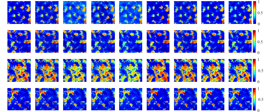
In our work, we used VCA to initialize the endmembers and the fully constrained least square method (FCLS) [22] to initialize the abundances. After multiple experiments, we set the penalty parameter of () to 0.1, the penalty parameter of denoising term () to , the penalty parameter of ASC () to 10, and to 500. Unmixing results of RMSE, SAD and PSNR of this experiment are reported in Table I. From the results, we observe that our proposed methods get the best RMSE and PSNR results and achieve the lowest mean SAD values than other methods. This highlights the effects of our sparse regularizer and the superiority of priors learnt by denoisers. Moreover, benefitting from the denoisers, when the noise level is high, the unmixing results of our methods show more significant enhancement. This indicates that our methods are robust to noise. Figure 1 shows the abundance maps of four compared methods and our proposed methods with SNR = 10 dB. We can see that the abundance estimated results of our methods are with less noise and more close to ground-truth. The endmember extracted results of PNMF-NLM (SNR = 20 dB) are shown in Figure 2, where the red curves are ground-truth, and the blue curves are estimated endmembers. Moreover, Figure 3 presents how parameters affect the unmixing results with SNR = 10 dB. The RMSE convergence curves of synthetic data of our proposed methods are shown in Figure 4, which indicate that our NMF based unmixing framework has a stable convergence property.
IV-B Real data
IV-B1 Cuprite dataset
In this experiment, we used a well-known real hyperspectral dataset (AVIRIS Cuprite) to evaluate our unmixing methods. The dataset was captured from the Cuprite mining district in west-central Nevada by AVIRIS in 1997. We used a subimage of size in our experiment. This dataset has bands. Following other works [3, 13], we removed the water absorption and noisy bands (2, 105-115, 150-170, 223 and 224) with 188 exploitable bands remained. The number of endmembers was set to 12.
In this experiment, we set to 0.1, to , to 10 and to 100. As there is no ground-truth for this dataset, we can not give a quantitative comparison. Like many previous works, we evaluate the unmixing results in an intuitive manner. The abundance maps of selected materials of the Cuprite data are shown in Figure 6. We observe that our proposed methods provide clearer and sharper results with several locations emphasized and more detailed information. The endmember extraction results of PNMF-BM4D are shown in Figure 5. We also used reconstructed error (RE) to qualify these methods: where represents the reconstructed pixel, and is the ground-truth. The RE comparison is shown in Table II. We observe that PNMF-BM4D gets the lowest RE results. Note that without the ground-truth information on the abundances and endmembers for the real data, RE is not necessarily proportional to the quality of unmixing performance, and therefore it can only be considered as complementary information. Note that our methods use denoisers to plug learnt priors, which can also denoise the abundance maps but may increase the RE compared to the noisy input.

| Algorithm | VCA-SUnSAL-TV | CoNMF | TV-RSNMF | NMF-QMV | PNMF-NLM | PNMF-BM3D | PNMF-BM4D | PNML-LRTDTV |
| RE | 0.0087 | 0.0235 | 0.0085 | 0.0425 | 0.0083 | 0.0081 | 0.0070 | 0.0091 |
IV-B2 Jasper Ridge dataset
The Jasper Ridge dataset with pixels was used for this purpose. The data consist of 224 spectral bands ranging from 380 nm to 2500 nm with spectral resolution up to 10 nm. After removing channels [1-3, 108-112, 154-166 and 220-224] affected by dense water vapor and the atmosphere, 198 channels were remained. Four prominent endmembers existing in this data are considered in our experiments.
The experiment settings are the same as Cuprite dataset. We set to 0.1, to , to 10 and to 100. The abundance estimated results are shown in Figure 7, and the endmembers extracted from PNMF-BM4D is shown in 8. The unmixing results indicate that our proposed methods are with less noise and more smoothness. RE results of Jasper Ridge dataset are shown in Table III, which also demonstrate the effective performance of our methods.

| Algorithm | VCA-SUnSAL-TV | CoNMF | TV-RSNMF | NMF-QMV | PNMF-NLM | PNMF-BM3D | PNMF-BM4D | PNML-LRTDTV |
| RE | 0.0257 | 0.0198 | 0.0122 | 0.0434 | 0.0111 | 0.0123 | 0.0135 | 0.0117 |
V Conclusion
In this paper, we proposed an NMF based unmixing framework that jointly used handcrafted and learnt regularizers. We used a denoiser of abundances to plug learnt priors. Our framework allowed plugging various denoisers which is flexible and extendable. For illustrating the integration of handcrafted regularization, we added a structured sparse regularizer to the objective function to enhance the sparsity of unmixing results. Experiment results showed the effectiveness of our proposed methods. Future work will focus on the adaptive parameter selection.
References
- [1] N. Keshava and J. F. Mustard, “Spectral unmixing,” IEEE Signal Process. Mag., vol. 19, no. 1, pp. 44–57, 2002.
- [2] J. M. Bioucas-Dias, A. Plaza, N. Dobigeon, M. Parente, Q. Du, P. Gader, and J. Chanussot, “Hyperspectral unmixing overview: Geometrical, statistical, and sparse regression-based approaches,” IEEE J. Sel. Top. Appl. Earth Observat. Remote Sens., vol. 5, no. 2, pp. 354–379, 2012.
- [3] J. Li, J. M. Bioucas-Dias, A. Plaza, and L. Liu, “Robust collaborative nonnegative matrix factorization for hyperspectral unmixing,” IEEE Trans. Geosci. Remote Sens., vol. 54, no. 10, pp. 6076–6090, 2016.
- [4] X. Lu, H. Wu, and Y. Yuan, “Double constrained nmf for hyperspectral unmixing,” IEEE Trans. Geosci. Remote Sens., vol. 52, no. 5, pp. 2746–2758, 2013.
- [5] Y. E. Salehani and S. Gazor, “Smooth and sparse regularization for nmf hyperspectral unmixing,” IEEE J. Sel. Top. Appl. Earth Observat. Remote Sens., vol. 10, no. 8, pp. 3677–3692, 2017.
- [6] W. Wang, Y. Qian, and Y. Tang, “Hypergraph-regularized sparse nmf for hyperspectral unmixing,” IEEE J. Sel. Top. Appl. Earth Observat. Remote Sens., vol. 9, no. 2, pp. 681–694, 2016.
- [7] X. Lu, L. Dong, and Y. Yuan, “Subspace clustering constrained sparse nmf for hyperspectral unmixing,” IEEE Trans. Geosci. Remote Sens., 2019.
- [8] W. He, H. Zhang, and L. Zhang, “Total variation regularized reweighted sparse nonnegative matrix factorization for hyperspectral unmixing,” IEEE Trans. Geosci. Remote Sens., vol. 55, no. 7, pp. 3909–3921, 2017.
- [9] J. Sigurdsson, M. O. Ulfarsson, and J. R. Sveinsson, “Blind hyperspectral unmixing using total variation and sparse regularization,” IEEE Trans. Geosci. Remote Sens., vol. 54, no. 11, pp. 6371–6384, 2016.
- [10] X. Feng, H. Li, J. Li, Q. Du, A. Plaza, and W. Emery, “Hyperspectral unmixing using sparsity-constrained deep nonnegative matrix factorization with total variation,” IEEE Trans. Geosci. Remote Sens., vol. 56, no. 10, pp. 6245–6257, 2018.
- [11] X. Feng, H. Li, and R. Wang, “Hyperspectral unmixing based on sparsity-constrained nonnegative matrix factorization with adaptive total variation,” in IGARSS 2019-2019 IEEE International Geoscience and Remote Sensing Symposium. IEEE, 2019, pp. 2139–2142.
- [12] Z. Shu, J. Zhou, L. Tong, X. Bai, and C. Zhao, “Multilayer manifold and sparsity constrainted nonnegative matrix factorization for hyperspectral unmixing,” in 2015 IEEE International Conference on Image Processing (ICIP). IEEE, 2015, pp. 2174–2178.
- [13] L. Tong, J. Zhou, B. Qian, J. Yu, and C. Xiao, “Adaptive graph regularized multilayer nonnegative matrix factorization for hyperspectral unmixing,” IEEE J. Sel. Top. Appl. Earth Observat. Remote Sens., vol. 13, pp. 434–447, 2020.
- [14] X. Wang, Y. Zhong, L. Zhang, and Y. Xu, “Spatial group sparsity regularized nonnegative matrix factorization for hyperspectral unmixing,” IEEE Trans. Geosci. Remote Sens., vol. 55, no. 11, pp. 6287–6304, 2017.
- [15] R. Huang, X. Li, and L. Zhao, “Spectral–spatial robust nonnegative matrix factorization for hyperspectral unmixing,” IEEE Trans. Geosci. Remote Sens., vol. 57, no. 10, pp. 8235–8254, 2019.
- [16] S. Sreehari, S. V. Venkatakrishnan, B. Wohlberg, G. T. Buzzard, L. F. Drummy, J. P. Simmons, and C. A. Bouman, “Plug-and-play priors for bright field electron tomography and sparse interpolation,” IEEE Trans. on Comput. Imaging, vol. 2, no. 4, pp. 408–423, 2016.
- [17] A. M. Teodoro, J. M. Bioucas-Dias, and M. A. Figueiredo, “A convergent image fusion algorithm using scene-adapted gaussian-mixture-based denoising,” IEEE Trans. Image Process., vol. 28, no. 1, pp. 451–463, 2018.
- [18] X. Wang, J. Chen, C. Richard, and D. Brie, “Learning spectral-spatial prior via 3ddncnn for hyperspectral image deconvolution,” in Proc. IEEE Int. Conf. Acoust., Speech, Signal Process. (ICASSP), 2020. IEEE, 2020, pp. 2403–2407.
- [19] J. M. P. Nascimento and J. M. B. Dias, “Vertex component analysis: A fast algorithm to extract endmembers spectra from hyperspectral data,” in Pattern Recognition and Image Analysis, First Iberian Conference, IbPRIA 2003, Puerto de Andratx, Mallorca, Spain, June 4-6, 2003, Proceedings, 2003.
- [20] M. Iordache, J. M. Bioucas-Dias, and A. Plaza, “Total variation spatial regularization for sparse hyperspectral unmixing,” IEEE Trans. Geosci. Remote Sens., vol. 50, no. 11, pp. 4484–4502, 2012.
- [21] L. Zhuang, L. C., F. M. A. T., and J. M. Bioucas-Dias, “Regularization parameter selection in minimum volume hyperspectral unmixing,” IEEE Trans. Geosci. Remote Sens., vol. PP, no. 99, pp. 1–20, 2019.
- [22] D. C. Heinz et al., “Fully constrained least squares linear spectral mixture analysis method for material quantification in hyperspectral imagery,” IEEE Trans. Geosci. Remote Sens., vol. 39, no. 3, pp. 529–545, 2001.