MIMO ILC for Precision SEA Robots using Input-Weighted Complex-Kernel Regressionfootnoteinfo
Abstract
This work improves the positioning precision of lightweight robots with series elastic actuators (SEAs). Lightweight SEA robots, along with low-impedance control, can maneuver without causing damage in uncertain, confined spaces such as inside an aircraft wing during aircraft assembly. Nevertheless, substantial modeling uncertainties in SEA robots reduce the precision achieved by model-based approaches such as inversion-based feedforward. Therefore, this article improves the precision of SEA robots around specified operating points, through a multi-input multi-output (MIMO), iterative learning control (ILC) approach. The main contributions of this article are to (i) introduce an input-weighted complex kernel to estimate local MIMO models using complex Gaussian process regression (c-GPR) (ii) develop Geršgorin-theorem-based conditions on the iteration gains for ensuring ILC convergence to precision within noise-related limits, even with errors in the estimated model; and (iii) demonstrate precision positioning with an experimental SEA robot. Comparative experimental results, with and without ILC, show around % improvement in the positioning precision (close to the repeatability limit of the robot) and a -times increase in the SEA robot’s operating speed with the use of the MIMO ILC.
keywords
Inversion; Iterative methods; Learning control; Non-parametric regression; Robot controlfootnoteinfo]This research was conducted in the Mechanical Engineering Department at the University of Washington.
, , , , ,
1 Introduction
Lightweight, relatively-small, SEA robots are well suited for automating manufacturing tasks in confined spaces such as an aircraft wing or tail, e.g., for cleaning pilot holes (used for fixtures) during aircraft assembly. Often these are hard to reach spaces, and workers need to crawl through tight spaces and manual operations can be ergonomically challenging. The robot needs to be lightweight (around 20 pounds or less) for easy placement, often by hand. Moreover, direct estimates of the joint forces found by measuring the deformation of the elastic element in SEAs [1], along with low-impedance control can limit the forces applied by the robot when maneuvering under uncertainty in confined spaces, which can help avoid potential damage to the workpiece and costly repairs. Nevertheless, this increased control over forces during maneuvering in uncertain environments comes at the cost of lower positioning precision of lightweight robots [2], even at the final operating points where the environmental uncertainty might be lower. However, precision positioning, around an operating point is desirable since it can enable the use of lightweight SEA robots in manufacturing tasks in hard-to-reach, confined spaces. Such precision in conjunction with compliance (which avoids damage) can be especially beneficial for contact-type applications such as cleaning of holes. The problem in achieving precision is that the flexural systems in lightweight SEA robots result in non-minimum phase dynamics, and high gains (for improved performance) can lead to instability. Therefore, there are limits to the achievable precision with feedback [3]. In general, model-based methods, such as inversion to find feedforward inputs to augment the feedback, can be used to improve performance of robots, e.g., [4]. A challenge to accurate modeling is the difficulty in capturing nonlinearities and contact-related effects in SEA robots, e.g., [5]. Therefore, tracking error with such model-inversion-based approaches can be large if there are significant model estimation errors. This motivates the current work to improve precision-positioning of SEA robots at different operating points (around which the dynamics can be linearzied), even in the presence of modeling uncertainties. While the current approach is shown to be well suited to improve precision around an operating point, it is not suited for applications where large robot motions are required. In such cases, the nonlinearity can be significant and alternative approaches such as Lyapunov-based iterative methods [6] or iterative methods for model-based impedance control [7] could be considered. Moreover, when the signals are periodic and band-limited, the frequency-domain regression method developed in the current article could be extended to the nonlinear case using generalized frequency-response functions as in [8].
Iterative learning methods can enable precision control even in the presence of modeling uncertainties, especially when the task can be learned ahead of time or can be repeated [9]. Moreover, previously learned precision sub-tasks could be recombined to form new tasks [10]. When the model uncertainty is low, model inversion can be used to improve the performance of robots with elastic joints, e.g., [11] and can be applied to correct for nonminimum-phase flexural dynamics of lightweight robots [12]. Therefore, in this article, a model-inversion-based ILC [13, 14, 15] is used to account for modeling uncertainties with the lightweight SEA robot. However, the ILC iterations could potentially diverge if the modeling uncertainty is large, e.g., [16]. This motivates approaches developed to reduce the model uncertainty to improve convergence [17], by using observed input-output data ( at frequency ) of the form for single-input single-output (SISO) systems, rather than using the inverse of a known model. Even with the direct use of input-output data, the effective model uncertainty can be large still if the signal to noise ratio is small, e.g., when the desired output at some frequency is small [18]. An approach is to not iterate at those specific frequencies where the desired output is small, e.g., [17, 19]. Another approach is to inject additional input at such frequencies (where the desired output is small) to ensure persistence of excitation when estimating the model from data, which enables the learned model to be portable and applicable to track new trajectories, e.g., [20]. In either case, provided the uncertainty is sufficiently small, the ILC converges to the input needed for exact output tracking for SISO systems, even in the presence of modeling uncertainties. Therefore, it is expected that the model-inversion-based ILC approach could improve the precision for the MIMO case, in the presence of small uncertainties, e.g., with the use of a linearized model of the SEA robot obtained at an operating point.
While convergence conditions have been well established for the SISO inversion-based ILC [15], extension to the MIMO inversion-based ILC remains challenging. For sufficiently-diagonally-dominant systems, convergence can be established with the use of a diagonalized inverse model in the ILC as shown in [21]. Recent efforts [22, 24] have considered ILC with the full MIMO inverse [14]. For example, the ILC gain could be optimized to minimize the tracking error with the constraint that the iterations converge, e.g., by using a Q-filter when computing the ILC input [24]. The Q-filter approach trades off between robustness and performance; if the anticipated uncertainty is small, then the tracking error is small, but not zero, when the Q-filter is nontrivial, i.e., . In contrast, this article develops conditions on the ILC gain, using the Geršgorin theorem as in [22], for ensuring convergence to the desired output, even under modeling uncertainty.
A challenge with inversion-based ILC is that the actual system dynamics and the uncertainty are unknown. Therefore, it is difficult to ensure that the convergence condition on the model uncertainty is met. One approach is to use a relatively large number of repetitive experiments for identifying both the model and the uncertainty prior to applying the ILC [15, 24]. An alternative approach is to use kernel-based regression approaches to estimate the model and its uncertainty for the SISO case [20] from data obtained from a relatively-sparse number (one or two) of the ILC iterations. This use of ILC data allows the data-based model to capture the local, linear model near the work area that includes potential contact-dependent effects, which can be challenging to model from first principles. Note that kernel-based Gaussian process regression (GPR, popularly also referred to as machine learning) is well suited to estimation of the general functions (such as the frequency response function) as well as their uncertainty from noisy experimental data [25]. Though complex kernels have been used in the past for GPR [26], they cannot be used to estimate models for multi-input systems. This motivates the development, in the current article, of an input-weighted complex kernel to estimate the complex-valued system MIMO model as well as its uncertainty . Since it is designed in the Fourier domain, it captures the noncausality needed for many system inversion approaches, e.g., as investigated in [27], and can be used with SISO frequency-domain kernels which ensure BIBO stability of the resulting models, e.g., as in [28]. Such kernel-based methods tend to be robust than typical model-identification methods in infinite-dimensional spaces, e.g., as discussed in [29].
The current work extends preliminary results in [22] by (i) proving the conditions for convergence, (ii) using augmented inputs in the ILC to ensure sufficiently large signal-to-noise ratio in the frequency range of interest, and (iii) applying and evaluating the approach for precision control of a lightweight SEA robot. Comparative experimental results, with and without ILC, are presented that show around % improvement in the positioning precision with the use of the MIMO ILC (close to the repeatability limit of the robot) and a -times increase in the SEA robot’s operating speed.
2 Problem Formulation
2.1 Inversion-based iterative-learning control (ILC)
Given a linear time-invariant (LTI) system with transfer function (or frequency response function)
| (1) |
with output and input represented in the Fourier domain at frequency , the goal is to find an input that yields exact tracking of the desired output , i.e.,
| (2) |
where the system is stable and the number of outputs is not more than the number of inputs , i.e., .
Assumption 1
The LTI system has full row rank on the imaginary axis.
Remark 1
The rank condition implies that there are no transmission zeros on the imaginary axis, which guarantees the existence of a finite input that achieves exact tracking of the desired output and ensures robustness of the inverse [30]. However, conditions have been studied recently on when such zeros are acceptable for inversion [31].
The iterative approach generates a new input for use at iteration step based on the tracking error
| (3) |
from the prior iteration step , which is similar to prior use for the square system case, e.g., in [15, 14, 22]
| (4) |
where is the pseudo-inverse of the estimated model of the unknown system with and the identity matrix is denoted by . The superscript denotes the complex conjugate, is an invertible diagonal matrix, with , and is a diagonal matrix with nonnegative elements representing the iteration gain.
Remark 2
For square systems with the same number of inputs and outputs , i.e., , the pseudo-inverse becomes the exact inverse . For the actuator redundant case, i.e., , solves the input-output equation while minimizing the frequency-weighted input cost .
Multiplying on both sides of Eq (4) results in
Subtracting the desired output from both sides yields a relation between error defined in Eq. (3) at consecutive iteration steps, as
| (5) |
where the unknown model uncertainty
| (6) |
In the following, the initial iteration input is selected as the desired output, , which is assumed to be sufficiently smooth and bounded over the frequency range.
Remark 3
The model uncertainty in Eq. (6) quantifies the error in the estimated model , or equivalently the error in computing the pseudo-inverse .
Remark 4
From Assumption 1, the estimated model has full row rank on the imaginary axis for sufficiently small model estimation error .
2.2 Problem statement
The iterations result in a contraction if the model uncertainty is sufficiently small. From Eq. (5), the tracking error , and therefore, with increasing iterations, the tracking error tends to zero in the 2-norm, if and only if , which in turn occurs if and only if the spectral radius of the contraction gain is less than one as in Eq. (9), e.g., see Theorem 5.6.12 in [32]. Therefore, as shown in the previous works e.g., [15, 14, 22], the MIMO ILC in Eq. (4) converges at frequency for any general output , i.e., the tracking error tends to zero
| (7) |
as iterations increase, , if and only if the spectral radius (maximum magnitude of the eigenvalues ) of the the contraction gain
| (8) |
is less than one, i.e.,
| (9) |
Remark 5
Convergence of the tracking error to zero in the two norm also results in convergence in any other norm, since all norms are equivalent in finite-dimensional linear vector spaces, and for any norm there exists a constant such that [32] .
The research issue is to develop conditions on the iteration gain to ensure convergence of the ILC under given bounds on the model uncertainty . This can be split into a model and uncertainty estimation problem and the problem of selecting the iteration gain to ensure convergence.
3 Solution: ILC design for convergence
3.1 Model and uncertainty estimation
The goal is to estimate the model terms from observation given by
| (10) |
where is the measurement noise and system components are replaced by Gaussian Processes due to noise as in previous works, e.g., [28, 29].
If only one input, say , is nonzero, then the system component is a complex function that can be estimated using Gaussian Process Regression (GPR) with previously-developed complex kernels, e.g., the one in [28, 26, 23]. However, such an approach requires separate experiments with only one nonzero input in each experiment, which might not be feasible in general. Such approaches are not directly applicable to the multi-input case.
Towards model identification for the multiple-input case, given any set of complex kernels for , the following input-weighted kernel is proposed for the composite Gaussian process in Eq. (10),
| (11) |
where the subscripts refer to different frequencies belonging to the observed frequency set
| (12) |
with nonzero accompanying input . A motivation for the proposed kernel is that for the single-input case (), using the input-weighted kernel to estimate the component is equivalent to obtaining an estimate with the unweighted kernel based on observed ratios , as shown in Lemma 3 in the following. Moreover, is a valid kernel (Hermetian positive semi-definite) provided the underlying kernels associated with each term are valid kernels, as shown in the lemma below under the following assumption.
Assumption 2
All the complex Gaussian Processes are independent, and have zero-mean prior. Moreover they are assumed to (i) be proper as in [33, 26], resulting in kernel functions that have the same variance for the real and imaginary parts at each frequency ; and (ii) have independent real and imaginary components resulting in .
Lemma 1
With nonzero input at each frequency in the observed frequency set , the input-weighted kernel in Eq. (11) is Hermitian positive semi-definite if the kernels are Hermitian positive semi-definite. Moreover, the self covariance matrix in Eq. (13), associated with , is positive definite if covariance matrices are positive definite for .
PROOF.
The Hermetian property of the input-weighted kernel follows from Eq. (11) since
and positive semi-definiteness follows since each term in the summation in Eq. (11) is non-negative. The covariance can be written as, due to independence of terms from Assumption 2,
| (13) |
The row and column element of the covariance matrix is the evaluation of the input-weighted kernel on frequency-input pair and , which is computed as the input-weighted summation of the corresponding row and column element of each covariance matrix computed as . For any vector ,
where is nonzero if is nonzero. Thus, is positive (semi-) definite if for all , is positive (semi-) definite. ∎
Lemma 2 (Multi-input system identification)
The estimate of each term in Eq. (10) is given by
| (14) |
with estimated variance given by
| (15) |
where is the noise variance at output, is an -by-1 vector with one in the component and zero elsewhere, and
| (16) |
PROOF.
Lemma 3
For SISO case, the estimate of and its variance at any frequency with the original kernel based on ratios are the same as those obtained with input-weighted kernel based on , i.e.,
| (17) | ||||
| (18) |
PROOF.
When , the covariance matrices in Eq. (16) with the input-weighted kernel can be related to the covariance matrices associated with the original kernel based on Eq. (11) and (13), as
| (19) |
with and . Furthermore, the general error covariance matrix for error in Eq. (10) is given by
| (20) |
where is the error covariance matrix of the noise in
| (21) |
because by compraing Eq. (21) and the case of Eq. (10) when , which can be written as below,
| (22) |
the variance relation between the and can be obtained as
| (23) |
Then, substituting Eqs. (19) and (20) into equations to generate the estimation of and using from Eq. (21) results in
which results in the equivalence claim in the lemma. ∎
Remark 6
Lemma 4
Each component of the model uncertainty defined in Eq. (6) is bounded as
| (25) |
PROOF.
This follows by replacing in Eq. (6) by . ∎
3.2 Convergence conditions for MIMO ILC
Lemma 5 (MIMO ILC convergence conditions)
Let each component of the uncertainty in Eq. (6) have the form
| (26) |
with magnitude and phase where . Also let the iteration gain in Eq. (4) be diagonal, i.e., . Then, the MIMO ILC in Eq. (4) converges at frequency if, for all ,
| (27) | ||||
| (28) | ||||
| (29) | ||||
| where | (30) |
PROOF.
The conditions of this lemma are used to show that the eigenvalues of the contraction gain have magnitude less than one, and therefore, the MIMO ILC convergence condition in Eq. (9) is met. By the Geršgorin theorem [32], all the eigenvalues of the contraction gain are in the union of Geršgorin discs centered at with radius . Then, the eigenvalues of the contraction gain are less than one if all the Geršgorin discs are bounded by the unit circle centered at the origin, i.e.,
| (31) |
which can be rewritten using Eq. (8) as
| (32) |
Since the left hand side (LHS) of Eq. (32) is nonnegative, and needs to be strictly less than the right hand side (RHS), the RHS is required to be positive, which is satisfied due to the condition in Eq. (29) and being positive from Eq. (28). Since both sides of Eq. (32) are nonnegative, squaring them and using Eq. (26) results in
Expanding the squares, and rearranging, yields
| (33) |
Since the radius is non-negative, squaring the condition in Eq. (27) and using , results in
| (34) |
Since the iteration gain is positive from LHS of Condition (28) and from Eq. (34), is positive and can be divided from both sides of Eq. (33) to obtain
| (35) |
which is satisfied due to the condition in Eq. (28). Thus, the conditions of the lemma ensure that the contraction gain has eigenvalues with magnitude less than one based on Eq. (31). ∎
Remark 7
The conditions on the iteration gain in Lemma 5 are only sufficient and not necessary, and therefore, are conservative and may not result in the fastest possible convergence. Nevertheless, they ensure convergence to exact tracking.
Lemma 6 (Bounded-uncertainty convergence)
PROOF.
The radius from Eq. (36). Therefore, (i) Eq. (38) implies and that the condition in Eq. (29) is satisfied since , and (ii) Eq. (39) implies and that the condition in Eq. (27) is met since . Moreover, the upper bound on the iteration gain in Eq. (28), denoted by as in Eq. (35), is shown below to be a monotonic function of each variable , and . The upper bound decreases with increasing and is therefore minimized at . With and ,
since as . Therefore, for independent of and , is minimized when . Finally, with and ,
which does not change sign. Consequently, the smallest occurs at either and thus, satisfying Eq. (37) ensures that Eq. (28) is satisfied. ∎
Remark 8
Remark 9
Remark 10
Noise in measurements can limit the achievable convergence. However, the tracking error with ILC tends to be small if the noise is small [15].
3.3 ILC algorithm
The ILC design and procedure are described below, and summarized in Algorithm 1.
1. Initialization:
Set .
Select error threshold and the maximum iteration steps ;
2. Initial input: k = 0.
Apply input to the system and measure output ;
3. Perturbed input: k = 1.
Apply perturbed input to the system and measure output
4. Model estimation:
Compute ;
Use observed input and output to estimate the each and model from Eq. (14) and (15);
5. Iteration gain selection:
Estimate bounds on uncertainty as in Eq. (25);
Select iteraiton gain to meet the upper bound on the iteration gain from Eq. (40).
6. Iterative input correction: .
Obtain ;
Apply to the system and measure ;
Compute tracking error and its time domain representation ;
Compute maximum tracking error ;
while There exists such that
and
do
;
Compute from Eq. (4) using and ;
Apply to the system and measure ;
Compute and ;
end while
- 1.
Initial input: At the initial step , the desired output is applied as the reference trajectory to be tracked by the system , i.e., the input applied to the system is selected as with the resulting output . The error between this initial output and the desired output is corrected through the MIMO ILC.
- 2.
Perturbed input: To estimate the local model at the operating point, the next input applied to the system at step is selected as the summation of and a small-amplitude perturbation , i.e.,
(41) and the resulting output is . The use of the perturbation input around the initial input helps to generate a linear localized model around the operating point. Moreover, the desired output (and therefore the initial input ) might have low frequency content. In contrast, the perturbation input can be selected to be frequency rich and provide the persistence of excitation needed for model acquisition [20].
- 3.
Model estimation: The perturbation in the output caused by the perturbation in the input , was found as the difference in the output in the first two ILC steps
(42) The component of the output perturbation i.e.,
(43) and the perturbation are used to estimate the each term (with ) and the associated variance, from Eq. (14) and Eq. (15) through multi-input system identificaiton as in Lemma 2 for row of .
- 4.
Iteration gain selection: The iteration gain is selected by estimating bounds on the magnitude of the uncertainty using Eq. (25) of Lemma 4 and then using them to select the each diagonal term of the iteration gain to satisfy conditions in Lemma 6. is set to zero if conditions of Lemma 6 can not be met or frequency is beyond the desired tracking bandwidth
- 5.
Iterative input correction: The iterations are repeated for , or till the the maximum tracking error of any output at step is greater than the given error threshold , i.e.,
(44) where the input is updated based on the input and in step using Eq. (4), while the input in step is updated based on and to not use the perturbed output in step .
4 Experiments
The performance of an SEA robot were comparatively evaluated, with and without ILC.
4.1 ILC for hole cleaning
4.1.1 Experimental system
A low-profile 3-DOF robotic arm was used in the experiment to mimic pilot hole cleaning in confined spaces, as illustrated in Figure1. The joint actuators were HEBI X5-4 series elastic actuators, and the links between the joints were PVC black pipes with diameter inch and lengths cm and cm. The brush (Forney 70485 Tube Brush) had a bristle diameter mm, and the effective length to the tip of the end-effector brush from the center of the joint actuator was length cm as shown in Fig. 1. The plate in the front of the robot was drilled with evenly-spaced holes of diameter mm to represent a part to be cleaned with the robot. A MATLAB interface with relevant HEBI libraries were used to send commands to and receive data from the robotic arm, and data processing was done with MATLAB. The sampling rate for the input and output were Hz. The internal feedback frequency of the SEA robot was also set as Hz.
4.1.2 Task description
The operation studied here is the cleaning of a single hole, which requires the robot to execute a periodic forward-and-backward movement of the brush tip in the direction in Fig. 1. The desired position is described by its acceleration , for time , as
| (45) |
with initial conditions , where the amplitude of the acceleration is and frequency with as the time period for each forward-and-backward motion, as the stroke length, which is kept fixed at cm in the following, and cm represents the situation when the tip of the brush is just touching the plane of the plate with holes as in Fig. 1. Moreover, , , and , with integer , where is the number of cleaning cycles, s is the amount of initial and final period without motion before and after the cleaning cycles, and the final time is . An example trajectory with time period s is shown in Fig. 2. The desired position of the brush tip is at the center of the hole to be cleaned, and the brush is to be held perpendicular to the plate with the holes, i.e., the angle in Fig. 1 is to be kept constant at the desired value rad.
4.1.3 System input and output
The controlled output in the experimental system were the local joint angles as in Fig. 1, and the control input were the reference joint angles applied to the feedback-based controllers at each joint. The brush tip trajectory are related to the output as
| (46) | ||||
| (47) | ||||
| (48) |
where . Consequently, the desired output (i.e., the desired joint angles , ) can be obtained from the known desired tip position and orientation , as
| (49) | ||||
| (50) | ||||
| (51) |
where , and , and the initial pose of the robot in Fig. 1 yields rad, rad, and rad. Finally, given the initial pose of the robot, is always negative for the specific hole to be cleaned.


4.1.4 Need for ILC
If the brush is to be moved slowly (with large time period ), then the robot’s joint controllers can successfully track the reference joint angles with sufficient precision, i.e., with the reference input at iteration step , the achieved output is close to the desired output trajectory . However, if the brush is moved vigorously (with small time period ), then the tracking is not as good, as seen in Fig. 3. Note that as the operation speed increases, the output , i.e., joint angles (at initial iteration step) do not follow the desired joint angles . In particular, as time period decreases, the maximum value of the joint-tracking error increases by times from rad, rad, rad at time period s to rad, rad, rad at time period s as seen in Fig. 4 and quantified in Table 1.
While the brush is flexible enough to handle some distortion, repeated large errors in the positioning in the direction and in the orientation angle can damage the brush. Therefore, ILC in Eq. (4) is used to improve the positioning precision by correcting for motion-induced errors in the desired output with time period s as in Fig. 3. Note that the ILC procedure includes steps to find local models (that includes contact effects) for each hole cleaning task. Both the modeling, and the iterative corrections have to be repeated for holes that are far from each other if there is substantial change in robot pose. Nevertheless, an advantage in the proposed application is that the ILC can be carried out ahead of time, outside of the confined space, provided the pose and support of the robot is similar when placed in the confined space.

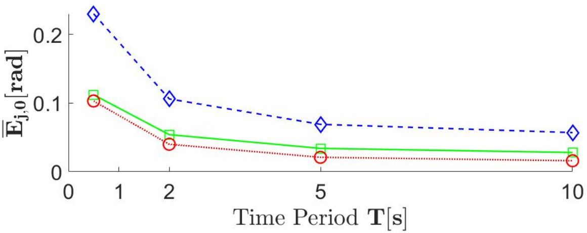
| Time Period, [s] | [rad] | [rad] | [rad] |
|---|---|---|---|
| 0.5 | 0.112 | 0.230 | 0.103 |
| 2 | 0.054 | 0.106 | 0.040 |
| 5 | 0.034 | 0.069 | 0.021 |
| 10 | 0.028 | 0.057 | 0.016 |
4.2 ILC methods
The MIMO ILC experiments followed Algorithm 1 to correct positioning errors during fast cleaning, with time period s.
4.2.1 Initial input
In the initial ILC step , the desired output was selected as the desired joint angles computed from the known desired brush-tip trajectory using Eqs. (49) to (51), as shown in Fig. 5. The initial input was applied to the SEA robot and the output was measured.

4.2.2 Perturbed input and model estimation
The input perturbation in ILC step can be selected to be frequency rich and provide the persistence of excitation needed for model acquisition [20]. represents the output caused by the input perturbation . For the experiments, the input perturbation was chosen to be the sum of chirp signals () and staircase functions (), with different patterns for each joint , as illustrated in Figure 7. The chirp functions were, for time and frequency hz,
and zero otherwise, where , with s for joint . For joint 2,
and zero otherwise, and for joint 3,
where , and the staircase functions consist of three consecutive 5-second steps starting from with magnitude equaling to and , and are zero otherwise. The parameters for each staircase function are tabulated in Table 2.
| staircase index | [s] | [rad] | [rad] | [rad] |
|---|---|---|---|---|
| 24 | +0.002 | -0.002 | +0.002 | |
| 23 | -0.003 | +0.003 | -0.003 | |
| 21 | +0.002 | -0.002 | +0.002 |
From linearity, the perturbation input-output relation was, from Eq. (1), .
With the system replaced by the Gaussian process as in Eq. (10), the observed perturbation for each joint angle , i.e., along with the input were used to estimate the model subsystems (with ) and the associated variance , from Eq. (14) and Eq. (15), through the input-weighted complex kernel as in Lemma 2. The necessary Fourier transforms and inverse Fourier transforms were computed in MATLAB. The SISO kernel was selected as where and denote the output variance and length scale, respectively. Then, the estimated subsystems and their variance are shown in Figure6.


4.2.3 Iteration gain selection
The iteration gain was selected to ensure ILC convergence based on the estimated model and uncertainty. Bounds on the model uncertainty were obtained from Eq. (25) of Lemma 4, with in Eq. (24) of Remark. 6. The iteration gains () were chosen to be for . Moreover, since the the desired output did not have significant frequency content beyond Hz, the iteration gains were reduced to zero after Hz, as for . The upper bound and the selected iteration gain are shown in Fig. 8.
4.2.4 Iterative input update
At each iteration step , the error during the active cleaning period () was computed using Fourier transform in MATLAB, and used to update the input to find the new input . For iteration step , the new input was updated based on input and error . Prior to the Fourier transform, the initial and final settling of the closed-loop controllers beyond the cleaning cycle were removed in all iterations by padding the error signal in time with zeros before and after the end of the cleaning cycles for s and thereby, the input was updated over the time interval .
4.3 Results & Discussion
The ILC led to improvement in the positioning precision of the brush with the SEA robot, even in the presence of significant contact effects. The reduction of the joint tracking error , with iteration step is shown in Figure 9 and the tracking results are shown in Figure 3.

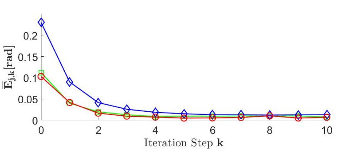
The joint tracking error decreased from initial values of rad, rad, rad at iteration step to final values of rad, rad, rad at iteration step . The final tracking errors were close to the repeatability of the system - the non-repeatable errors in the joint positioning of the robot were experimentally estimated to be rad at joints 1 and 3, and rad at joint 2. Thus, the ILC approach led to substantial reduction of 92% in joint , 94% in joint and 93% in joint in the tracking error.
An alternate approach to reduce the tracking error, without ILC, is to slow down the cleaning motion. In particular, with a time period s, the tracking error without ILC was rad, rad, rad. This is still larger than the final tracking error with ILC with a time period s, as seen by comparing the desired and actual output joint angles for the time period s without ILC in Fig. 3. Thus, the ILC enables at least 10-times increase in the operating speed for similar positioning precision with the SEA robot.
5 Conclusion
This work shows that the proposed complex-kernel Gaussian process regression with a proposed input-weighted kernel can sufficiently capture the model of a robot with series elastic actuators for precision operations even in the presence of contact effects, which in general are challenging to model a priori. Experimental results showed more than an order increase in operating speed and around 90% improvement in the positioning precision. Additionally, the work developed theoretical conditions to ensure convergence of an iterative learning controller for multi-input multi-output systems. However, the proposed approach is only valid locally around an operating point where the error caused by nonlinearity is sufficiently small (e.g., for local cleaning operations as demonstrated in the paper), and is not suitable for large-range motions with substantial nonlinearity. Our ongoing efforts are aimed at developing data-enabled methods to model and correct for such robot-pose-dependent nonlinearities.
References
- [1] Gill A. Pratt and Matthew M. Williamson. Series Elastic Actuators. IEEE/RSJ International Conference on Intelligent Robots and Systems, pages 399–406, 1995.
- [2] Nicholas Paine, Sehoon Oh, and Luis Sentis. Design and control considerations for high-performance series elastic actuators. IEEE/ASME Transactions on Mechatronics, 19(3):1080–1091, 2014.
- [3] L. Qui and E. J. Davison. Performance limitations of non-minimum phase systems in the servomechanism problem. Automatica, 29, March:337–349, 1993.
- [4] M. W. Spong. Modeling and control of elastic joint robots. ASME. J. Dyn. Sys., Meas., Control., 109(4):310–318., Dec 1987.
- [5] Steven Daniel Eppinger. Modeling robot dynamic performance for endpoint force control. Phd thesis, Massachusetts Institute of Technology, 1988.
- [6] Berk Altın and Kira Barton. Exponential stability of nonlinear differential repetitive processes with applications to iterative learning control. Automatica, 81:369–376, 2017.
- [7] Xiang Li, Yun-Hui Liu, and Haoyong Yu. Iterative learning impedance control for rehabilitation robots driven by series elastic actuators. Automatica, 90:1–7, 2018.
- [8] Jeremy G Stoddard, Georgios Birpoutsoukis, Johan Schoukens, and James S Welsh. Gaussian process regression for the estimation of generalized frequency response functions. Automatica, 106:161–167, 2019.
- [9] S. Arimoto, S. Kawamura, and F. Miyazaki. Bettering operation of robots by learning. J. of Robotic Systems, 1(2):123–140, March 1984.
- [10] S. Mishra and M.Tomizuka. Segmented iterative learning control for precision positioning of waferstages. In 2007 IEEE/ASME international conference on advanced intelligent mechatronics AIM, pages 1–6, Sept 2007.
- [11] A. de Luca and P. Lucibello. A general algorithm for dynamic feedback linearization of robots with elastic joints. In Proceedings. 1998 IEEE International Conference on Robotics and Automation (Cat. No.98CH36146), volume 1, pages 504–510 vol.1, May 1998.
- [12] B. Paden, D. Chen, R. Ledesma, and E. Bayo. Exponentially stable tracking control for multi-joint flexible manipulators. ASME Journal of Dynamic Systems, Measurement and Control, 115(1):53–59, 1993.
- [13] J. Ghosh and B. Paden. Nonlinear repetitive control. IEEE Transactions on Automatic Control, 45(5):949–954, 2000.
- [14] Yongqiang Ye and Danwei Wang. Clean system inversion learning control law. Automatica, 41(9):1549–1556, 2005.
- [15] Szuchi Tien, Qingze Zou, and Santosh Devasia. Iterative control of dynamics-coupling-caused errors in piezoscanners during high-speed afm operation. IEEE Transactions on Control Systems Technology, 13(6):921–931, 2005.
- [16] H.-S. Ahn, Y. Q. Chen, and K. L. Moore. Iterative learning control: Brief survey and categorization. IEEE Transactions on Systems, Man, and Cybernetics, Part C: Applications and Reviews, 37(6):1099–1121, 2007.
- [17] Kyong-Soo Kim and Qingze Zou. A modeling-free inversion-based iterative feedforward control for precision output tracking of linear time-invariant systems. IEEE/ASME Transactions on Mechatronics, 18(6):1767–1777, 2012.
- [18] Andreas Deutschmann, Pavel Malevich, Andrius Baltuška, and Andreas Kugi. Modeling and iterative pulse-shape control of optical chirped pulse amplifiers. Automatica, 98:150–158, 2018.
- [19] Robin de Rozario and Tom Oomen. Data-driven iterative inversion-based control: Achieving robustness through nonlinear learning. Automatica, 107:342–352, 2019.
- [20] Santosh Devasia. Iterative machine learning for output tracking. IEEE Transactions on Control Systems Technology, 27(2):516–526, 2017.
- [21] Yan Yan, Haiming Wang, and Qingze Zou. A decoupled inversion-based iterative control approach to multi-axis precision positioning: 3d nanopositioning example. Automatica, 48(1):167–176, 2012.
- [22] Nathan Banka, W Tony Piaskowy, Joseph Garbini, and Santosh Devasia. Iterative machine learning for precision trajectory tracking with series elastic actuators. In 2018 IEEE 15th International Workshop on Advanced Motion Control (AMC), pages 234–239. IEEE, 2018.
- [23] Nathan Banka, and Santosh Devasia. Application of iterative machine learning for output tracking with magnetic soft actuators. In IEEE/ASME Transactions on Mechatronics, (23)5:2186–2195, 2018.
- [24] Robin De Rozario, Juliana Langen, and Tom Oomen. Multivariable learning using frequency response data: a robust iterative inversion-based control approach with application. In American Control Conference (ACC), pages 2215–2220. IEEE, 2019.
- [25] C. E. Rasmussen and C. K. I. Williams. Gaussian Processes for Machine Learning. The MIT Press, Cambridge, MA, 2006.
- [26] Rafael Boloix Tortosa, Juan José Murillo Fuentes, Francisco Javier Payán Somet, and Fernando Pérez-Cruz. Complex gaussian processes for regression. IEEE transactions on neural networks and learning systems, 29(11):5499–5511, 2018.
- [27] Lennart Blanken and Tom Oomen. Kernel-based identification of non-causal systems with application to inverse model control. Automatica, 114:108830, 2020.
- [28] John Lataire and Tianshi Chen. Transfer function and transient estimation by gaussian process regression in the frequency domain. Automatica, 72:217–229, 2016.
- [29] Gianluigi Pillonetto, Francesco Dinuzzo, Tianshi Chen, Giuseppe De Nicolao, and Lennart Ljung. Kernel methods in system identification, machine learning and function estimation: A survey. Automatica, 50(3):657–682, 2014.
- [30] S. Devasia. Should model-based inverse inputs be used as feedforward under plant uncertainty? IEEE Trans. on Automatic Control, 47(11):1865–1871, Nov, 2002.
- [31] Esmaeil Naderi and Khashayar Khorasani. Inversion-based output tracking and unknown input reconstruction of square discrete-time linear systems. Automatica, 95:44–53, 2018.
- [32] Roger A Horn and Charles R Johnson. Matrix analysis. Cambridge university press, 2012.
- [33] Peter J Schreier and Louis L Scharf. Statistical signal processing of complex-valued data: the theory of improper and noncircular signals. Cambridge university press, 2010.