A low discrepancy sequence on graphs
Abstract
Many applications such as election forecasting, environmental monitoring, health policy, and graph based machine learning require taking expectation of functions defined on the vertices of a graph. We describe a construction of a sampling scheme analogous to the so called Leja points in complex potential theory that can be proved to give low discrepancy estimates for the approximation of the expected value by the impirical expected value based on these points. In contrast to classical potential theory where the kernel is fixed and the equilibrium distribution depends upon the kernel, we fix a probability distribution and construct a kernel (which represents the graph structure) for which the equilibrium distribution is the given probability distribution. Our estimates do not depend upon the size of the graph.
Keywords: Equal weight quadrature on graphs, potential theory on graphs, density approximation on graphs, Leja points on graphs.
1 Introduction
In many applications, the data is not represented by points in a high dimensional Euclidean space, but instead as vertices of networks with pairwise relations. A common problem that arises is estimating the mean or some integral of a function on those vertices, under the assumption that the function is smooth in an appropriate sense with respect to the network. For example, prior to elections, polls are used to estimate the opinions of a networked population about the candidates in expectation [17]. In environmental monitoring, estimating average temperature or water quality from a network of sensors allows governments to take preventative action [22]. In health policy, monitoring the average level of health and happiness in various populations requires extensive random polling [40, 10], which could be vastly downsampled with knowledge of the social networks of the population. Finally, in semi-supervised and active learning using Graph Neural Networks, the generalization error is specified as the average of the loss function associated with all vertices in a graph [20, 49].
In real world networks, evaluating the function at every vertex, or even at a large number of vertices, is very impractical. Therefore, an important question is how to choose a smaller subset of the vertices at which to evaluate the function and estimate the desired integral. Approaches such as Monte-Carlo integration are independent of the network, and do not exploit the assumption that the function is smooth with respect to the network. Methods that exploit the geometry of the domain, including potential theory estimates [14, 4, 1] and quasi-Monte-Carlo sampling [12], are only defined for intervals and compact vector spaces, and only for particular measures.
The purpose of this paper is to investigate deterministic constructions of low discrepancy sequences on undirected graphs, where the integration is taken with respect to an arbitrary measure, supported on the entire vertex set of the graph. We will use potential theory ideas, in particular, study a construction analogous to the so called Leja points. In contrast to classical potential theory, we start with a given measure and a graph, and modify the weights on the graph so that the given measure is the equilibrium measure.
1.1 Related work
Let be any measure space, be a probability measure on , be a random variable on with for almost all , . Then if , is sufficiently large, and are random samples from , then it is well known (for example, using Bernstein concentration inequality) that with -probability ,
| (1.1) |
Of course, deterministic variants of this inequality can be obtained using different kinds of deterministic assumptions on . For example, an equivalent formulation of a theorem of Erdős and Turán [14] is the following. Let be a sequence of monic polynomials, and . Then for any function having a bounded total variation on , we have
| (1.2) |
Theorems of this kind are known as discrepancy theorems. Although this estimate cannot be improved in general, it was improved by Blatt [4] with additional assumptions as follows. Let the points , and . Then there exists a contant such that
| (1.3) |
Both of these estimates depend heavily on potential theory estimates; in particular, the fact that is the logarithmic capacity of , and the measure of integration above is the equilibrium distribution for . There a is large amount of research devoted to generalization of this work including those involving potential theory in higher dimensions. In particular, an analogue of (1.3) in the case of arbitrary measures rather than equilibrium measures is given in [5]. A survey can be found in the book [1] of Andrievskii and Blatt.
The problem is of interest also in the theory of information based complexity where one seeks to approximate an integral over high dimensional spaces with averages of samples of the integrand. These have a different flavor, where instead of thinking in terms of zeros of polynomials and potential theory arguments, the interest is in devising quasi-Monte-Carlo systems with low discrepancy; i.e., system of points for which an estimate analogous to (1.3) holds, especially where the dependence of the constants on dimension are desired to have a polynomial growth with respect to the dimension. Most of these estimates are in the context of integration of -periodic functions on with respect to the Lebesgue measure and the total variation is taken in the sense of the so called Hardy-Kraus variation. A survey can be found in the book [12] of Dick and Pillichshammer. Methods have also been proposed to create a low discrepancy sequence through an accept/reject model for uniform random variables [13]. Existence theorems in the context of general measures and domains are also known in the literature, based mostly on probability theory ideas [31, 32]. We note finally that the emphasis here is on approximation of an integral by an unweighted average of the samples of the integrand, not on quadrature formulas where a suitably weighted average of the samples can yield substantially better estimates under various smoothness assumptions on the integrand.
The question of function approximation based on samples of the target function on a graph are well studied, especially in the context of band-limited functions. For example, the papers [2, 8] discuss algorithms for obtaining points on a graph with the property that it is possible to reconstruct band-limited functions on the graph exactly using samples at these points. The question is studied from the point of view of compressive sensing in [38]. The paper [36] presents a detailed study of the space of band-limited functions on a graph and the sets of uniqueness for such functions. A key fact that characterizes such sets is that a Marcinkiewicz-Zygmund inequality holds for the space of band-limited functions involved. In turn, this leads to quadrature formulas exact to for integration of these spaces. In this paper, we deal with signals that are not necessarily band-limited; indeed, the notion of spectral decomposition of the graph Laplacian plays no role in our theory. On the other hand, our interest is in approximating integrals of functions rather than the functions themselves.
A standard reference on potential theory is the book [25] by Landkof. We are not aware of any prior work specifically for potential theory on graphs. However, there are a number of papers dealing with potential theory on locally compact spaces, e.g., [16, 34, 30]. The notion of a sequence of Leja points was introduced in [26] in the context of approximation of the equilibrium measure of a compact subset of the complex plane. A detailed analysis of the rate of convergence of the sequence of measures that associates the mass with the first points in this sequence to the equilibrium measure is given most recently by Pritsker [37]. This notion of discrepancy theorems can be generalized in other, more general contexts. A survey can be found in [11] by De Marche, where computational issues are discussed. Discrepancy theorems for Leja points in the context of hyper-spheres is analyzed by Götz in [18].
After the submission of our paper, we came across a paper by Brown [6], where the author has given a construction of a sequence of good discrepancy points on a graph based on the Green function of a power of the graph Laplacian, where the discrepancy is measured in terms of the Wasserstein metric. Naturally, the error in integration is estimated analogously to the Hlawka-Koksma inequality [23] in terms of the Lipschitz constant of the function. In the current paper, we propose a construction independently of the eigen-decomposition of the graph Laplacian, and estimate the discrepancy using the matrix involved in our construction.
There has been recent interest in coreset selection on general domains, including graphs. A general selection of points that are well distributed on graphs has been found through randomized QR decompositions [3], and through random walk sampling [19, 33], however these results do not provide estimates on the error in approximation of an integral. There has also been significant work on sample selection for full reconstruction of the underlying signal (see [45] for a review of methods). In [44], the author provided bounds to guarantee the existence of quadrature formulas (known in the paper as graphical designs), which find exactly the averages of eigenfunctions of the graph Laplacian corresponding to large eigenvalues. In [27], the authors provide bounds for the quadrature error in computing the average of function values based on the values of the function at arbitrary points and quadrature weights. These bounds apply only for spectrally band limited functions. The bounds depend upon the spectral band, the norm of the target function, and certain powers of the graph Laplacian applied to the vector of the quadrature weights involved. Algorithms to choose these points and weights can be found in [28] for manifolds and [46] for a greedy algorithm of point and weight selection on graphs.
1.2 Motivating Example
As an example, in Figure 1 we display a quasi-Monte-Carlo sampling scheme on the unit square and compare it to the various proposed sampling schemes from this paper. For the quasi-Monte-Carlo sampling, we use a Halton sequence on the unit square, skipping the first 1000 samples and with a leap of 100 [47]. For our proposed methods, we begin with 10,000 points uniformly sampled on the unit square , and build a 50-nearest-neighbor graph. The weighted edges are computed using: a Gaussian weight , or a log potential weight with . We select 1000 Leja points using the algorithm and construction proposed in Sections 2.3 and 4.1. For each graph adjacency type, this is done for two different measures that we wish to integrate against: a uniform distribution on , or a nonuniform radial measure where .
It is clear from this example that the proposed graph Leja points with a uniform distribution recover a similar low discrepancy layout to quasi-Monte-Carlo sampled points. And beyond this, the graph Leja points are able to generalize to a non-uniform distribution with the same framework. But the true benefit of this proposed Leja point construction is that the algorithm applies in the case of an arbitrary graph, and will still result in well-spaced points.
 |
 |
 |
| Original graph | Leja Points, Gaussian, Unif. measure | Leja Points, Gaussian, radial measure |
 |
 |
 |
| Halton QMC sequence | Leja Points, Potential, Unif. measure | Leja Points, Potential, radial measure |
1.3 Outline of the paper
We describe our main theorem in Section 2 after reviewing some basic facts from potential theory in the abstract. As mentioned earlier, our approach is not to start with a matrix and work with whatever equilibrium measure is associated with it, but rather to start with a graph adjacency matrix and a given probability distribution on the vertices of the graph, and construct another matrix with the same properties as the graph for which this distribution is the equilibrium distribution. We describe three such constructions in Section 3. The theory is illustrated with various synthetic and real world examples in Section 4. The proof of the results in Section 2 are given in Section 5.
2 Main theorem
We develop some basic notation in Section 2.1, and review a fundamental theorem in potential theory in Section 2.2. The notion of Leja points is defined in Section 2.3. Our main theorem, Theorem 2.1 shows that the sequence of Leja points is a low discrepancy sequence for integration with respect to the given measure .
2.1 Notation
Let be a symmetric matrix, be a finite set with . We prefer to index with .
We consider any function to be a measure on as well as a function on , as well as a vector. So, for any function ,
| (2.1) |
For measures on , we use the notation
| (2.2) |
In particular, is the -th component of . The class of all probability measures on is denoted by . The class of all measures for which for all is denoted by .
We denote the vector by .
A matrix is conditionally positive semi-definite (c.p.s.d.) if for all with , and conditionally positive adefinite (c.p.d.) if it is c.p.s.d. and , together imply that .
For a symmetric matrix , we denote
| (2.3) |
For a vector , we denote the norm of by , and write .
2.2 Potential theory
A measure is the equilibrium measure (vector) if
| (2.4) |
In the context of complex potential theory, the quantity is often called Robin’s constant. In our context, we refer to the quantity as the capacity of .
An important characterization of the equilibrium measure is given by the following lemma, known generically as Frostman theorem. A proof can be found in almost any book on classical potential theory (e.g., [25, pp. 136-137] in the context of potentials on Euclidean spaces and [34, Theorem 2.1] in the context of locally compact spaces). We will reproduce a proof for the sake of completion in Section 5.
Lemma 2.1
(a) If is any equilibrium measure, and is the support of , then
| (2.5) |
and
| (2.6) |
(b) Let be conditionally positive semi-definite. If , and any measure with support satisfies both
| (2.7) |
and
| (2.8) |
then , and is an equilibrium measure. If is any equilibrium measure, then .
2.3 Leja points
In this section, we will assume a symmetric, conditionally positive semi-definite matrix , which has as an equilibrium measure. In particular,
| (2.9) |
Definition 2.1
A sequence of points in will be called a Leja sequence (with respect to a matrix ) if for every ,
| (2.10) |
The points will be referred to as Leja points.
Remark 2.1
The points are in general not distinct. In fact, in order for Theorem 2.1 to hold, the points will need to be repeated to be commensurate with the measure . Second, a Leja sequence is not uniquely determined by the initial point , since the definition does not require the to be unique.
We will denote the Dirac delta at by . For , let . Then
| (2.11) |
If is the range of , we write
| (2.12) |
Example 2.1
Let be any positive definite, matrix, be the class of all convex combinations of columns of . If , then .
Example 2.2
Let be the weighted adjacency matrix of a connected graph that does not have non-trivial, bipartite connected subgraph, and be the graph Laplacian, and be the set of eigenvalues of , and be the corresponding orthonormalized eigenvectors. Then ([9, Lemma 1.7]) . We let . Then is positive definite with non-negative entries, and positive diagonal, so that Theorem 2.1 is applicable, and the equilibrium measure for is defined uniquely. In particular, is invertible. If , , then
Let and be the class of all -band-limited functions; i.e., the class of all for which if . For , a crude estimate for is given by
Our main theorem is the following.
Theorem 2.1
Let for all , be a Leja sequence with respect to , be an equilibrium measure for , and be in the range of . Then
| (2.13) |
Remark 2.2
Remark 2.3
We note that the rate of convergence of the equal weight quadrature formulas is much faster than what is expected for quasi-Monte Carlo methods, demonstrating that the sequence of Leja points is a low discrepancy sequence in the sense of [12]. It is not clear what conditions on the matrix will ensure an equilibrium measure in . In Section 3, we will give a variety of possible constructions to modify either an arbitrary matrix or a matrix with certain properties to ensure that any given vector is an equilibrium measure of the resulting matrix. Thus, rather than taking the viewpoint that is given and is its equilibrium measure, we will start with and construct with as the equilibrium measure. Then the Leja sequence depends upon via .
The proof of Theorem 2.1 mimics the standard proof of the convergence of the measures in classical potential theory. Thus, we note that the mapping is a semi-inner product on the space of all measures on . We prove first that the sequence converges to in the sense of the semi-norm defined by this semi-inner product. This implies in turn that the Cesáro means of the sequence converges to . A tauberian argument then completes the proof. Of course, we need to keep track of the rates of convergence at each stage.
3 Constructions
Let be any symmetric matrix, and . We want to construct a matrix such that is conditionally positive semi-definite, and , so that is the equilibrium vector for . We describe three constructions.
3.1 Diagonal modification
This construction gives a modified graph Laplacian, and works with any symmetric matrix with no further assumptions. First, we construct a symmetric matrix so that .
We define the -Laplacian by
| (3.1) |
Then with ,
| (3.2) |
Let , and
| (3.3) |
Then
So, is diagonal dominant, hence, positive definite, and
| (3.4) |
so that is the unique equilibrium measure of and
| (3.5) |
Moreover,
| (3.6) |
Remark 3.1
The construction of the -Laplacian works for all symmetric matrices with no further assumptions. In the case when is the (weighted) adjacency matrix with non-negative weights, then with , is another adjacency matrix for the same graph so that if and only if . The matrix is the non-normalized graph Laplacian for . Thus, the eigenvalues of are the same as those of , and if is an eigenvector of , then the eigenvector for for the same eigenvalue is . In particular, is positive semi-definite, and the graph is connected if and only if is the unique null vector for .
3.2 Householder transform
In the case when is not invertible, there is another way to construct , which essentially preserves the eigenstructure of itself (rather than a graph Laplacian for ). This construction is also applicable for every non-invertible which may have negative entries. If and are unit vectors, the Householder transform is defined by
| (3.7) |
Clearly, is a symmetric unitary matrix, , and , so that . We have
| (3.8) |
Since is not invertible, there is a unit vector such that . Writing for the unit vector along , we set
| (3.9) |
Clearly, ,
| (3.10) |
The matrix has the same eigenvalues as , and if is the spectral decomposition of , then the eigenvectors of are obtained simply by replacing every eigenvector of by . However, this construction depends upon having a null vector and our ability of compute , and the norms will depend upon the norms of this Householder transform.
3.3 Symmetric scaling
This construction applies only to symmetric, non-negative matrices , and results in a matrix with the same eigenvalues as those of . For a matrix , and subsets , we denote by the sub-matrix of obtained by extracting rows of indexed by and columns of indexed by .
Let be a non-negative, symmetric matrix, satisfy the Brualdi condition
For all partitions of such that , we have
| (3.11) |
with equality holding if and only if .
Then a theorem of Brualdi [7] states that there exists a diagonal matrix with positive entries such that
| (3.12) |
Let be the diagonal matrix . Then satisfies
| (3.13) |
Clearly, represents a graph with the same vertices and edges as , except for different edge weights. We note that when has a positive diagonal, then the Brualdi condition is satisfied vacuously for every . The full algorithmic steps for finding such a bistochastic normalization of symmetric matrices can be found in [29, 24].
4 Experiments
4.1 Set up
One matrix that is trivially row-scalable as in (3.12) is the matrix of all positive entries; i.e., the graph is complete with self-loops at each vertex. Considering a complete matrix prevents a possible blow-up of on singleton vertices, where otherwise a singleton vertex would have . On the other hand, it is more expensive to apply the Sinkhorn algorithm [42] to a dense matrix than applying the algorithm to a sparse matrix , since the most expensive part of the algorithm is the matrix vector multiplications.
A sparse matrix can be augmented to have all positive entries in a style similar to Pagerank [35] by adding a small weighted edge between any pair of vertices,
| (4.1) |
Then trivially satisfies the assumptions in Section 3.3 since it has a positive diagonal. Moreover, because of the particular structure of , it is possible to compute a matrix vector multiplication in a time that depends only on the sparsity of . This is done using the trivial observation that
| (4.2) |
This observation of the Pagerank modification was originally made in [21].
Similarly, the matrix used in (2.10) can be constructed from the sparse matrix by observing that
| (4.3) |
where .
The entire algorithm for constructing the Leja points of the Pagerank graph in Eq. (4.1) is shown in Algorithm 1 for completeness. The computational complexity of the algorithm is mostly rooted in the Sinkhorn iterations for computing . Let be an matrix with edges per node (the number of edges need not be fixed, but simplifies the complexity calculation). Then each matvec operation requires flops, so computation of also requires flops. Exact bounds on the number of Sinkhorn iterationsis not known, but we can still denote the computational complexity as . Computing similarly requires flops and can be held in memory using sparse storage using (4.3). Finally, computing the Leja points requires summing up to columns of , which has computational complexity . This gives a total complexity of .
Input: Sparse matrix , Pagerank factor , Base measure , Number Leja points , Queryable function
Output: Integral estimate
In all the experiments below, we compare three quantities:
- •
the average , where is sampled randomly (with replacement) according to a weighted probability . This is denoted “Random” and with blue curves in the experiments.
- •
the average , where are the Leja points of the graph with equilibrium measure . This is denoted “Leja” and with red curves in the experiments.
- •
the average (cf. (5.7)), where the are the Leja points of the graph with equilibrium measure . This quantity is considered as a natural weighting of the Leja points that respects the order in which they are drawn. This is denoted “Summability” and with orange curves in the experiments.
We also note for all examples to follow in this section, that because both the Leja point selection algorithm and the Monte Carlo sampling are with replacement, it is possible to compute iterations without selecting all vertices. This additional sampling can be seen as establishing weights, as a point sampled twice is given twice the weight as a point sampled once. Additionally, we will use the Pagerank kernel as in (4.1) with .
Finally, unless otherwise noted,we set to be the inverse of the kernel density estimate for the graph,
| (4.4) |
normalized so that . This is an arbitrary choice of , as the only required condition is for , and is meant to demonstrate that the results apply to more than . This equilibrium measure is of particular interest because, in the point cloud kNN graph setting, it approximately cancels out the sampling density of the points themselves. More specifically, if the points are sampled from the density that has comptact supp, then
| (4.5) |
which would be independent of the relative heights of the sampling density. However, any positive density satisfies the necessary assumptions for the proven approximation rates.
4.2 Synthetic Graphs with Smooth Functions
A common model for social networks is a so-called small world network [48]. Small world networks are graphs with a small number of edges per vertex, but where any pair of vertices is likely to have a small graph distance. Mathematically, if the average graph distance between two vertices is , a small-world graph with vertices roughly satisfies . These networks are antithetical to nearest neighbor graphs that are generated from a point cloud in some metric space, and have a large network diameter.
 |
 |
| (a) | (b) |
 |
 |
| (c) | (d) |
In the first set of experiments, we examine the quadrature approximation for a smooth function on a Watts-Strogatz model [48]. This is a model of random graph generation that exhibits small-world properties, including low path distances between vertices while still exhibiting a high degree of clustering. The model takes inputs of number of vertices, average number of edges per vertex, and a parameter that models the fraction of random connections. When the generated graphs will exhibit lattice structure, and when the graph will resemble an Erdős-Rényi random graph.
In this experiment, we take to be the coordinate of the vertex locations after applying a force layout [15]. This results in a smooth function in the nodes, since a force layout is a heuristic algorithm that repels unconnected nodes away from one another. The functions are displayed in Figure 2, and the graphs are constructed for various values of the parameter , which measures the level of structure in the graph. Also, because the graph can be regenerated, we run the experiment for 1000 graphs with the same parameters. We display the mean and standard deviation across these 1000 instantiations of the graph. For each graph, we take vertices, and an average of 25 edges per node.
In a second set of experiments, we construct a nearest neighbor graph from the point cloud in Figure 3. The interesting aspect of this data set is that the points from the two clusters are sampled in a highly non-uniform manner. Because is constructed by approximating the inverse of the local density, this results in a similar number of points sampled from both clusters, see Figure 4. The function is taken to be the -coordinate of the points. Again, because the graph can be regenerated, we run the experiment for 1000 graphs with the same parameters. We display the mean and standard deviation across these 1000 instantiations of the graph. For each graph, we take nodes and use a bandwidth for the Gaussian kernel of .
 |
 |
We also demonstrate that the location of the Leja points for each of these data sets, using to be an inverse density estimate, in Figure 4.
 |
 |
 |
| WS graph | WS graph | Two Cluster metric graph |
4.3 Synthetic Graphs with Non-Band-Limited Functions
A novelty of the results in Theorem 2.1 is that it applies to fuctions that are not required to be band limited.
We demonsrate the strengths of the bound in Eq. (2.13), namely that the function is not required to be band limited in order for the estimation bounds to apply. To characterize this, we generate a series of experiments on the two cluster data from Figure 3, but with a significantly more complicated function . To construct , we consider a spectral decomposition of the matrix . Then we construct the function spectrally via
| (4.6) |
where , and controls the rate of spectral decay with respect to the eigenvalue . In Figure 5, we demonstrate the quadrature approximation error averaged across instantiations of the random graph and random function. We also consider these experiments across varying , demonstrating empirically the effect of the spectral decay rate on the overall quadrature approximation rate.
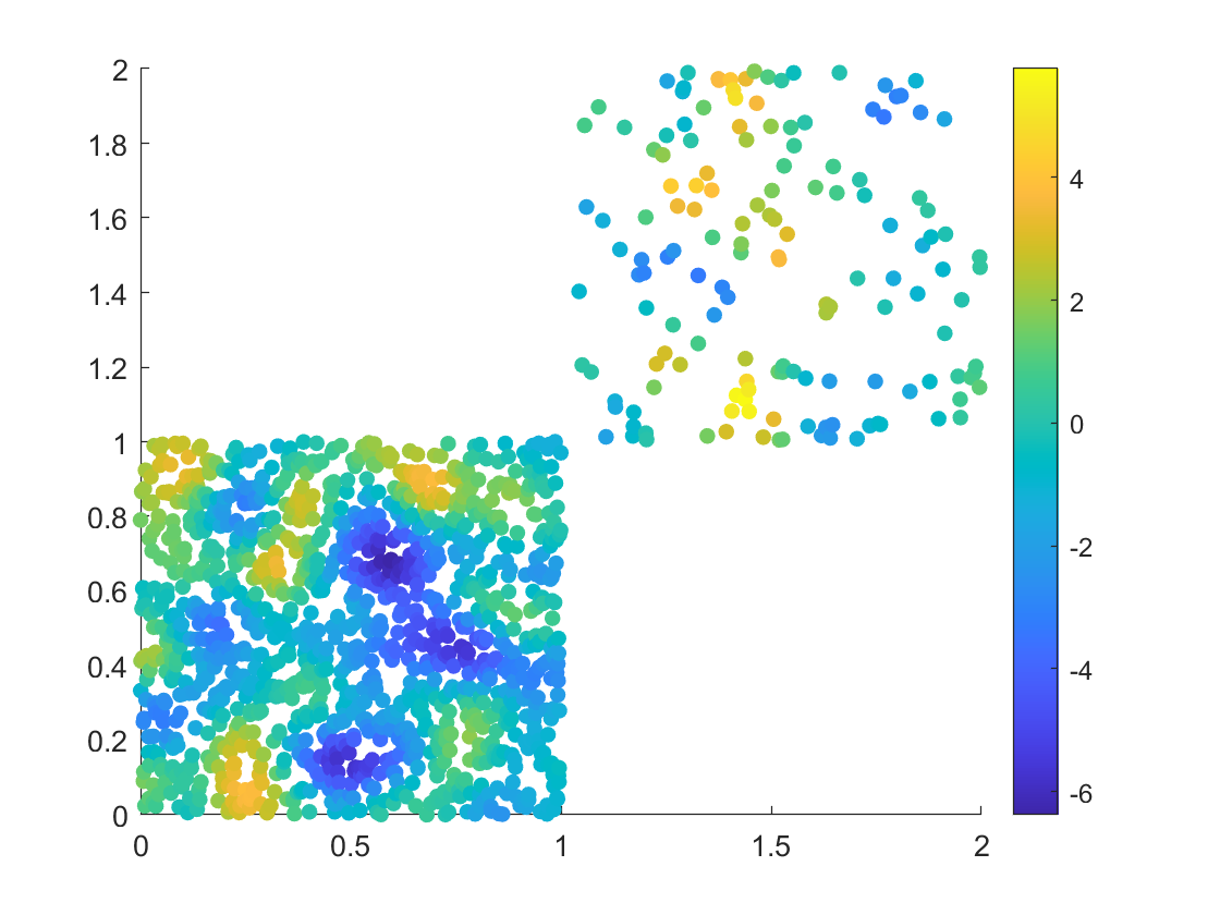 |
 |
| Data and Function Example | Fast spectral decay |
 |
 |
| Medium spectral decay | Slow spectral decay |
Figure 5 shows an reduction in the gap between the Monte Carlo quadrature approximation rate and the Leja point approximation rate as the spectral decay tail increases. This is to be expected, as a larger spectral tail reduces the smoothness of the function with respect to the graph. But this experiment does show that Leja point quadrature approximation rate does have a benefit over random sampling without the requirement that the target function be spectrally band-limited.
4.4 Real-World Graphs
Next, we illustrate our theory using a couple of real world graphs and functions. Since the graph is fixed in these examples and cannot be regenerated, we compute the Leja sequence for different random choices of , and average the errors. Similarly for the Monte Carlo comparison, we generate different sequences of sampled points.
In this first set of experiments, we examine the quadrature error for labels from the CORA data set [41]. The standard form of the data set comprises a digraph with 2708 publications as vertices, and edge from to means that paper cited paper . These publications are from seven areas of computer science and information theory, which corresponds to the 7 different classes in the data set. There are a large number of weakly connected components, many of which are singletons. The largest weakly connected component has nodes. We treat the citation links as undircted edges and construct a binary, symmetric adjacency matrix , and take the largest connected component as the graph. This is equivalent to the largest weakly connected component, which results in an undirected graph with vertices.
Due to the sparsity of the number of edges in this graph, using the matrix constructed directly from the graph results in a slow rate at which changes as the number of Leja points increases. The process is expedited if we extend the connections between documents to two steps away by taking . In this experiment in Figure 6, we take the function to be the indicator function of class for . These labels represent the field of the given document, and are related to the network due to the obvious fact that papers in the same field are more likely to cite one another.
 |
 |
 |
 |
| Data and Labels | Label 1 | Label 2 | Label 3 |
 |
 |
 |
 |
| Label 4 | Label 5 | Label 6 | Label 7 |
In the second set of experiments, we examine the exepcted value approximation for positive association with various propositions in the Proposition dataset [43, 50]. The November 2012 California ballot contained 11 initiatives, or propositions, on a variety of issues, including state taxation, corrections, and food labelling among others. The data consist of Twitter posts related to initiatives, grouped according to different propositions. For each proposition, the data is a directed graph with edge from to if the tweet originated from user to user . The authors of [43] have assigned an evaluation of the emotion of the sender with each tweet. We treat the edges as undirected and construct a binary, symmetric adjacency matrix . We take the largest connected component of the graph for these experiments. Each proposition has its own graph, with a positive or negative label of sentiment on each node. The mean binary sentiment estimate could be used as a proxy for the number of people that would vote for/against the proposition.
Due to the sparsity of the number of edges in this graph, we extend the connections between documents to two steps away by taking . In this experiment, we take the function to be a binary indicator function ( or ) of whether the sentiment is positive. We examine two different graphs in Figure 7, those for Proposition 30 and those for Proposition 37, as those are the graphs with the largest number of vertices, with vertices for Prop 30 and vertices for Prop 37.
As we can see in both the Cora experiments and the Proposition experiments, the Leja quadrature error performs better than the average Monte Carlo performance even for a small number of sampled points. We also wish to address the relative lack of smoothness of the quadrature approximations relative to the synthetic experiments and the Monte Carlo trials. First, recall that the labels here are incredibly non-smooth as they are binary. Second, we note that the Leja point sampling can be thought of as a distance sampling scheme, choosing consecutive points far apart from one another and points likely to have different labels. Because of these points, the approximation error will have a larger local variability than random sampling, even when averaged across multiple initializations. This is also a motivation for using the summability approximation, which applies a decaying weight to added points and does not demonstrate the same local fluctuations as the unweighted Leja point averages.
 |
 |
| (a) | (b) |
 |
 |
| (c) | (d) |
We also demonstrate that the location of the Leja points for each of these data sets, using to be an inverse density estimate, in Figure 8.
 |
 |
 |
| Prop 30 | Prop 37 | Cora |
4.5 Additional Comparisons
In this section, we compare our method to a natural alternative: computing a function interpolation from the sampled subset to the entire set of vertices , and then integrating that estimate against . A recent method for this function interpolation is graph sampling set selection (GSSS) [39], which is built on taking a weighted linear combination of columns of the spectrally filtered graph Laplacian. We compare to this method in Figure 9 on the community graph data set proposed in [39]. We compare using both the original adjacency matrix , and using the two-hop adjacency matrix , as the starting set of edges. We take to be the inverse density of each community, normalized. Again, we compare across 1000 instantiations of the graph with points, and report the mean and standard deviation of the error at each fraction of points kept. The function being regressed in each instantiation is chosen to be constant on each community, with the value randomly choosen from a uniform distribution.
 |
 |
| (a) | (b) |
 |
 |
| (c) | (d) |
Finally, we demonstrate that the bound (2.13) on the quadrature error is independent of the number of data points for problems of fixed complexity. In this experiment, we return to the two cluster example from Figure 3 while varying the number of data points. The graph created from this point cloud remains fixed, constructed with a Gaussian kernel of bandwidth . In Figure 10, we vary the number of data points and plot the quadrature error for a fixed number of Leja iterations. After an initial level-off as the number of points grows, the error is more or less constant. This shows that the error does not have a strong dependence on for neighbor graphs built from a fixed sampling distribution.
 |
 |
| 100 Leja Iterations | 1000 Leja Iterations |
5 Proofs
Proof of Lemma 2.1.
Let be an equilibrium measure. If , then for all , , and therefore, is a minimum for
So, . This implies (2.5). Let and, in this proof only, . Then
Therefore, . Since is a finite set, this implies (2.6).
Next, let be conditionally positive semi-definite, and satisfy the conditions of part (b). Then (2.8) shows that , and (2.7) shows that . So,
Thus, . Since is an equilibrium measure, it follows that , so that is also an equilibrium measure. Also, , so that is in the null space of .
The next theorem shows in a standard manner than the sequence associated with the Leja points converge to the equilibrium measure.
Theorem 5.1
We have
| (5.1) |
Any weak-star limit of a subsequence of is also an equilibrium measure.
Proof. We have for ,
| (5.2) | ||||
In view of the definition (2.11) of Leja points,
| (5.3) |
Integrating both sides with respect to and using (2.9), we get for all ,
Therefore, (5.2) leads to
| (5.4) |
In view of (2.9),
Therefore, (5.4) implies (5.1). In turn, if be any subsequence of converging weak-star to a probability measure , then (5.1) shows that . Therefore, is also an equilibrium measure.
We note a couple of corollaries of the proof of Theorem 5.1.
Corollary 5.1
For ,
| (5.5) |
We formulate the next corollary as a theorem in its own right.
Theorem 5.2
Let . Then for all , ,
| (5.6) |
In particular,
| (5.7) |
Proof. The first estimate in (5.6) follows from the first estimate in (5.5) and (5.3). The second estimate in (5.6) follows from the fact that
| (5.8) |
The final inequality in (5.6) following from the fact that . We observe now that
| (5.9) |
Therefore, (5.7) follows from (5.6) and the fact that for all .
Theorem 5.3
If for all , we have for ,
| (5.10) |
Proof. For , we have
i.e.,
Therefore, for any with , a summation in the above inequality leads to
Since , Corollary 5.1 now shows that
Rearranging,
For , this gives
For any , we have and . Therefore,
In the reverse direction, we recall (5.8). Together with (5.6), this leads to (5.10).
Proof of Theorem 2.1.
Acknowledgments
The work of AC was supported in part by NSF DMS grants 2012266, 1819222, and Sage Foundation Grant 2196. The work of HNM is supported in part NSF DMS grant 2012355 and ARO grant W911NF2110218. We thank Professors Percus at Claremont Graduate University for his help in securing the Proposition data set, which was sent to us by Dr. Linhong Zhu at USC Information Sciences Institute in Marina Del Ray, California.
References
- [1] V. V. Andrievskii and H.-P. Blatt. Discrepancy of signed measures and polynomial approximation. Springer Science & Business Media, 2013.
- [2] A. Anis, A. Gadde, and A. Ortega. Efficient sampling set selection for bandlimited graph signals using graph spectral proxies. IEEE Transactions on Signal Processing, 64(14):3775–3789, 2016.
- [3] A. Bermanis, A. Averbuch, and R. R. Coifman. Multiscale data sampling and function extension. Applied and Computational Harmonic Analysis, 34(1):15–29, 2013.
- [4] H.-P. Blatt. On the distribution of simple zeros of polynomials. Journal of approximation theory, 69(3):250–268, 1992.
- [5] H.-P. Blatt and H. N. Mhaskar. A general discrepancy theorem. Arkiv för Matematik, 31(2):219–246, 1993.
- [6] L. Brown. Sequences of well-distributed vertices on graphs and spectral bounds on optimal transport. Journal of Fourier Analysis and Applications, 27(2):1–27, 2021.
- [7] R. A. Brualdi. The DAD theorem for arbitrary row sums. Proceedings of the American Mathematical Society, 45(2):189–194, 1974.
- [8] S. Chen, R. Varma, A. Sandryhaila, and J. Kovačević. Discrete signal processing on graphs: Sampling theory. IEEE transactions on signal processing, 63(24):6510–6523, 2015.
- [9] F. R. K. Chung. Spectral graph theory, volume 92. American Mathematical Soc., 1997.
- [10] A. Cloninger, B. Roy, C. Riley, and H. M. Krumholz. People mover’s distance: Class level geometry using fast pairwise data adaptive transportation costs. Applied and Computational Harmonic Analysis, 47(1):248–257, 2019.
- [11] S. De Marchi. On Leja sequences: some results and applications. Applied mathematics and computation, 152(3):621–647, 2004.
- [12] J. Dick and F. Pillichshammer. Digital nets and sequences: discrepancy theory and quasi–Monte Carlo integration. Cambridge University Press, 2010.
- [13] R. Dwivedi, O. N. Feldheim, O. Gurel-Gurevich, and A. Ramdas. The power of online thinning in reducing discrepancy. Probability Theory and Related Fields, 174(1-2):103–131, 2019.
- [14] P. Erdős and P. Turán. On the uniformly-dense distribution of certain sequences of points. Ann. of Math, 41:162–173, 1940.
- [15] T. Fruchterman and E. Reingold. Graph drawing by force-directed placement. Software — Practice and Experience, 21(11):1129–1164, 1991.
- [16] B. Fuglede. On the theory of potentials in locally compact spaces. Acta mathematica, 103(3-4):139–215, 1960.
- [17] D. Gayo-Avello. A meta-analysis of state-of-the-art electoral prediction from twitter data. Social Science Computer Review, 31(6):649–679, 2013.
- [18] M. Götz. On the distribution of Leja-Górski points. Journal of Computational Analysis and Applications, 3(3):223–241, 2001.
- [19] L. Jin, Y. Chen, P. Hui, C. Ding, T. Wang, A. V. Vasilakos, B. Deng, and X. Li. Albatross sampling: robust and effective hybrid vertex sampling for social graphs. In Proceedings of the 3rd ACM international workshop on MobiArch, pages 11–16, 2011.
- [20] T. N. Kipf and M. Welling. Semi-supervised classification with graph convolutional networks. In Proceedings of ICLR, 2017.
- [21] P. A. Knight. The sinkhorn–knopp algorithm: convergence and applications. SIAM Journal on Matrix Analysis and Applications, 30(1):261–275, 2008.
- [22] A. Krause, J. Leskovec, C. Guestrin, J. VanBriesen, and C. Faloutsos. Efficient sensor placement optimization for securing large water distribution networks. Journal of Water Resources Planning and Management, 134(6):516–526, 2008.
- [23] L. Kuipers and H. Niederreiter. Uniform distribution of sequences. Courier Corporation, 2012.
- [24] B. Landa, R. R. Coifman, and Y. Kluger. Doubly stochastic normalization of the gaussian kernel is robust to heteroskedastic noise. SIAM Journal on Mathematics of Data Science, 3(1):388–413, 2021.
- [25] N. S. Landkof. Foundations of modern potential theory, volume 180. Springer, 1972.
- [26] F. Leja. Sur certaines suites liées aux ensembles plans et leur application à la représentation conforme. Annales Polonici Mathematici, 1(4):8–13, 1957.
- [27] G. Linderman and S. Steinerberger. Numerical integration on graphs: Where to sample and how to weigh. Mathematics of Computation, 89(324):1933–1952, 2020.
- [28] J. Lu, M. Sachs, and S. Steinerberger. Quadrature points via heat kernel repulsion. Constructive Approximation, 51(1):27–48, 2020.
- [29] N. F. Marshall and R. R. Coifman. Manifold learning with bi-stochastic kernels. IMA Journal of Applied Mathematics, 84(3):455–482, 2019.
- [30] H. N. Mhaskar. Weighted polynomials, radial basis functions and potentials on locally compact spaces. Numerical functional analysis and optimization, 11(9-10):987–1017, 1990.
- [31] H. N. Mhaskar. On the tractability of multivariate integration and approximation by neural networks. Journal of Complexity, 20(4):561–590, 2004.
- [32] H. N. Mhaskar. Dimension independent bounds for general shallow networks. Neural Networks, 123:142–152, 2020.
- [33] A. Nazi, Z. Zhou, S. Thirumuruganathan, N. Zhang, and G. Das. Walk, not wait: Faster sampling over online social networks. Proceedings of the VLDB Endowment, 8(6):678–689, 2015.
- [34] M. Ohtsuka et al. On potentials in locally compact spaces. Journal of Science of the Hiroshima University, Series AI (Mathematics), 25(2):135–352, 1961.
- [35] L. Page, S. Brin, R. Motwani, and T. Winograd. The pagerank citation ranking: Bringing order to the web. Technical report, Stanford InfoLab, 1999.
- [36] I. Pesenson. Sampling in paley-wiener spaces on combinatorial graphs. Transactions of the American Mathematical Society, 360(10):5603–5627, 2008.
- [37] I. E. Pritsker. Equidistribution of points via energy. Arkiv för Matematik, 49(1):149–173, 2011.
- [38] G. Puy, N. Tremblay, R. Gribonval, and P. Vandergheynst. Random sampling of bandlimited signals on graphs. Applied and Computational Harmonic Analysis, 44(2):446–475, 2018.
- [39] A. Sakiyama, Y. Tanaka, T. Tanaka, and A. Ortega. Eigendecomposition-free sampling set selection for graph signals. IEEE Transactions on Signal Processing, 67(10):2679–2692, 2019.
- [40] L. E. Sears, S. Agrawal, J. A. Sidney, P. H. Castle, E. Y. Rula, C. R. Coberley, D. Witters, J. E. Pope, and J. K. Harter. The well-being 5: development and validation of a diagnostic instrument to improve population well-being. Population health management, 17(6):357–365, 2014.
- [41] P. Sen, G. Namata, M. Bilgic, L. Getoor, B. Galligher, and T. Eliassi-Rad. Collective classification in network data. AI magazine, 29(3):93–93, 2008.
- [42] R. Sinkhorn and P. Knopp. Concerning nonnegative matrices and doubly stochastic matrices. Pacific Journal of Mathematics, 21(2):343–348, 1967.
- [43] L. M. Smith, L. Zhu, K. Lerman, and Z. Kozareva. The role of social media in the discussion of controversial topics. In 2013 International Conference on Social Computing, pages 236–243. IEEE, 2013.
- [44] S. Steinerberger. Generalized designs on graphs: Sampling, spectra, symmetries. Journal of Graph Theory, 93(2):253–267, 2020.
- [45] Y. Tanaka, Y. C. Eldar, A. Ortega, and G. Cheung. Sampling signals on graphs: From theory to applications. IEEE Signal Processing Magazine, 37(6):14–30, 2020.
- [46] S. Vahidian, B. Mirzasoleiman, and A. Cloninger. Coresets for estimating means and mean square error with limited greedy samples. In Conference on Uncertainty in Artificial Intelligence, pages 350–359. PMLR, 2020.
- [47] X. Wang and F. J. Hickernell. Randomized halton sequences. Mathematical and Computer Modelling, 32(7-8):887–899, 2000.
- [48] D. J. Watts and S. H. Strogatz. Collective dynamics of ‘small-world’networks. Nature, 393(6684):440–442, 1998.
- [49] Y. Wu, Y. Xu, A. Singh, Y. Yang, and A. Dubrawski. Active learning for graph neural networks via node feature propagation. arXiv preprint arXiv:1910.07567, 2019.
- [50] L. Zhu, A. Galstyan, J. Cheng, and K. Lerman. Tripartite graph clustering for dynamic sentiment analysis on social media. In Proceedings of the 2014 ACM SIGMOD international conference on Management of data, pages 1531–1542, 2014.