Modified virial theorem for highly magnetized white dwarfsModified virial theorem for highly magnetized white dwarfs–References
Abstract
Generally the virial theorem provides a relation between various components of energy integrated over a system. This helps us to understand the underlying equilibrium. Based on the virial theorem we can estimate, for example, the maximum allowed magnetic field in a star. Recent studies have proposed the existence of highly magnetized white dwarfs, with masses significantly higher than the Chandrasekhar limit. Surface magnetic fields of such white dwarfs could be more than G with the central magnitude several orders higher. These white dwarfs could be significantly smaller in size than their ordinary counterparts (with surface fields restricted to about G). In this paper we reformulate the virial theorem for non-rotating, highly magnetized white dwarfs (B-WDs) in which, unlike in previous formulations, the contribution of the magnetic pressure to the magnetohydrostatic balance cannot be neglected. Along with the new equation of magnetohydrostatic equilibrium, we approach the problem by invoking magnetic flux conservation and by varying the internal magnetic field with the matter density as a power law. Either of these choices are supported by previous independent work and neither violates any important physics. They are useful while there is no prior knowledge of field profile within a white dwarf. We then compute the modified gravitational, thermal and magnetic energies and examine how the magnetic pressure influences the properties of such white dwarfs. Based on our results we predict important properties of these B-WDs, which turn out to be independent of our chosen field profiles.
Keywords:
magnetic fields – white dwarfs – stars: general – stars: magnetic fields – stars: massive – MHD1 Introduction
White dwarfs are electron degenerate compact stars in which the outward degeneracy pressure force is able to balance the inward gravitational force only when the white dwarf mass is below the Chandrasekhar limit (Chandrasekhar 1935). In Newtonian calculations, the limiting mass of a carbon–oxygen white dwarf is , where is the mass of Sun, but this can be increased by rotation or magnetic fields (Ostriker & Hartwick 1968). White dwarfs are considered to be the progenitors of the type Ia supernovae which are some of the most widely studied astronomical events and explosions and rightfully so because of their usefulness to measure cosmic distances. Although not everything is understood about these events, the general consensus is that they are thermonuclear explosions of white dwarfs with masses very close to the Chandrasekhar limit. However recent observations of a fast-growing number of several peculiar, overluminous type Ia supernovae, for example SN 2006gz, SN 2007if, SN 2009dc and SN 2003fg, bring even this basic idea into serious question, because they are best explained by progenitor white dwarfs with super-Chandrasekhar masses in the range to (Howell et al. 2006; Scalzo et al. 2010).
One acceptable proposal is that these super-Chandrasekhar white dwarfs are highly magnetized white dwarfs (B-WDs) (Das & Mukhopadhyay 2013). This model was first formulated by Mukhopadhyay and his collaborators (Kundu & Mukhopadhyay 2012; Das & Mukhopadhyay 2012), who put the idea in the limelight. It has since been elaborated upon by various groups. Although the idea was further questioned by various authors, most, if not all, of the concerns that were raised against B-WDs have been addressed by Mukhopadhyay and his collaborators in subsequent publications. For instance, it was shown by Das & Mukhopadhyay 2014a; Das & Mukhopadhyay 2014b that the unreasonable possibility of a white dwarf (Dong et al. 2014; Coelho et al. 2014) is ruled out when magnetic energy density is appropriately included in magnetostatic balance and the mass equation simultaneously and self-consistently. Also, the maximum possible magnetic field sustainable in a B-WD and the energy content of various corresponding terms in the virial theorem (Coelho et al. 2014) were shown (Das & Mukhopadhyay 2014a) to be misleading, unless the virial theorem is established for a strong field. This was briefly explored by Mukhopadhyay & Rao 2016a and we elaborate upon it here in detail. Other authors (Chatterjee et al. 2017) argued, based on hypothetical pycnonuclear reaction rates, that super-Chandrasekhar O B-WDs are not possible but instead limited to less than . However, if their chosen pycnonuclear reaction rates are correct, even the Chandrasekhar limit for nonmagnetic, non-rotating white dwarfs has to be restricted to . This is counter-intuitive. However the pycnonuclear reaction rates are extremely uncertain and must be constrained carefully, more so than they have been. Moreover with the same pycnonuclear reaction rates C white dwarfs recover the Chandrasekhar limit and the underlying B-WDs are found to be super-Chandrasekhar. In fact later on, with more logical pycnonuclear reaction rates, Otoniel et al. 2019 showed that highly magnetized non-rotating super-Chandrasekhar white dwarfs are quite possible with masses grater than . So the issue of the pycnonuclear reaction is no longer problematic. On the other hand, it has been well-known since 1973 (Tayler 1973; Markey & Tayler 1973) that purely poloidal (or poloidally dominated) or purely toroidal fields are unstable. Hence any stability analysis of a magnetized star based on purely poloidal and purely toroidal field, as attempted by Bera & Bhattacharya 2016, does not make any sense (Mukhopadhyay et al. 2016). However, it was shown by Wickramasinghe et al. 2013 that a white dwarf with toroidally dominated mixed field configuration (with a small poloidal component) remains stable for a long time. In this case the white dwarf is approximately spherical in shape (Subramanian & Mukhopadhyay 2015). Hence, in a convenient stable mixed field configuration, we can always formulate a profile for the magnitude of magnetic field with respect to the stellar radius or density as we advocate here. Without prior knowledge of the variation of field magnitude within a star our simpler profiles chosen below are not at odds with any known physics or observations.
Nevertheless, there is another extensive set of independent work that supports the proposition of super-Chandrasekhar magnetized white dwarfs (Federbush et al. 2014; Franzon & Schramm 2015; Sotani & Tatsumi 2017; Franzon & Schramm 2017; Shah & Sebastian 2017; Moussa 2017; Roy et al. 2019, to list a significant selection). Recently, the Mukhopadhyay group explored the luminosity and possible gravitational radiation of rotating B-WDs. While Bhattacharya et al. 2018 and Gupta et al. 2020 showed that the B-WDs turn out to be too dim to detect, Kalita & Mukhopadhyay 2019 explored their gravitational waves, along with electromagnetic counterparts, of which the detectability by forthcoming instruments was further explored by Kalita & Mukhopadhyay 2019 and Kalita et al. 2020. Moreover, others often go beyond the idea of introducing strong magnetic fields and invoke additional physics, such as anisotropic pressure (Herrera & Barreto 2013), lepton number violation (Belyaev et al. 2015), modified gravity (Banerjee et al. 2017; Eslam Panah & Liu 2019), effects of net charge (Liu et al. 2014; Carvalho et al. 2018) and ungravity (Bertolami & Mariji 2016).
Here we explore the maximum possible magnetic fields and the mass needed to sustain a magnetized star, particularly a white dwarf, by modifying the virial theorem. Note that strong magnetic fields are expected to affect not only momentum balance (by magnetostatic balance for example) but also the underlying equation of state and thermal energy.
The virial theorem relates the integrated gravitational potential, kinetic, thermal and magnetic energies and provides an insight into the equilibrium of the system. Understanding the virial theorem for B-WDs helps us understand how high a magnetic field could be sustained therein and plausibly modify the properties of a normal white dwarf, thereby, making it a B-WD. In the weak field regime, the deviation of the Chandrasekhar limit owing to magnetic field has been explored earlier by Shapiro & Teukolsky 1983 and any changes to the properties of the white dwarf found to be only perturbative.
In the next section we recall the basic idea of scalar virial theorem, assuming the magnetic field is not perturbative. Subsequently, based on the magnetohydrostatic (rather than the hydrostatic) equilibrium, we compute various energy terms in virial equilibrium in section 3 for two model magnetic field profiles. In the beginning of the same section we also justify the chosen field profiles. In section 4 we discuss the results in detail and we end with conclusions in section 5.
2 The scalar virial theorem
The virial theorem is a general integral theorem which relates various components of energy. We use it to discuss the effects of high magnetic fields on white dwarfs, thereby making them B-WDs. The well known form of the virial theorem can be recalled as
| (1) |
for a dynamically stable star when the moment of inertia is constant (see Shapiro & Teukolsky 1983 or Eldridge & Tout 2019 for details). Here,
| (2) |
is a generalized moment of inertia and
| (3) |
| (4) |
| (5) |
and
| (6) |
are the kinetic, thermal, magnetic and gravitational energies respectively, when is the density, is the bulk velocity, is the pressure of stellar matter, is the magnetic field, is Newton’s gravitational constant, is the mass of the star of volume , is the radius from the centre of the star, is the elemental mass and is the corresponding volume.
Here we consider the case of a (static) non-rotating white dwarf for which . Hence, the scalar virial theorem reduces to
| (7) |
and this can be approximately recast to
| (8) |
(Shapiro & Teukolsky 1983; Mukhopadhyay & Rao 2016a), where , and are the constants, determined by the shape and other properties of the star investigated below, the magnetic flux through its surface , with being the average magnetic field and is the radius of the star. Here we consider the isotropic effects of an averaged magnetic field and so overall consider the star to be spherical in shape. For the plausibility of this, see numerical simulation results by Wickramasinghe et al. 2013 and Subramanian & Mukhopadhyay 2015, particularly for toroidally dominated cases.
Next we assume that a polytropic equation of state (EoS) is satisfied through the entire star such that , where and are the polytropic constants and , where is the mean density. The scalar virial theorem can then be reduced to
| (9) |
where . We have simply substituted from the EoS in equation (8) to arrive at the second term in equation (9).
Now rearranging equation (9), we obtain
| (10) |
for any . For , appropriate for extremely relativistic degenerate electrons, this becomes
| (11) |
which is independent of for a fixed magnetic flux, as expected from Chandrasekhar’s theory. This can be solved for . For , appropriate to high magnetic field and high density (Das & Mukhopadhyay 2013), equation (10) becomes
| (12) |
to give the mass explicitly.
3 Modification to the virial theorem
Here we evaluate the coefficients , and to establish the virial theorem at high magnetic field. First we note, very importantly, that in the presence of strong magnetic field, the upper limit for magnetic fields in white dwarfs, as discussed for weak field cases by Shapiro & Teukolsky 1983, must be revised because the contribution of the magnetic pressure to the magnetohydrostatic balance equation cannot be neglected. Here we attempt to revise it in a simpler framework. The new momentum balance condition, neglecting the effect of magnetic tension, is given by (Das & Mukhopadhyay 2014a, see for example)
| (13) |
at an arbitrary radius with mass enclosed at that radius , where includes the contribution from magnetic field and is the pressure owing to the magnetic field of the star. Neglect of the magnetic tension for now is justified because our interest is to estimate the maximum possible magnetic field strength and its effect in white dwarfs, without worrying about underlying stability issues or the shape of the star. Indeed this implies neglecting anisotropic effects which would further make the star nonspherical in a manner that cannot be addressed with a scalar virial theorem. Note that terms associated with magnetic pressure and magnetic tension are of the same order of magnitude and the virial theorem deals with the effects of order of magnitude by its virtue.
We use two different approaches to address this problem based on equation (13): first we invoke flux conservation (freezing) which is quite common in stars when conductivity is high and secondly we assume to vary as a power law with respect to density, just as the EoS of thermal pressure, throughout. This choice, without other prior knowledge of the field profile within the star, does not violate any important physics, e.g. no magnetic monopoles or spherical magnetohydrostatic equilibrium, while indeed magnetic field is expected to be related to the matter density. Below we justify the choice of these two approaches and the underlying field profiles.
3.1 Physical justification of field profiles
While the surface field of a star can be observationally inferred or even determined, there is no reliable practice to infer its interior field. However there is ample evidence that stars exhibit dipolar field geometries, at least in their outer regions. Therefore such stars are expected to have stronger interior fields than at the surface, following a power law with respect to the radial coordinate. See, e.g., Fendt & Dravins 2000; Pili et al. 2014; Das & Mukhopadhyay 2015; Quentin & Tout 2018; Pons & Viganó 2019; Otoniel et al. 2019, for a few representative examples in neutron stars and white dwarfs. Thus the field magnitude in a white dwarf could certainly follow a scaling as , with corresponding to dipole. For , effectively scales as the inverse square of the stellar size because the magnetic moment is proportional to the size of the star. In general, white dwarfs and all stars are expected to exhibit much more complicated multipolar geometries combining poloidal and toroidal field components. Numerical simulations show that the central field of a white dwarf could be several orders of magnitude higher than the surface field (Subramanian & Mukhopadhyay 2015; Mukhopadhyay et al. 2017; Quentin & Tout 2018). In fact, recently Quentin & Tout 2018 modelled the evolution of two components of the magnetic field along with angular momentum based on Cambridge stellar evolution code using three time-dependent advection-diffusion equations coupled to the structural and compositional equations of stars. They found that the magnetic field could be dipolar, decaying with an inverse square law, in most of the star. This gives us greater confidence to choose a model field that decays with the radial coordinate from the centre following a power law. The computations of Quentin & Tout 2018 also showed that, even late stages of stellar evolution, large-scale magnetic fields are sustained in degenerate cores and, based on conservation of magnetic flux, very high fields can develop in white dwarfs. Hence, the force owing to magnetic pressure must be considered in the magnetohydrostatic balance equation (13) to correctly establish the virial theorem of highly magnetized white dwarfs.
Now for the conservation of magnetic flux throughout the star, which is likely in highly conducting white dwarfs with very thin envelopes, is conserved. This leads to the scaling , which is quite synonymous to the dipole consideration above. However this cannot be strictly valid to the centre of the star because the field strength cannot be singular there. Therefore we invoke such a radial variation of field from the surface to a finite distance inside the star below which field is assumed to be constant.
Now the density of a star generally decreases with increasing radial coordinate. From a simple self-similar consideration the scaling of density is given by (Narayan & Yi 1994). Therefore, from the above discussion, the magnitude of the magnetic field should scale with density as with . Hence it is justified that the magnetic pressure directly scales with the density, with a similar relation to that of stellar matter pressure. This argues in favour of our second choice of magnetic field profile as a power law with matter density. Indeed the field magnitude within neutron stars and white dwarfs has been extensively modelled with a more complex variation with matter density, rather than a simple power law and this has successfully explained some observations (e.g. Bandyopadhyay et al. 1997; Gupta et al. 2020). Nevertheless such a field profile turns out to reveal a constant field in the high density regime and one that decays outside it. As a white dwarf and generally a star is expected have a high density core and a low density envelope, this profile practically mimics the profile described above primarily based on magnetic flux conservation.
We show here that two apparently different magnetic field profiles, prescribed based on apparently different physics, give rise to very similar results. Hence, the effect of magnetic pressure and corresponding gradient in the magnetohydrostatic balance in the virial theorem is independent of the chosen field profile. Although the calculations described below rely on the chosen field profiles, and also the chosen EoS, it appears that our conclusions do not depend on them as long as they are prescribed based on realistic physics. Our approach is similar to invoking an EoS, as commonly done when working with the virial theorem.
3.2 Invoking Magnetic Flux Conservation
First we consider a case of an approximately constant field in the central region (), which further falls off from the centre towards the surface, as described in section 3.1. Further we consider the central region to be confined to a radius of with the field falling off as towards the surface outside. We apply flux conservation from to to calculate the dependence of on the radius and obtain as a piecewise smooth function such that
| (14) |
It is apparent that the larger is so the smaller stellar core. Because , we obtain in terms of as
| (15) |
Thus both and are continuous functions that are constant in a central stellar core. The gravitational energy
| (16) | ||||
and, with given by equation (15), we obtain
| (17) | ||||
The second term in RHS of equation (17) is
| (18) | ||||
Because ,
| (19) |
and using equation (13) we obtain
| (20) |
So, with equations (19) and (20), the last term of equation (18) is
| (21) | ||||
Because
| (22) |
using equations (18), (21) and (22), from equation (17) we obtain
| (23) | ||||
This equation has all the significant terms that may or may not vanish. In the first term of RHS of equation (23), only the part survives at , the surface of the star. The second term vanishes on the assumption that is negligibly small at , compared to other terms because the density is very small at the surface and . This could easily be verified with the chosen polytropic EoS. We see that the presence of the fifth and sixth terms on the RHS of the expression for are solely due to the presence of magnetic pressure in addition to the matter pressure. In order to integrate the fifth term, we approximate . Of course in practice should be a local density, not that averaged over the region from centre to , but for the ease of computation we approximate it so and note that, in any case, the virial theorem stands on averaged effects. Below it will be evident that this approximation does not influence our main conclusion. Now, we just use from equation (15) for the fifth and sixth terms in order to obtain an expression in terms of . Finally, putting all these together and writing everything in terms of , we have
| (24) |
Quentin & Tout 2018 showed, in numerical simulations, that, as the degenerate core grows in an asymptotic giant branch star, the magnetic field may not penetrate to the centre because the centre becomes superconducting first and the field cannot diffuse inwards easily. In that case in and is amended with a contribution .
We find the magnetic energy component
| (25) |
can be easily integrated to give
| (26) |
Substituting equations (24) and (26) in equation (7), we obtain
| (27) | |||
and, comparing with equation (9), we have
| (28) |
| (29) |
| (30) |
Note that there is a change in , which is now significantly greater than for a weakly magnetized white dwarf for which . For example, with and , . Note that when the situation simplifies to that of a non-magnetized or weakly magnetized white dwarf or a B-WD with constant and hence constant throughout.
3.3 Varying as a Power Law
Now we instead assume that the variation of is a power law with density. Thus, the corresponding magnetic pressure = with and constant (Mukhopadhyay & Rao 2016a), as justified in section-3.1. The gravitational energy for such a star is
| (31) | ||||
We integrate (31) following the same procedure as we started with for equation (16), given by equation (17). However here the term vanishes in both the limits, because the stellar density vanishes at the surface. So we drop it from further calculations. We can write the remaining terms of equation (17) as
| (32) |
and using equation (19) we obtain
| (33) | |||||
The second term on the RHS of equation (33) can be further recast to
| (34) | ||||
and, using equations (20) and (33), we obtain
| (35) | ||||
The first term vanishes because both forms of pressure are negligibly small at the surface and mass vanishes at the centre. Solving with the expression for and using the same prescription as before we obtain
| (36) |
assuming that is negligibly small at , the surface of the star, compared to the centre (or its average). While computing in this case, we integrate equation (5) by simply taking the average of . Although the integration is over (or ), we do not know a priori how or varies with in this case. So the integral in equation (5) simply gives us . Thence, from equations (7), (8) and (9), we obtain
| (37) | ||||
and consequently
| (38) |
| (39) |
| (40) |
An important outcome here is that is related to the scaling of with . This is indeed expected from the magnetohydrostatic balance equation (13). In other words, it could be expected from equation (13) itself that the presence of magnetic pressure allows either a more massive or smaller star. For the result reduces to that of the nonmagnetic case with a redefined .
3.4 Variation of
Equations (29) and (39) derived above contain which changes depending on the strength of the magnetic field. For a weak magnetic field G, (Subramanian & Mukhopadhyay 2015). Thus, for this case we use Chandrasekhar’s (Chandrasekhar 1935)
| (41) |
where is Planck’s constant, is the speed of light, is the mean molecular weight per electron and is the mass of proton.
The strong field G case corresponds to , because of Landau quantization. For this case we define as
| (42) |
(Das & Mukhopadhyay 2013), where is the mass of electron and is given by
| (43) |
where is the reduced Compton wavelength of electron and is the dimensionless magnetic field, with G.
4 Results
We divide our findings into two classes, the Flux Conservation model and the Power Law model, mainly for strongly magnetized (with G) and weakly magnetized (with G) stars. Ignoring the thermal energy contribution for the time being, from equation (8), regardless of the model or the strength of the magnetic field, we have
| (44) |
Note that there is an inverse relation between radius and magnetic field, while and do not increase much with increasing or . So an increase in the magnetic field corresponds to a larger magnetic flux and this leads to a contraction of the star in order to maintain virial equilibrium. For a B-WD of mass and radius km, the maximum G for and according to the Flux Conservation model. For the same mass and radius the maximum G for according to the Power Law model.
We can now explore various properties of B-WDs based on either of the models for various parameters. All the figures that follow have been based on equation (9) or (10) and include all components of the energy. We begin with the Flux Conservation model and consider the variation of with . For the strong field case ideally . However this may not be followed strictly so we also include the case when . For the Power Law model we consider the variation of with varying , similarly to the previous model. The results are explored to determine whether , and stars are possible for either of the models, because magnetic field is generally known to allow the super-Chandrasekhar mass stars (Ostriker & Hartwick 1968; Das & Mukhopadhyay 2013; Subramanian & Mukhopadhyay 2015).


Figs 1, 2 and 3 show that, for a given mass, the radius decreases with increasing . This can be understood from equations (28), (29) and (30), where an increase in increases but leaves and unchanged. A larger results in a larger contribution of magnetic energy and so, in order to maintain virial equilibrium, there must be an increase in the star’s potential energy, which results from a contraction of the star. Physically, this trend can be understood by equation (15), wherein a smaller core leads to an overall increase in total magnetic pressure, which is balanced by a larger inward gravitational potential energy for a given mass. So a smaller core leads to a smaller star.


Figs 4, 5 and 6 have a region , where the radius tends to become independent of . This can be understood from equation (38), where is proportional to , which becomes approximately a constant for . This tells us that the power law dependence of on is restricted to . Also, diverges for and becomes negative for . This leads to an overall positive gravitational potential energy, which would unbind the star. So any physical result must correspond to .

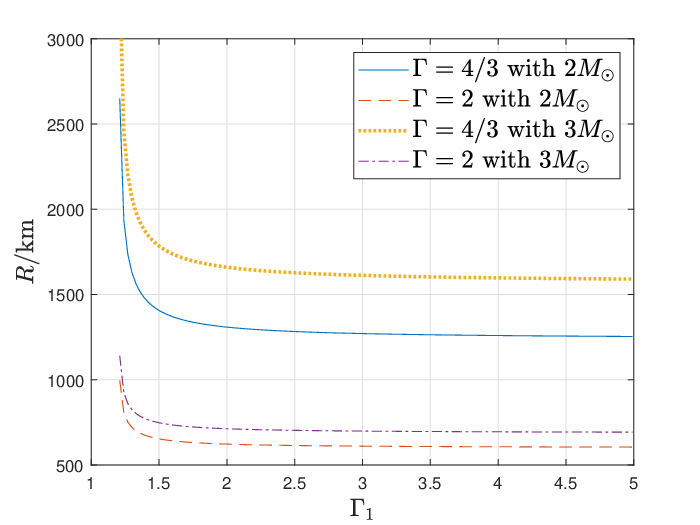
Furthermore, Figs 1, 2 and 3 with 4, 5 and 6 show that, for a given mass, with increasing there is a decrease in the star’s maximum attainable radius. This can be understood by solving equation (9) for various . However, decreasing corresponds to a significant decrease in the magnetic field, by two orders of magnitude when falls from 2 to 4/3, and this increases . So we expect that for and a star (curve A) is greater than for and a star (curve B). Figs 7 and 8 illustrate this for the Flux Conservation model and the Power Law model respectively for and stars. While curve A is always above curve B throughout for the Power Law model in Fig. 8, indicating larger radii for the former, the Flux Conservation model in Fig. 7 shows an intersection of the two curves. This is due to the fact that there is a stronger dependence in for curve A than for curve B (equations 30 and 44) and so the magnetic flux dominates at higher for curve A, thereby driving it below curve B, and hence decreasing , above a certain . Physically this may be thought of as the effect of high magnetic flux density supporting gravity.
However equation (9), and consequently equation (44), cannot be used to calculate the radius of white dwarfs with small magnetic field (G) unless the magnetic flux is fixed. For a fixed magnetic flux, decreasing field increases the radius, the information pertaining to which is missing in equation (44). More precisely, it is the dependence of radius on magnetic field in equation (44) which increases the radius extremely for small magnetic fields and this is unphysical. This is mainly because, at a lower , the contribution from thermal energy cannot be neglected compared with the magnetic energy and so equation (44) becomes invalid.
5 Conclusions
We have demonstrated the power of the highly magnetized virial theorem to make broad statements about highly magnetized stars, particularly white dwarfs. The virial theorem is generally applicable to dynamical and thermodynamic systems and can be formulated to address a plethora of other systems, including relativistic systems and stars with magnetic fields or rotation. In the presence of additional effects, the magnetic field in our case, application of the calculus of variations to the theorem can provide information about dynamical behaviour because it represents a structural relationship that the system must follow. However, we emphasize that the virial theorem is an integral theorem that generally relates scalar quantities, three different energy contributions in this case, rather than vectors. Usually this reduction in complexity results in an associated loss of information and we do not obtain as complete a description of a physical system as would be possible from a complete analysis of the system (Collins 1978). Nevertheless, we have presented simple analytical models of the properties of highly magnetized white dwarfs, wherein important properties are revealed merely by looking at the contributions of gravitational, thermal and magnetic energies. We have shown how these various contributions to energy change with the introduction of the strong magnetic field when compared to nonmagnetic or weakly magnetic counterparts. This leads us to understand the overall properties of a systems, in our case white dwarfs.
More precisely, we have explored the application of the virial theorem to recently proposed B-WDs. These highly magnetic white dwarfs can explain several observations, including peculiar over-luminous type Ia supernovae, some white dwarf pulsars, soft gamma-ray repeaters and anomalous X-ray pulsars (Mukhopadhyay & Rao 2016a), all of which have otherwise been rather puzzling. We have shown that incorporating magnetic field and thence magnetic pressure in the virial theorem can explain the existence of super-Chandrasekhar white dwarfs with radii significantly smaller than those of non-magnetized white dwarfs. We have explored this with two inherently different models: the first considers a core with constant magnetic field and a varying field in the outer envelope that conserves the magnetic flux; and the second models the magnetic pressure as varying with the matter density as a power law throughout. Flux conservation is able to explain the magnetic field variation and so the magnetic pressure variation of a B-WD as well as a non-magnetic white dwarf. Our chosen boundary conditions, which are otherwise considered realistically for white dwarfs, play an important role when we obtain the coefficients , and in the various energy contributions. Nevertheless, under certain assumptions, which include a profile that varies with the same slope for all sizes of central core, our results show that a star might retain its spherical shape in spite of the presence of strong magnetic field if it is non-rotating. Importantly while a field profile needs to be prescribed in order to obtain our results, the same results are obtained from apparently different model profiles. The only common feature is how the field varies, in one model directly with the radial coordinate and in the other with the stellar density which also falls with radius. This suggests that it is not really the model profile, but the effect of the magnetic field in general which reveals new physics in the magnetized virial theorem.
A more detailed and rigorous study of these magnetized objects would uncover more of their inconspicuous features. Nevertheless, as preliminary global estimates of strongly magnetized stellar properties, including how strong a magnetic field could be maintained in a star, this modified virial theorem serves as a very useful tool.
Acknowledgements
AS thanks the Department of Physics, Indian Institute of Science, Bangalore, for providing internships during the winters of 2017 and 2019, where most of the work was composed. CAT thanks Churchill College for his fellowship. The work is partly supported by a project of Department of Science and Technology (DST-SERB), India, with Grant No. DSTO/PPH/BMP/1946 (EMR/2017/001226). Thanks are also due to the referee for encouraging comment and suggestion to improve the presentation of the work.
Data availability
No new data were generated or analysed in support of this research. Any numerical codes and related data generated during the work will be made available whenever required by the readers.
References
- Bandyopadhyay et al. (1997) Bandyopadhyay D., Chakrabarty S., Pal S., 1997, Phys. Rev. Lett., 79, 2176
- Banerjee et al. (2017) Banerjee S., Shankar S., Singh T. P., 2017, J. Cosmol. Astropart. Phys., 2017, 004
- Belyaev et al. (2015) Belyaev V. B., Ricci P., Šimkovic F., Adam J., Tater M., Truhlík E., 2015, Nucl. Phys. A, 937, 17
- Bera & Bhattacharya (2016) Bera P., Bhattacharya D., 2016, doi:MNRAS, 465, 4026
- Bertolami & Mariji (2016) Bertolami O., Mariji H., 2016, Phys. Rev. D, 93, 104046
- Bhattacharya et al. (2018) Bhattacharya M., Mukhopadhyay B., Mukerjee S., 2018, doi:MNRAS, 477, 2705
- Carvalho et al. (2018) Carvalho G. A., Arbañil J. D. V., Marinho R. M., Malheiro M., 2018, Eur. Phys. J. C, 78, 411
- Chandrasekhar (1935) Chandrasekhar S., 1935, MNRAS, 95, 207
- Chatterjee et al. (2017) Chatterjee D., Fantina A. F., Chamel N., Novak J., Oertel M., 2017, MNRAS, 469, 95
- Coelho et al. (2014) Coelho J. G., Marinho R. M., Malheiro M., Negreiros R., Cáceres D. L., Rueda J. A., Ruffini R., 2014, ApJ, 794, 86
- Collins (1978) Collins G. W. II, 1978, Astron. Astrophys. Ser. Vol. 7, The Virial Theorem in Stellar Astrophysics. Pachart Publishing House, Tucson, p. 143
- Das & Mukhopadhyay (2012) Das U., Mukhopadhyay B., 2012, Int. J. Mod. Phys. D, 21, 1242001
- Das & Mukhopadhyay (2013) Das U., Mukhopadhyay B., 2013, Phys. Rev. Lett., 110, 071102
- Das & Mukhopadhyay (2014a) Das U., Mukhopadhyay B., 2014a, Mod. Phys. Lett. A, 29, 1450035
- Das & Mukhopadhyay (2014b) Das U., Mukhopadhyay B., 2014b, J. Cosmol. Astropart. Phys., 6, 050
- Das & Mukhopadhyay (2015) Das U., Mukhopadhyay B., 2015, J. Cosmol. Astropart. Phys., 05, 016
- Dong et al. (2014) Dong J., Zuo W., Yin P., Gu J., 2014, Phys. Rev. Lett., 112, 039001
- Eldridge & Tout (2019) Eldridge J. J., Tout C. A., 2019, The Structure and Evolution of Stars. World Scientific Publishing Europe, London
- Federbush et al. (2014) Federbush P., Luo T., Smoller J., 2014, Archive for Rational Mechanics and Analysis, 215, 611
- Fendt & Dravins ( 2000) Fendt C., Dravins D., 2000, Astron. Nachr., 321, 193
- Franzon & Schramm (2015) Franzon B., Schramm S., 2015, Phys. Rev. D, 92, 083006
- Franzon & Schramm (2017) Franzon B., Schramm S., 2017, MNRAS, 467, 4484
- Gupta et al. (2020) Gupta A., Mukhopadhyay B., Tout C. A., 2020, MNRAS, 496, 894
- Herrera & Barreto (2013) Herrera L., Barreto W., 2013, Phys. Rev. D, 87, 087303
- Howell et al. (2006) Howell D. A., et al., 2006, Nature, 443, 308
- Kalita & Mukhopadhyay (2019) Kalita S., Mukhopadhyay B., 2019, MNRAS, 490, 2692
- Kalita et al. (2020) Kalita S., Mukhopadhyay B., Mondal T., Bulik T., 2020, ApJ, 896, 69
- Kundu & Mukhopadhyay (2012) Kundu A., Mukhopadhyay B., 2012, Mod. Phys. Lett. A, 27, 1250084
- Liu et al. (2014) Liu H., Zhang X., Wen D., 2014, Phys. Rev. D, 89, 104043
- Markey & Tayler (1973) Markey P., Tayler R. J., 1973, MNRAS, 163, 77
- Moussa (2017) Moussa M., 2017, Annals of Physics, 385, 347
- Mukhopadhyay & Rao (2016a) Mukhopadhyay B., Rao A. R., 2016, J. Cosmol. Astropart. Phys., 5, 007
- Mukhopadhyay et al. (2016) Mukhopadhyay B., Das U., Rao A. R., Subramanian S., Bhattacharya M., Mukerjee S., Bhatia T. S., Sutradhar J., 2017, in Tremblay P.-E., Gänsicke B., Marsh T., eds, Astronomical Society of the Pacific Conference Series Vol. 509, 20th European White Dwarf Workshop. Astron. Soc. Pac., San Francisco, p. 401
- Mukhopadhyay et al. (2017) Mukhopadhyay B., Rao A. R., Bhatia, T. S., 2017, MNRAS, 472, 3564
- Narayan & Yi (1994) Narayan R., Yi I., 1994, ApJ, 428, L13
- Ostriker & Hartwick (1968) Ostriker J. P., Hartwick F. D. A., 1968, ApJ, 153, 797
- Otoniel et al. (2019) Otoniel E., Franzon B., Carvalho G. A., Malheiro M., Schramm S., Weber F., 2019, ApJ, 879, 46
- Eslam Panah & Liu (2019) Eslam Panah B. E., Liu H., 2019, Phys. Rev. D, 99, 104074
- Pili et al. (2014) Pili A. G., Bucciantini N., Del Zanna L., 2014, MNRAS, 439, 3541
- Pons & Viganó (2019) Pons J. A., Viganó D., 2019, Liv. Rev. Com. Astrophys., 5, 3
- Quentin & Tout (2018) Quentin L. G., Tout C. A., 2018, MNRAS, 477, 2298
- Roy et al. (2019) Roy S. K., Mukhopadhyay S., Lahiri J., Basu D., 2019, Phys. Rev. D, 100, 063008
- Scalzo et al. (2010) Scalzo R. A., et al., 2010, ApJ, 713, 1073
- Shah & Sebastian (2017) Shah H., Sebastian K., 2017, ApJ, 843, 131
- Shapiro & Teukolsky (1983) Shapiro S. L., Teukolsky S. A., 1983, Black Holes, White Dwarfs and Neutron Stars: The Physics of Compact Objects. Wiley, New York
- Sotani & Tatsumi (2017) Sotani H., Tatsumi T., 2017, MNRAS, 467, 1249
- Subramanian & Mukhopadhyay (2015) Subramanian S., Mukhopadhyay B., 2015, MNRAS, 454, 752
- Tayler (1973) Tayler R. J., 1973, MNRAS, 161, 365
- Wickramasinghe et al. (2013) Wickramasinghe D. T., Tout C. A., Ferrario L., 2013, MNRAS, 437, 675