Adaptive Subcarrier, Parameter, and Power Allocation for Partitioned Edge Learning Over Broadband Channels
Abstract
In this paper, we consider partitioned edge learning (PARTEL), which implements parameter-server training, a well known distributed learning method, in a wireless network. Thereby, PARTEL leverages distributed computation resources at edge devices to train a large-scale artificial intelligence (AI) model by dynamically partitioning the model into parametric blocks for separated updating at devices. Targeting broadband channels, we consider the joint control of parameter allocation, sub-channel allocation, and transmission power to improve the performance of PARTEL. Specifically, the policies for joint SUbcarrier, Parameter, and POweR allocaTion (SUPPORT) are optimized under the criterion of minimum learning latency. Two cases are considered. First, for the case of decomposable models (e.g., logistic regression), the latency-minimization problem is a mixed-integer program and non-convex. Due to its intractability, we develop a practical solution by integer relaxation and transforming it into an equivalent convex problem of model size maximization under a latency constraint. Thereby, a low-complexity algorithm is designed to compute the SUPPORT policy. Second, consider the case of deep neural network (DNN) models which can be trained using PARTEL by introducing some auxiliary variables. This, however, introduces constraints on model partitioning reducing the granularity of parameter allocation. The preceding policy is extended to DNN models by applying the proposed techniques of load rounding and proportional adjustment to rein in latency expansion caused by the load granularity constraints.
I Introduction
Edge machine learning is an area concerning the deployment of learning algorithms at the network edge to gain low-latency access to data and computation resources distributed at a large number of edge devices [1]. In this work, we study the efficient implementation of the well-known method of parameter-server training [2] in a broadband system (e.g., 3GPP 5G) to exploit distributed computation resources at many devices to scale up model training. To this end, several key operations, namely computation-load allocation (via model partitioning), sub-channel allocation, and power control, are jointly designed under the criterion of minimum learning latency.
Two main methods for distributed learning are federated learning [3, 4] and parameter-server training [2, 5, 6], which are designed for different scenarios and features. The key feature of federated learning is its preservation of data privacy. Based on distributed implementation of stochastic gradient descent (SGD), federated learning iterates the separate training of a downloaded model at multiple devices using their local data, and the uploading and aggregation of local models (or local stochastic gradients) to yield a more accurate global model [3, 4]. The avoidance of direct data uploading protects their privacy. Though it is similar to federated learning in implementing distributed SGD, the parameter-server training, which is of our interest, has one distinction. Its purpose is to scale up learning using many resource-constrained machines in a closed network where data privacy is not a concern [2]. To this end, the model is partitioned to allow each device to train only a part of the model instead of the whole as in federated learning. This overcomes the resource constraints of devices and reduces their energy consumption. Moreover, training data are downloaded from a server to devices at the beginning of each round, avoiding their need of persistent storage space.
A current main theme in the field of edge learning is the design of wireless techniques to support efficient deployment of federated learning, resulting in an area called federated edge learning (FEEL) [7]. The effort on overcoming the communication bottleneck of FEEL has led to the design of a new class of multi-access techniques realizing over-the-air model aggregation[8, 9, 10, 11, 12] and radio resource management (RRM) techniques [13, 14, 15, 16, 17]. Moreover, researchers have designed energy efficient RRM techniques to tackle the challenge of executing a complex learning task at energy constrained devices in a FEEL system[18, 19, 20]. Recently, researchers have also explored the efficient implementation of parameter-server training over wireless channels, resulting in a framework called partitioned edge learning (PARTEL) [21]. Let parameter allocation refers to the system operation that to balance computation loads, the server divides the model into parametric blocks of variable lengths and allocate them to devices for separate training. To reduce the learning latency, the technique of joint parameter allocation and resource allocation is proposed in [21], which jointly adapts parameter and bandwidth allocation to devices’ channel states and computation capacities. For simplicity, the prior work assumes narrowband channels, for which the management of uplink radio resource reduces to bandwidth allocation. In this work, we design low-latency PARTEL techniques for a broadband system (e.g., 3GPP 5G) with frequency selective channels. In this case, the frequency resource is managed via sub-channel allocation, which is much more complex than bandwidth allocation. The complexity arises from the fact that the sub-channels of each device have different gains and devices have different channel realizations. Consequently, even if the allocated bandwidths are fixed, reshuffling the assignments of sub-channels varies devices’ communication rates. Therefore, jointly designing sub-channel and parameter allocation poses a new challenge that cannot be tackled using the solution in [21].
The optimal sub-channel allocation is well known to be an integer optimization problem that is NP hard [22, 23, 24]. For the conventional multiuser communication systems, the classic approximate-solution approach has been established in a series of work for the purpose of minimizing sum power under users’ rate constraints [22, 23, 24]. The essential idea is to relax the integer program and discover the embedded convexity in the relaxed problem to design a practical algorithm [22]. In this work, we build on the classic approach to develop a new solution for the problem of latency minimization in a broadband PARTEL system. The distinction of the current work is the pursuit of a communication-learning integration approach so as to minmize learning latency in the context of PAETEL. To this end, we jointly design parameter and sub-channel allocations. The considerations of synchronized updates by devices, which is a requirement for parameter-server training [2], and devices’ heterogeneous computation capacities introduce more challenges. Existing designs that aim at generic radio access cannot tackle the new challenges, which motivate the current work.
It is also worth mentioning that we also consider a more complex model based on a deep neural network (DNN) besides the decomposable model as in [21]. Unlike the latter, the former is not directly decomposable and requires the modification of learning algorithm to support PARTEL. This introduces additional complexity to the current design.
By tackling the above challenges, we design a set of algorithms for joint SUbcarrier, Parameter, POweR allocaTion (SUPPORT), termed joint SUPPORT. The main contributions of this work are summarized as follows.
- •
Joint SUPPORT for Decomposable Models: Consider the case of a decomposable model. The problem of latency minimization by joint SUPPORT is an integer program and intractable. A practical solution approach is developed using two techniques. The first is a relaxation of binary subcarrier assignment decisions. The second is the transformation of the relaxed problem into a convex problem of model size maximization under a latency constraint, which is nested in a simple search for the target model size. Considering the convex problem, the properties of three optimal resource-management operations are analyzed and then applied to design an efficient algorithm for computing the desired SUPPORT policy. Via analysis, it is found that the optimal number of parameters assigned to a worker for updating avoids high power consumption due to overloading. For this reason, the optimal number is derived to be a concave function of its speed and a monotonic decreasing function of its computation power factor. On the other hand, the optimal subcarrier assignment and power allocation over assigned subcarriers are found to favor high channel gains.
- •
Joint SUPPORT for DNN Models: Consider the case of a DNN model. The optimization problems for joint SUPPORT in both mini-rounds are shown to have the same form as that in the preceding case except for additional load granularity constraints. This allows the extension of the joint SUPPORT policy for the case of decomposable models to the current case by rounding down the obtained loads to meet the granularity constraints. Furthermore, the remaining parameters due to rounding are allocated over devices and subcarriers proportionally with their rounded loads, thereby reining in the latency expansion caused by the additional constraints.
The performance gain of the above algorithms and the findings are corroborated using experiments with a real dataset.
The reminder of the paper is organized as follows. In Section II, the system model is introduced. In Section III, the total learning latency minimization problem is formulated. In Section IV and V, the joint SUPPORT designs are proposed for decomposable models and DNN models, respectively. Section VI presents the experimental results followed by concluding remarks in Section VII.
II Models and Metrics
II-A System Model
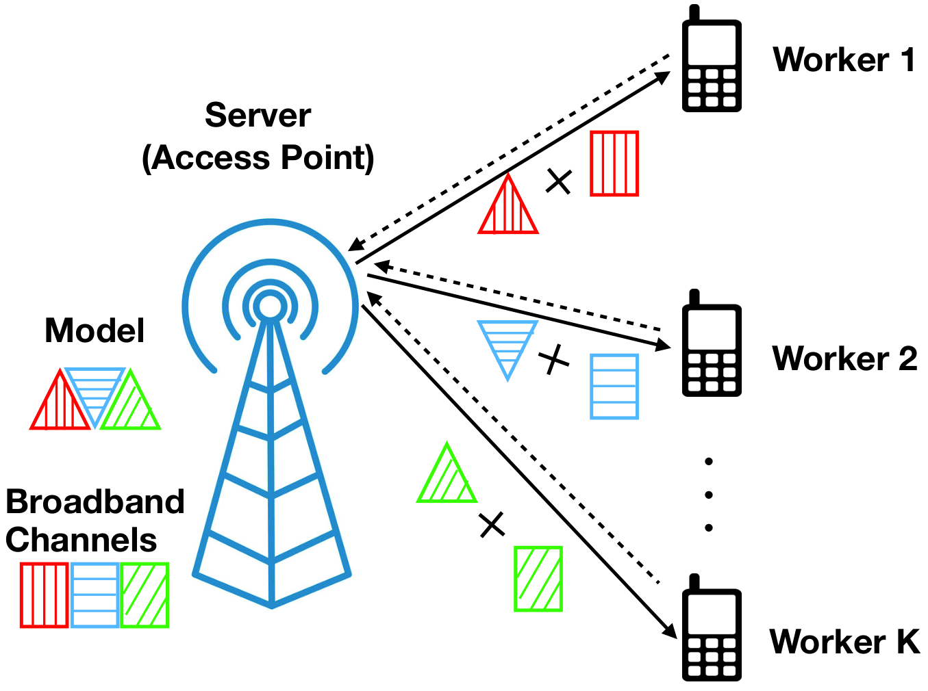
A single cell OFDM system is considered, as illustrated in Fig. 1(a). In the cell, there are one server equipped with a single-antenna access point (AP) and single-antenna edge devices, serving as workers. Each worker performs one task assigned by the server. The server is connected to workers via wireless links. The system bandwidth is divided into orthogonal subcarriers. The bandwidth of each subcarrier is denoted as . The frequency-selective fading channel is considered, where different subcarriers will experience different channel gains. We assume that the AP has the channel state information (CSI) of all links that are useful for subcarrier allocation. Besides, the channel gains are assumed to be static in one training iteration but vary over different iterations. The uplink channel gain of worker on the subcarrier is denoted as . We denote as the subcarrier allocation indicators. If the -th subscriber is allocated to worker , then . Otherwise, .
II-B Learning Models
II-B1 Decomposable Models
The large-scale learning tasks with decomposable objective functions (such as logistic regression) can be directly implemented using PARTEL based on the method of block coordinate descent. According to the literature (e.g., [21]), a decomposable objective function can be written as
| (1) |
where is the parameter vector of the learning model, is the size of , is the loss function, and is the regularized function (e.g., regularization used to increase sparsity and regularization used to reduce overfitting). Specifically, the loss function can be written as , where is the size of the dataset, is the -th data sample, and is a smooth inference function. The regularized function is a block-separable function, given as , where is the -th element of and is the norm (e.g., or norm). During the training, the smoothness of decides the method to update the learning model. If is smooth, gradient descent algorithm is used. Otherwise, another method called proximal gradient descent, is used.
II-B2 DNN Models
DNN models cannot be directly implemented using PARTEL, as the nested layers therein make the gradient elements of different layers dependent. To make PARTEL feasible and efficient for DNNs, in the sequel, the method of auxiliary variables is used to decompose the DNN models into many independent subproblems [5, 6].
First, consider a DNN model with hidden layers. The model parameter matrix is denoted as with the size of parameters. For an arbitrary layer therein, say layer , the parameter matrix is denoted as , the number of neurons is denoted as , and the -th neuron parametric vector is denoted as . Thereby, the objective function of the DNN model is given by
| (2) | ||||
where the model parameter matrix can be expressed as , the parameter matrix of the -th layer can be expressed as , and is the set of output (activation) functions of the -th layer.
Auxiliary Variables: The method of auxiliary variables is used by introducing one auxiliary variable per neuron per data sample: , where is the activation function, is the -th neuron parametric vector in layer , is the auxiliary variable introduced for the -th neuron in layer regarding data sample , is the auxiliary variable vector for the layer regarding data sample , and is the number of neurons in the -th layer. For an arbitrary data sample, say the -th, the corresponding auxiliary matrix for the whole model is denoted as , called per-sample auxiliary matrix. Then the overall auxiliary matrix for all samples are denoted as .
Decomposed Optimization: Following [5, 6], by using the quadratic-penalty method, the problem in (2) is equivalent to minimizing
| (3) |
where and . In (3), the nested structure among layers is decoupled. Consequently, the gradients of any two parameters (or auxiliary variables) are independent.
Finally, the problem in (3) can be solved using the alternating optimization over and , i.e., sequentially solving the -stage and -stage, defined below, in each training iteration.
- •
-stage: Fixing the values of , solve the problem of , in which the problem of each neuron is independent and can be written as
(4) where and are the parameteric vector and auxiliary variable of the -th neuron in the -th layer, respectively, is the auxiliary variable vector of the -th layer. Note that one device is allocated a task of updating one or more neuron parametric vectors by solving the subproblems in (4).
- •
-stage: Conditioned on the values of , solve the problem of , where the problem of optimizing each per-sample auxiliary matrix is independent of others and is given as
(5) where is the per-sample auxiliary matrix corresponding to data sample . The size of the per-sample auxiliary matrix is with being the number of neurons in layer . Note that one device is allocated a task of updating one or more per-sample auxiliary matrices by solving the subproblems in (5).
II-C PARTEL Architecture
Consider the PARTEL system and operations in Fig. 1, that are elaborated as follows.
II-C1 Decomposable Models
The model-parameter vector is partitioned into disjoint parametric blocks, as , where is allocated to worker for update, using a downloaded global dataset from the server11 1 The joint SUPPORT design of this paper can be easily extended to the case of partitioned dataset with multiple groups of workers (each with a data subset). Each group cooperatively updates a same block. The proposed joint SUPPORT can be applied in a hierarchical manner: applied for inter-group resource management and also applied for intra-group management.. The communication overhead for the server to broadcast the dataset is ignored, as its large power and bandwidth are used and the dataset broadcasting requires only once before the model training. One main benefit of PARTEL is low learning latency, as each resource-constrained worker is required to calculate and transmit the gradient or proximal gradient of only a parametric block instead of the whole parameter vector during each iteration [21].
In the PARTEL framework, one training iteration of the decomposable models is called one (communication) round. As shown in Fig. 1(b), there are three phases in each round, as follows.
- •
Push Phase: The server broadcasts the whole model-parameter vector, , to all workers.
- •
Computation Phase: Each worker computes the update (e.g., gradients or proximal gradients) of its allocated parametric block.
- •
Pull Phase: All workers upload the updates of their corresponding parametric blocks to the server. The server updates the whole parameter vector.
The training process in Fig. 1(b) iterates when all parametric blocks are updated in the round, i.e., the tasks of all workers are synchronized in each round.
II-C2 DNN Models
As mentioned, each round of DNN models comprises two stages: -stage and -stage, described as follows.
- •
-stage: The parameter matrix is divided into blocks, with each being updated by one worker. To avoid inter-communication among different workers, the following load-granularity constraint is applied.
Granularity Constraint 1 (Neuron Allocation for -stage).
In -stage, each neuron parametric vector (e.g., ) defined in (4) should be allocated to one and only one worker.
- •
-stage: The auxiliary matrix is divided into blocks, with each being updated by one worker. To avoid inter-communication among workers, another load-granularity constraint is applied.
Granularity Constraint 2 (Per-Sample Auxiliary Matrix Allocation for -stage).
In -stage, each per-sample auxiliary matrix (e.g., ) defined in (5) should be allocated to one and only one worker.
Example 1.
Since the number of neurons in a DNN model and the data samples used for training are large, the sizes of each neuron problem and each per-sample auxiliary matrix problem are relatively small, compared with the whole learning tasks, making the model partitioning meaningful. As an example, our experiments involve the DNN model “Lenet-5” proposed in [25] trained on the MNIST dataset. A mini batch of samples is used in each training iteration. In “Lenet-5”, there are 3 convolutional layers, including feature maps in total. The first two convolutional layers are followed by a pooling layer and the last is followed by a fully connected layer with neurons. In -stage, the number of independent subproblems is . The size of each neuron problem is about of the whole problem. In -stage, the size of each per-sample auxiliary matrix problem is of the whole problem.
Each stage (-stage or -stage) comprises three phases, push, computation, and pull, which are similar to those in the case of decomposable models. The main difference lies in the additional Granularity Constraint 1 or 2. Each round comprises two stages and the rounds are repeated until the DNN model converges.
II-D Latency and Energy Consumption Models
Consider an arbitrary communication round and an arbitrary worker, say worker . The latency and energy consumption models of each phase are described as below.
II-D1 Push Phase
The push latency is the time for the server to broadcast the whole model-parameter vector to all workers. It is a constant identical for all workers. Besides, as the transmit power and bandwidth are very large during broadcasting, the push latency can be ignored. In this step, the energy consumption by all workers is to receive the model-parameter vector from the server and is included in the circuit energy consumption, denoted as .
II-D2 Computation Phase
The computation latency of worker depends on the size of the allocated parametric block and its computation speed :
| (6) |
where is measured by the number of parameters processed per second.
According to [26], the computation power of worker is , where is the computation power factor. Then, the computation energy of worker is
| (7) |
II-D3 Pull Phase
The pull phase consists of two parts. One is uploading gradient blocks from workers to the server. The other is the server updating the global model using the gradients sent by the workers. For the latter part, there is no energy consumption at the workers. Its latency, denoted as , is a constant and is same for all workers. In the sequel, we ignore the model update latency, , as it is small and has no impact on the solution of latency minimization.
For uploading, worker transmits over a set of assigned subcarriers. We denote as the uploading latency of worker on subcarrier . If subcarrier is not allocated to , i.e., , . Otherwise,
| (8) |
where is the number of parameters uploaded by worker on subcarrier , is the number of bits per gradient element, and is the channel capacity of worker on subcarrier . The channel capacity is given by , where is the subcarrier bandwidth, is the power of additive white Gaussian noise, is the transmit power, and is the channel gain of worker on subcarrier , respectively. It follows that
| (9) |
Then, the overall uploading latency of worker is decided by the slowest subcarrier:
| (10) |
The uploading energy consumption of worker is modeled as follows. Let denote the transmit energy consumption of worker on subcarrier . If subcarrier is not allocated, i.e., , . Otherwise,
| (11) |
By substituting the transmit power density in (9) and the uploading latency in (8), can be further derived as
| (12) |
The total uploading energy consumption of worker is the sum of uploading energy consumption over all subcarriers: . By substituting in (12),
| (13) |
Next, the total latency and energy consumption of worker are defined as follows. The latency of worker is the sum latencies of the two phases:
| (14) |
where is the computation latency defined in (6), is the uploading latency defined in (10). The energy consumption of worker is given by:
| (15) |
where is the constant circuit energy consumption when there is no computation and transmission, defined in (7) and defined in (13) are the computation and uploading energy consumption of worker , respectively.
III Problem Formulation
We aim at minimizing the overall learning latency of the PARTEL system, which depends on two factors: the per-round latency and the number of rounds for model convergence. The overall learning latency is defined as the total latency of all rounds till model convergence. In [21] for narrowband channels, it is proved that the overall learning latency minimization is equivalent to separately minimizing the per-round latency. The result can also apply to the current case of broadband channels, as stated below.
Lemma 1 (Equivalent Per-Round Latency Minimization [21]).
The overall learning latency minimization is equivalent to separately minimizing the latencies for all rounds.
Lemma 1 holds because the distributed learning algorithms implemented using PARTEL are equivalent to the corresponding centralized ones in terms of convergence rate as measured by the required number of communication rounds. Specifically, for distributed learning, the values of updates (e.g., gradients and proximal gradients) calculated in each round and the number of rounds required for model convergence are independent of SUPPORT.
Using the result in Lemma 1, we formulate the equivalent per-round latency-minimization problem. For an arbitrary round, we aim to minimize its latency, denoted as , under the constraints on subcarrier assignment, latency requirement, parameter allocation, and power control, described as follows.
III-1 Subcarrier Assignment Constraints
Each subcarrier can be allocated to one worker:
| (16) |
where represents that the subcarrier is allocated to worker .
III-2 Per-Round Latency Constraints
As all parametric blocks should be updated in one round, all workers’ latencies, say , should not exceed the overall one-round latency :
| (17) |
As mentioned, is the latency for an arbitrary round and can be different over different rounds. By substituting in (14), the constraints in (17) can be derived as
| (18) |
which, by substituting the uploading latency in (10), are equivalent to
| (19) |
where defined in (6) is the computation latency of worker and defined in (8) is the uploading latency of worker on subcarrier .
III-3 Parameter Constraints
The parameter constraints are two tiers. On the one hand, the total updatable number of parameters by all workers should be no smaller than the size of the model:
| (20) |
where is the size of the parametric block allocated to worker and is the size of the model-parameter vector (or matrix). On the other hand, for each worker, the total uploaded number of parameters on all subcarriers should be no smaller than its allocated parametric-block size:
| (21) |
where is the number of parameters uploaded by worker on subcarrier . In the sequel, and are relaxed to be continuous for simplicity. In practice, the solved and will be rounded for implementation and the loss caused by the rounding operation can be ignored, since the values of and are typically large.
For the case of DNN models, Granularity Constraints 1 and 2 can be written mathematically as follows.
| (22) |
where is the set of positive integers and is the size of the subproblems, i.e., neurons or per-sample auxiliary matrices. For -stage, the size of all neurons, say , are assumed the same for simplicity, which has little impact on the solution, since the size of each neuron is much smaller than that of the whole problem, as mentioned in Example 1. For -stage, the size of each per-sample auxiliary matrix is the total number of neurons, say with being the number of neurons in layer .
III-4 Power Constraints
III-5 Latency-Minimization Problem
Under these constraints, the per-round latency-minimization problem by joint SUPPORT can be formulated as
| (24) |
IV Joint SUPPORT for Decomposable Models
In this section, joint SUPPORT is designed by developing a tractable approach for solving Problem (P1).
IV-A Equivalent Latency Requirement
First, the following necessary condition for the equivalent latency requirement can be derived to simplify Problem (P1). Note that in [21], similar equivalent latency property can be derived in the PARTEL design for frequency non-selective channels. However, for OFDM systems considered in this paper, the binary subcarrier allocation among workers and the corresponding inter-subcarrier power and parameter allocation for each device make the problem much more complicated.
Lemma 2 (Equivalent Latency for All Workers).
Proof: See Appendix -A.
The result in Lemma 2 yields the following insights. First, it requires all workers the same latency with the overall latency . Second, for each worker, the uploading latency on all allocated subcarriers should be equal.
Remark 1 (Computation Latency vs. Communication Latency).
By substituting the computation latency in (6) and the communication latency in (8) into the equivalent latency property in (25), it can be derived as
| (26) |
with the constraints . From (26), the load, say , has the same effect on computation and communication latency. On the other hand, when the computation frequency is small compared to the number of subcarriers and the data rates, the computation latency dominates or vice versa.
By substituting the computation latency defined in (6) and the uploading latency defined in (8) into the necessary condition in Lemma 2, we can derive the number of parameters uploaded by worker on subcarrier , say , as
| (27) |
where is the per-round latency, is the subcarrier-allocation indicator, is the parametric-block size allocated to worker , is the channel capacity of on subcarrier . By substituting defined in (27) and the necessary condition in Lemma 2, Problem (P1) can be simplified as:
| (28) |
where defined in (15) is the energy consumption of worker . By substituting in (27), can be expressed as
| (29) |
IV-B Equivalent Convex Problem
Problem (P2) is a mixed integer non-convex problem and is hence NP-hard [27]. In the sequel, two steps are used to tackle it. First, following the standard approach to tackle integer programming (see e.g., [22]), linear programming relaxation is used to relax the subcarrier-allocation indicators in Problem (P2) to be continuous, i.e., . Then, following the method in [21], the relaxed problem can be equivalently converted to the problem of updatable model size maximization. However, it remains non-convex and difficult to tackle due to the intra-worker parameter constraint and the power constraint. In the sequel, the problem of updatable model size maximization is derived and solved.
Given the one-round latency for an arbitrary round, let denote the maximum size of a model that can be updated within the round. Then solves the following problem of model size maximization:
| (30) |
where is the subcarrier-allocation indicator, is the parametric-block size allocated to worker , is the channel capacity of worker on subcarrier , is the one-round latency, defined in (29) is the energy consumption of worker . Note that solving Problem (P2) via utilizing the problem of model size maximization in Problem (P3) follows the method in [21]. However, new challenges arise from the subcarrier allocation among workers and the inter-subcarrier power and parameter allocation for each worker, leading to the non-convexity and a much larger size of Problem (P3).
Lemma 3 (Relation of Maximal Model Size and Latency).
defined in Problem (P3) is a monotonously increasing function of .
Proof: See Appendix -B.
It follows from the result in Lemma 3 that the solution of Problem (P2) is the minimal latency, say , which makes the updatable model size no less than the target size . This suggests a method to solve Problem (P2) by searching using the criterion , which will be elaborated in the later subsection.
To get the maximum updatable model size requires solving Problem (P3). To this end, the following variables are used to transform Problem (P3) into a convex problem.
| (31) |
By substituting the variables in (31) and defined in (29), Problem (P3) can be written as
Lemma 4.
Problem (P4) is a convex problem.
Proof: See Appendix -C.
IV-C Properties of Optimal Policies
Based on the results in the previous subsection, the optimal policies of Problem (P2) with relaxed subcarrier-allocation indicators are proposed, as described in the following.
As (P4) is convex, the primal-dual method can be used to get the optimal solution:
| (32) |
where is the Lagrange function of Problem (P4), given as
| (33) | ||||
and , , and are Lagrangian multipliers.
Next, the necessary conditions for achieving the optimal solution of the inner loop are used to derive the optimal policies. The inner loop problem is given by
| (34) |
The first necessary condition is
| (35) |
which gives the following optimal scheme for calculating the channel capacity:
| (36) |
By substituting in (36) into the transmission power in (9), the optimal power-allocation scheme can be derived, as in the following lemma.
Lemma 5 (Optimal Power Allocation).
The optimal power-allocation scheme is
| (37) |
The water-filling like result in (37) shows that for each worker, more power should be allocated on the subcarrier with high channel gain, say .
The second necessary condition to achieve the optimum of the inner loop problem in (34) is
| (38) |
By substituting the variable transformations in (31) into (38), we can achieve the optimal inter-worker parameter allocation scheme, as follows.
Lemma 6 (Optimal Parameter Allocation among Workers).
The optimal inter-worker parameter-allocation scheme is
| (39) |
In (39), the optimal parametric-block size allocated to worker , say , is a concave function of the computation speed and a monotone decreasing function of the computation power factor . On one hand, large can reduce the computation latency. On the other hand, the computation energy increases as a square function of . The optimal load in (39) balances the two aspects.
Substituting the parameter-allocation scheme in (39) and the channel capacity in (36) into the intra-worker parameter-allocation scheme in (27), gives the following lemma.
Lemma 7 (Optimal Parameter Allocation Among Subcarriers).
The optimal intra-worker parameter allocation scheme is given by
| (40) |
From (40), more parameters should be assigned to the channel with high gain.
The third necessary condition to achieve the optimum of the inner loop problem in (34) is
| (41) |
where is the indicator function given by
| (42) |
Note that is determined when is known. Let . If , , as the condition in (41) can not be satisfied. If for a unique worker, say , then . If for multiple workers, then for these workers. And in the last case, it is easy to show that the values of the non-zero won’t influence the value of the Lagrange function defined in (33), as long as the subcarrier assignment constraint, say , are satisfied.
The optimal subcarrier allocation is summarized in the following lemma.
Lemma 8 (Optimal Subcarrier Allocation).
In (43), a high channel gain leads to a small value of and thus a high possibility to make . That means the subcarrier with higher channel gain has larger possibility to be allocated to the worker. Note that in the optimal scheme in Lemma 8, some subcarrier-allocation indicators may be fractions. The standard approach is to round those to be binary (see, e.g., [22]), which will be elaborated in the later subsection.
IV-D Optimal Policy Computation
In this subsection, the joint SUPPORT algorithm to solve the original Problem (P1) is proposed. First, we solve the convex Problem (P4) by the primal-dual method using the closed-form results in Lemmas 6-8. Some notation is described as follows. and denote the step sizes of gradient descent. and , , and are the Lagrange function and Lagrangian multipliers defined in (33). With the notation, the application of the primal-dual method yields Algorithm 1 for solving Problem (P4).
Remark 2 (Low Complexity of Updatable Model Size Maximization).
The computation complexity of Algorithm 1 is with being the number of workers and being the number of subcarriers, as the closed-form results in Lemmas 6 - 8 makes the updating of corresponding variables more efficient. As a comparison, directly solving the non-convex Problem (P3) has a computational complexity of at least and is suboptimal.
1: Input: channel gains , computation speeds , computation power factors, , and the given one-round latency .
2: Initialize , , and .
3: Loop
4: Update the multipliers as
6: Get and with (31).
7: Until Convergence
8: .
9: Output: , , , and .
Then, as mentioned in the preceding subsection, Problem (P2) with relaxed subcarrier-allocation indicators can be solved by nesting a one-dimensional search over the latency and solving the convex Problem (P4). Based on the monotonicity of in Lemma 3, the search can be efficiently implemented by bisection method. While the solution of Problem (P4) is presented in Algorithm 1. Then the optimal policy to solve Problem (P2) with relaxed subcarrier-allocation indicators is presented in Algorithm 2, by nesting the bisection search and Algorithm 1.
1: Input: channel gains , computation speeds , and computation power factors, .
2: Select that makes defined in Problem (P4) larger than .
3: Select that makes .
4: While
5: Let .
6: Input , , and into Algorithm 1 to solve (P4).
7: Obtain , , , and .
8: If
9: .
10: Else
11: .
12: End if
13:End while
14:.
15:Output: , , , and .
Finally, based on Algorithm 2, the joint scheme of SUPPORT without relaxation is proposed to solve the original Problem (P1). Note that not all subcarrier-allocation indicators solved by Algorithm 2 are integers, i.e., for some . For these subcarriers, a practical subcarrier-allocation scheme following [22] is determined as
| (44) |
where the subcarrier is allocated to the worker with the largest value. Then, given the subcarrier-allocation scheme , the latency-minimization problem is a special case of Problem (P1), whose solution can also be solved by Algorithm 2.
V Joint SUPPORT for DNN Models
In this section, DNN models are considered. Since Problem (P1) is not tractable in this case with the additional constraint (), we propose an approximate solution method that leverages the result for decomposable model case, described as follows.
- 1.
- 2.
The challenges lie in Step 2) and are two-fold. On one hand, how should the rounding indicator be designed to minimize the rounding loss. On the other hand, as each worker’s number of parameters changes, the corresponding channel-capacity (or power) allocation and intra-worker parameter allocation among the assigned subcarriers should be redesigned. To tackle these challenges, in the sequel, we first propose a joint scheme of SUPPORT for DNN models. Then, the rounding scheme is designed accordingly and the resultant latency increase is analyzed.
V-1 Joint SUPPORT for DNN Models
Denote the solved one-round latency as , the subcarrier-allocation policy as , the spectrum efficiencies as , the number of parameters of worker as , the number of parameters uploaded by worker on subcarrier as .
Consider an arbitrary worker, say worker . If its number of parameters is rounded down to satisfy (), the reduced number of parameters is denoted as . If its number of parameters is rounded up, the additional number of parameters to be uploaded is denoted as . Note that if worker ’s number of parameters is rounded down, no influence is caused to the one-round latency. Hence, only the case of being rounded up is considered in the sequel. Our aim is to design rounding scheme to minimize the resulted additional one-round latency.
Next, the joint scheme of SUPPORT is designed as
| (45) |
where is the number of additional parameters allocated to subcarrier for uploading, which is proportional to its currently uploaded number of parameters . In (45), the allocation of subcarriers and the channel capacities of the assigned subcarriers remain the same. Two concerns motivate us to design the joint SUPPORT scheme as (45). First, the assigned subcarrier that can currently upload more updates of parameters can upload more additional parameters in the same additional latency. Second, the proportional additional parameter allocation together with the unchanged allocation of subcarriers and channel capacities can yield a simple upper bound of the additional latency for each worker, as shown in the following lemma.
Lemma 9 (Additional Latency).
Consider an arbitrary worker, say worker , the design in (45) results in an upper bound of the minimum additional latency:
| (46) |
where is the solved latency in Step 1), , , and are the additional latency, the number of additional parameters after the rounding operation, and the solved number of parameters in Step 1) of worker , respectively.
The proof of Lemma 9 is straightforward and hence omitted. Two observations can be made from Lemma 9. On one hand, as mentioned in Example 1, the size of the subproblems are far smaller than the problems of -stage and -stage, i.e., . Therefore, the additional latency is small for all workers. On the other hand, the round-up indicator, denoted as , should be the ratio .
V-2 Parameter Rounding Scheme
Note that Lemma 9 only gives the additional latency for one worker. To minimize the additional one-round latency, the rounding scheme is designed to make the workers with least to round up and the others to round down, described as follows.
- 1.
Sort the round-up indicators from the least to the biggest and the new permutation is indexed by , i.e., is sorted from the least to the largest.
- 2.
Find the least following the new permutation , which satisfies
(47) where is the additional number of parameters of worker when being rounded up and is the reduced number of parameters when being rounded down. (47) means that by rounding up workers with least round-up indicators, the parameters of all workers can satisfy Granularity Constraints 1 and 2.
- 3.
VI Experimental Results
VI-A Experiment Setup
The experimental settings are specified as follows unless specified otherwise. In the OFDM based PARTEL system, there are workers and subcarriers. The bandwidth of each subcarrier is kHz. The subcarrier channel gains are assumed to be i.i.d. Rayleigh fading with the average path loss of . The noise power density is set as W/Hz. The workers’ computation speeds are uniformly selected from the set parameters processed per second in one local computation iteration. The corresponding computation power factors are uniformly selected from the set . The maximum power consumed by workers is set as W. Both decomposable models and DNN models are trained using the PARTEL framework. The learning settings are as follows.
- •
Decomposable Model: A -regularized logistic regression task is considered, which trains a news-filtering model using the News20 dataset collected in [28]. The model size is . The training and test datasets have and samples respectively. workers with subcarriers are used to complete the task.
- •
DNN Model: The CNN model “LeNet-5” proposed in [25] is trained on the MNIST dataset. In the “LeNet-5” model, there are are parameters in total. The method of auxiliary variables in [6] is used to train the “LeNet-5” model at the PARTEL framework. In each training iteration, a mini batch of data samples is used. There are auxiliary variables in total. workers with subcarriers are used to complete the task.
For comparison, three communication schemes are considered, described as follows.
- •
Joint SUPPORT: The joint schemes of SUPPORT proposed in Sections IV or V.
- •
Baseline: The number of parameters computed by each worker is first allocated proportional to their computation capacity. Then, the subcarriers are allocated, which is a special case of the joint SUPPORT scheme.
- •
Greedy Scheme for FEEL: The training samples are equally distributed among workers. Thereby, the computation latency and energy of each worker is determined. The subcarrier allocation follows a greedy way. The subcarriers are randomly indexed and sequentially allocated from the st to the -th. The -th subcarrier is allocated to the worker whose latency is currently the longest. Note that the latency minimization of one worker given the subcarrier allocation is simple and omitted.
VI-B Decomposable Models
The learning performance of training the logistic regression model is compared in Fig. 2. As observed, the model trained in PARTEL with the proposed joint SUPPORT converges much faster than the one trained in FEEL with the greedy communication scheme, in which each worker uploads the updates of all parameters. Besides, the joint SUPPORT outperforms the baseline in terms of model convergence with a latency reduction of 31.06% on average. That’s because the allocations of parameters and subcarriers are sequentially designed in the baseline.
Fig. 3 shows the impacts of number of workers and subcarriers on the per-round latency. As observed, the per-round latencies of both schemes decrease as the number of workers or subcarriers increases. The reasons are as follows. More workers can provide more computation capacity and hence reduce the computation latency. Moreover, more subcarriers allocated to workers can reduce the uploading latency.
VI-C DNN Models
The learning performance of training the LeNet-5 is compared in Fig. 4. In the figure, for FEEL, the optimizer is Adam (proposed in [29]) and the corresponding learning rate is 0.002. For PARTEL, the optimizer is SGD. The learning rates for updating weights and auxiliary variables are 0.002 and 1, respectively. Although two stages (rounds) complete one training iteration in PARTEL using the joint scheme, it outperforms the FEEL using the greedy scheme in terms of model convergence, as the latter has to upload the updates of all parameters in each round. Besides, the joint SUPPORT can reduce latency by 42.11% compared to the baseline for the similar reason in the decomposable model case.
The impacts of the number of workers and subcarriers on the latency performance of training LeNet-5 is compared in Fig. 5. As shown in the figure, the latencies of the two schemes for both -stage and -stage decrease with the number of workers and subcarriers for the same reasons in the case of decomposable models.
The experimental results above show that our proposed joint scheme of SUPPORT has the best performance regarding learning latency and verifies our analysis.
VII Concluding Remarks
In this paper, we have presented a set of algorithms for jointly controlling parameter and sub-carrier allocation and power control, which can significantly reduce the latency of PARTEL deployed in a broadband system. This work opens several interesting directions. One is to take the device scheduling into consideration for further accelerating the training process. In the context of PARTEL, it is useful to jointly design the scheduler and parameter allocation. Another interesting direction is to jointly control parameter allocation and local computation (e.g., processor speeds). In addition, the current joint design assuming OFDM can be extended to other advanced communication techniques such as non-orthogonal multi-access, massive MIMO, and over-the-air aggregation.
-A Proof of Lemma 2
KKT conditions are used to show Lemma 2. The Lagrange function of Problem (P1) is in (48), where , , , , and are multipliers.
| (48) | ||||
Then, consider an arbitrary subcarrier-allocation scheme , KKT conditions are necessary to solve the problem. Some related KKT conditions are given below:
| (49) |
From the first condition in (49), we can show that , which, together with the second condition in (49), can show that . Note that the above condition is necessary for arbitrary subcarrier-allocation schemes. Hence, it is a necessary condition to solve (P1).
-B Proof of Lemma 3
First, we show that the equality of the third and forth constraints in Problem (P3) should be achieved. The Lagrange function of (P3) is
| (50) | ||||
where , , and are multipliers. Using KKT conditions and the similar approaches in Appendix -A, we can show that and and the equalities of the third and forth constraints in Problem (P3) should be achieved.
Then, consider . When , denote the optimal solution of (P3) as , , , and the maximum updatable model size as .
Next, let , , and . By substituting into the third and forth conditions in Problem (P3), the equalities are not achieved. This shows that the updatable number of parameters by each worker, denoted as , can be larger, i.e., . It follows that . Furthermore, the optimal solution for satisfies . Hence, we have .
-C Proof of Lemma 4
First, the third constraint in Problem (P3), by dividing on both sides and substituting the variable transformations in (31), can be derived as the third constraint in Problem (P4): . Obviously, the feasible region of the above constraint is a convex set. Then, by substituting in (29), dividing on both sides, and substituting the variable transformations in (31), the forth constraint in Problem (P3) can be equally derived as the forth constraint in Problem (P4):
| (51) |
In (51), the first term is a convex function as is convex. Thereby, the feasible region of the constraint in (51) is a convex set. Besides, the objective function and other constraints are convex. Thus, Problem (P4) is convex.
References
- [1] J. Park, S. Samarakoon, A. Elgabli, J. Kim, M. Bennis, S.-L. Kim, and M. Debbah, “Communication-efficient and distributed learning over wireless networks: Principles and applications,” [online]. Available: https://arxiv.org/abs/2008.02608, 2020.
- [2] M. Li, L. Zhou, Z. Yang, A. Li, F. Xia, D. G. Andersen, and A. Smola, “Parameter server for distributed machine learning,” in Proc. of NIPS Workshop on Big Learning, (Lake Tahoe, USA), Dec. 2013.
- [3] H. B. McMahan, E. Moore, D. Ramage, S. Hampson, et al., “Communication-efficient learning of deep networks from decentralized data,” arXiv preprint arXiv:1602.05629, 2016.
- [4] J. Konečnỳ, H. B. McMahan, F. X. Yu, P. Richtárik, A. T. Suresh, and D. Bacon, “Federated learning: Strategies for improving communication efficiency,” arXiv preprint arXiv:1610.05492, 2016.
- [5] M. Carreira-Perpinan and W. Wang, “Distributed optimization of deeply nested systems,” in Proc. Int. Workshop on Artif. Intell. and Statist. (AISTATS), (Reykjavik, Iceland), April 2014.
- [6] A. Choromanska, B. Cowen, S. Kumaravel, R. Luss, M. Rigotti, I. Rish, P. Diachille, V. Gurev, B. Kingsbury, R. Tejwani, et al., “Beyond backprop: Online alternating minimization with auxiliary variables,” in Proc. Int. Conf. Mach. Learn. (ICML), pp. 1193–1202, 2019.
- [7] G. Zhu, D. Liu, Y. Du, C. You, J. Zhang, and K. Huang, “Toward an intelligent edge: Wireless communication meets machine learning,” IEEE Commun. Magazine, vol. 58, pp. 19–25, Jan. 2020.
- [8] G. Zhu, Y. Wang, and K. Huang, “Broadband analog aggregation for low-latency federated edge learning,” IEEE Trans. Wireless Commun., vol. 19, pp. 491–506, Oct. 2019.
- [9] M. M. Amiri and D. Gündüz, “Machine learning at the wireless edge: Distributed stochastic gradient descent over-the-air,” IEEE Trans. on Signal Process., vol. 68, pp. 2155–2169, 2020.
- [10] K. Yang, T. Jiang, Y. Shi, and Z. Ding, “Federated learning via over-the-air computation,” to appear in IEEE Trans. Wireless Commun., 2020.
- [11] Y. Du, S. Yang, and K. Huang, “High-dimensional stochastic gradient quantization for communication-efficient edge learning,” IEEE Trans. on Signal Process., vol. 68, pp. 2128–2142, 2020.
- [12] E. Jeong, S. Oh, H. Kim, J. Park, M. Bennis, and S.-L. Kim, “Communication-efficient on-device machine learning: Federated distillation and augmentation under non-iid private data,” [online]. Available: https://arxiv.org/abs/1811.11479, 2018.
- [13] H. H. Yang, Z. Liu, T. Q. S. Quek, and H. V. Poor, “Scheduling policies for federated learning in wireless networks,” IEEE Trans. Commun., vol. 68, no. 1, pp. 317–333, 2020.
- [14] J. Ren, Y. He, D. Wen, G. Yu, K. Huang, and D. Guo, “Scheduling in cellular federated edge learning with importance and channel awareness,” to appear in IEEE Trans. Wireless Commun., 2020.
- [15] M. Chen, Z. Yang, W. Saad, C. Yin, H. V. Poor, and S. Cui, “A joint learning and communications framework for federated learning over wireless networks,” [online]. Available: https://arxiv.org/pdf/1909.07972.pdf, 2019.
- [16] W. Shi, S. Zhou, and Z. Niu, “Device scheduling with fast convergence for wireless federated learning,” [online]. Available: https://arxiv.org/pdf/1911.00856.pdf, 2019.
- [17] J. Ren, G. Yu, and G. Ding, “Accelerating DNN training in wireless federated edge learning system,” [online]. Available: https://arxiv.org/pdf/1905.09712.pdf, 2019.
- [18] Z. Yang, M. Chen, W. Saad, C. S. Hong, and M. Shikh-Bahaei, “Energy efficient federated learning over wireless communication networks,” [online]. Available: https://arxiv.org/pdf/1911.02417.pdf, 2019.
- [19] Q. Zeng, Y. Du, K. Huang, and K. K. Leung, “Energy-efficient resource management for federated edge learning with cpu-gpu heterogeneous computing,” [online]. Available: https://arxiv.org/abs/2007.07122.pdf, 2020.
- [20] X. Mo and J. Xu, “Energy-efficient federated edge learning with joint communication and computation design,” [online]. Available: https://arxiv.org/abs/2003.00199.pdf, 2020.
- [21] D. Wen, M. Bennis, and K. Huang, “Joint parameter-and-bandwidth allocation for improving the efficiency of partitioned edge learning,” to appear in IEEE Trans. Wireless Commun., 2020.
- [22] C. Y. Wong, R. S. Cheng, K. B. Lataief, and R. D. Murch, “Multiuser OFDM with adaptive subcarrier, bit, and power allocation,” IEEE J. Sel. Areas Commun., vol. 17, no. 10, pp. 1747–1758, 1999.
- [23] D. W. K. Ng, E. S. Lo, and R. Schober, “Energy-efficient resource allocation in multi-cell OFDMA systems with limited backhaul capacity,” IEEE Trans. Wireless Commun., vol. 11, no. 10, pp. 3618–3631, 2012.
- [24] J. Jang and K. B. Lee, “Transmit power adaptation for multiuser OFDM systems,” IEEE J. Sel. Areas Commun., vol. 21, no. 2, pp. 171–178, 2003.
- [25] Y. LeCun, L. Bottou, Y. Bengio, and P. Haffner, “Gradient-based learning applied to document recognition,” Proceedings of the IEEE, vol. 86, no. 11, pp. 2278–2324, 1998.
- [26] C. You, K. Huang, H. Chae, and B.-H. Kim, “Energy-efficient resource allocation for mobile-edge computation offloading,” IEEE Trans. Wireless Commun., vol. 16, no. 3, pp. 1397–1411, 2016.
- [27] S. Burer and A. N. Letchford, “Non-convex mixed-integer nonlinear programming: A survey,” Surveys in Operations Research and Management Science, vol. 17, no. 2, pp. 97–106, 2012.
- [28] K. Lang, “Newsweeder: Learning to filter netnews,” in Mach. Learn. Proc. 1995, pp. 331–339, Elsevier, 1995.
- [29] D. P. Kingma and J. Ba, “Adam: A method for stochastic optimization,” in Int. Conf. on Learn. Repr. (ICLR), (San Diego, USA), May 2015.