Self-consistent ladder DA approach
Abstract
We present and implement a self-consistent DA approach for multi-orbital models and ab initio materials calculations. It is applied to the one-band Hubbard model at various interaction strengths with and without doping, to the two-band Hubbard model with two largely different bandwidths, and to SrVO3. The self-energy feedback reduces critical temperatures compared to dynamical mean-field theory, even to zero temperature in two-dimensions. Compared to a one-shot, non-self-consistent calculation the non-local correlations are significantly reduced when they are strong. In case non-local correlations are weak to moderate as for SrVO3, one-shot calculations are sufficient.
Keywords:
DGAI Introduction
Strongly correlated materials are becoming more and more relevant for technological applications. They are also utterly fascinating, not least because their theoretical study is intrinsically difficult. The actual calculation of correlated materials and their properties usually requires a combination of ab initio methods and simplified model approaches. A very successful ab initio method for studying strongly correlated materials is the combination of density functional theory Hohenberg and Kohn 1964; Jones and Gunnarsson 1989 with the dynamical mean-field theory Metzner and Vollhardt 1989; Georges and Kotliar 1992; Jarrell 1992; Georges et al. 1996; Kotliar and Vollhardt 2004 (DFT + DMFT) Georges et al. 1996; Anisimov et al. 1997; Lichtenstein and Katsnelson 1998; Kotliar and Vollhardt 2004; Held et al. 2006; Kotliar et al. 2006; Held 2007, which is capable of describing local electronic correlations very accurately. In systems where nonlocal correlations play an important role, e.g., in two-dimensional or layered systems, DMFT cannot predict the correct low temperature behavior. Cluster and diagrammatic extensions of DMFT Gull et al. 2011; Rohringer et al. 2018 have been developed to cure this problem.
One such method is the ab initio DA Galler et al. 2017; Galler et al. 2018; Galler et al. 2019 which extends the concept of the dynamical vertex approximation (DA) Toschi et al. 2007a; Katanin et al. 2009 to realistic materials calculations. It inherits from DMFT the non-perturbative treatment of strong local correlations, but on top of this also includes non-local correlations. To this end, a two-particle ladder is built with the local DMFT irreducible vertex and the non-local Green’s function as building blocks. These ladder diagrams then yield a non-local contribution to the self-energy.
Hitherto such ab initio DA calculations have been restricted to so-called “one-shot” calculations without an update of the DMFT vertex and non-local Green’s function. Obviously, such a one-shot calculation is only expected to be reasonable as long as the non-local corrections to DMFT remain small. It also does not suppress the DMFT critical temperatures nor modifies the DMFT critical exponents. In the case of DA calculations for one-band models, so-far a Moriyaesque -correction Katanin et al. 2009; Rohringer and Toschi 2016 was devised as a cure. It imposes a sum rule on the spin (or alternatively spin and charge) susceptibility, reduces the critical temperature and yields reasonable critical exponentsRohringer et al. 2011; Schäfer et al. 2017; Schäfer et al. 2019. Superconductivity in cuprates Kitatani et al. 2019 and nickelates Kitatani et al. 2020 is described surprisingly accurately, even correctly predicted in the latter case. The extension to the multi-orbital case however makes this Moriyaesque -correction difficult. One would need to introduce and determine various parameters for all orbital combinations and spin channels. This would result in a multi-dimensional optimization problem that is likely to have several local optima of comparable quality; details of how the -correction is modeled (which is nonunique) might be decisive.
Another route has been taken in the closely related dual fermion approach Rubtsov et al. 2008 with ladder diagrams Hafermann et al. 2009. Here, the Green’s function is updated with the calculated non-local self-energy in a so-called “inner self-consistency”. Hitherto applied to one-band model Hamiltonians such as the Hubbard Hirschmeier et al. 2015 and Falicov-Kimball model Antipov et al. 2014 yields very reasonable critical temperatures and exponents. Also a self-consistent update of the dual fermion vertex has been discussed Ribic et al. 2018; van Loon et al. 2018; Tanaka 2019.
In case of the DA such an update of the Green’s function has also been made, however only for the much more involved parquet DA Valli et al. 2015a; Li et al. 2016; Li et al. 2019; Kauch et al. 2019; Eckhardt et al. 202011 1 For the parquet dual fermion approach, see Astleithner et al. 2020; Astretsov et al. 2020; Krien et al. 2020. Here, besides the self-consistent update of the Green’s function and self-energy, all three scattering (ladder) channels are mutually fed back into all other channels through the parquet equation De Dominicis and Martin 1964a; De Dominicis and Martin 1964b; Bickers 2004; Vasil’ev 1998. The drawback is the extreme numerical effort needed to solve the parquet equations, which limits the method to one-band models so far Valli et al. 2015a; Li et al. 2016; Kauch et al. 2019; Kauch et al. 2020.
In this paper we present a self-consistent ladder DA (sc-DA) for multi-orbital models. We update the Green’s function lines, as it is also done in parquet and dual fermion approaches but neither in the original ab initio DA method nor in previous ladder DA calculations. This allows for a self-energy feedback into the ladder diagrams contained in the Bethe-Salpeter equation, and leads to substantial damping of the fluctuations in the respective scattering channel. Since this approach only requires a repeated evaluation of the ab initio DA equations, its application to multi-orbital models is straightforward. Our results demonstrate that sc-DA works well for single- and multi-orbital systems and also when doping away from integer filling.
The paper is organized as follows: In Section II we introduce the Hubbard model (HM), our notation, and the DMFT. Furthermore we give an overview over the different variants of DA that were hitherto used. In Section III we introduce our new way of doing DA self-consistently. Then, in Section IV, we present results for the single-orbital Hubbard model on the square lattice with nearest-neighbor hopping. This model has already been extensively studied and our results can be compared to the literature. Finally, in Section V, we present results for a two-orbital model system with Kanamori interaction, and for SrVO3 at room temperature.
II Model and formalism
II.1 Multi-orbital Hubbard model
The Hamiltonian of the multi-orbital Hubbard model reads
| (1) |
Here, the first term is the underlying tight-binding model, which can be obtained ab initio by Wannierization of a bandstructure from density functional theory. The operator () creates (removes) an electron with spin in the Wannier orbital at momentum (the Fourier transformed operators are labeled with unit cell index instead of ). The second term of Section II.1 contains the interaction of the electrons. While the underlying ab initio DA can in principle include non-local interactions, we here restrict ourselves to local ones. That is, in each unit cell , the matrix parameterizes scattering events in which local orbitals are involved. In cases where the unit cell contains multiple atoms, the matrix elements of are non-zero only when all indices correspond to interacting orbitals of the same atom (i.e., are local interactions). This restriction can be relaxed, in principle, to include also non-local interactions within the unit cell, either defining the whole unit cell as “local” or including the bare non-local interactions within the (then non-local) vertex building block for ladder DA.
The physics of the Hubbard model is usually studied in the framework of the Green’s function formalism. Our computational methods additionally employ the Matsubara formalism, where the one-particle Green’s function for a system in thermal equilibrium at temperature is defined by
| (2) |
Here, the 4-index combines Matsubara frequency and crystal momentum ; is the imaginary time. Spin indices were omitted here, since we consider only paramagnetic systems with spin-diagonal Green’s functions. The interacting Green’s function contains (infinitely) many connected Feynman diagrams that are, via the Dyson equation (DE), captured by the self-energy:
| (3) |
II.2 Dynamical mean-field theory
In most cases, it is completely infeasible to compute or directly through these infinitely many Feynman diagrams. Instead, one is bound to rely on approximations. In the DMFT approximation the self-energy is assumed to be strictly local, or momentum-independent. This becomes exact in infinite dimensions, while it still remains an excellent approximation in three dimensions, and even for many two-dimensional systems.
As we illustrate in Fig. 1 in a very abstract way, DMFT consists of two steps: First, one uses the -integrated Dyson equation (3) to obtain the local Green’s function from the local (-independent) DMFT self-energy:
| (4) |
Here, the integral over the crystal momentum is taken over the first Brillouin zone (BZ) with volume (: unit cell volume; : dimension). The chemical potential is chosen such that the system contains the desired number of electrons. In the second step one obtains a new local self-energy, which is in principle the sum of all self-energy diagrams built from the above propagator and the local interaction. These two steps can be iterated until convergence.
In practice the second step is usually solved by introducing an auxiliary Anderson impurity model (AIM), since a direct summation of all diagrams is infeasible. For the AIM, on the other hand, it is possible to calculate correlation functions like the one-particle Green’s function on the impurity numerically exactly.
II.3 Local correlations on the two-particle level
Despite the success of DMFT, additional efforts are necessary in order to access also the momentum dependence of the self-energy. There are several diagrammatic extensions of DMFT that result in the momentum dependent self-energy (for a review see Ref. Rohringer et al. 2018). These diagrammatic routes to non-local correlations all rely on two-particle vertices from DMFT. Here locality is assumed on the two-particle level, instead of the one-particle level. Local correlations on the two-particle level Rohringer et al. 2012 are contained in the two-particle Green’s function of the (DMFT) impurity model,
| (5) |
for which we use spin-orbital compound indices , , , . In this paper we compute such two-particle Green’s functions by continuous-time quantum Monte Carlo (CT-QMC) with worm sampling Gunacker et al. 2015, which is implemented in w2dynamics Wallerberger et al. 2019.
The two-particle Green’s function is connected to the full reducible vertex by
| (6) |
where and . Closely related is the generalized susceptibility
| (7) | ||||
| (8) |
with
| (9) |
Since energy conservation constrains , it is sometimes of advantage 22 2 And often dangerous! to make a transition from four fermionic frequencies to a notation with two fermionic and one bosonic Matsubara frequency.
If we choose the bosonic frequency as , the Bethe-Salpeter equation (BSE) in the particle-hole channel can be solved separately at each bosonic frequency. In the particle-particle channel, we have to choose instead. Furthermore, the Bethe-Salpeter equations can be diagonalized in spin space by the following linear combinations:
| (10) | ||||
| (11) | ||||
| (12) | ||||
| (13) |
The Bethe-Salpeter equations for the impurity in the particle-hole (ph) channel are thus
| (14) |
where denotes the afore-defined channel and is the bosonic frequency. For better readability we will adopt the shorthand notation
| (15) |
where all quantities are matrices in an orbital-frequency compound index.
II.4 Dynamical vertex approximation
The DA is a diagrammatic extension of DMFT that assumes locality of the irreducible vertex, which is taken as input from an auxiliary impurity problem (usually from a converged DMFT solution to the original problem).
Since its original formulation in Ref. Toschi et al. 2007b, the DA was developed in three main directions (often called different DA flavors):
- (i)
the original parquet formulation (p-DA), where the locality is assumed on the level of the fully irreducible vertex – this flavor treats the smallest set of diagrams as local, and correspondingly it is computationally most demanding Li et al. 2019; Eckhardt et al. 2020;
- (ii)
ladder-DA (in combination with DFT input also called ab initio DA Galler et al. 2017; Galler et al. 2018; Galler et al. 2019), where it is the irreducible vertex in the particle-hole channel () that is assumed local;
- (iii)
-corrected DA (usually also called ladder-DA), where as in (ii) the irreducible vertex is taken as local. However, after the solution of the Bethe-Salpeter equations (a non-local version of Eq. 15), a sum rule is imposed on the susceptibility by introducing the so-called Moriyaesque -correction Katanin et al. 2009; Rohringer and Toschi 2016; Schäfer et al. 2016 to the susceptibility and self-energy.
Below we first briefly review these three existing flavors, as this allows placing the new flavor (sc-DA; introduced in the next Section) into its proper methodological context.
II.4.1 Parquet-DA
The parquet-scheme is a method to self-consistently calculate 1-particle and 2-particle quantities De Dominicis and Martin 1964a; De Dominicis and Martin 1964b; Bickers 2004; Vasil’ev 1998 (it is closely related to the multiloop generalization Kugler and von Delft 2018; Hille et al. 2020 of the functional renormalization group (fRG) method Metzner et al. 2012). Given a one-particle Green’s function and the fully 2-particle irreducible 33 3 That is, cutting any two Green’s function lines does not separate the Feynman diagram into two pieces. 2-particle vertex , one can iterate the parquet equation
| (16) |
and the lattice BSE
| (17) |
to obtain the (in general non-local) vertices and . Here the index is as defined earlier the channel index, denotes a real prefactor, and Eq. 17 is diagonal in the bosonic variable (4-index ). In our short notation and are matrices in two fermionic multi-indices as before. The parquet equation Eq. 16 is not diagonal in the bosonic 4-index and its evaluation requires evaluation of the per definition reducible vertices at different frequency and momentum combinations (for explicit formulation see e.g. Ref. Li et al. 2019).
The Green’s function entering the above Eqs. (16)-(17) via can also be updated, since the full vertex is related to self-energy through the Schwinger-Dyson equation (SDE, see e.g. Ref. Li et al. 2019).
The SDE together with the Dyson equation and Eqs. (16)-(17) constitute a closed set with only one input quantity: . For an exact , the parquet scheme produces the exact one- and two-particle quantities. In practice, for example is taken, which is the lowest order in perturbation expansion widely known as the parquet approximation De Dominicis and Martin 1964b; Bickers 2004. In the parquet DA method is assumed local and taken from a converged DMFT calculation 44 4 It is not necessary to take from DMFT. One could improve the auxiliary Anderson impurity model, so that it produced the same local Green’s function as the one resulting from p-DA. It would add another level of self-consistency. This impurity update turned out to be unnecessary for the parameters presented in this paper..
Truncated unity approximation. The parquet scheme is numerically extremely costly Li et al. 2019. We thus employ an additional approximation. Specifically, we transform the fermionic momentum dependence of the 2-particle reducible vertices into a real space basis, leaving only the bosonic momentum :
| (18) |
where are basis functions (typically known as form factors) of a suitable transformation-matrix which we choose to obey certain symmetries. Exploiting the relative locality Husemann and Salmhofer 2009; Eckhardt et al. 2020 of the reducible vertices in their two fermionic momenta we limit the number of basis functions used for the transformation (hence the name truncated unity). This amounts to setting the more nonlocal parts (in the fermionic arguments) of the 2-particle reducible vertices to zero.
| (19) |
The calculations to transform the entire parquet-scheme including convergence studies in the number of basis functions can be found in Refs. Eckhardt et al. 2018; Eckhardt et al. 2020. The truncated unity implementation (TUPS) Eckhardt et al. 2020 with 1 or 9 form factors was used to generate the comparison data in Sec. IV.
II.4.2 Ladder-DA
Even with the truncated unity approximation the parquet-DA is numerically very costly. It also suffers from the presence of divergencies Schäfer et al. 2013; Schäfer et al. 2016; Gunnarsson et al. 2017; Vučičević et al. 2018; Chalupa et al. 2018 in the fully irreducible vertex that is directly taken as input. Therefore it is often preferable to use ladder-DA, where the locality level is raised to the irreducible vertex in the particle-hole channel . The choice of channel is here determined by the dominant type of non-local fluctuations. By choosing the particle-hole channel we take non-local magnetic and density fluctuations into account, while treating particle-particle fluctuations only at the local level. 55 5 In some cases it may be preferable to take the non-local particle-particle fluctuations as dominant and approximate the particle-hole channel to the local level. In the scope of this paper we treat however only problems with dominant fluctuations in the particle-hole channel. Note that the transversal particle-hole fluctuations will later be included on the same level by using the crossing symmetry, which relates it to the particle-hole channel.
Then, DA becomes significantly simpler and essentially consists of two steps: First one has to compute the Bethe-Salpeter equations
| (20) |
in the particle-hole channels . Since the irreducible impurity vertices can also exhibit divergences, it is better to reformulate the above equation. This is done by expressing by Eq. 15 and rearranging the terms, as shown in Ref. Galler et al. 2017. Then one arrives at
| (21) |
containing only the full reducible vertex , and the non-local part of the bubble .
The momentum-dependent reducible vertices from the longitudinal and transversal particle-hole channels are then combined. We do not need to calculate the latter explicitly, because it can be obtained from the former through the crossing-symmetry Rohringer et al. 2018. The combined vertex is then
| (22) |
(see also Eq. (54) in Ref. Galler et al. 2017). Vertices labeled “nl” are non-local, i. e. . Inserting this into the Schwinger-Dyson equation of motion Galler et al. 2017
| (23) |
yields the connected part of the momentum-dependent self-energy. In practice this equation is evaluated separately for the summands of in Eq. (22) Galler et al. 2019, such that one can identify the non-local corrections to the DMFT self-energy.
Eqs. (21)-(23) can be evaluated efficiently even for multi-orbital models with from DFT as input. This is known as the ab initio DA Galler et al. 2017; Galler et al. 2018; Galler et al. 2019. Hitherto they are evaluated only once, and this flavor is therefore referred to as one-shot DA (-DA) in the following.
II.4.3 -corrected DA
The self-energy obtained in the one-shot ladder-DA calculation does not always exhibit the correct asymptotic behavior, especially if the susceptibility is large. In addition, the susceptibilities related to Eq. 21 diverge at the DMFT Néel temperature, violating the Mermin-Wagner theorem Mermin and Wagner 1966 for 2-dimensional models. This problem was partially solved by so-called -corrections Katanin et al. 2009; Rohringer and Toschi 2016, where one enforces the sum rule for the spin (or spin and charge) susceptibility(-ies) by adapting a parameter (hence the name).
While very successful for one-band models Schäfer et al. 2016; Schäfer et al. 2017; Schäfer et al. 2019; Kitatani et al. 2019; Kitatani et al. 2020; Schäfer et al. 2020, this solution is not straightforwardly extensible to multi-orbital systems. The reasons are twofold. Firstly, would be a matrix with as many independent entries as there are different spin-orbital combinations, resulting in a multi-dimensional optimization problem. Secondly, the solution to this problem is quite likely nonunique and there are at the moment no criteria how the physical matrix should be chosen. While we do not exclude that a reasonable scheme can be devised for the multi-orbital case in the future (see e.g. Miyahara et al. 2013; Arya et al. 2015 for application of sum rules in the multi-orbital two-particle self-consistent approach Tremblay 2011), we focus here on an alternative scheme, that does not rely on enforcing sum rules.
III Self-consistent ladder DA
While the -correction is impractical or perhaps not even possible for multi-orbital systems, a one-shot ladder-DA calculation as hitherto employed for realistic materials calculations also has severe limits. Where the non-local corrections become strong, its application is not justified. When the DMFT susceptibility diverges at a phase transition, the non-local corrections of a one-shot DA calculation are not meaningful any more.
There are two main physical reasons why this is wrong: Firstly, the ladder diagrams of say the particle-hole channel lack insertions from the particle-particle channel, which dampen the particle-hole fluctuations. These diagrams are taken into account only on the level of the impurity. In order to correctly incorporate the non-local contributions to such insertions, we need to evaluate the full parquet scheme that is at the moment numerically too costly for multi-orbital calculations.
Secondly and arguably even more important, the self-energy that enters the propagators in the BSE is still the local DMFT self-energy in a one-shot DA. This DMFT self-energy fulfills the local SDE with local , where the non-local contributions do not enter. By using the updated non-local self-energy in the BSE, we can introduce feedback from two-particle non-local correlations to the one-particle quantities. For example, spin fluctuations lead to a reduced life-time which, when included in the ladder Green’s function or self-energy, reduces the spin fluctuations in turn. This mechanism hence suppresses the magnetic transition temperature below the DMFT mean-field value.
III.1 sc-DA
The approach we propose here consists in finding a momentum-dependent self-energy for a lattice, defined by the tight-binding Hamiltonian , that is consistent with the local irreducible vertex . This can be achieved by using an iterative scheme illustrated in the lower panel of Fig. 1 in order to underline its formal similarity to DMFT: The first step is again the construction of propagators by the DE [Eq. 3], with a chemical potential that constrains the electron number. But in contrast to DMFT the self-energy is now momentum-dependent. In the second step we sum up all self-energy diagrams that are generated from the local vertex . More explicitly, this step consists of the subsequent evaluation of the BSE [Eq. 21] and SDE [Eq. 23]. Just as in DMFT, also here the second step is numerically much more expensive than the first (DE) step.
The self-energy resulting from the first iteration of ladder-DA is taken to be the input (or “trial”) for the second iteration. Starting from the third iteration, linear combinations of trial and result self-energies from several previous iterations are used as new trials. The linear combination is constructed by the Anderson acceleration algorithm Anderson 1965; Walker and Ni 2011; see also Appendix A. If the result is equal to the trial, the iteration is stopped. The workflow of such a calculation is illustrated in Fig. 2.
To our knowledge there is no proof of uniqueness or existence of such a fixed point. However, we find the procedure to be convergent over a large range of parameters (cf. Fig. 3 which is discussed in Sec. IV).
In case of convergence, the asymptotic behavior of the self-energy is largely repaired with respect to one-shot DA calculations. Furthermore, the magnetic susceptibility in two-dimensional models stays finite at all temperatures in agreement with the Mermin-Wagner theorem.
III.2 Implementation and computational effort
The sc-DA is applicable to multi-orbital calculations using the AbinitioDA code Galler et al. 2019, with the slight modification of allowing for momentum-dependent self-energies in the input. A step-by-step description of the workflow is given in Fig. 2, whereas in Appendix A we provide more technical details of how this is done in operation with the AbinitioDA.
The first step (orange box in Fig. 2) is the creation of a model. It can be based on ab initio calculations and consists of a tight-binding Hamiltonian as well as a parametrization of the interaction in form of a -matrix.
The second step is to determine a local (impurity) vertex . Here, this is obtained from the local impurity problem at DMFT self-consistency as indicated in the blue box in Fig. 2; then usually the DMFT self-energy is also taken as a starting point for the following DA calculations. It is however not strictly required to start from a converged DMFT calculation. One might as well start from or calculate from the DA Green’s function in an additional self-consistency step, as indicated by the dashed gray arrow in Fig. 2 but not done in the this paper.
Finally, the actual sc-DA cycle is illustrated in the green box of Fig. 2. It essentially amounts to the execution of the AbinitioDA code Galler et al. 2019, but in the repeated evaluation of Eqs. (21)-(23), we have to generate updated input quantities after every iteration, until convergence is reached. Here, also the chemical potential is adjusted so that the total number of electrons is kept fixed.
In the sc-DA implementation the local irreducible vertex is never used explicitly, and the equations are evaluated in terms of the local full vertex (Eq. 21 instead of Eq. 20). As already mentioned, this avoids the computational difficulties coming from using a very large irreducible vertex near or on a divergence line. Indeed, the sc-DA scheme can be converged also quite close to the divergence lines (cf. Fig. 3). Let us however note that the local part of self-energy in the converged sc-DA calculation is in general not related to via the local SDE (as it was the case in a one-shot ladder-DA). The sc-DA corrections to the self-energy modify thus also its local part that is not any more equal to the DMFT solution. One can envisage Galler et al. 2017; Ayral and Parcollet 2016; Rohringer et al. 2018 an update of the local multi-orbital vertex (dashed gray arrow in Fig. 2; not implemented here) so that the local Green’s function of the impurity is equal to the local sc-DA Green’s function. Such an update is at the moment numerically prohibitively expensive and hence beyond our scope.
At this point, it is appropriate to comment on the computational effort of the present self-consistent ladder DA. The cost of a DMFT calculation and the two-particle Green’s function depends mainly on the desired accuracy, if one is using a Monte Carlo method as an impurity solver. The scaling of the CT-QMC with temperature and number of orbitals has been discussed in the literature Gull et al. 2011. The measurement of the two-particle Green’s function in worm sampling of w2dynamics scales as , where is the number of non-vanishing spin-orbital components. In the case of Kanamori interaction this goes as , where is the number of impurity orbitals 66 6 Actually, for Kanamori interaction we find where are octagonal numbers.. For a general dense -matrix, the number of components is . The number of frequencies has to be scaled linearly with as lower temperatures are approached. Note that at this point we do not distinguish between the number of fermionic and bosonic frequencies, since at least their scaling with temperature is the same.
Having calculated the two-particle Green’s function, the remaining time of the computation is direct proportional to the number of iterations () needed for convergence. ranges from a few (10) at high-temperatures to many (200) iterations at low temperatures. However, in problems with weak spin fluctuations, is hardly dependent on temperature. In our experience, convergence is accelerated if the DMFT self-energy used as a starting point has little noise. Therefore we use symmetric improved estimators Kaufmann et al. 2019 to compute it in CT-QMC. Noise in the vertex, on the other hand, does not have a large influence on the self-energy in DA, as shown recently Kappl et al. 2020.
The computational effort of one DA iteration has been discussed in Ref. Galler et al. 2019. Let us give a brief overview for the sake of completeness. In this part, most time has to be spent with the BSE, where it is necessary to () times invert a matrix of dimension (). Overall this gives a scaling of Galler et al. 2019.
In order to give a rough feeling or rule of thumb for the computational cost, we remark that at high temperatures the DMFT and CT-QMC calculations take considerably more time than the DA self-consistency cycle. For the most complicated cases, where many iterations are needed for convergence, one may expect to spend about twice as much time for ladder DA than for the CT-QMC. We illustrate this by providing the actual CPU hours that were spent on some of the calculations in Table 1.
| Case | ||
|---|---|---|
| Sq. latt., , | 2400 h | 65 h |
| Sq. latt., , | 43000 h | 11000 h |
| 2-band, | 13000 h | 3000 h |
| 2-band, | 40000 h | 70000 h |
III.3 Relation to p-DA
The self-consistency imposed on the self-energy that is obtained by iterative application of BSE (21), crossing symmetry (22) and SDE (23) is reminiscent of the parquet scheme. The main difference is the lack of the full parquet equation (16), which would include also non-local particle-particle insertions in the full vertex . In the full p-DA the level of local approximation is also different, since contains fewer diagrams than . In the truncated unity approximation however, is also effectively local if we do calculations with only one form factor (1FF p-DA). It can be explicitly seen e.g. in Eq. (21) in Ref. Eckhardt et al. 2020. The difference between the irreducible vertices in the two approaches is that in sc-DA it is taken from DMFT and never updated during the self-consistency cycle, whereas in 1FF p-DA it is updated through the parquet equation in every iteration. This update allows for mixing of scattering channels in 1FF p-DA, notwithstanding the fact that the non-local contributions from other channels into are averaged over momenta.
IV Square lattice Hubbard model
We begin the application of the sc-DA method by considering a relatively simple system, which already has been studied well in some parameter regimes: the one-orbital Hubbard model on a square lattice with nearest-neighbor hopping. The dispersion in Section II.1 is then simply
| (24) |
where the nearest-neighbor hopping amplitude is set to to define our unit of energy for this section (with setting the frequency unit). Furthermore, the lattice constant sets the unit of length and the unit of temperature; and the orbital indices , , , are restricted to a single orbital at each site.
In Fig. 3 we show the DMFT phase diagram of the Hubbard model on a square lattice at half-filling ( electron per site). With blue crosses we denote points in the phase diagram for which we were able to obtain a converged sc-DA solution. Please note, that the sc-DA method can be used both below the DMFT Néel temperature (indicated by the gray curve in Fig. 3) as well as between the divergence lines (red and orange curves in Fig. 3). It is only on or directly next to divergence lines that we were not able to obtain convergence.
The phase diagram in Fig. 3 serves as a proof of principle and it is not our intention to discuss the sc-DA results in the different parameter regimes in the current paper. Instead, we show selected results for weak () and intermediate () coupling, where comparison to other methods is possible, as well as for strong coupling () and out of half-filling () to show the applicability of the method in this interesting (e.g. with regard to superconductivity) regime.
IV.1 Weak coupling
In order to benchmark the method against known results, we first study a half-filled weak coupling case, with the interaction (in our units the bandwidth is ). This case was intensively studied by various methods in Ref. Schäfer et al. 2020; and in the spirit of Ref. Schäfer et al. 2020 we focus on spin fluctuations and the formation of the pseudogap at low temperature.
In Fig. 4 the static magnetic susceptibility at is shown. For DMFT predicts a phase transition at . The sc-DA leads to a seemingly non-diverging antiferromagnetic (AFM) susceptibility; the updated self-energy in the BSE dampens the magnetic fluctuations and removes the divergence. In the temperature range accessible, the sc-DA susceptibility shows first a behavior, as in DMFT which has a finite Néel temperature , and then deviates to a linear behavior on the log-scale of Fig. 4, corresponding to with some constant . Such an exponential scaling with a divergence only at is to be expected for a two-dimensional system, fulfilling the Mermin-Wagner theorem Mermin and Wagner 1966 (cf. also Fig. 13 in Ref. Schäfer et al. 2020).
The sc-DA AFM susceptibility is somewhat smaller than the one from -corrected DA presented in Ref. Schäfer et al. 2020 (not shown here) as well as slightly smaller than the parquet-DA results (shown in Fig. 4 for 1 and 9 form factors). The overall behavior is however well reproduced.
In order to correctly resolve the growing correlation length when lowering the temperature, the size of the momentum grid has to be increased. For the lowest two temperatures shown in Fig. 4 we performed extrapolation to infinite grid size (for details see Appendix B).
With lowering the temperature the growing spin-fluctuations lead to enhanced scattering and suppression of the one-particle spectral weight at the Fermi energy and to opening of a pseudogap Y.M. Vilk and A.-M.S. Tremblay 1997; Rubtsov et al. 2009; Katanin et al. 2009; Rost et al. 2012; Schäfer et al. 2015; Schäfer et al. 2020. Due to the van Hove singularity González et al. 2000; Halboth and Metzner 2000; Honerkamp and Salmhofer 2001; Wu et al. 2020 at the antinodal point , the suppression happens earlier (upon lowering ) at this point than at the nodal point . In Fig. 5 we show the spectral functions (right) as well as the corresponding self-energies on the imaginary (Matsubara) frequency axis (left) for the two momenta and and for different temperatures.
The pseudogap behavior of the spectral function is also visible in the imaginary part of self-energy on the Matsubara frequency axis. Upon lowering the temperature we first see metallic behaviour at both nodal and antinodal points: at the first Matsubara frequency is smaller than at the second . At lower temperatures, the slope of at the first two Matsubara frequencies changes sign; first only at the antinodal point (pseudogap) and finally at both nodal and antinodal points. This is usually taken as a criterion for the opening of a pseudogap.
Note however that for there is already a pseudogap for in Fig. 5 (top right) while the slope of is still negative in Fig. 5 (top left). However, a kink is visible. This kink of the analytic function is apparently already enough for the analytic continuation to yield a large negative at low real frequencies, which is needed for seeing a pseudogap.
In Fig. 6 we show the behavior of the imaginary part of the self-energy at the first three Matsubara frequencies for the nodal and antinodal points as a function of inverse temperature. Here we compare the sc-DA to parquet-DA and -corrected ladder-DA Schäfer et al. 2020, and the diagrammatic Quantum Monte Carlo (DiagMC) Šimkovic and Kozik 2019; Schäfer et al. 2020. For the first Matsubara frequency all the methods lie almost on top of each other down to approx. (at the nodal point differences already become noticeable at ). For lower temperatures the methods still qualitatively agree, but grows faster in the -DA and quantitatively agrees better with the DiagMC benchmark. In the sc-DA, as well as in the p-DA, this growth happens at lower temperatures. This is in correspondence to the behavior of AFM susceptibility, which also grows slower in these methods upon lowering the temperature compared to -DA and DiagMC, while correctly reproducing the overall behavior.
If we however look at the two larger frequencies (middle and right panel of Fig. 6), the situation is opposite. Here both the p-DA as well as sc-DA follow the DiagMC benchmark closely up to and do not show any enhancement in with lowering , while in the -DA the 2nd and 3rd Matsubara frequency follow the behavior of the first one. This is probably a consequence of the -correction that is applied a posteriori to the self-energy. While it works very well for the AFM susceptibility and it gives the correct behavior for the low energy part in the self-energy, that is closely influenced (enhanced) by the strong spin fluctuations, it overestimates this influence for larger energies.
All in all, the comparison with the DiagMC benchmark shows the ability of sc-DA to describe the behavior of self-energy in all different temperature regimes: incoherent behavior at high temperatures, metalicity in the intermediate temperature regime and the opening of spin-fluctuation induced pseudogap. Quantitatively the agreement with DiagMC is excellent down to approx. , with small quantitative differences visible for the lowest temperatures. The most pronounced difference is that the opening of the pseudogap is shifted to lower temperature than in DiagMC.
IV.2 Intermediate coupling
Next, we increase the interaction to but stay at half-filling. Since we already enter a regime, where the numerically exact methods are limited to high temperatures, we do not show comparisons to benchmarks. We focus here on the comparison to parquet-DA and the -corrected DA.
In Fig. 7 we show the static magnetic susceptibility as a function of momentum for two temperatures. We choose for also comparing with the DMFT result that diverges for slightly lower temperature. Already for we see a large difference to the DMFT result. As for the different DA methods, the results fall almost on top of each other with the exception of 1FF p-DA, where the susceptibility is somewhat larger close to the -point. For the lower temperature of the situation is quite different. Although all methods agree for momenta far from , close to it the results differ significantly, as it was the case for . The sc-DA susceptibility is again the smallest, followed by the p-DA results.
In Fig. 8 we show the imaginary part of self-energy as a function of Matsubara frequency for the same two temperatures as in Fig. 7. For the DA methods agree well, although not any more quantitatively as it was in the weak-coupling case for this temperature. Here the 1FF p-DA result is noticeably different: at the 1FF approximation is not sufficient any longer at this temperature (cf. Ref. Eckhardt et al. 2020). For at the antinodal point we already start to see the pseudogap behavior of self-energy in the sc-DA and p-DA methods, whereas in -DA the pseudogap sets in at a higher temperature of Schäfer et al. 2016. Except for the first Matsubara frequency, the three DA methods are in excellent, almost quantitative agreement. As in the case, the difference in the first Matsubara frequency is likely to be caused by much smaller AFM susceptibility in sc-DA as compared to -DA.
An open question remains why the sc-DA produces sizably smaller AFM susceptibility than the -DA upon going to low temperatures. For the case of it is also significantly smaller than the DiagMC result Schäfer et al. 2020. An intuitive partial understanding can be gained by looking at the p-DA results for one and nine form factors (1FF and 9FF). As already mentioned in Sec.IIIC and explained in Ref. Eckhardt et al. 2020, for the 1FF approximation to p-DA the irreducible vertex is also local. But contrary to sc-DA, it is updated after each update of the self-energy. Therefore when the damping effect of self-energy at low temperature becomes big, it can be counterbalanced by a larger which results in a larger susceptibility (cf. Figs. 4 and 7). In sc-DA this vertex stays the same throughout the calculation; the two-particle feedback onto the self-energy is reduced 77 7 In this case the Ward identity relating the irreducible vertex and self-energy is violated. This is also the case in the parquet approach, but certainly to a much smaller extent.. There is also no feedback from the particle-particle channel that is present in p-DA.
In the truncated unity p-DA we can make systematically less local by using more form factors. It has also a strong effect on the susceptibility, as the 9FF p-DA results show. In the case of the susceptibility is larger for 9FF, it is however smaller than the 1FF result for (cf. Fig. 7). Similar (opposite) tendencies of the AFM susceptibility were seen for the two values of in Ref Eckhardt et al. 2020. Although the convergence study in Ref Eckhardt et al. 2020 shows that at the 9FF p-DA result is converged with respect to the number of form factors, it is quite likely not the case for much lower temperatures.
In the -corrected DA the vertex is also local and not updated. The imposed sum rule however imitates the mutual feedback of the one- and two-particle quantities.


IV.3 Strong coupling
Another interesting parameter regime that we can use the sc-DA method for is the doped strong-coupling case, which is relevant for superconductivity, as shown e.g. in Refs. Gull et al. 2013; Chen et al. 2013; Otsuki et al. 2014; Jia et al. 2014; LeBlanc et al. 2019; Kitatani et al. 2019; Kitatani et al. 2020. Going to sufficiently low temperatures, such as in case of -DA Kitatani et al. 2019; Kitatani et al. 2020, is a highly non-trivial task that requires computations with high numerical efficiency, since the momentum and frequency grids have to be sufficient to capture the growing correlation length.
In the following we show results for the Hubbard model on a square lattice with and hole doping () in the temperature range . With lowering the temperature the magnetic fluctuations, still antiferromagnetic at , become incommensurate. This is indicated by the shift of the maximum of the static magnetic susceptibility from to in Fig. 9. If we look at the dynamic susceptibility at finite frequencies , we can identify a splitting of the peak maximum. In the left panel of Fig. 10 we show the dynamic magnetic structure factor , obtained by analytic continuation with the maximum entropy method Geffroy et al. 2019; Kaufmann 2020 for and also the position of the maximum (or maxima) as a function of for different temperatures. The plots form characteristic -shaped spin-excitation dispersions, also seen experimentally Chan et al. 2016 and discussed in Ref. LeBlanc et al. 2019. We observe that the frequency , at which the splitting occurs, moves to lower values as the temperature is lowered. It could be interpreted as sharpening of the dispersion relation upon lowering the temperature.
In the right panels of Fig. 11 the corresponding self-energy for the lowest temperature in Fig. 9, , is shown. The imaginary part becomes slightly smaller at the lowest Matsubara frequencies in DA. In stark contrast to the particle-hole symmetric systems studied above, the momentum dependence is rather small and visible mainly in the real part. This results in a slight deformation of the Fermi surface, which we can see in the left panels of Fig. 11. While purely local correlations cannot change the shape of the Fermi surface with respect to the tight-binding model, non-local correlations of DA in this case make the Fermi surface slightly more “quadratic”, since in the nodal direction the real part of the self-energy at low frequencies is larger than DMFT. Furthermore, we observe that spectral weight is redistributed and more concentrated at the corners.
Our results demonstrate that sc-DA works very well also in the doped case. This has been a weak spot for 1-DA since in contrast to the symmetric half-filled model, non-local correlations change the filling. If the Coulomb interaction is rather large and we are close to half-filling, this effect is rather weak. Indeed previous 1-DA calculations have hence focused on this parameter regime. However, in other cases the filling of the DMFT serving as an input to the one-shot calculation can and will be quite different from the filling of the 1-DA. This renders a self-consistent treatment with an adjustment of the chemical potential obvious, so that the filling remains as that for which the vertex was calculated.
V Multi-orbital calculations
V.1 Two-orbital model
In order to demonstrate that self-consistent DA also works for more than one orbital, we consider next a simple two-orbital model on a square lattice. Here, electrons can hop only to neighboring atoms with hopping amplitudes and for the two orbitals. This gives rise to a wide and a narrow cosine band with band-width 8 and 2, respectively. Along a high-symmetry path, the bandstructure is shown in Fig. 12 (left) and the Fermi surface of the non-interacting tight-binding model in Fig. 12 (right). This tight-binding model is supplemented by a Coulomb repulsion parametrized in the Kanamori form with intra-orbital interaction , Hund’s coupling , and inter-orbital interaction . The spin flip and pair hopping processes are of the same magnitude . Considering the different band widths, the wide band will be weakly correlated, since is only one half of the band width. The narrow band, however, is strongly correlated since is twice as large as its band width.
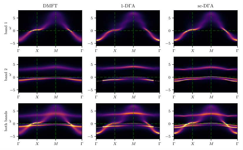
In the context of an orbital-selective Mott transition Anisimov et al. 2002; Liebsch 2003; Liebsch 2004; Koga et al. 2005; Biermann et al. 2005; Arita and Held 2005; Knecht et al. 2005; Sakai et al. 2006; Ferrero et al. 2005; Costi and Liebsch 2007; Koga et al. 2004; Greger et al. 2013; Valli et al. 2015b; Tocchio et al. 2016; Philipp et al. 2017; Hu et al. 2017, such simple half-filled two-band models with different bandwidths and intra-orbital hopping have been studied very intensively in DMFT. Early calculations however did not include the spin flip and pair hopping processes, but only the density-density interactions for technical reasons. In this situation, the tendency toward an orbital selective Mott transition is largely exaggerated: a spin formed by the Hund’s exchange cannot undergo a joint SU(4) Kondo effect, while the spin-1 of the SU(2)-symmetric interaction can. As we are primarily interested in testing the sc-DA method, we consider here the case where the model is doped away from half-filling or electrons per site. Specifically, we consider the doping . This gives rise also to a non-zero real part of the self-energy and (slightly) different fillings of the two orbitals; and hence tests various aspects at the same time.
In Fig. 14 we show the self-energy at selective -points. For the given parameters, the 1-DA corrections to the self-energy are extremely strong, even exceeding the value of the DMFT self-energy. The reason for this is that we are quite close to an (incommensurate) antiferromagnetic phase transition in DMFT. Immediately before the phase transition, the 1-DA corrections become even larger and turn the system insulating.
Similar as for the one-band model, the self-consistency suppresses the antiferromagnetic fluctuations; the actual phase transition occurs only at zero temperature because we are in two dimensions. Hence the sc-DA corrections are much weaker at the fixed temperature close to the DMFT phase transition. They will, as a matter of course, become stronger at lower temperatures which are not reachable by 1-DA exactly because of the DMFT phase transition. Indeed, Fig. 14 suggests that sc-DA is not too distinct from the DMFT result. That is, the self-consistency dampens away much of the one-shot corrections.
However, there is actually a quite important difference: Depending on the -point the sc-DA imaginary part of the self-energy at low Matsubara frequencies is above or below the DMFT self-energy in Fig. 14. This becomes even more obvious in Fig. 13, where we plot the self-energy at the lowest Matsubara frequency and see that the low frequency self-energy strongly depends on the momentum. A strong momentum differentiation of the imaginary part of the self-energy (i. e. the scattering rate) has also been reported for a SrVO3 monolayer Pickem et al. 2020.
In contrast to the imaginary part, the real part of the self-energy only shows a weak momentum dependence around the DMFT value in Fig. 13. This is different for 1-DA where the strong corrections are also reflected in a sizable momentum-dependence of the real part of the self-energy; the strongly correlated band (band 2; blue) also displays a sizable overall shift compared to the DMFT result in 1-DA.
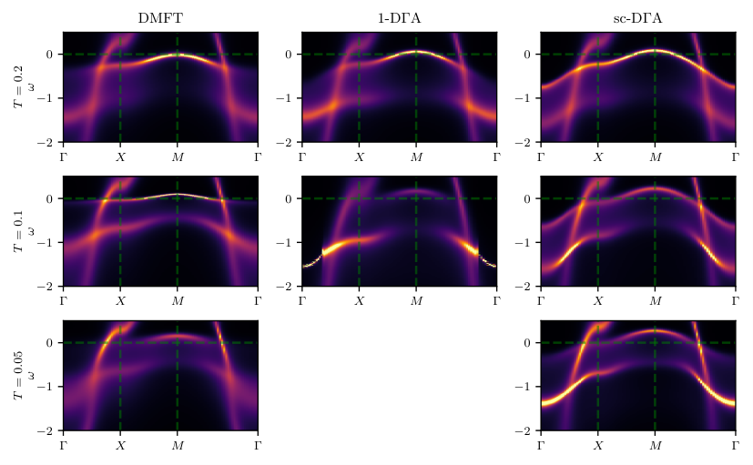
But let us turn back to the momentum dependence of the self-energy in sc-DA. It has a larger influence on the spectral function (Fig. 15) than what one might expect from the Matsubara-frequency dependence in Fig. 14. In Fig. 15 we see, for all three methods, that the weakly correlated band 1 is still close to the tight-binding starting point in Fig. 12, whereas the strongly correlated band 2 is split into an upper Hubbard band (around ), a lower Hubbard band (around ), and a central quasiparticle peak around the Fermi level (). The last is better visible in the zoom-in provided by Fig. 16. The aforementioned momentum differentiation of the self-energy results in a considerably wider central quasiparticle band in sc-DA than in DMFT or 1-DA. In 1-DA the strong fluctuations around the phase transition also smear out the central band when reducing temperature from to ; is below the DMFT ordering temperature and a one-shot calculation is hence no-longer possible (the reduction of the Néel temperature and susceptibility requires the self-consistency or a Moriya -correction Katanin et al. 2009).
In Fig. 17, we further show the spectral weight at the Fermi level in DMFT and sc-DA, summed over both orbitals. Clearly a Fermi surface close to the tight binding ones is visible. This stems mostly from the wide, less correlated band. The narrow, strongly correlated band is slightly shifted downwards to lower energy and considerably broadened, cf. Fig. 16. Since the band is so flat, this tiny shift results in a sizeable deformation of the spectral weight distribution on the Fermi level: Considering also that averages over a frequency range , we get diffuse arcs around the -point, i.e., , which is visible in Fig. 17. However, due to the strong renormalization that is already present in DMFT, the narrow band gives only a small contribution to the spectral weight on the Fermi level.


V.2 Strontium vanadate
As a second, archetypical multi-orbital application we study bulk strontium vanadate SrVO3 at room temperature (meV). This material has served as a testbed for the development of realistic materials calculations with strong correlations, and is hence most intensively studied Sekiyama et al. 2004; Pavarini et al. 2004; Nekrasov et al. 2006; Maiti et al. 2006; Leonov et al. 2014; Karolak et al. 2011; Lee et al. 2012; Casula et al. 2012; Tomczak et al. 2012; Taranto et al. 2013; Miyake et al. 2013; Sakuma et al. 2013; Tomczak et al. 2014; Wadati et al. 2014; Ribic et al. 2014; Zhong et al. 2015; Nakamura et al. 2016a; Boehnke et al. 2016; Nakamura et al. 2016b; Backes et al. 2016; Bhandary et al. 2016; J. M. Tomczak et al. 2017; Kaufmann et al. 2017; Bauernfeind et al. 2017; Sim and Han 2019. Also the first realistic materials calculations using diagrammatic extensions of DMFT, i.e., ab initio DA, have been performed for this perovskite Galler et al. 2017. SrVO3 is a strongly correlated metal with a quasiparticle renormalization of about two Sekiyama et al. 2004. Electronic correlations also lead to a kink in the self-energy and energy-momentum dispersion relation Nekrasov et al. 2006; Byczuk et al. 2007; Aizaki et al. 2012; Held et al. 2013. Theoretical calculations and experiments do not indicate any long-range order.
For this realistic ab initio calculation, we start with a Wien2K calculation Blaha et al. 2001; Schwarz et al. 2002 using the PBE exchange correlation potential in the generalized gradient approximation (GGA) Perdew et al. 1996, and a lattice constant of Å. The calculated bandstructure is projected onto maximally localized Wannier orbitals Pizzi et al. 2020; Marzari et al. 2012; Mostofi et al. 2008 using wien2wannier Kuneš et al. 2010 This three-band Wannier Hamiltonian, available open source 88 8 See https://github.com/AbinitioDGA/ADGA/blob/master/srvo3-testdata/srvo3_k20.hk, is supplemented by a Kanamori Coulomb interaction including the same terms as for the two-band model and parameterized by eV, eV and corresponding eV. The interactions and have been calculated by the constrained local density approximation (cLDA) in Sekiyama et al. 2004; was later slightly corrected as outlined in Section 4.1.3 of Held 2007 to account for the precise way enters in Hamiltonian (II.1) and the cLDA. The difference to earlier ab initio DA Galler et al. 2017; Galler et al. 2018; Galler et al. 2019 calculations, which have been one-shot non-self-consistent calculations, is that we now perform a self-consistent calculation.
As already mentioned, a Moriya- correction is extremely difficult for such realistic multi-orbital calculations. There is not only a magnetic and charge for every orbital but additionally also various orbital combinations. Hence, we hold that a self-consistent calculation shall be preferable compared to a high-dimensional fit of the various parameters. Also conceptionally it is a clearer approach.
In Fig. 18 we compare the self-energy of the one-shot and self-consistent DA calculation. In contrast to the two-band Hubbard model study above, the differences are here only minor. The reason for this is that in case of the two-band Hubbard model we were close to the DMFT phase transition, whereas SrVO3 is rather far away from any phase transition. Hence, the 1-DA corrections are much smaller to start with. In such a situation, the self-consistency is not necessary. This justifies a posteriori the use of non-self-consistent DA in Refs. Galler et al. 2017; Galler et al. 2018; Galler et al. 2019.
Nevertheless, Fig. 19 indicates some minor differences between the DMFT, 1-DA and sc-DA spectral functions. There are minor differences between 1-DA and sc-DA regarding the weight of the lower Hubbard band and the broadening of the quasiparticle peak. This behavior is perfectly in-line with the effect of 1-DA in other systems studied above. Furthermore there is a shift of the position of the lower Hubbard band toward lower binding energies visible at the point. Experimentally, the maximum of the lower Hubbard band is slightly above -2 eV Sekiyama et al. 2004.
VI Conclusion
We have presented a self-consistent solution of the ladder DA equations where the calculated DA self-energy is fed back into the Bethe-Salpeter ladder. This dampens the Green’s function and thus the overall strength of the ladder, largely reducing the critical temperatures of DMFT. Hitherto, a similar effect has been achieved by a Moriyaesque correction for one band-models; multi-orbital models have only been studied by one-shot, non-self-consistent and non--corrected calculations. Applying such a correction to multi-orbital or doped systems is difficult, to say the least. One-shot calculations, on the other hand, are disputable whenever the non-local corrections to DMFT become large. Our paper demonstrates that conceptionally clean self-consistent calculations are indeed feasible and work well, also for multi-orbital and doped systems.
For the one-band Hubbard model we have benchmarked the method against previous (-corrected and parquet) DA and numerically exact DiagMC results at weak coupling. We find an excellent agreement up to the point where the susceptibilities become huge, where self-consistent DA yields a somewhat reduced susceptibility. The self-consistency allows applying DA even in the close vicinity of the divergence lines of the vertex, at strong coupling and for doped systems.
For the two-band Hubbard model we study the regime close to the DMFT phase transition. Here, the one-shot DA corrections are large but the self-consistency mitigates this to a large extent. While the frequency dependence eventually looks similar to that of DMFT, there is a sizable momentum dependence which leads to a widening of the quasiparticle band. In case of SrVO3 we have performed realistic ab initio DA materials calculations. Here, we are not close to any phase transition and the difference between one-shot and self-consistent ab initio DA is minute.
Acknowledgements.
We thank Thomas Schäfer, Fedor Šimkovic and Patrick Chalupa for providing reference data; and Patrik Thunström, Anna Galler and Jan M. Tomczak for fruitful discussions and valuable advice. JK further thanks Oleg Janson, Alexander Lichtenstein, Andrey Katanin, Jan Kuneš, Evgeny Stepanov, Patrik Gunacker, Tin Ribic, Dominique Geffroy and Benedikt Hartl for fruitful discussions. This work has been supported financially by the European Research Council under the European Union’s Seventh Framework Program (FP/2007-2013)/ERC grant agreement n. 306447 and by the Austrian Science Fund (FWF) through projects P 30997, P 30819 and P 32044. Calculations have been done in part on the Vienna Scientific Cluster (VSC).Appendix A Implementation
For the practical evaluation of the DA equations Eqs. 21 to 23, we use the ab initio DA code Galler et al. 2019. Here we describe the details of the implementation, which are closely connected to ab initio DA. Solving the aforementioned equations self-consistently means that the ab initio DA code is executed several times in a loop in order to do a fixed-point iteration. Before each iteration, we create an updated trial input, until the point where the output does not differ from the input any more. Therefore, in order to describe the details of the updates, we have to recapitulate the input structure of ab initio DA first.
Apart from the system-defining parameters (tight-binding Hamiltonian and U-matrix) the following quantities are required as input:
- 1.
lattice self-energy (can also be momentum-independent)
- 2.
impurity self-energy (can be identical to the lattice self-energy, as in 1-DA)
- 3.
impurity Green’s function
- 4.
impurity two-particle Green’s function
The update proceeds in the two steps described in the following.
A.1 Update of the self-energy and one-particle Green’s function
This step defines the update. We take trial and result self-energies from several preceeding iterations and compose a new trial self-energy for the -th iteration. This is prediction is usually made by the Anderson acceleration algorithm Anderson 1965; Walker and Ni 2011 (also known as Pulay-mixing Pulay 1980 or direct inversion in iterative subspace, DIIS Császár and Pulay 1984). This trial self-energy is then used to compute a new local propagator by
| (25) |
where the chemical potential is adapted such that the expectation value of the particle number stays at the desired value. The change of the chemical potential usually stays in the range of a few percent. Once the new local Green’s function is determined, we project (downfold) it to the correlated impurity subspaces. Thus, each impurity obtains its new Green’s function .
A.2 Update of impurity quantities
This step is inherent to our specific implementation of ab initio DA, and not part of the algorithm per se. But since ab initio DA reads the one- and two-particle Green’s function instead of the irreducible vertex, we need to “wrap” the irreducible vertex (unchanged throughout all iterations) in the new impurity propagator by means of the Bethe-Salpeter equation. In order to avoid direct computation of the irreducible vertex, we compute the updated generalized susceptibility for iteration in channel by
| (26) |
Note that all susceptibilities in this equations are compound-index matrices in the orbital space of the impurity and fermionic frequencies. The new impurity one-particle Green’s function enters into this equation only through of Eq. 9, where updated impurity Green’s functions are used. The two-particle Green’s function is obtained by dividing through and adding a disconnected part, according to Eq. 7.
Furthermore, it is necessary to compute an updated (“fake”) impurity self-energy by the equation of motion. The reason for this can be seen in Eq. (75) of Ref. Galler et al. 2017. There, the DMFT self-energy appears as a separate term. However, in its essence it is not the DMFT self-energy, but rather the result of the Schwinger-Dyson equation of motion for the impurity99 9 We thank Patrik Thunström for drawing our attention to this crucial insight.. In Ref. Galler et al. 2017, this term is subtracted and substituted by the actual DMFT self-energy, in order to mitigate effects of finite frequency boxes. Therefore, we compute the impurity self-energy from the equation of motion,
| (27) |
using both the new and the DMFT one- and two-particle Green’s function. The index labels the -th impurity of the unit cell. Importantly, the frequency boxes have to be identical. Then the difference of these two self-energies is added to the DMFT self-energy and taken as the new (fake) impurity self-energy. In this way the effects of finite-box summation are cancelled. We emphasize that the “fake” impurity self-energy is merely an auxiliary quantity and never used to extract any physical properties of the result. Only the lattice self-energy is subject to physical interpretation in our computations.
Appendix B Extrapolation of the susceptibility
Since we are quite limited in the number of -points that we can use in our calculation, we have to do an extrapolation of the magnetic susceptibility. This is possible due to the observation that the inverse of the antiferromagnetic susceptibility depends linearly on the inverse of the number of -points. In particluar, the extrapolation was necessary for sc-DA on the square-lattice Hubbard model with at and . There the DA calculation was done with 4848, 6464, 6868, 7272, 7676, 8080 - and -points. In Fig. 20 and Fig. 21 it is visible that the extrapolation with above mentioned linear relation is indeed possible. Although a deviation from this behavior is to be expected as , it can only lead to a small change in the logarithmic plot in Fig. 4 and thus our conclusions remain unchanged.
On the other hand, for - and -grids of 4848 or larger, we find that the self-energy is practically independent on the number of - and -points, such that no extrapolation is necessary there.
References
- Hohenberg and Kohn (1964) P. Hohenberg and W. Kohn, Phys. Rev. 136, B864 (1964).
- Jones and Gunnarsson (1989) R. O. Jones and O. Gunnarsson, Rev. Mod. Phys. 61, 689 (1989).
- Metzner and Vollhardt (1989) W. Metzner and D. Vollhardt, Phys. Rev. Lett. 62, 324 (1989).
- Georges and Kotliar (1992) A. Georges and G. Kotliar, Phys. Rev. B 45, 6479 (1992).
- Jarrell (1992) M. Jarrell, Phys. Rev. Lett. 69, 168 (1992).
- Georges et al. (1996) A. Georges, G. Kotliar, W. Krauth, and M. J. Rozenberg, Rev. Mod. Phys. 68, 13 (1996).
- Kotliar and Vollhardt (2004) G. Kotliar and D. Vollhardt, Physics Today 57, 53 (2004).
- Anisimov et al. (1997) V. I. Anisimov, A. I. Poteryaev, M. A. Korotin, A. O. Anokhin, and G. Kotliar, Journal of Physics: Condensed Matter 9, 7359 (1997).
- Lichtenstein and Katsnelson (1998) A. I. Lichtenstein and M. I. Katsnelson, Phys. Rev. B 57, 6884 (1998).
- Held et al. (2006) K. Held, I. A. Nekrasov, G. Keller, V. Eyert, N. Blümer, A. K. McMahan, R. T. Scalettar, T. Pruschke, V. I. Anisimov, and D. Vollhardt, physica status solidi (b) 243, 2599 (2006).
- Kotliar et al. (2006) G. Kotliar, S. Y. Savrasov, K. Haule, V. S. Oudovenko, O. Parcollet, and C. A. Marianetti, Rev. Mod. Phys. 78, 865 (2006).
- Held (2007) K. Held, Advances in physics 56, 829 (2007).
- Gull et al. (2011) E. Gull, A. J. Millis, A. I. Lichtenstein, A. N. Rubtsov, M. Troyer, and P. Werner, Rev. Mod. Phys. 83, 349 (2011).
- Rohringer et al. (2018) G. Rohringer, H. Hafermann, A. Toschi, A. A. Katanin, A. E. Antipov, M. I. Katsnelson, A. I. Lichtenstein, A. N. Rubtsov, and K. Held, Rev. Mod. Phys. 90, 025003 (2018).
- Galler et al. (2017) A. Galler, P. Thunström, P. Gunacker, J. M. Tomczak, and K. Held, Phys. Rev. B 95, 115107 (2017).
- Galler et al. (2018) A. Galler, J. Kaufmann, P. Gunacker, M. Pickem, P. Thunström, J. M. Tomczak, and K. Held, Journal of the Physical Society of Japan 87, 041004 (2018).
- Galler et al. (2019) A. Galler, P. Thunström, J. Kaufmann, M. Pickem, J. M. Tomczak, and K. Held, Computer Physics Communications 245, 106847 (2019).
- Toschi et al. (2007a) A. Toschi, A. A. Katanin, and K. Held, Phys. Rev. B 75, 045118 (2007a).
- Katanin et al. (2009) A. A. Katanin, A. Toschi, and K. Held, Phys. Rev. B 80, 075104 (2009).
- Rohringer and Toschi (2016) G. Rohringer and A. Toschi, Phys. Rev. B 94, 125144 (2016).
- Rohringer et al. (2011) G. Rohringer, A. Toschi, A. Katanin, and K. Held, Phys. Rev. Lett. 107, 256402 (2011).
- Schäfer et al. (2017) T. Schäfer, A. A. Katanin, K. Held, and A. Toschi, Phys. Rev. Lett. 119, 046402 (2017).
- Schäfer et al. (2019) T. Schäfer, A. A. Katanin, M. Kitatani, A. Toschi, and K. Held, Phys. Rev. Lett. 122, 227201 (2019).
- Kitatani et al. (2019) M. Kitatani, T. Schäfer, H. Aoki, and K. Held, Phys. Rev. B 99, 041115 (2019).
- Kitatani et al. (2020) M. Kitatani, L. Si, O. Janson, R. Arita, Z. Zhong, and K. Held, npj Quantum Materials 5, 59 (2020).
- Rubtsov et al. (2008) A. N. Rubtsov, M. I. Katsnelson, and A. I. Lichtenstein, Phys. Rev. B 77, 033101 (2008).
- Hafermann et al. (2009) H. Hafermann, G. Li, A. N. Rubtsov, M. I. Katsnelson, A. I. Lichtenstein, and H. Monien, Phys. Rev. Lett. 102, 206401 (2009).
- Hirschmeier et al. (2015) D. Hirschmeier, H. Hafermann, E. Gull, A. I. Lichtenstein, and A. E. Antipov, Phys. Rev. B 92, 144409 (2015).
- Antipov et al. (2014) A. E. Antipov, E. Gull, and S. Kirchner, Phys. Rev. Lett. 112, 226401 (2014).
- Ribic et al. (2018) T. Ribic, P. Gunacker, and K. Held, Phys. Rev. B 98, 125106 (2018).
- van Loon et al. (2018) E. G. C. P. van Loon, M. I. Katsnelson, and H. Hafermann, Phys. Rev. B 98, 155117 (2018).
- Tanaka (2019) A. Tanaka, Phys. Rev. B 99, 205133 (2019).
- Valli et al. (2015a) A. Valli, T. Schäfer, P. Thunström, G. Rohringer, S. Andergassen, G. Sangiovanni, K. Held, and A. Toschi, Phys. Rev. B 91, 115115 (2015a).
- Li et al. (2016) G. Li, N. Wentzell, P. Pudleiner, P. Thunström, and K. Held, Phys. Rev. B 93, 165103 (2016).
- Li et al. (2019) G. Li, A. Kauch, P. Pudleiner, and K. Held, Computer Physics Communications 241, 146 (2019).
- Kauch et al. (2019) A. Kauch, F. Hörbinger, G. Li, and K. Held, arXiv e-prints , arXiv:1901.09743 (2019), arXiv:1901.09743 [cond-mat.str-el] .
- Eckhardt et al. (2020) C. J. Eckhardt, C. Honerkamp, K. Held, and A. Kauch, Phys. Rev. B 101, 155104 (2020).
- (38) For the parquet dual fermion approach, see Astleithner et al. 2020; Astretsov et al. 2020; Krien et al. 2020.
- De Dominicis and Martin (1964a) C. De Dominicis and P. C. Martin, Journal of Mathematical Physics 5, 14 (1964a), https://doi.org/10.1063/1.1704062 .
- De Dominicis and Martin (1964b) C. De Dominicis and P. C. Martin, Journal of Mathematical Physics 5, 31 (1964b), https://doi.org/10.1063/1.1704064 .
- Bickers (2004) N. E. Bickers, in Theoretical Methods for Strongly Correlated Electrons. CRM Series in Mathematical Physics, edited by D. Sénéchal, A.-M. Tremblay, and C. Bourbonnais (Springer, 2004).
- Vasil’ev (1998) A. N. Vasil’ev, Functional Methods in Quantum Field Theory and Statistical Physics, 1st ed., 1, Vol. 1 (Taylor and Francis Group, 1998).
- Kauch et al. (2020) A. Kauch, P. Pudleiner, K. Astleithner, P. Thunström, T. Ribic, and K. Held, Phys. Rev. Lett. 124, 047401 (2020).
- Rohringer et al. (2012) G. Rohringer, A. Valli, and A. Toschi, Phys. Rev. B 86, 125114 (2012).
- Gunacker et al. (2015) P. Gunacker, M. Wallerberger, E. Gull, A. Hausoel, G. Sangiovanni, and K. Held, Phys. Rev. B 92, 155102 (2015).
- Wallerberger et al. (2019) M. Wallerberger et al., Computer Physics Communications 235, 388 (2019).
- (47) And often dangerous!
- Toschi et al. (2007b) A. Toschi, A. A. Katanin, and K. Held, Phys. Rev. B 75, 045118 (2007b).
- Schäfer et al. (2016) T. Schäfer, A. Toschi, and K. Held, Journal of Magnetism and Magnetic Materials 400, 107 (2016), proceedings of the 20th International Conference on Magnetism (Barcelona) 5-10 July 2015.
- Kugler and von Delft (2018) F. B. Kugler and J. von Delft, New Journal of Physics 20, 123029 (2018).
- Hille et al. (2020) C. Hille, F. B. Kugler, C. J. Eckhardt, Y.-Y. He, A. Kauch, C. Honerkamp, A. Toschi, and S. Andergassen, Phys. Rev. Research 2, 033372 (2020).
- Metzner et al. (2012) W. Metzner, M. Salmhofer, C. Honerkamp, V. Meden, and K. Schönhammer, Rev. Mod. Phys. 84, 299 (2012).
- (53) That is, cutting any two Green’s function lines does not separate the Feynman diagram into two pieces.
- (54) It is not necessary to take from DMFT. One could improve the auxiliary Anderson impurity model, so that it produced the same local Green’s function as the one resulting from p-DA. It would add another level of self-consistency. This impurity update turned out to be unnecessary for the parameters presented in this paper.
- Husemann and Salmhofer (2009) C. Husemann and M. Salmhofer, Phys. Rev. B 79, 195125 (2009).
- Eckhardt et al. (2018) C. J. Eckhardt, G. A. H. Schober, J. Ehrlich, and C. Honerkamp, Phys. Rev. B 98, 075143 (2018).
- Schäfer et al. (2013) T. Schäfer, G. Rohringer, O. Gunnarsson, S. Ciuchi, G. Sangiovanni, and A. Toschi, Phys. Rev. Lett. 110, 246405 (2013).
- Schäfer et al. (2016) T. Schäfer, S. Ciuchi, M. Wallerberger, P. Thunström, O. Gunnarsson, G. Sangiovanni, G. Rohringer, and A. Toschi, Phys. Rev. B 94, 235108 (2016).
- Gunnarsson et al. (2017) O. Gunnarsson, G. Rohringer, T. Schäfer, G. Sangiovanni, and A. Toschi, Phys. Rev. Lett. 119, 056402 (2017).
- Vučičević et al. (2018) J. Vučičević, N. Wentzell, M. Ferrero, and O. Parcollet, Phys. Rev. B 97, 125141 (2018).
- Chalupa et al. (2018) P. Chalupa, P. Gunacker, T. Schäfer, K. Held, and A. Toschi, Phys. Rev. B 97, 245136 (2018).
- (62) In some cases it may be preferable to take the non-local particle-particle fluctuations as dominant and approximate the particle-hole channel to the local level. In the scope of this paper we treat however only problems with dominant fluctuations in the particle-hole channel.
- Mermin and Wagner (1966) N. D. Mermin and H. Wagner, Phys. Rev. Lett. 17, 1307 (1966).
- Schäfer et al. (2020) T. Schäfer, N. Wentzell, F. Šimkovic IV, Y.-Y. He, C. Hille, M. Klett, C. J. Eckhardt, B. Arzhang, V. Harkov, F.-M. L. Régent, A. Kirsch, Y. Wang, A. J. Kim, E. Kozik, E. A. Stepanov, A. Kauch, S. Andergassen, P. Hansmann, D. Rohe, Y. M. Vilk, J. P. F. LeBlanc, S. Zhang, A. M. S. Tremblay, M. Ferrero, O. Parcollet, and A. Georges, Tracking the footprints of spin fluctuations: A multi-method, multi-messenger study of the two-dimensional hubbard model (2020), arXiv:2006.10769 [cond-mat.str-el] .
- Miyahara et al. (2013) H. Miyahara, R. Arita, and H. Ikeda, Phys. Rev. B 87, 045113 (2013).
- Arya et al. (2015) S. Arya, P. V. Sriluckshmy, S. R. Hassan, and A.-M. S. Tremblay, Phys. Rev. B 92, 045111 (2015).
- Tremblay (2011) A. M. S. Tremblay, in Strongly Correlated Systems: Theoretical Methods, edited by F. Mancini and A. Avella (Springer, Berlin, Heidelberg, 2011) Chap. 13, p. 409–455.
- Anderson (1965) D. G. Anderson, J. ACM 12, 547–560 (1965).
- Walker and Ni (2011) H. F. Walker and P. Ni, SIAM Journal on Numerical Analysis 49, 1715 (2011), https://doi.org/10.1137/10078356X .
- Ayral and Parcollet (2016) T. Ayral and O. Parcollet, Phys. Rev. B 94, 075159 (2016).
- (71) Actually, for Kanamori interaction we find where are octagonal numbers.
- Kaufmann et al. (2019) J. Kaufmann, P. Gunacker, A. Kowalski, G. Sangiovanni, and K. Held, Phys. Rev. B 100, 075119 (2019).
- Kappl et al. (2020) P. Kappl, M. Wallerberger, J. Kaufmann, M. Pickem, and K. Held, Phys. Rev. B 102, 085124 (2020).
- Kuneš (2011) J. Kuneš, Phys. Rev. B 83, 085102 (2011).
- Geffroy et al. (2019) D. Geffroy, J. Kaufmann, A. Hariki, P. Gunacker, A. Hausoel, and J. Kuneš, Phys. Rev. Lett. 122, 127601 (2019).
- Kaufmann (2020) J. Kaufmann, ana_cont: Package for analytic continuation of many-body green’s functions, https://github.com/josefkaufmann/ana_cont (2020).
- Y.M. Vilk and A.-M.S. Tremblay (1997) Y.M. Vilk and A.-M.S. Tremblay, J. Phys. I France 7, 1309 (1997).
- Rubtsov et al. (2009) A. N. Rubtsov, M. I. Katsnelson, A. I. Lichtenstein, and A. Georges, Phys. Rev. B 79, 045133 (2009).
- Rost et al. (2012) D. Rost, E. V. Gorelik, F. Assaad, and N. Blümer, Phys. Rev. B 86, 155109 (2012).
- Schäfer et al. (2015) T. Schäfer, F. Geles, D. Rost, G. Rohringer, E. Arrigoni, K. Held, N. Blümer, M. Aichhorn, and A. Toschi, Phys. Rev. B 91, 125109 (2015).
- González et al. (2000) J. González, F. Guinea, and M. A. H. Vozmediano, Phys. Rev. Lett. 84, 4930 (2000).
- Halboth and Metzner (2000) C. J. Halboth and W. Metzner, Phys. Rev. Lett. 85, 5162 (2000).
- Honerkamp and Salmhofer (2001) C. Honerkamp and M. Salmhofer, Phys. Rev. Lett. 87, 187004 (2001).
- Wu et al. (2020) W. Wu, M. S. Scheurer, M. Ferrero, and A. Georges, Phys. Rev. Research 2, 033067 (2020).
- Šimkovic and Kozik (2019) F. Šimkovic and E. Kozik, Phys. Rev. B 100, 121102 (2019).
- (86) In this case the Ward identity relating the irreducible vertex and self-energy is violated. This is also the case in the parquet approach, but certainly to a much smaller extent.
- Gull et al. (2013) E. Gull, O. Parcollet, and A. J. Millis, Phys. Rev. Lett. 110, 216405 (2013).
- Chen et al. (2013) K.-S. Chen, Z. Y. Meng, S.-X. Yang, T. Pruschke, J. Moreno, and M. Jarrell, Phys. Rev. B 88, 245110 (2013).
- Otsuki et al. (2014) J. Otsuki, H. Hafermann, and A. I. Lichtenstein, Phys. Rev. B 90, 235132 (2014).
- Jia et al. (2014) C. J. Jia, E. A. Nowadnick, K. Wohlfeld, Y. F. Kung, C.-C. Chen, S. Johnston, T. Tohyama, B. Moritz, and T. P. Devereaux, Nature Communications 5, 3314 (2014).
- LeBlanc et al. (2019) J. P. F. LeBlanc, S. Li, X. Chen, R. Levy, A. E. Antipov, A. J. Millis, and E. Gull, Phys. Rev. B 100, 075123 (2019).
- Chan et al. (2016) M. K. Chan, C. J. Dorow, L. Mangin-Thro, Y. Tang, Y. Ge, M. J. Veit, G. Yu, X. Zhao, A. D. Christianson, J. T. Park, Y. Sidis, P. Steffens, D. L. Abernathy, P. Bourges, and M. Greven, Nature Communications 7, 10819 (2016).
- Anisimov et al. (2002) V. Anisimov, I. Nekrasov, D. Kondakov, T. Rice, and M. Sigrist, Eur. Phys. J. B 25, 97 (2002).
- Liebsch (2003) A. Liebsch, Europhysics Letters (EPL) 63, 97 (2003).
- Liebsch (2004) A. Liebsch, Phys. Rev. B 70, 165103 (2004).
- Koga et al. (2005) A. Koga, N. Kawakami, T. M. Rice, and M. Sigrist, Phys. Rev. B 72, 045128 (2005).
- Biermann et al. (2005) S. Biermann, L. de’ Medici, and A. Georges, Phys. Rev. Lett. 95, 206401 (2005).
- Arita and Held (2005) R. Arita and K. Held, Phys. Rev. B 72, 201102 (2005).
- Knecht et al. (2005) C. Knecht, N. Blümer, and P. G. J. van Dongen, Phys. Rev. B 72, 081103 (2005).
- Sakai et al. (2006) S. Sakai, R. Arita, K. Held, and H. Aoki, Phys. Rev. B 74, 155102 (2006).
- Ferrero et al. (2005) M. Ferrero, F. Becca, M. Fabrizio, and M. Capone, Phys. Rev. B 72, 205126 (2005).
- Costi and Liebsch (2007) T. A. Costi and A. Liebsch, Phys. Rev. Lett. 99, 236404 (2007).
- Koga et al. (2004) A. Koga, N. Kawakami, T. M. Rice, and M. Sigrist, Phys. Rev. Lett. 92, 216402 (2004).
- Greger et al. (2013) M. Greger, M. Kollar, and D. Vollhardt, Phys. Rev. Lett. 110, 046403 (2013).
- Valli et al. (2015b) A. Valli, H. Das, G. Sangiovanni, T. Saha-Dasgupta, and K. Held, Phys. Rev. B 92, 115143 (2015b).
- Tocchio et al. (2016) L. F. Tocchio, F. Arrigoni, S. Sorella, and F. Becca, J. Phys.: Condensed Matter 28, 105602 (2016).
- Philipp et al. (2017) M.-T. Philipp, M. Wallerbegrr, P. Gunacker, and K. Held, Eur. Phys. J. B 0, 114 (2017).
- Hu et al. (2017) W. Hu, R. T. Scalettar, E. W. Huang, and B. Moritz, Phys. Rev. B 95, 235122 (2017).
- Pickem et al. (2020) M. Pickem, J. Kaufmann, J. M. Tomczak, and K. Held, Particle-hole asymmetric lifetimes promoted by spin and orbital fluctuations in ultrahin srvo3 films (2020), arXiv:2008.12227 [cond-mat.str-el] .
- Sekiyama et al. (2004) A. Sekiyama, H. Fujiwara, S. Imada, S. Suga, H. Eisaki, S. I. Uchida, K. Takegahara, H. Harima, Y. Saitoh, I. A. Nekrasov, G. Keller, D. E. Kondakov, A. V. Kozhevnikov, T. Pruschke, K. Held, D. Vollhardt, and V. I. Anisimov, Phys. Rev. Lett. 93, 156402 (2004).
- Pavarini et al. (2004) E. Pavarini, S. Biermann, A. Poteryaev, A. I. Lichtenstein, A. Georges, and O. K. Andersen, Phys. Rev. Lett. 92, 176403 (2004).
- Nekrasov et al. (2006) I. A. Nekrasov, K. Held, G. Keller, D. E. Kondakov, T. Pruschke, M. Kollar, O. K. Andersen, V. I. Anisimov, and D. Vollhardt, Phys. Rev. B 73, 155112 (2006).
- Maiti et al. (2006) K. Maiti, U. Manju, S. Ray, P. Mahadevan, I. H. Inoue, C. Carbone, and D. D. Sarma, Phys. Rev. B 73, 052508 (2006).
- Leonov et al. (2014) I. Leonov, V. I. Anisimov, and D. Vollhardt, Phys. Rev. Lett. 112, 146401 (2014).
- Karolak et al. (2011) M. Karolak, T. O. Wehling, F. Lechermann, and A. I. Lichtenstein, J. Phys. Condens. Matter 23, 085601 (2011).
- Lee et al. (2012) H. Lee, K. Foyevtsova, J. Ferber, M. Aichhorn, H. O. Jeschke, and R. Valent\́mathrm{i}, Phys. Rev. B 85, 165103 (2012).
- Casula et al. (2012) M. Casula, A. Rubtsov, and S. Biermann, Phys. Rev. B 85, 035115 (2012).
- Tomczak et al. (2012) J. M. Tomczak, M. Casula, T. Miyake, F. Aryasetiawan, and S. Biermann, EPL (Europhysics Letters) 100, 67001 (2012).
- Taranto et al. (2013) C. Taranto, M. Kaltak, N. Parragh, G. Sangiovanni, G. Kresse, A. Toschi, and K. Held, Phys. Rev. B 88, 165119 (2013).
- Miyake et al. (2013) T. Miyake, C. Martins, R. Sakuma, and F. Aryasetiawan, Phys. Rev. B 87, 115110 (2013).
- Sakuma et al. (2013) R. Sakuma, P. Werner, and F. Aryasetiawan, Phys. Rev. B 88, 235110 (2013).
- Tomczak et al. (2014) J. M. Tomczak, M. Casula, T. Miyake, and S. Biermann, Phys. Rev. B 90, 165138 (2014).
- Wadati et al. (2014) H. Wadati, J. Mravlje, K. Yoshimatsu, H. Kumigashira, M. Oshima, T. Sugiyama, E. Ikenaga, A. Fujimori, A. Georges, A. Radetinac, K. S. Takahashi, M. Kawasaki, and Y. Tokura, Phys. Rev. B 90, 205131 (2014).
- Ribic et al. (2014) T. Ribic, E. Assmann, A. Tóth, and K. Held, Phys. Rev. B 90, 165105 (2014).
- Zhong et al. (2015) Z. Zhong, M. Wallerberger, J. M. Tomczak, C. Taranto, N. Parragh, A. Toschi, G. Sangiovanni, and K. Held, Phys. Rev. Lett. 114, 246401 (2015).
- Nakamura et al. (2016a) K. Nakamura, Y. Nohara, Y. Yosimoto, and Y. Nomura, Phys. Rev. B 93, 085124 (2016a).
- Boehnke et al. (2016) L. Boehnke, F. Nilsson, F. Aryasetiawan, and P. Werner, Phys. Rev. B 94, 201106 (2016).
- Nakamura et al. (2016b) K. Nakamura, Y. Nohara, Y. Yosimoto, and Y. Nomura, Phys. Rev. B 93, 085124 (2016b).
- Backes et al. (2016) S. Backes, T. C. Rödel, F. Fortuna, E. Frantzeskakis, P. Le Fèvre, F. Bertran, M. Kobayashi, R. Yukawa, T. Mitsuhashi, M. Kitamura, K. Horiba, H. Kumigashira, R. Saint-Martin, A. Fouchet, B. Berini, Y. Dumont, A. J. Kim, F. Lechermann, H. O. Jeschke, M. J. Rozenberg, R. Valent\́mathrm{i}, and A. F. Santander-Syro, Phys. Rev. B 94, 241110 (2016).
- Bhandary et al. (2016) S. Bhandary, E. Assmann, M. Aichhorn, and K. Held, Phys. Rev. B 94, 155131 (2016).
- J. M. Tomczak et al. (2017) J. J. M. Tomczak, P. Liu, A. Toschi, G. Kresse, and K. Held, Eur. Phys. J.: Special Topics 226, 2565 (2017).
- Kaufmann et al. (2017) J. Kaufmann, P. Gunacker, and K. Held, Phys. Rev. B 96, 035114 (2017).
- Bauernfeind et al. (2017) D. Bauernfeind, M. Zingl, R. Triebl, M. Aichhorn, and H. G. Evertz, Phys. Rev. X 7, 031013 (2017).
- Sim and Han (2019) J.-H. Sim and M. J. Han, Phys. Rev. B 100, 115151 (2019).
- Byczuk et al. (2007) K. Byczuk, M. Kollar, K. Held, Y.-F. Yang, I. A. Nekrasov, T. Pruschke, and D. Vollhardt, Nature Physics , 168 (2007).
- Aizaki et al. (2012) S. Aizaki, T. Yoshida, K. Yoshimatsu, M. Takizawa, M. Minohara, S. Ideta, A. Fujimori, K. Gupta, P. Mahadevan, K. Horiba, H. Kumigashira, and M. Oshima, Phys. Rev. Lett. 109, 056401 (2012).
- Held et al. (2013) K. Held, R. Peters, and A. Toschi, Phys. Rev. Lett. 110, 246402 (2013).
- Blaha et al. (2001) P. Blaha et al., An augmented plane wave + local orbitals program for calculating crystal properties (Technische Universitat Wien Vienna, 2001).
- Schwarz et al. (2002) K. Schwarz, P. Blaha, and G. Madsen, Comp. Phys. Commun. 147, 71 (2002).
- Perdew et al. (1996) J. P. Perdew, K. Burke, and M. Ernzerhof, Phys. Rev. Lett. 77, 3865 (1996).
- Pizzi et al. (2020) G. Pizzi et al., Journal of Physics: Condensed Matter 32, 165902 (2020).
- Marzari et al. (2012) N. Marzari, A. A. Mostofi, J. R. Yates, I. Souza, and D. Vanderbilt, Rev. Mod. Phys. 84, 1419 (2012).
- Mostofi et al. (2008) A. A. Mostofi, J. R. Yates, Y.-S. Lee, I. Souza, D. Vanderbilt, and N. Marzari, Computer physics communications 178, 685 (2008).
- Kuneš et al. (2010) J. Kuneš et al., Computer Physics Communications 181, 1888 (2010).
- (145) See https://github.com/AbinitioDGA/ADGA/blob/master/srvo3-testdata/srvo3_k20.hk.
- Pulay (1980) P. Pulay, Chemical Physics Letters 73, 393 (1980).
- Császár and Pulay (1984) P. Császár and P. Pulay, Journal of Molecular Structure 114, 31 (1984).
- (148) We thank Patrik Thunström for drawing our attention to this crucial insight.
- Astleithner et al. (2020) K. Astleithner, A. Kauch, T. Ribic, and K. Held, Phys. Rev. B 101, 165101 (2020).
- Astretsov et al. (2020) G. V. Astretsov, G. Rohringer, and A. N. Rubtsov, Phys. Rev. B 101, 075109 (2020).
- Krien et al. (2020) F. Krien, A. Valli, P. Chalupa, M. Capone, A. I. Lichtenstein, and A. Toschi, Phys. Rev. B 102, 195131 (2020).