Efficient Sampling from Feasible Sets of SDPs and Volume ApproximationJournal: …

Apostolos Chalkis Address: ATHENA Research Center, Greece Address: Department of Informatics & Telecommunications
National & Kapodistrian University of Athens, Greece Ioannis Z. Emiris Address: ATHENA Research Center, Greece Address: Department of Informatics & Telecommunications
National & Kapodistrian University of Athens, Greece Vissarion Fisikopoulos Address: Department of Informatics & Telecommunications
National & Kapodistrian University of Athens, Greece Panagiotis Repouskos Address: Department of Informatics & Telecommunications
National & Kapodistrian University of Athens, Greece Elias Tsigaridas Address: Inria Paris, IMJ-PRG,
Sorbonne Université and Paris Université

Abstract

We present algorithmic, complexity, and implementation results on the problem of sampling points from a spectrahedron, that is the feasible region of a semidefinite program.

Our main tool is geometric random walks. We analyze the arithmetic and bit complexity of certain primitive geometric operations that are based on the algebraic properties of spectrahedra and the polynomial eigenvalue problem. This study leads to the implementation of a broad collection of random walks for sampling from spectrahedra that experimentally show faster mixing times than methods currently employed either in theoretical studies or in applications, including the popular family of Hit-and-Run walks. The different random walks offer a variety of advantages, thus allowing us to efficiently sample from general probability distributions, for example the family of log-concave distributions which arise in numerous applications. We focus on two major applications of independent interest: (i) approximate the volume of a spectrahedron, and (ii) compute the expectation of functions coming from robust optimal control.

We exploit efficient linear algebra algorithms and implementations to address the aforementioned computations in very high dimension. In particular, we provide a C++ open source implementation of our methods that scales efficiently, for the first time, up to dimension 200. We illustrate its efficiency on various data sets.

Keywords:

spectahedra , semidefinite-programming , sampling , random walk , polynomial eigenvalue problem , volume approximation , optimization

1 Introduction

Spectrahedra are probably the most well studied shapes after polyhedra. We can represent polyhedra as the intersection of the positive orthant with an affine subspace. Spectrahedra generalize polyhedra, in the sense that they are the intersection of the cone of positive semidefinite matrices —i.e., symmetric matrices with non-negative eigenvalues— with an affine space. In other words, a spectrahedron $S\subset\mathbb{R}^{n}$ is the feasible set of a linear matrix inequality. That is, let

\bm{F}(\bm{x})=\bm{A}_{0}+x_{1}\bm{A}_{1}+\cdots+x_{n}\bm{A}_{n},

(1)

where $\bm{A}_{i}$ are symmetric matrices in $\mathbb{R}^{m\times m}$ , then $S=\{\bm{x}\in\mathbb{R}^{n}\,|\,\bm{F}(\bm{x})\succeq 0\}$ , where $\succeq$ denotes positive semidefiniteness. We assume throughout that $S$ is bounded of dimension $n$ . Spectrahedra are convex sets (Figures 2 and 4) and every polytope is a spectrahedron, but not the opposite. They are the feasible regions of semidefinite programs [47] in the way that polyhedra are feasible regions of linear programs.

Refer to caption — Figure 1: Left, a 3D elliptope (image from https://en.wikipedia.org/wiki/Spectrahedron); an elliptope –a special case of spectrahedron– is the set of all real, square symmetric matrices whose diagonal entries are all equal to one and whose eigenvalues are all non-negative. Right, a spectrahedron from [8]; it is called cubic spectrahedron.

Efficient methods for sampling points in spectrahedra are crucial for many applications, such as volume approximation [16], integration [39], semidefinite optimization [39, 27], and applications in robust control analysis [11, 10, 53]. To sample in the interior or on the boundary of $S$ , we employ geometric random walks [56]. A geometric random walk on $S$ starts at some interior point and at each step moves to a "neighboring" point that we choose according to some distribution, depending only on the current point; thus it is a special category of Markov chains. For example, in the so-called ball walk, we move to a point $p$ that we choose uniformly at random in a ball of fixed radius $\delta$ , if $p\in S$ . The complexity of a random walk depends on its mixing time —the number of steps required to bound the distance between the current and the stationary distribution— and the complexity of the basic geometric operations performed at each step of the walk; we call the latter per-step complexity.

The majority of geometric random walks are defined for general convex bodies and are based on an oracle; usually the membership oracle. There are also a few walks, e.g., Vaidya walk [14] and the sub-linear ball walk [41], specialized for polytopes. Most results on their analysis focus on convergence and mixing time, while they define abstractly the operations they perform at each step and they enclose them in the corresponding oracle. That is why the complexity bounds involve the number of oracle calls.

To specialize a random walk for a family or representation of convex bodies one has to come up with efficient algorithms for the basic geometric operations to realize the (various) oracles. These operations should exploit the underlying geometric and algebraic properties and are of independent interest. They depend on efficient (numerical) linear algebra computations. More importantly, they dominate the per-step complexity and are hence crucial both for the overall complexity to sample a point from the target distribution, as well as for an efficient implementation.

The study of basic geometric operations to sample from non-linear convex objects finds its roots in non-linear computational geometry. During the last two decades, there are combined efforts [7, 22] to develop efficient algorithms for the basic operations (predicates) that are behind classical geometric algorithms, like convex hull, arrangements, Voronoi diagrams, to go beyond points and lines and handle curved objects. For this, one exploits efficiently structure and symmetry in linear algebra computations, and develops novel algebraic tools.

To our knowledge, only the Random Directions Hit and Run (W-HnR) random walk [50] has been studied for spectrahedra [10]. To exploit the various other walks, like Ball walk [56], Billiard walk (W-Billard) [24], and Hamiltonian Monte Carlo with boundary reflections (W-HMC-r) [1], one needs to provide geometric operations. For example, we need to compute the reflection of a curve at the boundary, and the intersection point of a curve with the boundary (of a spectrahedron).

We should mention that there is a gap [17, 5] between the theoretical worst case bounds for the mixing times and the practical performance of the random walk algorithms. Furthermore, there are random walks without known theoretical mixing times, such as Coordinate Directions Hit and Run (W-CHnR), W-Billard and W-HMC-r. To study them experimentally, it is imperative to provide an efficient realization of the corresponding oracles.

Previous Work

Sampling convex sets via random walks has attracted a lot of interest in the last decades. Most of the works assume that the convex sets are polytopes; [41] provides an overview of the state-of-the-art. Random walks on spectrahedra are studied in [46, 18], where they exploit the W-HnR and the computation of the intersection of the walk with the boundary reduces to a generalized eigenvalue problem.

The W-Billard [24] is a general way of sampling in convex or non-convex shapes from the uniform distribution. A mathematical billiard consists of a domain $\mathcal{D}$ and a point-mass, moving freely in $\mathcal{D}$ [52]. When this point-mass hits the boundary, it performs a specular reflection, albeit without losing velocity. An application of billiards is the study of optical properties of conics [52, Section 4].

If the trajectory is not a line, but rather a parametric curve, then the intersection operation reduces to solving a polynomial eigenvalue problem (PEP); W-HMC-r requires this operation. PEP is a well-studied problem in computational mathematics, e.g., [54], and it appears in many applications. There are important results both for the perturbation analysis of PEP [54, 4, 19], as well as for the condition-based analysis of algorithms for the real and complex versions of PEP, if we assume random inputs [2, 3].

For the closely related problem of volume computation, there is also an extensive bibliography [9]. The bulk of the theoretical studies are either for general convex bodies [20, 16] or polytopes [35]. Practical algorithms and implementations exist only for polytopes [21, 17]. Nevertheless, there are notable exceptions that consider algorithms for computing the volume of compact (basic) semi-algebraic sets. For example, in [31] they exploit the periods of rational integrals. In the same setting, [30, 26] introduce numerical approximation schemes for volume computations, which rely on the moment-based algorithms and semi-definite programming.

Finally, sampling from a multivariate distribution is a central problem in numerous applications. For example, it is useful in robust control analysis [10, 11, 53] to overcome the worst case hardness as well as in integration [39] and convex optimization [18, 27].

Our contribution

We present a framework of basic geometric operations for computations with spectrahedra. In particular, we analyze the arithmetic and bit complexity of the three fundamental operations, membership, intersection, reflection, by reducing them to linear algebra computations. Based on this framework, we support a rich class of geometric random walks, which in turn we employ in order to build efficient methods for sampling points from spectahedra, under various probability distributions. We apply these tools to approximate the volume of spectrahedra, as well as to integrate over spectrahedral domains. This extends the limits of the state-of-the-art methods that sample from spectrahedra, which actually involve only the W-HnR [18, 10]. We offer an efficient C++ implementation of our algorithms as a development branch of the package volesti¹¹ 1 https://github.com/GeomScale/volume_approximation/tree/sample_spectrahedra, an open source library for high dimensional sampling and volume computation. While the implementation is in C++, there is also an R interface, for easier access to its functionality. Our implementation is based on state-of-the-art algorithms in numerical linear algebra to address computation in high dimension. Our software makes use of powerful C++ libraries such as Eigen [25] and Spectra [51].

We demonstrate the efficiency of our approach and implementation on problems from robust control and optimization. First, as a special case of integration, we approximate the volume of spectrahedra up to dimension 100; this is, to the best of our knowledge, the first time such computations for non-linear objects are performed in high dimensions. Then, we approximate the expected value of a function $f:\mathbb{R}^{n}\rightarrow[0,1]$ , whose argument is a random variable having uniform distribution over a spectrahedron of dimension $200$ .

Finally, we sample from the Boltzmann distribution using W-HMC-r; this exploits a random walk in a spectrahedron that employs a polynomial trajectory of degree two. Sampling using W-HMC-r from truncated distributions is a classical problem in computational statistics [15, 1]; alas, existing approaches handle either special distributions or special cases of constraints [42, 32]. We equip W-HMC-r with geometric operations to handle log-concave densities truncated by linear matrix inequalities (LMI) constraints. A combination of Boltzmann distribution with a simulated annealing technique [27] could lead to a practical solver for semidefinite programs (SDP).

A very short version of this paper has appeared as a poster in [13].

Paper organization

First, we introduce our notation. In Section 2 we introduce the basic geometric operations used to efficiently implement membership and boundary oracles. In Section 3, we develop the different types of random walks. Finally, Section 4 presents our implementation, our applications, and various experiments.

Notation

We denote by $\mathcal{O}$ , respectively $\mathcal{O}_{B}$ , the arithmetic, respectively bit, complexity and we use $\widetilde{\mathcal{O}}$ , respectively $\widetilde{\mathcal{O}}_{B}$ , to ignore (poly-)logarithmic factors. The bitsize of a univariate polynomial $A\in\mathbb{Z}[x]$ is the maximum bitsize of its coefficients. We use bold letters for matrices, $\bm{A}$ , and vectors, $\bm{v}$ ; we denote by $A_{i,j}$ , respectively $v_{i}$ , their elements; $\bm{A}^{\top}$ is the transpose and $\bm{A}^{*}$ the adjoint of $\bm{A}$ . If $\bm{x}=(x_{1},\dots,x_{n})$ , then $\bm{F}(\bm{x})=\bm{A}_{0}+\sum_{i=1}^{n}x_{i}\bm{A}_{i}$ , see (1). For two points $\bm{x}$ and $\bm{y}$ , we denote the line through them by $\ell(\bm{x},\bm{y})$ and their segment as $[\bm{x},\bm{y}]$ . For a spectrahedron $S$ , let its interior be $S^{\circ}$ and its boundary ${\partial S}$ . We represent a probability distribution $\pi$ with a probability density function $\pi(x)$ . When $\pi$ is truncated to $S$ the support of $\pi(x)$ is $S$ . If $\pi$ is log-concave, then $\pi(\bm{x})\propto e^{-\alpha f(\bm{x})}$ , where $f:\mathbb{R}^{d}\rightarrow\mathbb{R}$ a convex function. Finally, let $\mathcal{B}_{n}$ be the $n$ -dimensional unit ball and denote by ${\partial\mathcal{B}_{n}}$ its boundary.

2 Basic geometric operations

Our toolbox for computations with spectrahedra and implementing random walks, consists of three basic geometric operations: membership, intersection, and reflection.

For a spectrahedron $S$ , membership decides whether a point lies inside $S$ , intersection computes the intersection of an algebraic curved trajectory $\mathcal{C}$ with the boundary ${\partial S}$ , and reflection computes the reflection of an algebraic curved trajectory when it hits ${\partial S}$ . The last two operations are required because random walks can move along non-linear trajectories inside convex bodies. For those studied in this paper, the trajectories are parametric polynomial curves, of various degrees. Computation with these curves reduces to solving the polynomial eigenvalue problem (PEP).

2.1 Analysis of PEP

To estimate the complexity of intersection we need to bound the complexity of PEP. The Polynomial Eigenvalue Problem (PEP) consists in computing $\lambda\in\mathbb{R}$ and $\bm{x}\in\mathbb{R}^{m}$ that satisfy the (matrix) equation

P(\lambda)\,\bm{x}=0\Leftrightarrow(\bm{B}_{d}\lambda^{d}+\cdots+\bm{B}_{1}\lambda+\bm{B}_{0})\bm{x}=0\kern 5.0pt,

(2)

where $P(\lambda)$ is a univariate matrix polynomial whose coefficients are matrices $\bm{B}_{i}\in\mathbb{R}^{m\times m}$ . We further assume that $\bm{B}_{d}$ and $\bm{B}_{0}$ are invertible. In general, there are $\delta=m\,d$ values of $\lambda$ . We refer the reader to [54] for a thorough exposition of PEP.

One approach for solving PEP is to linearalize the problem and to express the $\lambda$ ’s as the eigenvalues of a larger matrix. For this, we transform Equation (2) into a linear pencil of dimension $\delta$ . Following [4], the Companion Linearization consists in solving the generalized eigenvalue problem $\bm{C}_{0}-\lambda\bm{C}_{1}$ , where

\bm{C}_{0}=\left[\begin{array}[]{cccc}\bm{B}_{d}&0&\cdots&0\\ 0&\bm{I}_{m}&\ddots&\vdots\\ \vdots&\ddots&\ddots&0\\ 0&\cdots&0&\bm{I}_{m}\end{array}\right]\text{ and }\bm{C}_{1}=\left[\begin{array}[]{cccc}\bm{B}_{d-1}&\bm{B}_{d-2}&\cdots&\bm{B}_{0}\\ -\bm{I}_{m}&0&\cdots&0\\ \vdots&\ddots&\ddots&\vdots\\ 0&\cdots&-\bm{I}_{m}&0\end{array}\right],

and $\bm{I}_{m}$ denotes the $m\times m$ identity matrix. The eigenvectors $\bm{x}$ and $\bm{z}$ are related as follows: $\bm{z}=[1,\lambda,\dots,\lambda^{d-2},\lambda^{d-1}]^{\top}\otimes\bm{x}$ .

To obtain an exact algorithm for PEP we exploit the assumption that $\bm{B}_{d}$ is invertible so as to transform the problem to the following classical eigenvalue problem $(\lambda\bm{I}_{d}-\bm{C}_{2})\bm{z}=0$ , where

\bm{C}_{2}=\left[\begin{array}[]{cccc}\bm{B}_{d-1}\bm{B}_{d}^{-1}&\bm{B}_{d-2}\bm{B}_{d}^{-1}&\cdots&\bm{B}_{0}\bm{B}_{d}^{-1}\\ -\bm{I}_{m}&0&\cdots&0\\ \vdots&\ddots&\ddots&\vdots\\ 0&\cdots&-\bm{I}_{m}&0\end{array}\right].

The eigenvectors are roots of the characteristic polynomial of $\bm{C}_{2}$ . Now the problem is to compute the eigenvalues of $\bm{C}\in\mathbb{R}^{\delta\times\delta}$ . From a complexity point of view, the best algorithm relies on computing the roots of the characteristic polynomial [49], which is the method we follow in order to derive complexity bounds. Of course, in practice other methods are faster or more stable.

Lemma 2.1.

Consider a PEP of degree $d$ , involving matrices of dimension $m\times m$ , with integer elements of bitsize at most $\tau$ , see Equation (2). There is a randomized algorithm for computing the eigenvalues and the eigenvectors of PEP up to precision $\epsilon=2^{-L}$ , in $\widetilde{\mathcal{O}}_{B}(\delta^{\omega+3}L)$ , where $\delta=md$ and $L=\Omega(\delta^{3}\tau)$ . The arithmetic complexity is $\widetilde{\mathcal{O}}(\delta^{2.697}+\delta\lg(1/\epsilon))$ .

Proof.

We can compute the characteristic polynomial of an $N\times N$ matrix $M$ in $\widetilde{\mathcal{O}}_{B}(N^{2.697+1}\lg\mathopen{\|}M\mathclose{\|})$ using a randomized algorithm, see [28] and references therein. Here $\mathopen{\|}M\mathclose{\|}$ denotes the largest entry in absolute value. In our case, the elements of $\bm{C}_{2}$ have bitsize $\widetilde{\mathcal{O}}(\delta\tau)$ and its characteristic polynomial is of degree $d$ and coefficient bitsize $\widetilde{\mathcal{O}}_{B}(\delta^{2}\tau)$ . We compute it in $\widetilde{\mathcal{O}}_{B}(\delta^{2.697+1}\delta\tau)=\widetilde{\mathcal{O}}_{B}(\delta^{4.697}\tau)$ and isolate all its real roots in $\widetilde{\mathcal{O}}_{B}(\delta^{5}+\delta^{4}\tau)$ [43]; they correspond to the real eigenvalues of PEP. We can decrease the width of the isolating interval by a factor of $\epsilon=2^{-L}$ for all the roots in $\widetilde{\mathcal{O}}_{B}(\delta^{3}\tau+\delta L)$ [44]. Thus, the overall complexity is $\widetilde{\mathcal{O}}_{B}(\delta^{5}+\delta^{4.697}\tau+\delta L)$ .

It remains to compute the corresponding eigenvectors. For each eigenvalue $\lambda$ we may compute the corresponding eigenvector $\bm{z}$ by Gaussian elimination and back substitution to the (augmented) matrix $[\lambda\bm{I}_{\delta}-\bm{C}_{2}\,|\,\bm{0}]$ . This requires $\widetilde{\mathcal{O}}(\delta^{\omega})$ arithmetic operations. However, as $\lambda$ is a root of the characteristic polynomial, one has to operate on algebraic numbers, which is highly non-trivial, and one needs to bound the number of bits needed to compute the elements of $\bm{z}$ correctly and to recover $\bm{x}$ .

Hence, we employ separation bounds for polynomial system adapted to eigenvector computation [23]. One needs, as in the case of eigenvalues, $\widetilde{\mathcal{O}}_{B}(\delta^{4}+\delta^{3}\tau)$ bits to isolate the coordinates of the eigenvectors. To decrease the width of the corresponding isolating intervals by a factor of $\epsilon=2^{-L}$ , the number of bits becomes $\widetilde{\mathcal{O}}_{B}(\delta^{4}+\delta^{3}\tau+L)$ . Thus, we compute the eigenvectors in $\widetilde{\mathcal{O}}_{B}(\delta^{\omega}(\delta^{4}+\delta^{3}\tau+L))=\widetilde{\mathcal{O}}_{B}(\delta^{\omega+4}+\delta^{\omega+3}\tau+\delta^{\omega}L)$ .

For the arithmetic complexity we proceed as follows: We compute the characteristic polynomial in $\widetilde{\mathcal{O}}(\delta^{2.697})$ , we approximate its roots up to $\epsilon$ in $\widetilde{\mathcal{O}}(\delta\lg(1/\epsilon))$ . Finally, we compute the eigenvectors with $\widetilde{\mathcal{O}}(\delta^{\omega})$ arithmetic operations. So the overall cost is $\widetilde{\mathcal{O}}(\delta^{2.697}+\delta\lg(1/\epsilon))$ . ∎

2.2 membership

The operation $\textsc{membership}(\bm{F},\bm{p})$ decides whether a point $\bm{p}$ lies in the interior of a spectrahedron $S=\{\bm{x}\in\mathbb{R}^{n}\,|\,\bm{F}(\bm{x})\succeq 0\}$ . For this, first, we construct the matrix $\bm{F}(\bm{\bm{p}})$ . If it is positive definite, then $\bm{p}\in S^{\circ}$ . If it is positive semidefinite, then $\bm{p}\in{\partial S}$ , otherwise $\bm{p}\in\mathbb{R}^{n}\setminus S$ . The pseudo-code appears in Algorithm 1.

Input : An LMI

\bm{F}(\bm{x})\succeq 0

representing a spectrahedron

S

and a point

\bm{p}\in\mathbb{R}^{n}

Output : true if

\bm{p}\in S

, false otherwise.

\lambda_{min}\leftarrow

smallest eigenvalue of

\bm{F}(\bm{p})

; 5

if $\lambda_{min}\geq 0$ then return true ; 6

return false ; 7

Algorithm 1

\textsc{membership}(\bm{F},\bm{p})

Lemma 2.2.

Algorithm 1, $\textsc{membership}(\bm{F},\bm{p})$ , requires $\widetilde{\mathcal{O}}(nm^{2}+m^{2.697})$ arithmetic operations. If $\bm{F}$ and $\bm{p}$ have integer elements of bitsize at most $\tau$ , respectively $\sigma$ , then the bit complexity is $\widetilde{\mathcal{O}}_{B}((nm^{2}+m^{3.697})(\tau+\sigma))$ .

Proof.

We construct $\bm{F}(\bm{p})$ in $\mathcal{O}(nm^{2})$ . Then, with $\mathcal{O}(m^{2.697})$ operations we compute its characteristic polynomial [28] and in $\widetilde{\mathcal{O}}(m)$ we decide whether it has negative roots, for example by solving [43] or using fast subresultant algorithms [33, 36]. For the bit complexity, the construction costs $\widetilde{\mathcal{O}}_{B}(nm^{2}(\tau+\sigma))$ and the computation of the characteristic polynomial costs $\widetilde{\mathcal{O}}_{B}(m^{2.697+1}(\tau+\sigma))$ , using a randomized algorithm [28]. One may test for negative roots, and thus eigenvalues, in $\widetilde{\mathcal{O}}_{B}(m^{2}n(\tau+\sigma))$ [36]. ∎

2.3 intersection

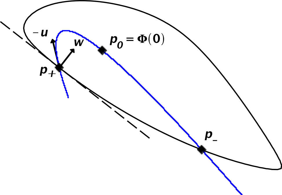
Consider a parametric polynomial curve $\mathcal{C}$ such that it has a non-empty intersection with a spectrahedron $S$ . Throughout, we consider only the real trace of $\mathcal{C}$ . Assume that the value of the parameter $t=0$ corresponds to a point $\bm{p}_{0}$ , that lies in $\mathcal{C}\cap S^{\circ}$ . Furthermore, assume that the segment of $\mathcal{C}$ on which $\bm{p}_{0}$ lies, intersects the boundary of $S$ transversally at two points, say $\bm{p}_{-}$ and $\bm{p}_{+}$ . The operation intersection computes the parameters, $t_{-}$ and $t_{+}$ , corresponding to these two points. Figure 2 illustrates this discussion and the pseudo-code of intersection appears in Algorithm 2.

To prove correctness and estimate the complexity we proceed as follows: As before (see also Equation 1), $S$ is the feasible region of linear matrix inequalities (LMI) $\bm{F}(\bm{x})\succeq 0$ . Consider the real trace of a polynomial curve $\mathcal{C}$ , with parameterization

\begin{array}[]{lllll}\Phi&:&\mathbb{R}&\rightarrow&\mathbb{R}^{n}\\ &&t&\mapsto&\Phi(t):=(p_{1}(t),\dots,p_{n}(t)),\end{array}

(3)

where $p_{i}(t)=\sum_{j=0}^{d_{i}}p_{i,j}t^{j}$ are univariate polynomials in $t$ of degree $d_{i}$ , for $i\in[m]$ . Also let $d=\max_{i\in[m]}\{d_{i}\}$ . If the coefficients of the polynomials are integers, then we further assume that the maximum coefficient’s bitsize is bounded by $\tau$ .

As $t$ varies over the real line, there may be several disjoint intervals, for which the corresponding segment of $\mathcal{C}$ lies in $S^{\circ}$ . We aim to compute the endpoints, $t_{-}$ and $t_{+}$ , of a maximal such interval containing $t=0$ . Let $\bm{p}_{0}=\Phi(0)$ ; by assumption it holds $\bm{F}(\Phi(0))=\bm{F}(\bm{p}_{0})\succ 0$ .

The input of intersection (Algorithm 2) is $\bm{F}$ , the LMI representation of $S$ , and $\Phi(t)$ , the polynomial parameterization of $\mathcal{C}$ . Its crux is a routine, pep, that solves a polynomial eigenvalue problem. The following lemma exploits this relation.

Input : An LMI

\bm{F}(\bm{x})\succeq 0

for a spectrahedron

S

and a parameterization

\Phi(t)

of a polynomial curve

\mathcal{C}

Require :

\Phi(0)\in S^{\circ}

Output :

{t_{-}},{t_{+}}

s.t.

\Phi({t_{-}}),\Phi({{t_{+}}})\in{\partial S}

T:=\{t_{1}\leq t_{2}\leq\cdots\leq t_{\ell}\}\leftarrow\textsc{pep}(\bm{F}(\Phi(t)))

; 5

{t_{-}}\leftarrow\max\{t\in T\,|\,t<0\}

; // max negative polynomial eigenvalue 6

{t_{+}}\leftarrow\min\{t\in T\,|\,t>0\}

; // min positive polynomial eigenvalue 7

return

t_{-},{t_{+}}

; 8

Algorithm 2

\textsc{intersection}(\bm{F},\Phi(t))

Lemma 2.3 (pep and $S\cap\mathcal{C}$ ).

Consider the spectrahedron $S=\{\bm{x}\in\mathbb{R}^{n}\,|\,\bm{F}(\bm{x})\succeq 0\}$ . Let $\Phi:\mathbb{R}\rightarrow\mathbb{R}^{n}$ be a parameterization of a polynomial curve $\mathcal{C}$ , such that $\Phi(0)\in S^{\circ}$ . Let $[t_{-},t_{+}]$ be the maximal interval containing $0$ , such that the corresponding part of $\mathcal{C}$ lies in ${S}$ . Then, $t_{-}$ , respectively $t_{+}$ , is the maximum negative, respectively minimum positive, polynomial eigenvalue of $\bm{F}(\Phi(t))\bm{x}=0$ , where $\bm{F}(\Phi(t))=\bm{B}_{0}+t\bm{B}_{1}+\cdots+t^{d}\bm{B}_{d}$ .

Proof.

The composition of $\bm{F}(\bm{x})$ and $\Phi(t)$ gives

\bm{F}(\Phi(t))=\bm{A}_{0}+p_{1}(t)\bm{A}_{1}+\cdots+p_{n}(t)\bm{A}_{n}.

(4)

We rewrite Expression (4) by grouping the coefficients for each $t^{i}$ , $i\in[d]$ , then

\bm{F}(\Phi(t))=\bm{B}_{0}+t\bm{B}_{1}+\cdots+t^{d}\bm{B}_{d},

(5)

where $\bm{B}_{k}=\sum_{j=0}^{n}p_{j,k}\,\bm{A}_{j}$ , for $0\leq k\leq d$ . We use the convention that $p_{j,k}=0$ , when $k>d_{j}$ .

For $t=0$ , it holds, by assumption, that $\bm{F}(\Phi(0))=\bm{B}_{0}\succ 0$ : point $\Phi(0)$ lies in the interior of $S$ . Actually, for any $\bm{x}\in S^{\circ}$ it holds $\bm{F}(\bm{x})\succ 0$ . On the other hand, if $\bm{x}\in{\partial S}$ , then $\bm{F}(\bm{x})\succeq 0$ . Our goal is to compute the maximal interval $[t_{-},t_{+}]$ that contains $0$ and for every $t$ in it, we have $\bm{F}(\Phi(t))\succeq 0$ .

Starting from point $\Phi(0)$ , by varying $t$ , we move on the trajectory that $\mathcal{C}$ defines (in both directions) until we hit the boundary of $S$ . When we hit ${\partial S}$ , matrix $\bm{F}(\Phi(t))$ is not strictly definite anymore. Thus, its determinant vanishes.

Consider the function $\theta:\mathbb{R}\rightarrow\mathbb{R}$ , where $\theta(t)=\det\bm{F}(\Phi(t))$ is a univariate polynomial in $t$ . If a point $\Phi(t)$ is on the boundary of the spectrahedron, then $\theta(t)=0$ . We opt to compute $t_{-}$ and $t_{+}$ , such that $t_{-}\leq 0\leq t_{+}$ and $\theta(t_{-})=\theta(t_{+})=0$ . At $t=0$ , $\theta(0)>0$ and the graph of $\theta$ is above the $t$ -axis. So $\mathcal{C}$ intersects the boundary when the graph of $\theta$ touches the $t$ -axis for the first time at $t_{1}\leq 0\leq t_{2}$ . It follows that $t_{-}=t_{1}$ and $t_{+}=t_{2}$ are the maximum negative and minimum positive roots of $\theta$ , or equivalently the corresponding polynomial eigenvalues of $\bm{F}(\Phi(t))$ . ∎

Lemma 2.4.

Algorithm 2, $\textsc{intersection}(\bm{F},\Phi(t))$ , uses $\widetilde{\mathcal{O}}((md)^{2.697}+md\lg{L})$ arithmetic operations in order to compute the intersection, up to precision $\epsilon=2^{-L}$ , of an LMI, $\bm{F}$ , consisting of $n$ matrices of dimension $m\times m$ with a parametric curve, $\Phi(t)$ , of degree $d$ .

Proof.

We have to construct PEP and solve it. Since $\Phi(t)$ has degree $d$ , then $\bm{F}(\Phi(t))=\bm{B}_{0}+t\bm{B}_{1}+\cdots+t^{d}\bm{B}_{d}$ is a PEP of degree $d$ . This construction costs $\mathcal{O}(dnm^{2})$ operations. The solving phase, using Lemma 2.1, requires $\widetilde{\mathcal{O}}((md)^{2.697}+md\lg{L})$ arithmetic operations and dominates the complexity bound of the algorithm. ∎

2.4 reflection

Input : An LMI

\bm{F}(\bm{x})\succeq 0

for a spectrahedron

S

and a parameterization

\Phi(t)

of a polynomial curve

\mathcal{C}

Require : (i)

\Phi(0)\in S^{\circ}

(ii)

\mathcal{C}

intersects

{\partial S}

transversally at a smooth point.

Output :

t_{+}

such that

\Phi(t_{+})\in{\partial S}

and the direction of the reflection,

\bm{s}_{+}

, at this point.

t_{-},t_{+}\leftarrow

intersection

(\bm{F},\Phi(t))

; 6

\bm{w}\leftarrow\nabla\det\bm{F}(\Phi(t_{+}))

; 7

\bm{w}\leftarrow\tfrac{\bm{w}}{\mathopen{\|}\bm{w}\mathclose{\|}}

; // Normalize

\bm{w}

\bm{s}_{+}\leftarrow\frac{d\Phi}{dt}(t_{+})-2\,\langle\nabla\frac{d\Phi}{dt}(t_{+}),\bm{w}\rangle\,\bm{w}

; 9

return

t_{+}

\bm{s}_{+}

; 10

Algorithm 3 reflection

(\bm{F},\Phi(t))

The reflection operation (Algorithm 3) takes as input an LMI representation, $\bm{F}$ , of a spectrahedron $S$ and a polynomial curve $\mathcal{C}$ , given by a parameterization $\Phi$ . Assume that $t=0$ corresponds to a point $\Phi(0)\in S^{\circ}\cap\mathcal{C}$ . Starting from $t=0$ , we increase $t$ along the positive real semi-axis. As $t$ changes, we move along the curve $\mathcal{C}$ through $\Phi(t)$ , until we hit the boundary of $S$ at the point $\bm{p}_{+}:=\Phi(t_{+})\in{\partial S}$ , for some $t_{+}>0$ . Then, a specular reflection occurs at this point with direction $\bm{s}_{+}$ ; this is the reflected direction. We output $t_{+}$ and $\bm{s}_{+}$ . Figure 2 depicts the procedure.

The boundary of $S$ , ${\partial S}$ , with respect to the Euclidean topology, is a subset of the real algebraic set $\{\bm{x}\in\mathbb{R}^{n}\,|\,\det(\bm{F}(\bm{x}))=0\}$ . The latter is a real hypersurface defined by one (determinantal) equation. For any $\bm{x}\in{\partial S}$ we have $\mathtt{rank}(\bm{F}(\bm{x}))\leq m-1$ . We assume that $\bm{p}_{+}=\Phi(t_{+})$ is such that $\mathtt{rank}(\bm{F}(\bm{p}_{+}))=m-1$ . The normal direction at a point $\bm{p}\in{\partial S}$ , is the gradient of $\det\bm{F}(\bm{p})$ .

We compute the reflected direction using the following formula

\bm{s}_{+}=\bm{u}-\tfrac{2}{|\bm{w}|^{2}}\langle\bm{u},\bm{w}\rangle\,\bm{w},

(6)

where $\bm{w}$ is the normalized gradient vector at the point $\Phi(t_{+})$ and $\bm{u}=\frac{d\Phi}{dt}(t_{+})$ is the direction of the trajectory at this point. We illustrate the various vectors in Figure 2.

Lemma 2.5 (Gradient of $\det\bm{F}(\bm{x})$ ).

Assume that $\bm{x}\in{\partial S}$ and the rank of the $m\times m$ matrix $\bm{F}(\bm{x})$ is $m-1$ . Then

\nabla\det(\bm{F}(\bm{x}))=c\cdot(\bm{v}^{\top}\bm{A}_{1}\bm{v},\cdots,\bm{v}^{\top}\bm{A}_{n}\bm{v}),

(7)

where $c=\frac{\mu(\bm{F}(\bm{x}))}{|\bm{v}|^{2}}$ , $\mu(\bm{F}(\bm{x}))$ is the product of the nonzero eigenvalues of $\bm{F}(\bm{x})$ , and $\bm{v}$ is a non-trivial vector in the kernel of $\bm{F}(\bm{x})$ . If $\mathtt{rank}(\bm{F}(\bm{x}))\leq m-2$ , then the gradient is the zero.

Proof.

From Lemma A.2:

\displaystyle\frac{\partial\det\bm{F}(\bm{x})}{\partial x_{k}}=\mathtt{Trace}\left(\bm{\bm{F}(\bm{x})}^{*}\bm{A}_{k}\right).

(8)

If $\mathtt{rank}(\bm{F}(\bm{x}))\leq-2$ , then $\bm{\bm{F}(\bm{x})}^{*}$ is the zero matrix. If we assume that $\mathtt{rank}(\bm{F}(\bm{x}))=m-1$ , then using Lemma A.3:

	$\displaystyle\mathtt{Trace}\left(\bm{\bm{F}(\bm{x})}^{*}\bm{A}_{k}\right)$	$\displaystyle=\mathtt{Trace}\left(\mu(\bm{F}(\bm{x}))\frac{\bm{v}\bm{u}^{\top}}{\bm{u}^{\top}\bm{v}}\bm{A}_{k}\right)$
		$\displaystyle=\frac{\mu(\bm{F}(\bm{x}))}{\bm{u}^{\top}\bm{v}}\cdot\mathtt{Trace}\left(\bm{v}\bm{u}^{\top}\bm{A}_{k}\right)=\frac{\mu(\bm{F}(\bm{x}))}{\bm{u}^{\top}\bm{v}}\cdot\bm{u}^{\top}\bm{A}_{k}\bm{v}.$

However, since $\bm{F}(\bm{x})$ is symmetric, we can choose $\bm{v}=\bm{u}$ , so:

\frac{\mu(\bm{F}(\bm{x}))}{\bm{u}^{\top}\bm{v}}\cdot\bm{u}^{\top}\bm{A}_{k}\bm{v}=\frac{\mu({\bm{F}(\bm{x}))}}{|\bm{v}|^{2}}\cdot\bm{v}^{\top}\bm{A}_{k}\bm{v}.

∎

The algorithm reflection exploits Lemma 2.5. Nevertheless, it is not necessary to perform all then computations that the lemma indicates. For example, because we will normalize the resulting vector and we do not need its actual direction (internal or external), we can omit the computation of $c$ . Moreover, the nonzero vector $\bm{v}$ , which satisfies $\bm{F}(\bm{p})\bm{v}=0$ , corresponds to the eigenvector w.r.t. the eigenvalue $t_{+}$ from the pep (Lemma 2.3). This is true because $\bm{p}=\Phi(t_{+})\in{\partial S}$ and thus $\det\bm{F}(\Phi(t_{+}))=0$ .

At this point we should note that we compute the eigenvalues of pep up to some precision. Since the matrix-vector multiplication is backward stable, a small perturbation on $\bm{v}$ does not affect the computation of each coordinate of $\nabla\det(\bm{F}(\bm{x}))$ [55, p. 104]. We quantify the accuracy of the computed $\nabla\det(\bm{F}(\bm{x}))$ using floating point arithmetic as follows:

Lemma 2.6.

The relative error of each coordinate of the gradient given in Lemma 2.5 when we compute it using floating point arithmetic with machine epsilon $\epsilon_{M}$ is $\mathcal{O}(\frac{\epsilon_{M}}{\sigma_{\max}(A_{i})})$ , for $i\in[n]$ , where $\sigma_{\max}$ is the largest singular value of $A_{i}$ .

Proof.

Let $A\in\mathbb{R}^{m\times m}$ be a symmetric matrix and consider the map $f:\bm{v}\mapsto\bm{v}^{T}A\bm{v}$ . The relative condition number of $f$ as defined in [55, p. 90] is

\displaystyle k(\bm{v})=\frac{||J(\bm{v})||}{||f(\bm{v})||/||\bm{v}||}=2\frac{||A\bm{v}||}{\bm{v}^{T}A_{i}\bm{v}}=2\frac{\sigma_{\max}(A)}{\sigma_{\max}^{2}(A)}=\frac{2}{\sigma_{\max}(A)},

where $J(\cdot)$ is the Jacobian of $f$ . According to Theorem 15.1 in [55, p. 111], since the matrix-vector multiplication is backward stable, the relative error of each coordinate in the gradient computation of Lemma 2.5 is $\mathcal{O}(\frac{\epsilon_{M}}{\sigma_{\max}(A_{i})})$ , for $1\leq i\leq n$ . ∎

Lemma 2.7.

Let $S$ be a spectrahedron represented by an LMI, $\bm{F}(\bm{x})$ , consisting of $n$ matrices of dimension $m\times m$ . Also let $\mathcal{C}$ be a parametric curve with parameterization $\Phi(t)$ , involving polynomials of degree at most $d$ . Algorithm 3, $\textsc{reflection}(\bm{F},\Phi(t))$ , computes the intersection, up to precision $\epsilon=2^{-L}$ , of $S$ with $\mathcal{C}$ , and the reflection of $\mathcal{C}$ at ${\partial S}$ , by performing $\widetilde{\mathcal{O}}((md)^{2.697}~+~md\lg{L}~+~dnm^{2})$ arithmetic operations.

Proof.

By inspecting Algorithm 3 we notice that the complexity of the algorithm depends on the construction of $\nabla\det(\bm{F}(\bm{x}))$ and the call to intersection.

To compute $\nabla\det(\bm{F}(\bm{x}))$ we just need to compute $(\bm{v}^{\top}\bm{A}_{1}\bm{v},\cdots,\bm{v}^{\top}\bm{A}_{n}\bm{v})$ . If we have already computed $\bm{v}$ , then this computation requires $\mathcal{O}(nm^{2})$ operations. The computation of the derivative of $\Phi(t)$ is straightforward, as $\Phi$ is a univariate polynomial. Taking into account the complexity of intersection, the total complexity for reflection is $\widetilde{\mathcal{O}}((md)^{2.697}+md\lg{L}+dnm^{2}+nm^{2})=\widetilde{\mathcal{O}}((md)^{2.697}~+~md\lg{L}~+~dnm^{2})$ . ∎

2.5 An example in 2D

Consider a spectrahedron $S$ in the plane (Figure 3), given by an LMI $\bm{F}(\bm{x})=\bm{A}_{0}+x_{1}\bm{A}_{1}+x_{2}\bm{A}_{2}$ . The matrices $\bm{A}_{i}$ , $0\leq i\leq 2$ , are in the appendix.

Starting from the point $\bm{p}_{0}=(-1,1)^{\top}$ , we walk along the line $L$ with parameterization: $\Phi(t)=\bm{p}_{0}+t\bm{u}$ , where $\bm{u}=(1.3,0.8)^{\top}$ . Then, intersection finds the intersection of $S$ with $L$ , by solving the degree one PEP, $(\bm{B}_{0}+t\bm{B}_{1})\bm{x}=0$ , where $\bm{B}_{0}=\bm{F}(\bm{p}_{0})$ and $\bm{B}_{1}=u_{1}\bm{A}_{1}+u_{2}\bm{A}_{2}$ . Acquiring $t_{-}=-0.8$ and $t_{+}=0.5$ , we obtain the intersection point $\bm{p_{1}}$ , which corresponds to $\bm{p}_{0}+t_{+}\bm{u}=(-0.3,1.4)^{\top}$ .

To compute the direction of the trajectory, immediately after we reflect on the boundary of $S$ at $\bm{p_{1}}$ , reflection computes

\bm{w}=\frac{\nabla\det\bm{F}(\Phi(t_{+}))}{|\nabla\det\bm{F}(\Phi(t_{+}))|}=(\bm{v}^{\top}\bm{A}_{1}\bm{v},\bm{v}^{\top}\bm{A}_{2}\bm{v})^{\top}=(-0.2,-1)^{\top},

(9)

where $\bm{v}$ is the eigenvector of $(\bm{B}_{0}+t\bm{B}_{1})\bm{x}=0$ , with eigenvalue $t_{+}$ . The reflected direction is $\bm{u^{\prime}}=\bm{u}-2\langle\bm{u},\bm{w}\rangle\,\bm{w}=(0.8,-1.3)^{\top}.$

3 Random walks

	per-step Complexity
W-HnR	$\mathcal{O}(m^{2.697}+m\lg{L}+nm^{2})$
W-CHnR	$\mathcal{O}(m^{2.697}+m\lg{L}+m^{2})$
W-Billard	$\widetilde{\mathcal{O}}(\rho(m^{2.697}+m\lg{L}+nm^{2}))$
W-HMC-r	$\widetilde{\mathcal{O}}(\rho((dm)^{2.697}+md\lg{L}+dnm^{2}))$

Table 1: The per-step complexity of the random walks in Section 3.

Using the basic geometric operations of Section 2, we implement and analyze three random walks for spectrahedra: Hit and Run (W-HnR), its variant Coordinate Directions Hit and Run (W-CHnR), Billiard Walk (W-Billard), and Hamiltonian Monte Carlo with reflections (W-HMC-r). In Table 1, we present the per-step arithmetic complexity for each random walk.

3.1 Hit and Run

W-HnR (Algorithm 4) is a random walk that samples from any probability distribution $\pi$ truncated to a convex body $K$ ; in our case a spectrahedron $S$ . We should mention that there exist bounds for its mixing time only when $\pi$ is log-concave distribution, for example the uniform distribution, which is $\widetilde{\mathcal{O}}(n^{3})$ .

At the $i$ -th step, W-HnR chooses uniformly at random a (direction of a) line $\ell$ , passing from its current position $\bm{p}_{i}$ . Let $\bm{p}_{1}$ and $\bm{p}_{2}$ be the intersection points of $\ell$ with $S$ . Let $\pi_{\ell}$ be the restriction of $\pi$ on the segment $[\bm{p_{2}},\bm{p_{2}}]$ . Then, we choose $\bm{p}_{i+1}$ from $[\bm{p_{1}},\bm{p_{2}}]$ w.r.t. the distribution $\pi_{\ell}$ .

Input : LMI

\bm{F}(\bm{x})\succeq 0

for a spectrahedron

S

& a point

\bm{p}_{i}

Require :

\bm{p}_{i}\in S

Output : The point

\bm{p}_{i+1}

of the

(i+1)

-th step of the walk.

BO (

\bm{F}

, interior point

\bm{p_{i}}

)

\bm{v}\leftarrow_{R}\mathcal{U}({\partial\mathcal{B}_{n}})

; // choose direction

\Phi(t):=\bm{p}_{i}+t\bm{v}

; // define trajectory
5

{t_{-}},{t_{+}}

\leftarrow

intersection (

\bm{F},\Phi(t)

); 6

\bm{p}_{i+1}\leftarrow_{R}[\bm{p}_{i}+{t_{-}}\bm{v},\ \bm{p}_{i}+{t_{+}}\bm{v}]

w.r.t.

\pi_{\ell}

; 7

return

\bm{p}_{i+1}

; 9

Algorithm 4 Hit-and-Run_Walk (W-HnR)

Lemma 3.1.

The per-step complexity of W-HnR is $\widetilde{\mathcal{O}}(m^{2.697}+m\lg{1/\epsilon}+nm^{2})$ .

Proof.

The per-step complexity of W-HnR is dominated by the intersection, which requires $\mathcal{O}(nm^{2})$ operations for the construction of the pep and $\widetilde{\mathcal{O}}(m^{2.697}+m\lg{1/\epsilon})$ for solving it; in the case where we want to approximate the intersection point up to a factor or $\epsilon=2^{-L}$ (Lemma 2.4). ∎

There is also a variation of W-HnR, the coordinate directions Hit and Run (W-CHnR) [50]. This walk chooses the direction vector randomly and uniformly among the vector basis { $\bm{e}_{i},\ i\in[n]\}$ . In W-CHnR, for every step aside the first, the construction of the pep takes $\mathcal{O}(m^{2})$ operations, and the complexity does not depend on the dimension $n$ . The reason for this improvement is that to build the pep, $\bm{F}(\bm{p}_{i}+t\bm{e}_{j})=\bm{F}(\bm{p}_{i})+t\bm{A}_{j}$ , we can obtain the value of $\bm{F}(\bm{p}_{i})$ from $\bm{F}(\bm{p}_{i})=\bm{F}(\bm{p}_{i-1})+\hat{t}\bm{A}_{k}$ , assuming that at the previous step we have chosed $\bm{e}_{k}$ as direction. There is no theoretical mixing time for W-CHnR.

3.2 Billiard walk

W-Billard [45], Algorithm 5, samples a convex body $K$ under the uniform distribution; no theoretical results for its mixing time exist. At $i$ -th step, being at position $\bm{p}_{i}$ , it chooses uniformly a direction vector $\bm{v}$ and a number $\ell$ , where $\ell=-\tau\ln\eta$ and $\eta\sim U(0,1)$ . Then, it moves at the direction of $\bm{v}$ for distance $\ell$ . If during the movement, it hits the boundary without having covered the required distance $\ell$ , then it continues on a reflected trajectory. If the number of reflections exceeds a bound $\rho$ , it stays at $\bm{p}_{i}$ . In [45] they experimentally conclude that W-Billard mixes faster when $\tau\approx diam(K)$ , where $diam(K)$ is the diameter of $K$ .

Input : An LMI

\bm{F}(\bm{x})\succeq 0

for a spectrahedron

S

, a point

\bm{p_{i}}

, the diameter

\tau

S

and a bound

\rho

on the number of reflections.

Require :

\bm{p}_{i}\in S

Output : The point

\bm{p}_{i+1}

of the

(i+1)

-th step of the walk.

\ell\leftarrow-\tau\ln\eta

;

\eta\leftarrow_{R}\mathcal{U}((0,1))

; // choose length

\bm{v}\leftarrow_{R}\mathcal{U}({\partial\mathcal{B}_{n}})

; // choose direction

\bm{p}\leftarrow\bm{p}_{i}

; 5

do 7

\Phi(t):=\bm{p}+t\bm{v}

; // define trajectory

t_{+},\bm{s}_{+}

\leftarrow

reflection (

\bm{F},\Phi(t)

); 8

\hat{t}\leftarrow\min\{t_{+},\ell\}

;

\bm{p}\leftarrow\Phi(\hat{t})

; 9

if $\overline{t}<\ell$ then

\bm{v}\leftarrow

\bm{s}_{+}

; 10

\ell\leftarrow\ell-\hat{t}

; while $\ell>0$ ; 11

if $\#\{\text{reflections}\}>\rho$ then return

\bm{p_{i+1}}=\bm{p_{i}}

; 12

return

\bm{p}_{i+1}=\bm{p}

Algorithm 5 Billiard_Walk (W-Billard)

Lemma 3.2.

The per-step complexity of W-Billard is $\widetilde{\mathcal{O}}(\rho(m^{2.697}+m\lg{L}+nm^{2}))$ , where $\rho$ is the number of reflections.

Proof.

The per-step complexity of W-Billard is dominated by the reflection, which requires $\widetilde{\mathcal{O}}(m^{2.697}+m\lg{L}+nm^{2})$ arithmetic operations (Lemma 2.7), when we want to approximate the intersection point up to a factor of $2^{-L}$ . Since we allow at most $\rho$ reflections per step, the total complexity becomes $\widetilde{\mathcal{O}}(\rho(m^{2.697}+m\lg{L}+nm^{2}))$ . ∎

3.3 Hamiltonian Monte Carlo with Reflections

Input : An LMI

\bm{F}(\bm{x})\succeq 0

representing a spectrahedron

S

, a point

\bm{p}_{i}

, the diameter

\tau

S

and a bound

\rho

to the number of reflections.

Require :

\bm{p}_{i}\in S

Output : The point

\bm{p}_{i+1}

of the

(i+1)

-th step of the walk.

\ell\leftarrow\tau\eta

;

\ \eta\leftarrow_{R}\mathcal{U}((0,1))

; // choose length

\bm{v}\leftarrow_{R}\mathcal{N}(0,I_{n})

; // choose direction
5

do 6

Compute trajectory

\Phi(t)

from ODE (10); 7

{t_{+}},\bm{s}_{+}

\leftarrow

reflection (

\bm{F},\Phi(t)

); 8

\hat{t}\leftarrow\min\{{t_{+}},\ell\}

;

\bm{p}\leftarrow\Phi(\hat{t})

;

\bm{v}\leftarrow

\bm{{s}}

;

\ell\leftarrow\ell-\hat{t}

; while $\ell>0$ ; 9

if $\#\ \{\text{reflections}\}>\rho$ then return

\bm{p}_{i+1}=\bm{p}_{i}

; 10

return

\bm{p}_{i+1}=\bm{p}

; 12

Algorithm 6 HMC_w_reflection (W-HMC-r)

Hamiltonian Monte Carlo (HMC), can be used to sample from any probability distribution $\pi$ . Our focus lies again on the log-concave distributions, that is $\pi(\bm{x})\propto e^{-\alpha f(\bm{x})}$ . We exploit the setting in [34] as they approximate the Hamiltonian trajectory with a polynomial curve. In this setting, if we assume that $f$ is a strongly convex function, then the mixing time of HMC is $\mathcal{O}(k^{1.5}\log(n/\epsilon))$ , where $\kappa$ is the condition number of $\nabla^{2}f$ [34]. If we truncate $\pi$ by considering its restriction in a convex body, then we can use boundary reflections (W-HMC-r), as in Algorithm 6, to ensure that the random walk converges to the target distribution [15]; however, in this case the mixing time is unclear.

The Hamiltonian dynamics behind HMC operate on a $n$ -dimensional position vector $\bm{p}$ and a $n$ -dimensional momentum $\bm{v}$ . So the full state space has $2n$ dimensions. The system is described by a function of $\bm{p}$ and $\bm{v}$ known as the Hamiltonian,

H(\bm{p},\bm{v})=U(\bm{p})+K(\bm{v})=f(\bm{p})+\frac{1}{2}|\bm{v}|^{2}.

To sample from $\pi$ , one has to solve the following system of Ordinary Differential Equations (ODE):

\begin{split}\frac{d\bm{p}}{dt}=\frac{\partial H(\bm{p},\bm{v})}{\partial\bm{v}}\\ \frac{d\bm{v}}{dt}=-\frac{\partial H(\bm{p},\bm{v})}{\partial\bm{p}}\end{split}\quad\Rightarrow\quad\left\{\begin{array}[]{lll}\frac{d\bm{p}(t)}{dt}=\bm{v}(t)\\ \\ \frac{d\bm{v}(t)}{dt}=-\alpha\nabla f(\bm{p})\\ \end{array}\right..

(10)

If $\pi(\bm{x})$ is a log-concave density, then we can approximate the solution of the ODE with a low degree polynomial trajectory [34], using the collocation method. A degree $d=\mathcal{O}(1/\log(\epsilon))$ suffices to obtain a polynomial trajectory with error $\mathcal{O}(\epsilon)$ , for a fixed time interval, while we perform just $\widetilde{\mathcal{O}}(1)$ evaluations of $\nabla f(\bm{x})$ .

HMC at the $i$ -th step uniformly samples a step $\ell$ from a proper interval to move on the trajectory implied by ODE (10), choses $\bm{v}$ randomly from $\mathcal{N}(0,I_{n})$ , and updates $\bm{p}$ using the ODE in (10), for $t\in[0,\ell]$ . When $\pi$ is truncated in a convex body, then W-HMC-r fixes an upper bound $\rho$ on the number of reflections and reflects a polynomial trajectory as we describe in Section 2.4.

Each step of W-HMC-r, when $\pi(x)$ is a log-concave density truncated by $S$ , costs $\widetilde{\mathcal{O}}(\rho((dm)^{2.697}+md\lg{L}+dnm^{2}))$ , if we approximate the intersection points up to a factor $2^{-L}$ , where $d$ is the degree of the polynomial that approximates the solution of the ODE (10).

Lemma 3.3.

The per-step complexity of W-HMC-r is $\widetilde{\mathcal{O}}(\rho((dm)^{2.697}+md\lg{L}+dnm^{2}))$ , where $\rho$ is the number of reflections.

4 Applications and experiments

This section demonstrates and compares the algorithms of Section 3 and the efficiency of our software on three applications that rely on sampling from spectrahedra.

We call walk length the number of the intermediate points that a random walk visits before producing a single sample. The longer the walk length of a random walk is, the smaller the distance of the current distribution to the stationary (target) distribution becomes. Typically we choose a sufficiently large length for the first sample, this procedure is often called "burning".

Our code is parameterized by the floating point precision of the computations. We use Eigen [25] for basic linear algebra operations, such as Cholesky decomposition and matrix multiplication. For eigenvalue computations, we employ Spectra [51], which is based on Eigen and offers crucial optimizations. First, it solves generalized eigenvalue problems of special structure; that is $(B_{0}-\lambda B_{1})v=0$ , when $B_{0}$ is positive semidefinite and $B_{1}$ symmetric. This operation is encountered when W-Billard or W-HnR call intersection. Second, it offers directly the computation of the largest eigenvalue which corresponds to $t_{+}$ after a simple transformation. Finally, Spectra provides $\sim 20$ x speedup over the default eigenvalue computation by Eigen. To the best of our knoledge, our software is the first that can sample efficiently from spectrahedra and estimates volumes up to a few hundred dimensions. It is accessible on github.²² 2 https://github.com/GeomScale/volume_approximation/tree/sample_spectrahedra

For our experiments, we generate random spectrahedra following [18]. In particular, to construct the LMI of Equation (1) we set $A_{0}$ to be positive semidefinite, i.e., $A_{0}=ZZ^{T}+I_{m}$ , where we pick the elements of $Z\in\mathbb{R}^{m\times m}$ uniformly at random from $[0,1]$ . Then, for $A_{i},\ i=1,\dots,n$ we set,

A_{i}=\left[\begin{array}[]{cc}\tilde{Q}&0\\ 0&-\tilde{Q}\end{array}\right],\ \tilde{Q}=Q+Q^{T},

where we pick the elements of $Q\in\mathbb{R}^{(m/2)\times(m/2)}$ uniformly at random from $[-1,1]$ . We performed all the experiments on PC with Intel Core i7-6700 3.40GHz $\times$ 8 CPU and 32GB RAM.

4.1 Volume computation

We use the geometric operations (Section 2) and the random walks (Section 3) to compute the volume $\mbox{vol}(S)$ of spectrahedron $S$ . Our implementation approximates $\mbox{vol}(S)$ within relative error $0.1$ with high probability in a few minutes, for dimension $n=100$ .

A typical randomized algorithm for volume approximation exploits a Multiphase Monte Carlo (MMC) technique, which reduces volume approximation of convex body $S$ to computing a telescoping product of ratios of integrals over $S$ . In particular, for any sequence of functions $\{f_{0},\ \dots,f_{k}\}$ , where $f_{i}:\mathbb{R}^{n}\rightarrow\mathbb{R}$ , we have:

\mbox{vol}(S)=\int_{S}1dx=\int_{S}f_{k}(x)dx\frac{\int_{S}f_{k-1}(x)dx}{\int_{S}f_{k}(x)dx}\cdots\frac{\int_{S}1dx}{\int_{S}f_{0}(x)dx}.

(11)

Notice that $\frac{\int_{P}f_{i-1}(x)dx}{\int_{P}f_{i}(x)dx}=\int_{P}\frac{f_{i-1}(x)}{f_{i}(x)}\frac{f_{i}(x)}{\int_{P}f_{i}(x)dx}dx$ . To estimate each ratio of integrals, we sample $N$ points from a distribution proportional to $f_{i}$ and, we use the unbiased estimator $\frac{1}{N}\sum_{j=1}^{N}\frac{f_{i-1}(x_{j})}{f_{i}(x_{j})}$ . To exploit Equation (11) we have to (i) fix the sequence such that $k$ is as small as possible, (ii) select $f_{i}$ ’s such that we can compute efficiently each integral ratio, and (iii) compute $\int_{P}f_{k}(x)dx$ . The best theoretical result of [16] fixes a sequence of spherical Gaussians $\{f_{0},\ \dots,f_{k}\}$ with the mode being in $S$ , parameterized by the variance. The overall complexity is $\widetilde{\mathcal{O}}(n^{3})$ membership calls. The implementation in [17] is based on this algorithm but handles only convex polytopes in H-representation as it requires the facets of the polytope and an inscribed ball to fix the sequence of Gaussians. Both the radius of the inscribed ball and the number of facets strongly influence the performance of the algorithm. So, it cannot handle efficiently the case of convex bodies without a facet description, e.g., zonotopes [17], as it results a big sequence of ratios that spoil practical efficiency.

$S$ - $n$ - $m$	$\mu\pm t_{\alpha,\nu-1}\frac{s}{\sqrt{\nu}}$	$Points$	$Time\ (sec)$
$S$ - $40$ - $40$	$(1.34\pm 0.12)$ e-06	9975.2	6.7
$S$ - $60$ - $60$	$(1.23\pm 0.11)$ e-20	20370.9	28.5
$S$ - $80$ - $80$	$(4.24\pm 0.26)$ e-33	31539.1	124.4
$S$ - $100$ - $100$	$(1.21\pm 0.10)$ e-51	52962.7	362.3

Table 2: (Volume of spectrahedra) For each $S$ - $n$ - $m$ we run $\nu=10$ experiments; $m$ is the matrix dimension in LMI and $n$ the ambient dimension. $\mu$ stands for the average volume, $s$ for the standard deviation; we give a confidence interval with level of confidence $\alpha=0.05$ ; $t_{\alpha,\nu-1}$ is the critical value of student’s distribution with $\nu-1$ degrees of freedom. $Points$ denotes the average number of points generated and $Time$ the average runtime in seconds. For all the above we set the error parameter $e=0.1$ .

Our approach is to consider the $f_{i}$ ’s as a sequence of indicator functions of concentric balls centered in $S$ , as in [21]. In particular, let $f_{k}$ and $f_{0}$ be the indicator functions of $r\mathcal{B}_{n}$ and $R\mathcal{B}_{n}$ respectively, while $r\mathcal{B}_{n}\subseteq S\subseteq R\mathcal{B}_{n}$ and $S_{i}=(2^{(k-i)/n}r\mathcal{B}_{n})\cap S$ for $i=0,\dots,k$ . Thus, it suffices to compute $\mbox{vol}(r\mathcal{B}_{n})$ and apply the following:

\mbox{vol}(S)=\mbox{vol}(S_{k})\frac{\mbox{vol}(S_{k-1})}{\mbox{vol}(S_{k})}\cdots\frac{\mbox{vol}(S_{0})}{\mbox{vol}(S_{1})},\quad k=\lceil n\lg(R/r)\rceil.

(12)

Furthermore, we employ the annealing schedule from [12] to minimize $k$ , without computing neither an enclosed ball $r\mathcal{B}_{n}$ nor an enclosing ball $R\mathcal{B}_{n}$ of $S$ . We do so by probabilistically bounding each ratio of Equation (12) in an interval $[r,r+\delta]$ , which is given as input. To approximate each ratio of volumes, we sample uniformly distributed points from $S_{i}$ and count points in $S_{i-1}$ . We follow the experimental results of Section 4.2 and use W-Billard which mixes faster than W-HnR.

Table 2 reports the average volume, runtime, number of points generated for each $S$ - $n$ - $m$ over $10$ trials. We also compute a $95\%$ confidence interval for the volume. Notice that for all cases the extreme values of each interval imply an error $\leq 0.1$ , which was the requested error. For $n=40$ just a few seconds suffice to approximate the volume and for $n=100$ our implementation takes a few minutes.

4.2 Expected value of a function

Randomized algorithms are commonly used for problems in robust control analysis to overcome the (worst case) hardness, especially in probabilistic robustness [6, 29, 53, 11]. A central problem is to approximate the integral of a function over a spectrahedron, e.g. [10, 48] and thus uniform sampling is of particular interest. To put our experiments into perspective, we present experiment up to $n=200$ , while in [10] and [11] they use only W-HnR for experiments in $n\leq 10$ .

Our goal is to compute the expected value of a function $f:\mathbb{R}^{n}\rightarrow[0,1]$ , with respect to the measure given by the uniform distribution $\pi$ over $S$ , i.e., $I=\int_{S}f(x)\pi(x)dx$ . A standard approach is the Monte Carlo method, which suggests to sample $N$ independent samples from $\pi$ . Then,

\hat{\mathbb{E}}_{N}[f]=\frac{1}{N}\sum_{i=1}^{N}f(x_{i})

is an unbiased estimator for $I$ . We employ the random walks of Section 3 to sample uniformly distributed points from $S$ (i.e., W-HnR, W-CHnR, and W-Billard) and we experimentally compare their efficiency. It turns out that W-Billard mixes much faster and results to better accuracy (see Figures 5 & 6). This observation agrees with the experiments on the rate of convergence for W-HnR and W-Billard in [45]. To come to a decisive conclusion we need to perform a more detailed practical study on the mixing time of these random walks; we leave this study as future work.

The variance of an estimator is a crucial as it bounds the approximation error. Using Chebyshev’s inequality and [37], we have

Prob[|\hat{\mathbb{E}}_{N}[f]-\mathbb{E}[f]|\leq\epsilon]\leq\frac{var(\hat{\mathbb{E}}_{N}[f])}{\epsilon^{2}}\leq\frac{4M_{\epsilon}}{N\epsilon^{2}},

(13)

where $M_{\epsilon}$ is the mixing time of the random walk one uses to sample “ $\epsilon$ close" to the uniform distribution from $S$ . Thus, for fixed $N$ and $\epsilon$ , the smaller the mixing time of the random walk is, the smaller the variance of estimator $\hat{\mathbb{E}}_{N}[f]$ and hence, the better the approximation. We estimate $I$ when $f:=1(S\cap H)$ , where $H$ is the union of two half-spaces $H:=\{x\ |\ cx\leq b_{1}\ \text{ or }\ cx\geq b_{2}\}$ , where $b_{2}>b_{1}$ and $1(\cdot)$ is the indicator function. Note that $I=\mbox{vol}(S\cap H)/\mbox{vol}(S)$ . To estimate it we sample approximate uniformly distributed points from $S$ and we count the number of points that lie in $S\cap H$ .

walk length	$1$	$5$	$10$	$20$	$30$	$40$	$50$
$S$ - $100$ - $100$	1.4	3.2	7.7	9.5	16.1	21.4	28.2
$S$ - $200$ - $200$	16.2	75.7	148	303	443	584	722

Table 3: Average time in sec to sample $200$ points with W-Billard from $10$ random spectrahedra $S$ - $n$ - $m$ ; $n$ for the dimension that $S$ - $n$ - $m$ lies; $m$ for the dimension of the matrix in LMI.

We estimate two functions $f_{1},\ f_{2}$ with $\mathbb{E}[f_{1}]=0.0993$ and $\mathbb{E}[f_{2}]=0.5880$ in dimension $n=50$ and for various walk lengths. For each walk length we sample $N=200$ points and we repeat $M=20$ times. Then, for each $N$ -set we compute $\frac{1}{N}\sum_{i=1}^{N}f(x_{i})$ and we take the average and the standard deviation (st.d.) over $M$ . Figures 5, & 6 illustrates these values, while the walk length increases. Notice that the st.d. is much smaller and the approximation more stable when W-Billard is used compared to both W-HnR and W-CHnR. As W-Billard mixes faster, we report in Table 3 the average time our software needs to sample $N=200$ points for various walk lengths for W-Billard in $n=100,\ 200$ . The average time to generate a point is $\approx 0.3$ and $\approx 7.2$ milliseconds respectively.

4.3 Sampling from non-uniform distributions

The random walks of Section 3 open a promising avenue for approximating the optimal solution of a semidefinite program, that is

\min\langle\bm{c},\bm{x}\rangle,\ \text{subject to }\bm{x}\in S.

(14)

We parameterize the optimization algorithm in [27] with the choice of random walk and demonstrate that its efficiency relies heavily on the sampling method. We perform experiments with W-HMC-r and W-HnR, as both can sample from the distribution the algorithm requires. Deterministic approximations to the optimal solutions of these tests, were acquired via the SDPA library [57].

The strategy to approximate the optimal solution $\bm{x}^{*}$ of Equation (14), is based on sampling from the Boltzmann distribution, i.e., $\pi(\bm{x})\propto e^{-\bm{c}\bm{x}/T}$ , truncated to $S$ . The scalar $T$ , is called temperature. As the temperature $T$ diminishes, the mass of $\pi$ tends to concentrate around its mode, which is $\bm{x}^{*}$ . Thus, one could obtain a uniform point using the algorithm in [38], and then use it as a starting point to sample from $\pi_{0}\propto e^{-cx/T_{0}}$ , where $T_{0}=R$ and $S\subseteq R\mathcal{B}_{n}$ . Then, the cooling schedule $T_{i+1}=T_{i}(1-1/\sqrt{n})$ guarantees that a sample from $\pi_{i}$ yields a good starting point for $\pi_{i+1}$ . After $\widetilde{\mathcal{O}}(\sqrt{n})$ steps the temperature will be low enough, to sample a point within distance $\epsilon$ from $\bm{x}^{*}$ with high probability.

In [27], they use only W-HnR. We also employ W-HMC-r. To sample from Boltzmann distributions with W-HMC-r, at each step, starting from $\bm{p_{i}}$ and with momenta $\bm{v_{i}}$ , the ODE of Equation (10) becomes

\frac{d^{2}}{dt^{2}}\bm{p}(t)=-\frac{\bm{c}}{T},\ \frac{d}{dt}\bm{p}(0)=\bm{v_{i}},\ \bm{p}(0)=\bm{p_{i}}.

(15)

Its solution is the polynomial $\bm{p}(t)=-\frac{\bm{c}}{2T}t^{2}+\bm{v_{i}}t+\bm{p_{i}}$ , which is a parametric representation of a polynomial curve, see Equation (3).

$S$ - $n$ - $m$	W-HMC-r	W-HnR $W_{1}$	W-HnR $W_{2}$
$S$ - $30$ - $30$	$20.1$ / $2.9$ / $0$	$184.3$ / $3.4$ / $1$	$52.1$ / $5.2$ / $0$
$S$ - $40$ - $40$	$24.6$ / $7.9$ / $0$	$223.3$ / $9.9$ / $2$	$61.9$ / $17.1$ / $0$
$S$ - $50$ - $50$	$29.2$ / $12.7$ / $0$	$251.2$ / $22.3$ / $3$	$72.3$ / $44.6$ / $0$
$S$ - $60$ - $60$	$32.8$ / $24.32$ / $0$	$272.7$ / $41.1$ / $3$	$81.5$ / $98.9$ / $0$

Table 4: The average $\#$ iteration / runtime / failures over $10$ generated $S$ - $n$ - $m$ , to achieve relative error $\epsilon\leq 0.05$ . The walk length is one for W-HMC-r and $W_{1}=4\sqrt{n}$ and $W_{2}=4n$ for W-HnR. With "failures" we count the number of times the method fails to converge. Also $m$ is the dimension of the matrix in LMI and $n$ is the dimension that $S$ - $n$ - $m$ lies.

In Table 4 we follow the cooling schedule described, after setting $T_{0}\approx R$ and sampling the first uniform point with W-Billard. We give the optimal solution as input and we stop dropping $T$ when an error $\epsilon\leq 0.05$ is achieved. Even in the case when the walk length is set equal to one, W-HMC-r still converges to the optimal solution. To the best of our knowledge, this is the first time that a randomized algorithm, which is based on random walks, is functional even when the walk length is set to one. On the other hand, we set the walk length of W-HnR $\mathcal{O}(\sqrt{n})$ or $\mathcal{O}(n)$ in our experiments. Notice that for the smaller walk length, its runtime decreases, but the method becomes unstable, as it sometimes fails to converge. For both cases its runtime is worse than that of W-HMC-r.

Acknowledgements

ET is partially supported by ANR JCJC GALOP (ANR-17-CE40-0009), the PGMO grant ALMA, and the PHC GRAPE.

Appendix A Additional proofs

To prove lemma 2.5 we will need the following lemmas.

Lemma A.1 (Partial Derivative of Determinant).

Let $\bm{A}$ be a symmetric $m\times m$ matrix. Then

\frac{\partial\det\bm{A}}{\partial A_{ij}}=c_{ij}

where $c_{ij}$ the cofactor of $A_{ij}$ .

Proof.

From Laplace expansion:

\det\bm{A}=\sum\limits_{j=1}^{m}A_{ij}c_{ij}

Notice that $c_{1j},\cdots,c_{mj}$ are independent of $A_{ij}$ , so we have

\frac{\partial\det\bm{A}}{\partial A_{ij}}=c_{ij}

∎

Lemma A.2.

Let $\bm{F}(\bm{x})=\bm{A}_{0}+x_{1}\bm{A}_{1}+\cdots+x_{n}\bm{A}_{n}$ . Then

\frac{\partial\det\bm{F}(\bm{x})}{\partial x_{k}}=\mathtt{Trace}\left(\bm{\bm{F}(\bm{x})}^{*}\bm{A}_{k})\right)

Proof.

The function $\det\bm{F}(\bm{x})$ is the composition of $\det\bm{A}$ and $\bm{A}=\bm{F}(\bm{x})$ , so from Lemma A.1 and the chain rule:

\frac{\partial\det\bm{F}(\bm{x})}{\partial x_{k}}=\sum\limits_{i=1}^{m}\sum\limits_{j=1}^{m}\frac{\partial\det\bm{F}}{\partial\bm{F}_{ij}}\cdot\frac{\partial\bm{F}_{ij}}{\partial x_{k}}=\sum\limits_{i=1}^{m}\sum\limits_{j=1}^{m}c_{ij}A^{k}_{ij}=\mathtt{Trace}\left(\bm{\bm{F}(\bm{x})}^{*}\bm{A}_{k}\right)

where $A^{k}_{ij}$ the $ij$ -th element of matrix $\bm{A}_{k}$ ∎

Lemma A.3 (Adjoint Matrix of $\bm{A}$ ).

Let $\bm{A}$ be a $m\times m$ matrix of rank $r(\bm{A})=m-1$ . Then

\bm{A}^{*}=\mu(\bm{A})\frac{\bm{v}\bm{u}^{\top}}{\bm{u}^{\top}\bm{v}}

where $\mu(\bm{A})$ is the product of the $m-1$ non-zero eigenvalues of $\bm{A}$ , and $\bm{x}$ and $\bm{y}$ satisfy $\bm{A}\bm{v}=\bm{A}^{\top}\bm{u}=\bm{0}$ (see chapter 3.2 in [40]).

Appendix B Matrices of the Example

The spectrahedron was randomly generated as in [18]. Due to space considerations, the entries of the matrices are rounded to the first decimal.

\bm{A_{0}}=\begin{bmatrix}16.7&3.7&12.3&8.7&5.1&10.4\\ 3.7&9.4&2.3&4&-2.3&-1\\ 12.3&2.3&26.8&18.7&7.1&16.7\\ 8.7&4&18.7&20&3.7&12.3\\ 5.1&-2.3&7.1&3.7&6.1&5.4\\ 10.4&-1&16.7&12.3&5.4&18.7\end{bmatrix}

(16)

\bm{A_{1}}=\begin{bmatrix}0.5&-0.4&2.7&0&0&\\ -0.4&1.4&-0.2&0&0&0\\ 2.7&-0.2&1.7&0&0&0\\ 0&0&0&0.5&-0.4&2.7\\ 0&0&0&-0.4&1.4&-0.2\\ 0&0&0&2.7&-0.2&1.7\end{bmatrix}

(17)

\bm{A_{2}}=\begin{bmatrix}2.6&-0.1&3&0&0&0\\ -0.1&1&-0.1&0&0&0\\ 3&-0.1&-1&0&0&0\\ 0&0&0&2.6&-0.1&3&\\ 0&0&0&-0.1&1&-0.1\\ 0&0&0&3&-0.1&-1\end{bmatrix}

(18)

References

[1] H. M. Afshar and J. Domke. Reflection, Refraction, and Hamiltonian Monte Carlo. In Proc. 28th NeurIPS, pages 3007--3015, Cambridge, MA, USA, 2015. MIT Press.
[2] D. Armentano and C. Beltrán. The polynomial eigenvalue problem is well conditioned for random inputs. SIMAX, 40(1):175–193, 2019.
[3] C. Beltrán and K. Kozhasov. The real polynomial eigenvalue problem is well conditioned on the average. J. Foundations of Computational Math., pages 1–19, 2019.
[4] M. Berhanu. The polynomial eigenvalue problem. PhD thesis, University of Manchester, 2005.
[5] M. Betancourt. A conceptual introduction to Hamiltonian Monte Carlo. arXiv preprint arXiv:1701.02434, 2017.
[6] V. D. Blondel and J. N. Tsitsiklis. A survey of computational complexity results in systems and control. Automatica, 36(9):1249–1274, 2000.
[7] J.-D. Boissonnat and M. Teillaud. Effective computational geometry for curves and surfaces. Springer, 2006.
[8] P. Breiding, K. Kozhasov, and A. Lerario. Random spectrahedra. SIAM J. Optimization, 29(4):2608–2624, 2019.
[9] B. Büeler, A. Enge, and K. Fukuda. Exact Volume Computation for Polytopes: A Practical Study. In G. Kalai and G. M. Ziegler, editors, Polytopes — Combinatorics and Computation, DMV Seminar, pages 131–154. Birkhäuser, Basel, 2000.
[10] G. Calafiore. Random walks for probabilistic robustness. In Proc. CDC, volume 5, pages 5316–5321. IEEE, 2004.
[11] G. Calafiore and M. Campi. Robust convex programs: Randomized solutions and applications in control. In Proc. CDC, volume 3, pages 2423–2428. IEEE, 2003.
[12] A. Chalkis, I. Z. Emiris, and V. Fisikopoulos. Practical volume estimation by a new annealing schedule for cooling convex bodies. arXiv preprint arXiv:1905.05494, 2019.
[13] A. Chalkis, V. Fisikopoulos, P. Repouskos, and E. Tsigaridas. Sampling the feasible sets of SDPs and volume approximation. poster version in ISSAC 2020, to appear in ACM Communications in Computer Algebra, 2020.
[14] Y. Chen, R. Dwivedi, M. J. Wainwright, and B. Yu. Vaidya walk: A sampling algorithm based on the volumetric barrier. In 2017 55th Annual Allerton Conference on Communication, Control, and Computing (Allerton), pages 1220–1227, Oct 2017.
[15] A. Chevallier, S. Pion, and F. Cazals. Hamiltonian Monte Carlo with boundary reflections, and application to polytope volume calculations. Research Report RR-9222, INRIA, Sophia-Antipolis, France, Nov. 2018.
[16] B. Cousins and S. Vempala. Bypassing KLS: Gaussian cooling and an ${O}^{*}(n^{3})$ volume algorithm. In Proc. ACM Symposium Theory of computation (STOC), pages 539–548, 2015.
[17] B. Cousins and S. Vempala. A practical volume algorithm. Mathematical Programming Computation, 8, June 2016.
[18] F. Dabbene, P. Shcherbakov, and B. T. Polyak. A randomized cutting plane method with probabilistic geometric convergence. SIAM J. Optimization, 20:3185–3207, 2010.
[19] J.-P. Dedieu and F. Tisseur. Perturbation theory for homogeneous polynomial eigenvalue problems. Linear algebra & Appl., 358(1-3):71–94, 2003.
[20] M. Dyer, A. Frieze, and R. Kannan. A random polynomial-time algorithm for approximating the volume of convex bodies. J. ACM, 38(1):1–17, 1991.
[21] I. Emiris and V. Fisikopoulos. Practical polytope volume approximation. ACM Trans. Math. Soft., 44(4):38:1–38:21, 2018. Prelim. version: Proc. SoCG, 2014.
[22] I. Emiris, F. Sottile, and T. Theobald, editors. Nonlinear computational geometry, volume 151 of I.M.A. volumes in Math & its Applications. Springer, Berlin, Oct. 2010.
[23] I. Z. Emiris, B. Mourrain, and E. Tsigaridas. Separation bounds for polynomial systems. J. Symbolic Computation, 2019.
[24] E. Gryazina and B. Polyak. Random sampling: Billiard walk algorithm. European J. Operational Research, 238, 11 2012.
[25] G. Guennebaud, B. Jacob, et al. Eigen v3, 2010. http://eigen.tuxfamily.org.
[26] D. Henrion, J. B. Lasserre, and C. Savorgnan. Approximate volume and integration for basic semialgebraic sets. SIAM review, 51(4):722–743, 2009.
[27] A. T. Kalai and S. Vempala. Simulated annealing for convex optimization. Math. Oper. Res., 31(2):253–266, Feb. 2006.
[28] E. Kaltofen and G. Villard. On the complexity of computing determinants. Computational complexity, 13(3-4):91–130, 2005.
[29] P. Khargonekar and A. Tikku. Randomized algorithms for robust control analysis and synthesis have polynomial complexity. In Proceedings of 35th IEEE Conference on Decision and Control, volume 3, pages 3470–3475, Dec 1996.
[30] M. Korda and D. Henrion. Convergence rates of moment-sum-of-squares hierarchies for volume approximation of semialgebraic sets. Optimization Letters, 12(3):435–442, 2018.
[31] P. Lairez, M. Mezzarobba, and M. Safey El Din. Computing the volume of compact semi-algebraic sets. In Proc. ISSAC. ACM Press, 2019.
[32] S. Lan, B. Zhou, and B. Shahbaba. Spherical Hamiltonian Monte Carlo for Constrained Target Distributions. JMLR workshop and Conf procs., 32:629–637, 2014.
[33] G. Lecerf. On the complexity of the Lickteig–Roy subresultant algorithm. J. Symbolic Computation, 92:243–268, May 2019.
[34] Y. T. Lee, Z. Song, and S. S. Vempala. Algorithmic theory of odes and sampling from well-conditioned logconcave densities, 2018.
[35] Y. T. Lee and S. Vempala. Convergence Rate of Riemannian Hamiltonian Monte Carlo and Faster Polytope Volume Computation. In Proc. ACM Symp. Theory of Computation (STOC), 2018.
[36] T. Lickteig and M.-F. Roy. Sylvester–habicht sequences and fast cauchy index computation. J. Symbolic Computation, 31(3):315–341, Mar. 2001.
[37] L. Lovász, R. Kannan, and M. Simonovits. Random walks and an ${O}^{*}(n^{5})$ volume algorithm for convex bodies. Random Structures & Algorithms, 11:1–50, 1997.
[38] L. Lovász and S. Vempala. Simulated annealing in convex bodies and an ${O}^{*}(n^{4})$ volume algorithm. In Proc. IEEE Symp. Foundation of Comp. Science (FOCS), volume 2003, pages 650–659, 2003.
[39] L. Lovasz and S. Vempala. Fast algorithms for logconcave functions: Sampling, rounding, integration and optimization. In Proc. IEEE Symp. Foundation of Comp. Science (FOCS), pages 57–68, 2006.
[40] J. Magnus and H. Neudecker. Matrix Differential Calculus with Applications in Statistics and Econometrics (Revised Edition). John Wiley & Sons Ltd, 1999.
[41] O. Mangoubi and N. K. Vishnoi. Faster polytope rounding, sampling, and volume computation via a sub-linear ball walk. In Proc. IEEE Symp. Foundation of Comp. Science (FOCS), pages 1338–1357, 2019.
[42] A. Pakman and L. Paninski. Exact Hamiltonian Monte Carlo for Truncated Multivariate Gaussians. J. Computational & Graphical Statistics, 23(2):518–542, Apr. 2014.
[43] V. Y. Pan. Univariate polynomials: nearly optimal algorithms for numerical factorization and root-finding. J. Symbolic Computation, 33(5):701–733, 2002.
[44] V. Y. Pan and E. P. Tsigaridas. Nearly optimal refinement of real roots of a univariate polynomial. J. Symbolic Computation, 74:181–204, 2016.
[45] B. Polyak and E. Gryazina. Billiard walk - a new sampling algorithm for control and optimization. IFAC Proceedings Volumes, 47(3):6123–6128, 2014.
[46] B. Polyak and P. Shcherbakov. The D-decomposition technique for linear matrix inequalities. Automation and Remote Control, 67:1847–1861, 11 2006.
[47] M. Ramana and A. Goldman. Some geometric results in semidefinite programming. J. Global Optimization, 7, 02 1999.
[48] L. R. Ray and R. F. Stengel. A monte carlo approach to the analysis of control system robustness. Automatica, 29(1):229–236, 1993.
[49] A. Schönhage. The fundamental theorem of algebra in terms of computational complexity. Manuscript. Univ. of Tübingen, Germany, 1982.
[50] R. L. Smith. Efficient monte carlo procedures for generating points uniformly distributed over bounded regions. Operations Research, 32(6):1296–1308, 1984.
[51] Spectra. A header-only C++ library for large scale eigenvalue problems. https://spectralib.org, 2020. v0.9.0.
[52] S. Tabachnikov. Geometry and billiards. Student mathematical library. American Mathematical Society, Providence, RI, 2005.
[53] R. Tempo, G. Calafiore, and F. Dabbene. Randomized algorithms for analysis and control of uncertain systems: with applications. Springer, 2012.
[54] F. Tisseur. Backward error and condition of polynomial eigenvalue problems. Linear Algebra & Appl., 309(1):339–361, 2000.
[55] L. N. Trefethen and D. Bau. Numerical linear algebra. SIAM, 1997.
[56] S. Vempala. Geometric random walks: A survey. Combinatorial & Computational Geometry, 52, 01 2005.
[57] M. Yamashita, K. Fujisawa, and M. Kojima. Implementation and evaluation of sdpa 6.0. Optimization Methods & Software, 18(4):491–505, 2003.

Efficient Sampling from Feasible Sets of SDPs and Volume ApproximationJournal: …

Abstract

Keywords:

1 Introduction

Previous Work

Our contribution

Paper organization

Notation

2 Basic geometric operations

2.1 Analysis of PEP

Lemma 2.1.

Proof.

2.2 membership

Lemma 2.2.

Proof.

2.3 intersection

Lemma 2.3 (pep and S∩𝒞S\cap\mathcal{C}).

Proof.

Lemma 2.4.

Proof.

2.4 reflection

Lemma 2.5 (Gradient of det𝑭⁡(𝒙)\det\bm{F}(\bm{x})).

Proof.

Lemma 2.6.

Proof.

Lemma 2.7.

Proof.

2.5 An example in 2D

3 Random walks

3.1 Hit and Run

Lemma 3.1.

Proof.

3.2 Billiard walk

Lemma 3.2.

Proof.

3.3 Hamiltonian Monte Carlo with Reflections

Lemma 3.3.

4 Applications and experiments

4.1 Volume computation

4.2 Expected value of a function

4.3 Sampling from non-uniform distributions

Acknowledgements

Appendix A Additional proofs

Lemma A.1 (Partial Derivative of Determinant).

Proof.

Lemma A.2.

Proof.

Lemma A.3 (Adjoint Matrix of 𝑨\bm{A}).

Appendix B Matrices of the Example

References

Lemma 2.3 (pep and $S\cap\mathcal{C}$ ).

Lemma 2.5 (Gradient of $\det\bm{F}(\bm{x})$ ).

Lemma A.3 (Adjoint Matrix of $\bm{A}$ ).