Chiral Approximation to Twisted Bilayer Graphene: Exact Intra-Valley Inversion Symmetry, Nodal Structure and Implications for Higher Magic Angles
Abstract
This paper presents a mathematical and numerical analysis of the flatband wavefunctions occurring in the chiral model of twisted bilayer graphene at the “magic” twist angles. We show that the chiral model possesses an exact intra-valley inversion symmetry. Writing the flatband wavefunction as a product of a lowest Landau level quantum Hall state and a spinor, we show that the components of the spinor are anti-quantum Hall wavefunctions related by the inversion symmetry operation introduced here. We then show numerically that as one moves from the lowest to higher magic angles, the spinor components of the wavefunction exhibit an increasing number of zeros, resembling the changes in the quantum Hall wavefunction as the Landau level index is increased. The wavefunction zeros are characterized by a chirality, with zeros of the same chirality clustering near the center of the moiré unit cell, while opposite chirality zeros are pushed to the boundaries of the unit cell. The enhanced phase winding at higher magic angles suggests an increased circulating current. Physical implications for scanning tunneling spectroscopy, orbital magnetization and interaction effects are discussed.
I Introduction
When one graphene layer is stacked on top of another layer with small relative twist angle, a moiré super-lattice pattern is created. At particular twist angles, referred to by Bistritzer and MacDonald as “magic angles” Bistritzer and MacDonald 2011, the bands near the chemical potential are dramatically flattened and separated from other bands Lopes dos Santos et al. 2012; Lopes dos Santos et al. 2007; Mele 2010; Bistritzer and MacDonald 2011. Experiments on “magic angle” bilayers report interesting phenomena including superconductivity, interaction-driven insulating states and anomalous Hall effects Cao et al. 2018a; Cao et al. 2018b; Serlin et al. 2020; Sharpe et al. 2019; Yankowitz et al. 2019; Polshyn et al. 2019; Saito et al. 2020; Tang et al. 2020; Balents et al. 2020; Xu and Balents 2018; Wu et al. 2018; Lian et al. 2019; Hu et al. 2019; Xie et al. 2020a; Wu and Das Sarma 2020; Zhang et al. 2019; Gao et al. 2020; Li et al. 2010; Trambly de Laissardière et al. 2010; Rademaker and Mellado 2018; Xie and MacDonald 2020; González and Stauber 2020; Saito et al. 2020; Lu et al. 2020; Khalaf et al. 2020.
There are eight flat bands arising from the combinations of degrees of freedom in the conduction bands of the component graphene layers Mele 2011; Po et al. 2018; Zou et al. 2018; Kang and Vafek 2018; Koshino et al. 2018; Song et al. 2019; Isobe et al. 2018; Po et al. 2019; Carr et al. 2019; Vafek and Kang 2020; Kang and Vafek 2019; Bultinck et al. 2020a; Bernevig et al. 2020; Song et al. 2020; Bernevig et al. 2020a; Lian et al. 2020; Bernevig et al. 2020b; Xie et al. 2020b. The states that comprise these bands may be labeled by a spin degree of freedom and two additional indices labeling the layer and sublattice of the component graphene sheets. Much of the novel physics of twisted bilayer graphene is believed to arise when the symmetries corresponding to these quantum numbers are spontaneously or explicitly broken. Interestingly, many of the broken symmetry states appear to have a topological character, revealed for example by anomalous Hall effects Serlin et al. 2020; Sharpe et al. 2019; Bultinck et al. 2020b; Bultinck et al. 2020a; Abouelkomsan et al. 2020; Repellin et al. 2020; Repellin and Senthil 2020, and at least at integer filling the topological character is believed to be inherent in the single-particle wavefunctions. An improved understanding of the single-particle wavefunctions is therefore important both for improved understandings of the observed and potentially observable topological phases and as a basis for theories of interaction effects in magic angle bilayer graphene.
Recently, Tarnopolsky, Kruchkov and Vishwanath Tarnopolsky et al. 2019 drew attention to a particular “chiral” model in which the interlayer tunneling Hamiltonian contains no terms in which an electron hops from one layer to the same sublattice on the other layer. They showed that in this case the eight weakly dispersing bands become exactly flat (dispersionless) at certain twist angles. They further constructed explicit expressions for the zero mode wavefunctions, and noticed that their solutions exhibited a holomorphic character reminiscent of the lowest Landau level quantum Hall physics Tarnopolsky et al. 2019; Liu et al. 2019a. This holomorphic character can give rise to a nontrivial topology of the flatbands, explaining the anomalous Hall effects.
In this paper, we study the zero mode wavefunctions of the chiral model Tarnopolsky et al. 2019 of twisted bilayer graphene in more detail. We identify an exact intra-valley inversion symmetry of the chiral model and show how this symmetry implies that the flatband wavefunctions found by Tarpolsky, Kruchkov and Vishwanath can be written (up to a normalization factor) as:
| (1) |
where is a quantum Hall wavefunction of the lowest Landau level, the function can be interpreted as a quantum Hall wavefunction in a magnetic field oppositely directed to that of , and is the inversion eigenvalue. The entire dependence on the crystal momentum is carried by the quantum Hall wavefunction , which exhibits one node at a dependent position, while , which is independent of , has a number of nodes that increases as the magic angle index increases, indicating a similarity between higher magic angles and higher Landau levels. This structure is revealed in FIG. 1, which for the first three magic angles presents the norm of each component of for the case where is fixed at the moiré Dirac point and implies a charge variation that can be detected by scanning tunneling spectroscopy.
We show that Eqn. (1) explains how the wavefunction can simultaneously have the Abelian translation symmetry of the usual Bloch wavefunction and give rise to the anomalous Hall effect. Further, the quantum Hall anti-quantum Hall structure implies that the wavefunction nodes have a chirality and we find that nodes of a given chirality are concentrated in particular regions of the unit cell, implying intra-cell circulating currents that grow in magnitude as the magic angle increases. The increased density of nodes at higher magic angles will also affect the project of electron-electron interactions onto the flatbands in a manner similar to that occurring at higher Landau levels in the quantum Hall problem.

The paper is organized as follows. Section II reviews the continuum model of twisted bilayer graphene and the chiral model defined from it, to establish the notation and approximations used here. Section III introduces our intra-valley inversion symmetry and derives some of the properties that follow from it. Then in Section IV, we reexamine the derivation of the flatband wavefunctions and derive their spinor-structure. We then discuss the nodal structure of the flatband wavefunctions in Section V. In the last part of this work, Section VI, we discuss how our findings can impact experimental observables. Section VII is a summary and conclusion.
II Model Hamiltonians
We start this section by reviewing the continuum model Lopes dos Santos et al. 2012; Lopes dos Santos et al. 2007; Bistritzer and MacDonald 2011 and the chiral model Tarnopolsky et al. 2019 of twisted bilayer graphene to establish the notation.
When two parallel graphene sheets (top, bottom) are stacked with any one of an infinite set of relative commensurate angles , a moiré pattern forms, in which the combined system retains the basic hexagonal lattice structure of graphene, but with a much larger unit cell containing a number of carbon atoms . The corresponding reciprocal space unit cell, which we refer to as the moiré Brillouin zone, is illustrated in FIG. 2.
As shown in FIG. 2, indicate the two dimensional basis vectors of the moiré unit cell. The area of the moiré unit cell is =. We denote the reciprocal lattice vectors as . Throughout this paper, we define the unit length by setting =.

The fundamental single-particle Hamiltonian for twisted bilayer graphene consists of a standard single-layer graphene Hamiltonian for the top/bottom layer, , and an interlayer coupling whose periodicity defines the moiré superlattice. Schematically the Hamiltonian operator is
| (2) |
where stands for the top/bottom graphene sheet.
It is generally agreed that, as proposed by Bistritzer and MacDonald Bistritzer and MacDonald 2011, the low energy properties of twisted bilayer graphene can be adequately described by a model with three key features. The first is a continuum description of the physics in each graphene sheet, obtained by linearizing the graphene Hamiltonian near the Dirac points (we denote the linearized Dirac Hamiltonian as ). The second is that the interlayer hopping only couples states near one Dirac point in one layer with states near the same graphene Dirac point in the other layer. This means that the relevant Hamiltonian is the product of two copies, one for each valley. A third simplification proposed by Bistritzer and MacDonald is that the interlayer hopping, in principle a function of in one layer and in the other becomes a function only of with =. This is a coarse-graining approximation based on the notion that has a range of the order of the carbon-carbon distance so if the wavefunctions vary slowly on this scale we can ignore the detailed local structure.
Following Bistritzer and MacDonald Bistritzer and MacDonald 2011, the effective continuum Hamiltonian of a single valley is,
| (3) |
A related Hamiltonian can be found for the opposite valley by acting with time reversal symmetry. The wavefunction is a four-component spinor, with the lower two components the two sublattices of the top layer, and the upper two the two sublattices of the bottom layer:
| (4) |
We have suppressed the spin index because the global spin invariance implies that the single-particle Hamiltonian is spin-diagonal. The continuum approximation to the Dirac Hamiltonian of a layer is:
| (5) |
where is the graphene Dirac point rotated by . As shown in FIG. 2, we define the moiré Dirac points as = , = where is the moiré Gamma point labeled in graphene’s reciprocal lattice coordinates. The interlayer tunneling potential is constrained by the symmetries of a single valley: , and , as discussed in Section III.1. In the Bistritzer-MacDonald model, the interlayer hopping is
| (6) |
with =, the is:
| (7) |
The chiral model Tarnopolsky et al. 2019 is obtained by setting in Eqn. (7). The chiral model for a single valley is written in a different basis as in Eqn. (3):
| (8) |
where is a four-component spinor whose upper two components () correspond to the sublattice of the bottom and top layer, and the lower two components () the sublattice of the bottom and top layer:
| (9) |
where we have suppressed the Bloch momentum . The unitary transformation between the non-chiral basis Eqn. (4) and the chiral basis Eqn. (9) is:
| (10) |
where in Eqn. (10), we have used and for Pauli matrices acting on the sublattice and layer degrees of freedom respectively:
In Eqn. (10), we have also shifted the center of the Bloch momentum of the chiral basis to the moiré Gamma point. The Bloch boundary condition of the chiral basis is:
| (11) |
where the details of Eqn. (10) and Eqn. (11) can be found in Appendix A.
As usual, we have defined , . The parameter is determined by the twisted angle: where is the graphene’s Fermi velocity and is the graphene’s lattice constant. The vectors are specified in FIG. 2.
The chiral Hamiltonian anti-commutes with the chiral matrix . As a consequence, the single-particle spectrum is particle-hole symmetric. In the next section, we review symmetries of twisted bilayer graphene, and introduce the intra-valley inversion symmetry.
III Intra-Valley Inversion Symmetry
In this section, we start by discussing the symmetries of twisted bilayer graphene with an emphasis on how symmetry constrains the tunneling terms. In Section III.2, we introduce the exact intra-valley inversion symmetry of the chiral model, and derive some properties that follow from it.
III.1 Symmetry constraint on tunneling terms
The symmetries of twisted bilayer graphene play crucial roles in determining the single and many particle properties Mele 2011; Po et al. 2018; Zou et al. 2018; Kang and Vafek 2018; Koshino et al. 2018; Song et al. 2019; Isobe et al. 2018; Po et al. 2019; Carr et al. 2019; Vafek and Kang 2020; Kang and Vafek 2019; Bultinck et al. 2020a; Bernevig et al. 2020; Song et al. 2020; Bernevig et al. 2020a; Lian et al. 2020; Bernevig et al. 2020b; Xie et al. 2020b. In this section, we review these symmetries, with an emphasis on how symmetries constrain the low energy continuum Hamiltonian.
The “crystal symmetries” of twisted bilayer graphene are generated by the moiré translation symmetry, rotational rotation, and mirror symmetry . Time reversal symmetry, , is also present. In addition, in the continuum model the charge conservation of each valley, i.e. valley symmetry, is assumed. The symmetries that keep each valley invariant (, and ) constrain the single valley Hamiltonian in Eqn. (3) and Eqn. (8). Here, the important constraint for us is that symmetry requires the tunneling term in Eqn. (3) satisfy (proof in Appendix B):
| (14) |
where, as in the previous section, acts on sublattice space. In the chiral basis, this means that the off-diagonal elements of (and ) are related by , as we shown in Eqn. (12).
III.2 Exact intra-valley inversion symmetry of the chiral model
Here we show that the chiral model enjoys an exact intra-valley inversion symmetry as constrained by symmetry and the linearized Dirac fermion. We then discuss properties that follow from it, including the symmetries of the spectrum and single-particle states. In the end, we show a numerically observed alternating pattern of magic angle inversion parities.
Lemma 1.
The zero-mode operator satisfies,
| (15) |
The calculation follows from the constraint in Eqn. (14) and the definition of in Eqn. (12). For Lemma 1 to hold, we need the off-diagonal elements of the operator to be related by . In other words, in the chiral basis (Eqn. (9)), the interlayer tunneling potential from top to bottom layer is identical to that from bottom to top layer with spatial inversion. As we discussed in Section III.1, this is guaranteed by the symmetry.
We now define the intra-valley inversion symmetry.
Theorem 1.
The chiral model of twisted bilayer graphene has an exact intra-valley inversion symmetry, whose operator is,
| (16) |
such that,
| (17) |
Again, and are Pauli matrices acting on the sublattice and layer degrees of freedom respectively.
Proof.
We call Eqn. (17) the intra-valley inversion symmetry in order to distinguish it from the crystalline 2D inversion symmetry, . Since the symmetry mixes valleys of twisted bilayer graphene, it is not a symmetry of the single-valley continuum models in Eqn. (3) and Eqn. (8). In contrast, the intra-valley inversion maps to within the moiré Brillouin zone and thus does not mix valleys. As shown in Eqn. (17), the intra-valley inversion symmetry is an exact symmetry for the single valley chiral model Eqn. (8).
We emphasize that the intra-valley inversion symmetry requires no extra assumptions beyond the chiral model in Eqn. (8). The only requirement is the crystal symmetry and the linearized Dirac fermion, which are already present in the chiral model in Eqn. (8).
The operator of Eqn. (15) has appeared in recent literature. In Ref. (Becker et al. 2020) it is referred to as the involution operator. It also appeared as Eqn. (S15) in the supplementary material of Ref. (Bultinck et al. 2020a). In Ref. (Song et al. 2019) and a very recent paper Ref. (Song et al. 2020), by the same authors, a similar operator plus is termed the unitary particle-hole operator. This is different than our intra-valley inversion symmetry: our operates on the chiral basis in Eqn. (9), while the “unitary particle-hole” acts on the non-chiral basis in Eqn. (4). Since the unitary transformation between these two bases in Eqn. (10) does not commute with , these two symmetries are distinct. It is also important to emphasize that our intra-valley inversion is an exact symmetry of the chiral model, while the unitary particle-hole symmetry is an approximate symmetry for both the continuum model in Eqn. (3) and the chiral model in Eqn. (8), according to Ref. (Song et al. 2019) and Ref. (Song et al. 2020).
Many interesting facts follow from the intra-valley inversion symmetry, as we describe here and in the next section.
Corollary 1.
At all twist angles, the single particle spectrum of the chiral model is not only particle-hole symmetric, but also inversion symmetric.
This follows directly from Theorem 1. Denote the sublattice A/B wavefunctions as
where each of and is a two-component spinor representing the bottom and top layer’s degrees of freedom. If we know as an eigenstate of energy at Bloch momentum , then is the eigenstate of the same energy but with an opposite Bloch momentum:
We have thus proved the spectrum inversion symmetry by explicitly constructing eigenstates of the same energy and opposite Bloch momentum. This construction in fact also illustrates a spinor structure of the eigenstates.
Theorem 2.
At all twist angles for any Bloch momentum , there exists a phase , such that,
| (19) | |||||
Proof.
Below Corollary 1, we explicitly constructed the eigenstate of opposite Bloch momentum. At non-degenerate , our constructed wavefunction must be proportional to the wavefunction at up to a phase,
from which Eqn. (19) follows immediately. The fact that the phase is anti-symmetric is seen by applying Eqn. (19) twice. For degenerate zero modes, one can label them by the chiral eigenvalue and find the same conclusion. ∎
Theorem 2 can be regarded as a gauge fixing condition. One can perform gauge transformations,
| (20) |
to tune the field:
| (21) |
The only obstruction of such tuning is at inversion symmetric points where modulo reciprocal lattice vectors: there and cancel, and is either or . In practice, the intra-valley inversion eigenvalue can be read off from the transformation property of the moiré Gamma point wavefunction (or from wavefunctions at other ):
| (22) |
We numerically observed (for the first three magic angles) that there is a coincidence between the zero mode’s intra-valley inversion eigenvalue and the parity of magic angle: we found = for the 1st, 3rd magic angles, while for the 2nd magic angle =. In FIG. 3, we monitored the evolution of the low lying eigenstates at the Gamma point from the 1st to the 2nd magic angle (we plot non-negative energies only since the full spectrum has particle-hole symmetry). Eigenstates at the Gamma point are either singlet or doublet, as they are one and two dimensional irreducible representation of the symmetry group (generated by and ) Kang and Vafek 2018. An inversion eigenvalue transition is clearly visible in FIG. 3.

We hypothesize that the alternating parity of magic angle zero mode wavefunctions is a generic feature and will hold for all magic angles: that is, the inversion eigenvalue of magic angle flatband wavefunction is .
IV Zero Mode Wavefunctions and the Spinor Structure
In this section, we reexamine the zero mode solution of Ref. (Tarnopolsky et al. 2019), derive the spinor structure of the zero mode wavefunction as shown in Eqn. (1), and show its intricate relation to quantum Hall physics.
IV.1 Chiral model and the zero modes
Following Ref. (Tarnopolsky et al. 2019), we show that the chiral Hamiltonian in Eqn. (8) has two zero modes. The eigenvectors of these two zero modes must satisfy:
| (23) |
In Ref. (Tarnopolsky et al. 2019), the authors found and proved that, for a discrete series of values of (corresponding to magic angles), the chiral model admits exact flatbands. At the crux of their analysis is the fact that at magic angles, both components of the moiré Dirac point wavefunction vanish at a common point:
| (24) |
the BA stacking point, which permits an explicit construction of the zero mode wavefunctions. Here we review several key steps (Theorem 3 to Theorem 5) of Ref. (Tarnopolsky et al. 2019) in deriving the zero mode wavefunctions. We refer the readers to Ref. (Tarnopolsky et al. 2019) for more details.
A crucial step in deriving the zero mode solutions in Ref. (Tarnopolsky et al. 2019) is Theorem 3, which follows from the translation and rotation symmetry:
Theorem 3.
For all twisted angles, = and =.
Theorem 4.
The Fermi velocity defined by:
| (25) |
is independent of .
Proof.
It is straightforward to find is holomorphic, i.e. , by using the zero mode equations that satisfy. Then, must be a constant since it is also cell-periodic. ∎
At magic angles (where the low lying two bands become dispersionless), the Fermi velocity goes to zero. Since the top component of vanishes for all twist angles at , it follows from the vanishing Fermi velocity that the bottom component must at least have one common zero with the top component, at either or . In fact, the exact flatband condition coincides with the condition that two components of the wavefunction have a common zero, as pointed out in Ref. (Tarnopolsky et al. 2019), where the authors proved it by explicitly constructing the zero mode wavefunctions.
Theorem 5.
The magic angle zero mode wavefunctions take the following form Tarnopolsky et al. 2019; Ledwith et al. 2020 (up to a normalization factor),
| (26) |
where and are the complex coordinates of , the BA stacking point defined in Eqn. (24), and:
| (27) |
The complex coordinate for a vector is defined as usual:
| (28) |
Note here we have written the zero mode wavefunction in terms of the “modified Weierstrass sigma” function , which is slightly different from Ref. (Tarnopolsky et al. 2019), where the authors used Jacobi theta functions. It has been shown Haldane 2018; Wang et al. 2019; Geraedts et al. 2018; Wang 2019 that both the sigma function and theta function can be used to define the quantum Hall states, and the advantage of the former is modular invariance. The Weierstrass sigma function satisfies a similar quasi-periodic boundary condition as the Jacobi theta function:
| (29) |
where are the complex coordinates of the primitive lattice vectors shown in FIG. (2). The quantum Hall wavefunction and the modified Weierstrass sigma function are reviewed in detail in Appendix C. Note that the factor in Eqn. (26) is needed to ensure that the normalization is periodic in .
The presence of the quasi-periodic elliptic function in the zero mode solution is reminiscent of the lowest Landau level physics on torus Haldane and Rezayi 1985; Liu et al. 2019a. We find it conceptually and practically advantageous to rewrite Eqn. (26) in the following form, as a product of a quantum Hall wavefunction and a quasi-periodic spinor wavefunction:
| (30) |
where and the quantum Hall wavefunction is,
| (31) |
whose boundary condition can be found in Eqn. (70) in Appendix C.
Reformulating the zero mode wavefunction in this way makes the subsequent discussions in Section V more clear.
IV.2 Spinor structure of zero mode wavefunctions
The intra-valley inversion implies that the two components of the (magic angle) zero mode wavefunctions are not independent.
Theorem 6.
Proof.
To conclude, following the intra-valley inversion symmetry, we have derived the spinor structure of the zero mode wavefunction as shown in Eqn. (1) and have demonstrated explicitly its connection to the lowest Landau level wavefunctions. The in Eqn. (1) is the intra-valley inversion eigenvalue, which can be read off from Eqn. (22).
V Nodal Structure
In the previous sections, we described an intra-valley inversion symmetry of the chiral model, which led to the discovery of the spinor structure of the zero mode wavefunctions. There we factorized the wavefunction into a quantum Hall wavefunction and a pre-factor .
However, so far the physical interpretation of the function remains mysterious, as does the structure of zeros in FIG. 1. One hint is that the zero modes must be Bloch functions that transform under the usual translation group, while quantum Hall states transform under the magnetic translation group. Hence must also be quasi-periodic to “cancel” the magnetic translation effects of the quantum Hall wavefunction.
In this section, we resolve this puzzle by demonstrating mathematically and numerically that can be regarded as an anti-quantum Hall wavefunction at a certain Landau level, i.e. a quantum Hall state in a magnetic field oppositely directed to that of , with the order of the magic angle serving the role of the Landau level index. In this way, the zero mode wavefunction is a product of a quantum Hall and an anti-quantum Hall state, whose net magnetic fluxes passing through the moiré unit cell cancel, allowing the whole wavefunction to be a usual Bloch function. We then discuss the zeros in more detail. In the next section, we discuss its experimental implications.
V.1 Analytical expansion of
To demonstrate the anti-quantum Hall nature of , we will start by showing that the leading order expansion near is anti-holomorphic:
| (35) |
Hence we can peel off an anti-quantum Hall wavefunction from the zero mode wavefunction and rewrite its components as Eqn. (37) and Eqn. (39).
Since is independent of Bloch momentum, without loss of generality we can consider the moiré point sublattice A wavefunction = to analyze. Its zero mode equation =0 implies a relation between the top and bottom components =. Theorem 3 tells us that must have zeros Tarnopolsky et al. 2019 at . From the form of the zero mode wavefunction Eqn. (1), we know that the and zeros of come, respectively, from the quantum Hall part and . Therefore, near , must vanish holomorphically:
| (36) |
Then, by using and the symmetry, one can see that must have a second order zero at , vanishing as: . Again according to Eqn. (1), and of the bottom component come, respectively, from the quantum Hall wavefunction and . We hence justified Eqn. (35).
V.2 Zero mode wavefunction revisited
The vanishing behavior of near shows it is possible to factorize out an anti-quantum Hall wavefunction (a quantum Hall state in a magnetic field oppositely directed to that of , which we denote as ) from it without encountering singularities. The Bloch momentum of is determined by the Bloch translation symmetry of the whole wavefunction. After some algebra, we end up with the final expression:
| (37) |
where we introduced a function which must be cell-periodic due to the cancellation of the non-periodic parts from and :
| (38) |
The top layer wavefunction is obtained easily by the intra-valley inversion symmetry:
| (39) |
The and of Eqn. (37) carry opposite magnetic fields that cancel with each other, leaving as a Bloch state. Since the crystal momentum () dependence, and hence response to an external electric field, is only from the piece, the wavefunction should have the same topological character as the lowest Landau level wavefunction, according to Laughlin’s gauge invariance argument Laughlin 1981.
To see how this argument applies to our case more explicitly, imagine we apply a time-independent and spatially uniform in-plane external electric field across the twisted bilayer graphene sample. The Bloch momentum of the electron couples to through minimal couping, and consequently changes linearly with time: . According to Eqn. (27), we know that the zero of is locked to , and moves in the direction perpendicular to . Since zero corresponds to a charge minimum, we conclude that a unit of charge is adiabatically pumped in a direction perpendicular to during a unit of time. This demonstrates that the zero mode wavefunction Eqn. (1), as a product of a quantum Hall wavefunction and an anti-quantum Hall wavefunction, is indeed a Bloch function which carries Chern number =. So far, we discussed the sublattice-A polarized flatband wavefunction . The other degenerate flatband is sublattice-B polarized and has Chern number = since these two flatbands are related by the symmetry before considering the hexagonal boron nitride substrate. With the hexagonal boron nitride substrate breaking the symmetry, the two flatbands split in energy, and we expect a chiral gapless edge state connecting them. The time-reversal partner of the chiral edge would occur from the other valley with an opposite chirality. Although these two flatbands are sublattice polarized, the chiral edge mode is sublattice unpolarized since it connects two bulk bands of opposite sublattice polarization.
V.3 Zero-structure
We numerically observed that there are multiple zeros occurring at each order of magic angles, as shown in FIG. 1. We now demonstrate they are indeed zeros rather than numerical artifacts.
We noticed that all extra zeros occurring at higher magic angles are located at the reflection symmetric lines. The mirror symmetry constrains that and to be the same zero mode solutions. By using the global phase degree of freedom of the wavefunction, can be chosen to be a purely real function on the reflection symmetric line =, the red dotted line of FIG. 5. Here we parameterize this line by == with , and plot along it in FIG. 4. Since is cell-periodic, it must cross zero along the reflection symmetric line an even number of times.

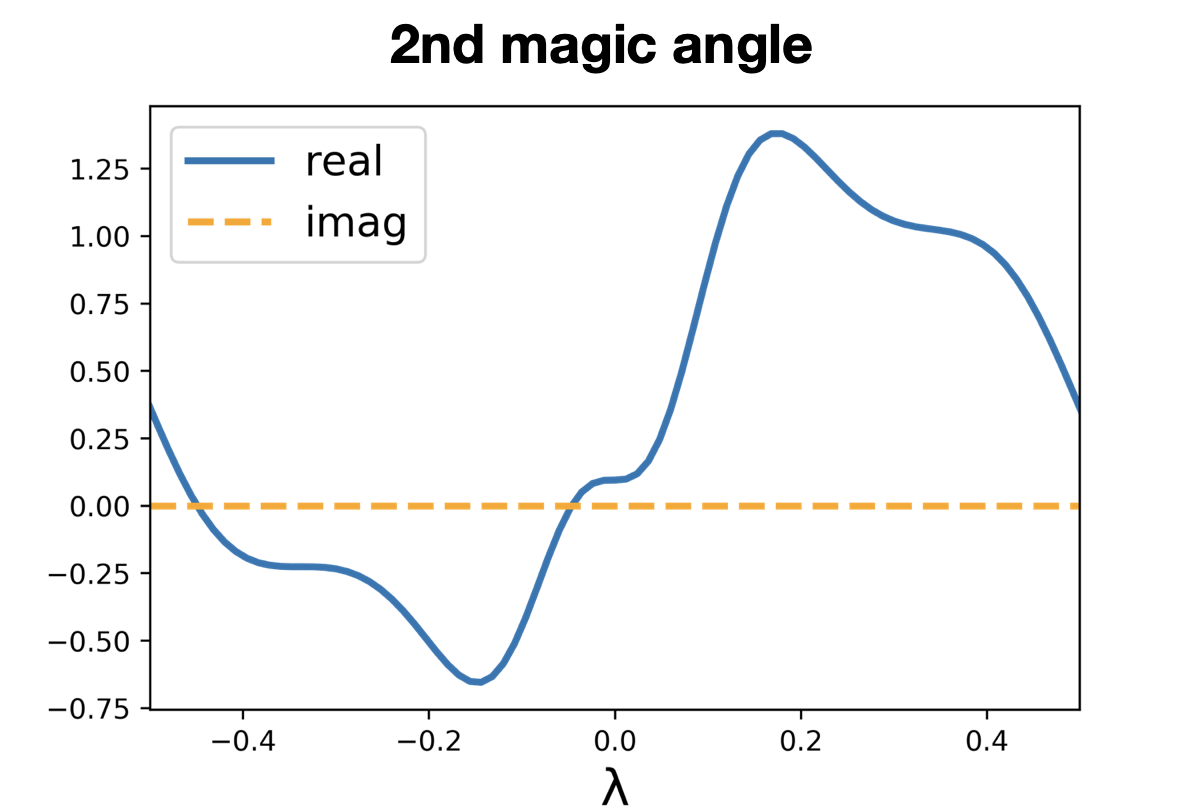

The zeros of the zero mode wavefunctions are classified into two types by their “movability”. One of them is a “movable zero” Arovas et al. 1988; Kohmoto 1985; Czerwinski and Brown 1991 from the quantum Hall wavefunction , whose location moves linearly with the Bloch wavevector:
| (40) |
This zero carries the external Hall response of the Chern band. There are other “frozen zeros” whose locations are fixed and independent of the Bloch momentum . In particular, among these frozen zeros, one of them is from the anti-quantum Hall state. In FIG. 5, we illustrate the zero-structure, where the black and blue dot represent the movable quantum Hall zero and the frozen anti-quantum Hall zeros. The yellow and red dots are frozen zeros from the function .
Besides their “movability”, zeros are also classified by their “chirality”: the wavefunction receives a phase when the coordinate encircles the zero once anticlockwise. We numerically noticed that the black and red dots are = zeros, while yellow and blue are = zeros. Interestingly, as shown in FIG. 1 the center of the unit cells are concentrated with more and more = zeros at higher magic angles. We discuss the implication for circulating currents in the next section.

We have shown that the zero mode wavefunction shares some similarities with the simple harmonic oscillator system whose eigenstates also have alternating parity and have an increasing number of zeros. In Appendix D, we provide an analytical argument why these features might persist for all higher magic angles by an analogy to the harmonic oscillator Swanson.
VI Experimental Observation and Implications
VI.1 Charge density and scanning tunneling probes
One direct consequence of the zeros is a charge density deficiency that can be seen in scanning tunneling spectroscopy experiments Jiang et al. 2019; Isobe et al. 2018; Guinea and Walet 2018.
We expect a spectroscopy experiment will probe only the top (or bottom) layer, which corresponds to the components (top layer sublattice wavefunction) and (top layer sublattice wavefunction). If the spectroscopy measurement has spatial resolution on the level of the atomic spacing, then the sublattice wavefunctions can be probed separately. In this case, fixed zeros in the wavefunction components or correspond to the vanishing of charge density in real space, which will be strongly visible in the spectroscopy experiment. If the ground state is sublattice polarized, which maybe the case on a hexagonal boron nitride substrate, then such spatial resolution is not required to observe the zeros in a spectroscopy experiment. Notice that since the opposite valley wavefunction on the same sublattice is related by , which acts trivially in real space, we expect the two opposite valley wavefunctions on the same sublattice have the same location of fixed zeros. Therefore, probing the zeros with spectroscopy does not require valley polarization.
The accumulation of zeros at the unit cell center and the unit cell boundary as magic angle order increases, as shown in FIG. 1, should also be visible by spectroscopy with even less atomic resolution. This accumulation will become more prominent at higher magic angles.
Away from the chiral model, the zeros become non-zero minima in the charge density, which we have observed numerically. These will give a less sharp signature in scanning tunneling spectroscopy experiments, but will likely still be observable over some parameter regime.
VI.2 Higher Landau level physics at higher magic angles
As we have seen from Section V, the piece of the flatband wavefunction in Eqn. (1) has an increasing number of zeros and has an analytical expansion similar to an anti-quantum Hall wavefunction. Consequently, we interpreted the zero mode wavefunction as a product of a higher Landau level anti-quantum Hall state and a lowest Landau level quantum Hall state (Eqn. (37)), where the Landau level index of the former is determined by the order of the magic angle. We also discussed in Section V.2 that the topological properties of the flatbands are determined by the lowest Landau level quantum Hall piece since does not have Bloch momentum dependence.
Nevertheless, we expect the effective interactions projected into the flatbands are modified strongly by both and . In particular, the nodal structure of directly impacts the charge density, which determines the projected Coulomb interaction. In the quantum Hall problem, the nodal structure of the higher Landau levels results in arrangement of charge that ultimately stabilizes various states Koulakov et al. 1996; Rezayi and Haldane 2000; Yang et al. 2001; Wan and Yang 2016 such as charge density waves, bubble phases, and other many-body topological phases (for instance, the non-Abelian Moore-Read phase Moore and Read 1991) that are absent in the lowest Landau level. By analogy, we might expect a different set of interacting phases to be stabilized at higher magic angles than at the first magic angle. Our formulation provides a theoretical and computational pathway towards analyzing interacting physics at different magic angles.
VI.3 Local current and magnetization at higher magic angles
From the charge density of the zero mode wavefunction as plotted in FIG. 1, we observe that for the first magic angle, the charge density maximum occurs at the unit cell center, i.e. the AA stacking point. At higher magic angles, we see an increasing number of zeros appearing at this region. Interestingly, all these zeros are of the same chirality for both layers, while zeros of the opposite chirality are pushed to the boundary of the unit cell. This indicates a stronger phase winding effect and hence circulating currents near the AA stacking region at higher magic angles, which could be experimentally observable nearby the chiral limit.
To see the circulation currents, we first define the following intra-sublattice intra-layer “current operator” for sublattice and layer . The operator is defined as:
| (41) |
operator is defined in a similar manner but with replaced by . Here is the microscopic parameter representing the next-nearest-neighbor hopping strength. We call the above a “current operator” in quot because is not the current operator of the chiral model, which by definition should be proportional to , and hence couples distinct sublattices and vanishes within one sublattice. Since the exact flatband wavefunctions are fully sublattice polarized (corresponding physically to hexagonal boron nitride splitting the sublattice degeneracy), the current operator vanishes within one sublattice polarized state. Nevertheless, we argue that our current operator has a microscopic origin, and hence should be a physical current operator. The can be regarded as a continuum version of lattice current induced from the next-nearest-neighbor hopping process in graphene, where the are graphene’s electron annihilation operators and labels graphene’s next-nearest-neighbor sites.

In FIG. 6, we plot the real space distribution of , calculated from the bottom layer sublattice- wavefunction at three different Bloch momenta. According to Ref. (He et al. 2020), the orbital magnetization is dominated by the Gamma point and Dirac point in a single valley model, since the bands hybridize most strongly with other bands at these points. Given the strong circulating current present at the second magic angle, it is reasonable to speculate a stronger orbital magnetization Thonhauser et al. 2005; Ceresoli et al. 2006; Sai et al. 2002; Xiao et al. 2005; Shi et al. 2007; Xiao et al. 2010; THONHAUSER 2011 at higher magic angles than the magnetization at the first magic angle Liu et al. 2019b; He et al. 2020; Li et al. 2019 for cases close to the chiral limit. Note that the circulation currents are odd under time reversal or a sublattice transformation, hence a strong experimental signal requires valley and sublattice polarization. We leave a detailed exploration of higher magic angle orbital magnetization with more realistic parameters as future work.
VII Conclusion
In this work, we studied the chiral model of twisted bilayer graphene introduced in Ref. (Tarnopolsky et al. 2019). We pointed out the intrinsic intra-valley inversion symmetry of the chiral model, protected by the crystal symmetry and the linearized Dirac fermion. As a consequence, the energy spectrum is inversion symmetric at all twist angles. Furthermore, zero modes occurring at different magic angles are distinguished by their intra-valley inversion eigenvalue. We numerically found a correspondence of the zero mode inversion parity and the order of magic angles and speculated such an alternating pattern would hold for all magic angles.
We also pointed out the intricate relation between the zero mode wavefunction and the quantum Hall wavefunctions. As guaranteed by intra-valley inversion symmetry, the zero mode wavefunction has an internal spinor structure, and in fact each component can be regarded as a product of a quantum Hall and an anti-quantum Hall wavefunction, which guarantees the zero mode has the periodicity of a Bloch wavefunction. Interestingly, there are an increasing number of zeros occurring in each component at higher magic angles.
In the end, we discussed the implications of our results to realistic systems and observable phenomena. First, these zeros can be detected as charge minima in real space by scanning tunneling spectroscopy. Second, the increasing number of zeros present in the zero mode wavefunction resembles the increasing number of zeros present in higher Landau level wavefunctions. Motivated by this observation, we anticipate higher Landau level physics will occur at the second and higher magic angles. Moreover, we noticed the phase circulation of the flatband wavefunctions at higher magic angles, and anticipate phenomena related to magnetization. We leave more detailed studies on higher magic angles as future work. We notice an earlier work on low twist angle physics in Ref. (Shi et al. 2020).
Last but not least, it is well known that on a compact manifold, a magnetic field is subject to a Dirac quantization condition Aharonov and Casher 1979. Our identification of zero mode wavefunctions with two quantum Hall wavefunctions may also shed light on the non-Abelian quantization condition San-Jose et al. 2012; Pacholski et al. 2018; Kailasvuori 2009, where a semi-classical analysis was done recently in Ref. (Ren et al. 2020).
Note added: during the final stage of the manuscript, we noticed the “unitary particle-hole” symmetry occurring in Ref. (Song et al. 2020) which is similar but distinct from our intra-valley inversion symmetry in Eqn. (15); we contrast the difference between the two in the paragraphs under Eqn. (18). We also noticed a relevant work on the chiral model, Ref. (Popov and Milekhin 2020), that appeared recently.
Acknowledgments
The Flatiron Institute is a division of the Simons Foundation. This work was partially supported by the Air Force Office of Scientific Research under Grant No. FA9550-20-1-0260 (J.C.).
Appendices
Appendix A Model Hamiltonians and Unitary Transformations
A.1 Lattices
We start with setting up the notation of moiré lattice. As mentioned in the main text, we denote the two dimensional lattice vectors as . The area of unit cell is defined to be :
| (42) |
where ==1 is the anti-symmetric symbol. The reciprocal basis vectors are:
| (43) |
As will be shown in Appendix C, defines an effective magnetic length. We set = throughout this work.
Graphene contains and sites. As shown in FIG. 2 of the main text, the Dirac points and sites are located at,
| (44) |
We use for throughout this work.
A.2 Unitary transformations
In Section II, we described the Bistritzer-MacDonald Hamiltonian Eqn. (3) and the chiral model Eqn. (8) of a single valley. They are written in the non-chiral and the chiral basis respectively, see Eqn. (4) and Eqn. (9). In this section, following Ref. (Tarnopolsky et al. 2019), we work out the details of the unitary transformation between the two bases. We start with the continuum model Eqn. (3), and perform a gauge transformation to remove the momentum shift on the diagonal. The Hamiltonian is transformed to be:
| (45) |
where is given in Eqn. (6). Then, we remove the diagonal dependence by rotation:
| (46) |
where
| (47) |
The matrix is the chiral Hamiltonian organized in basis where and represent the and sublattice respectively, and represent the bottom and top layer components. More explicitly,
| (48) |
where is defined in Eqn. (13). Transforming into the chiral basis Eqn. (9), we obtain Eqn. (8):
| (49) | |||||
The unitary transformation Eqn. (10) can be easily worked out from matrices , and the basis shuffling. As defined in the main text, we denote the rotated graphene Dirac points as , and denote the moiré Dirac points as =, = where is the moiré Brillouin zone center. We have also shifted the Bloch momentum of the chiral basis Eqn. (9) to center at the moiré Gamma point. Its Bloch translation symmetry can be also worked out easily as shown in Eqn. (11).
Appendix B How Symmetry Constrains the Chiral Hamiltonian
We have written the inter-layer coupling matrix in real space as Eqn. (3). We now discuss the action of , which complex conjugates and exchanges the two sublattices. The diagonal blocks in Eqn. (3) are invariant under this transformation. We now consider the off-diagonal tunneling terms . Its transformation under reads,
where, same as the main text, the Pauli matrices act on sublattice space. By virtue of being invariant under , it follows that:
| (50) |
or, element by element:
| (51) |
If we rotate to the chiral basis Eqn. (9), the tunneling terms enter in the following way:
| (52) |
where the diagonal blocks are:
| (53) |
and the off-diagonal blocks are:
| (54) |
Using the action of in Eqn. (51), these can be written in terms of only one complex parameter :
| (55) |
which satisfy our Lemma 1:
| (56) |
where the Pauli matrices act on the layer index.
In this basis, the chiral matrix that anti-commutes with the Hamiltonian enforces ==. Notice that Eqn. (56) also requires linearized Dirac fermion; a quadratic term in the dispersion destroys it. Note that a quadratic term in the dispersion also destroys the exact flatband of the chiral model. We hence demonstrated that for chiral models with linearized Dirac fermion, intra-valley inversion follows from symmetry.
Appendix C Quantum Hall Wavefunction
In this section we review the quantum Hall wavefunction that is frequently used in the main text. We start with discussing magnetic translation symmetry and quasi-periodic elliptic functions.
C.1 Magnetic translation symmetry
Since the lowest Landau level wavefunctions are usually written in terms of holomorphic functions, we start by setting up a notation for complex coordinates. Complex structures and define a one-to-one mapping from two dimensional affine space to the complex plane. We represent the metric and the anti-symmetric tensor as
| (57) |
They have the properties: , , and . The complex vectors are defined by contracting complex structure with vectors , and complex co-vectors as . To distinguish with vectors, complex vectors are unbold. In terms of complex coordinates, the inner product and cross product are respectively =+, =. In this work, we took and .
The quantum Hall system describes two dimensional interacting or noninteracting electrons in a perpendicular magnetic field. In a magnetic field, the electron’s coordinate is factorized into the center of its cyclotron motion i.e. guiding center , and the radius i.e. Landau orbits :
| (58) |
where commutes with , but their individual components are noncommutative:
| (59) |
In our case the area of unit cell plays the same role as magnetic length squared = where are electron charge and magnetic field strength. When projected into a single Landau level, an electron is fully described by the noncommutative degrees of freedom. The magnetic translation operator is defined as the following one,
| (60) |
which translates the guiding center by distance . The magnetic translation algebra is,
Due to the single value of wavefunction, any legal wavefunction must transform back to itself after a periodic translation. So we have the boundary condition,
| (61) |
where is a lattice vector. From now on we define the whole lattice as . The phase factor effectively measures the fraction of flux inside the torus. The wavefunctions that satisfy Eqn. (61) are written in terms of elliptic functions. One choice of elliptic function is the Jacobi theta function Haldane and Rezayi 1985. Recently it was also found that the “modified Weierstrass sigma function” is another choice Haldane 2018; Wang et al. 2019. Compared with Jacobi theta function, Weierstrass sigma function has the advantage of being modular invariant.
C.2 Modified Weierstrass sigma function
The modified Weierstrass sigma function Haldane 2018; Wang et al. 2019 is defined as:
| (62) |
i.e. a product of the standard Weierstrass sigma function and a holomorphic factor , where as will be explained soon the “almost modular form” is a modular independent number constant that vanishes for square and hexagonal torus. We now introduce the , and discuss the quasi-periodic property of .
The standard Weierstrass sigma function has a product series expansion (which is also a fast converging form for numerics),
| (63) |
where as defined above, means the set of lattice points. Clearly, it is modular invariant. It is also quasi-periodic,
where is the standard zeta function evaluated at half period, which is related to the =1 Eisenstein series , ,
| (64) |
The Eisenstein series has a highly convergent formula,
| (65) |
The in addition obey a relation that defines chirality,
| (66) |
In our case, the magnetic flux quanta of a unit cell is one, so =1. The (64) and (66) suggests a modular independent quantity called “almost modular form”,
| (67) |
With these formulas in hand, we are ready to get the quasi-periodicity of :
| (68) |
Last but not least, the sigma function is odd under spatial inversion: .
C.3 Quantum Hall wavefunction
The quantum Hall wavefunction is given in Eqn. (31), which we copy below:
It has a single zero located at = in each unit cell, with defined in Eqn. (24). Mapping to the complex plane, the zero occurs at and its translated counterparts, where is:
| (69) |
where the first term is zero following from Eqn. (43) and Eqn. (44). We used Eqn. (57) to derive the second term.
Since is not a Bloch function, the “Bloch vector” here should be understood as labeling the magnetic translation boundary condition Eqn. (61): =. For a quantum Hall wavefunction, its zero moves linearly with the boundary condition , reflecting the fact of Chern number = Arovas et al. 1988. The following diagram FIG. 7 is helpful to quickly figure out given the Bloch momentum .

Using results derived in the last section, it is easy to find the quasi-periodic boundary condition satisfies in real and reciprocal space. With =1,2, they are:
| (70) | |||||
| (71) |
The nontrivial phase factors above cannot be removed by a smooth, global, gauge transformation, which reflects the fact that has a nontrivial Chern number. Technically, these boundary conditions allow one to restrict the discussion to the unit cell and the first Brillouin zone. From now on, we denote as Bloch momentum inside the first Brillouin zone.
It is straightforward to see how inversion acts on quantum Hall wavefunctions from Eqn. (69):
| (72) |
Appendix D Analytical Argument for the Nodal Structure
The alternating parities and the increasing number of zeros we observed in the chiral model shares many similarities as the simple harmonic oscillator. In this section, we provide an argument for the zero-structure and inversion patterns by making an analogy to simple one-dimensional harmonic oscillators. Specifically, since the additional zeros that occur at higher magic angles occur along a reflection symmetric line, we reduce the zero mode equation to a one variable ordinary differential equation on that line. We can then compare to a harmonic oscillator in one dimension.
The one-dimensional harmonic oscillator is described by the Hamiltonian:
| (74) |
whose eigenstate satisfies the eigen-equation:
| (75) |
which can be transformed into the standard Sturm-Liouville form, with dimensionless parameters , and :
| (76) |
where
| (77) |
The normalizable solutions of Eqn. (76) are given by,
| (78) |
where = is the normalization factor and is the Hermite polynomial. Therefore we see that for the harmonic oscillator, the number of zeros of the -th excited eigenstate is , and the parity of the eigenstate alternates as . Such oscillatory behavior is a generic feature for Sturm-Liouville type differential equations Eqn. (76) on the interval where and are positive Swanson.
We have observed a similar alternating parity and increasing number of zeros of eigenstates at higher magic angles in the chiral model, as discussed in Section III.2 and Section V.3. The problem of the chiral twisted bilayer graphene model is more difficult. One reason is that it is a two-variable differential equation. To make progress, we utilize the symmetry of the problem to reduce the problem to one variable.
We starting by reviewing the zero mode equation, and see how symmetry helps reduce the dimension of the problem. We first recall the zero mode equation from Eqn. (1) and Eqn. (12):
| (79) |
By using the lowest Landau level condition that the quantum Hall wavefunction satisfies,
| (80) |
we arrive at the zero mode equation that the function must satisfy:
| (81) |
which is subject to the boundary condition Eqn. (73).
We note that due to the mirror symmetry of the problem, both and are zero mode solutions of Eqn. (81). By utilizing the global phase degree of freedom of wavefunction, one can always choose to be a purely real number, thereby constraining to be a real function. We have already used this property for in Section V.3, and plotted its real and imaginary part on the reflection symmetric line in FIG. 4.
Here we denote the real and imaginary parts of as and respectively. Although the imaginary part vanishes identically at =, its direction derivative does not. We end up with the following:
| (82) |
The zero mode equation Eqn. (81) is now rewritten as:
| (83) |
subject to the boundary condition Eqn. (73) which, when reduced to the = line, becomes:
| (84) | |||||
where is the length of the moiré primitive lattice vectors. In the unit = we have been using, its value is =.
The derivation so far is exact. The differential equation Eqn. (83) and its boundary conditions Eqn. (84) contain the full information of the nodes in the problem. The difficulty of solving Eqn. (83) is that it is a two-variable differential equation. To make progress, we now do approximation on to eliminate one variable.
It is interesting to observe that satisfies the same boundary condition as . In the following, we will approximate:
| (85) |
Under this assumption, the differential equation simplifies dramatically, and becomes a one-variable ordinary differential equation:
| (86) |
which can be rewritten into a second order form:
| (87) |
Hence we have brought the zero mode equation on the reflection symmetric line into the Sturm-Liouville form Eqn. (76) under the approximation shown in Eqn. (85).
Suppose we have two solutions of Eqn. (87), which corresponds to two magic angles with . From Eqn. (87), we deduce that,
where we have implicitly suppressed the argument in , and their derivatives. Now, consider a region spanned . The integration of the above equation in this region yields:
| (88) |
It then follows from the theory of differential equations Swanson, in the parameter region that or , the nodes of two consecutive solutions must oscillate; otherwise it leads to contradiction with Eqn. (88). We emphasize that our argument is based on the assumption Eqn. (85), and we can only argue for the node oscillation in the regions where are both positive or negative. This argument shows that in general, there should be more zeros at higher magic angles.
References
- Bistritzer and MacDonald (2011) Rafi Bistritzer and Allan H. MacDonald, “Moiré bands in twisted double-layer graphene,” Proceedings of the National Academy of Sciences 108, 12233–12237 (2011), https://www.pnas.org/content/108/30/12233.full.pdf .
- Lopes dos Santos et al. (2012) J. M. B. Lopes dos Santos, N. M. R. Peres, and A. H. Castro Neto, “Continuum model of the twisted graphene bilayer,” Phys. Rev. B 86, 155449 (2012).
- Lopes dos Santos et al. (2007) J. M. B. Lopes dos Santos, N. M. R. Peres, and A. H. Castro Neto, “Graphene bilayer with a twist: Electronic structure,” Phys. Rev. Lett. 99, 256802 (2007).
- Mele (2010) E. J. Mele, “Commensuration and interlayer coherence in twisted bilayer graphene,” Phys. Rev. B 81, 161405 (2010).
- Cao et al. (2018a) Yuan Cao, Valla Fatemi, Shiang Fang, Kenji Watanabe, Takashi Taniguchi, Efthimios Kaxiras, and Pablo Jarillo-Herrero, “Unconventional superconductivity in magic-angle graphene superlattices,” Nature 556, 43–50 (2018a).
- Cao et al. (2018b) Yuan Cao, Valla Fatemi, Ahmet Demir, Shiang Fang, Spencer L. Tomarken, Jason Y. Luo, Javier D. Sanchez-Yamagishi, Kenji Watanabe, Takashi Taniguchi, Efthimios Kaxiras, Ray C. Ashoori, and Pablo Jarillo-Herrero, “Correlated insulator behaviour at half-filling in magic-angle graphene superlattices,” Nature 556, 80–84 (2018b).
- Serlin et al. (2020) M. Serlin, C. L. Tschirhart, H. Polshyn, Y. Zhang, J. Zhu, K. Watanabe, T. Taniguchi, L. Balents, and A. F. Young, “Intrinsic quantized anomalous hall effect in a moiré heterostructure,” Science 367, 900–903 (2020).
- Sharpe et al. (2019) Aaron L. Sharpe, Eli J. Fox, Arthur W. Barnard, Joe Finney, Kenji Watanabe, Takashi Taniguchi, M. A. Kastner, and David Goldhaber-Gordon, “Emergent ferromagnetism near three-quarters filling in twisted bilayer graphene,” Science 365, 605–608 (2019).
- Yankowitz et al. (2019) Matthew Yankowitz, Shaowen Chen, Hryhoriy Polshyn, Yuxuan Zhang, K. Watanabe, T. Taniguchi, David Graf, Andrea F. Young, and Cory R. Dean, “Tuning superconductivity in twisted bilayer graphene,” Science 363, 1059–1064 (2019).
- Polshyn et al. (2019) Hryhoriy Polshyn, Matthew Yankowitz, Shaowen Chen, Yuxuan Zhang, K. Watanabe, T. Taniguchi, Cory R. Dean, and Andrea F. Young, “Large linear-in-temperature resistivity in twisted bilayer graphene,” Nature Physics 15, 1011–1016 (2019).
- Saito et al. (2020) Yu Saito, Jingyuan Ge, Kenji Watanabe, Takashi Taniguchi, and Andrea F. Young, “Independent superconductors and correlated insulators in twisted bilayer graphene,” Nature Physics (2020), 10.1038/s41567-020-0928-3.
- Tang et al. (2020) Yanhao Tang, Lizhong Li, Tingxin Li, Yang Xu, Song Liu, Katayun Barmak, Kenji Watanabe, Takashi Taniguchi, Allan H. MacDonald, Jie Shan, and Kin Fai Mak, “Simulation of hubbard model physics in wse2/ws2 moirésuperlattices,” Nature 579, 353–358 (2020).
- Balents et al. (2020) Leon Balents, Cory R. Dean, Dmitri K. Efetov, and Andrea F. Young, “Superconductivity and strong correlations in moiréflat bands,” Nature Physics 16, 725–733 (2020).
- Xu and Balents (2018) Cenke Xu and Leon Balents, “Topological superconductivity in twisted multilayer graphene,” Phys. Rev. Lett. 121, 087001 (2018).
- Wu et al. (2018) Fengcheng Wu, A. H. MacDonald, and Ivar Martin, “Theory of phonon-mediated superconductivity in twisted bilayer graphene,” Phys. Rev. Lett. 121, 257001 (2018).
- Lian et al. (2019) Biao Lian, Zhijun Wang, and B. Andrei Bernevig, “Twisted bilayer graphene: A phonon-driven superconductor,” Phys. Rev. Lett. 122, 257002 (2019).
- Hu et al. (2019) Xiang Hu, Timo Hyart, Dmitry I. Pikulin, and Enrico Rossi, “Geometric and conventional contribution to the superfluid weight in twisted bilayer graphene,” Phys. Rev. Lett. 123, 237002 (2019).
- Xie et al. (2020a) Fang Xie, Zhida Song, Biao Lian, and B. Andrei Bernevig, “Topology-bounded superfluid weight in twisted bilayer graphene,” Phys. Rev. Lett. 124, 167002 (2020a).
- Wu and Das Sarma (2020) Fengcheng Wu and Sankar Das Sarma, “Collective excitations of quantum anomalous hall ferromagnets in twisted bilayer graphene,” Phys. Rev. Lett. 124, 046403 (2020).
- Zhang et al. (2019) Ya-Hui Zhang, Dan Mao, Yuan Cao, Pablo Jarillo-Herrero, and T. Senthil, “Nearly flat chern bands in moiré superlattices,” Phys. Rev. B 99, 075127 (2019).
- Gao et al. (2020) Yang Gao, Yinhan Zhang, and Di Xiao, “Tunable layer circular photogalvanic effect in twisted bilayers,” Phys. Rev. Lett. 124, 077401 (2020).
- Li et al. (2010) Guohong Li, A. Luican, J. M. B. Lopes dos Santos, A. H. Castro Neto, A. Reina, J. Kong, and E. Y. Andrei, “Observation of van hove singularities in twisted graphene layers,” Nature Physics 6, 109–113 (2010).
- Trambly de Laissardière et al. (2010) G. Trambly de Laissardière, D. Mayou, and L. Magaud, “Localization of dirac electrons in rotated graphene bilayers,” Nano Letters, Nano Letters 10, 804–808 (2010).
- Rademaker and Mellado (2018) Louk Rademaker and Paula Mellado, “Charge-transfer insulation in twisted bilayer graphene,” Phys. Rev. B 98, 235158 (2018).
- Xie and MacDonald (2020) Ming Xie and A. H. MacDonald, “Nature of the correlated insulator states in twisted bilayer graphene,” Phys. Rev. Lett. 124, 097601 (2020).
- González and Stauber (2020) J. González and T. Stauber, “Marginal fermi liquid in twisted bilayer graphene,” Phys. Rev. Lett. 124, 186801 (2020).
- Saito et al. (2020) Yu Saito, Jingyuan Ge, Kenji Watanabe, Takashi Taniguchi, Erez Berg, and Andrea F. Young, “Isospin Pomeranchuk effect and the entropy of collective excitations in twisted bilayer graphene,” arXiv e-prints , arXiv:2008.10830 (2020), arXiv:2008.10830 [cond-mat.mes-hall] .
- Lu et al. (2020) Xiaobo Lu, Biao Lian, Gaurav Chaudhary, Benjamin A. Piot, Giulio Romagnoli, Kenji Watanabe, Takashi Taniguchi, Martino Poggio, Allan H. MacDonald, B. Andrei Bernevig, and Dmitri K. Efetov, “Fingerprints of Fragile Topology in the Hofstadter spectrum of Twisted Bilayer Graphene Close to the Second Magic Angle,” arXiv e-prints , arXiv:2006.13963 (2020), arXiv:2006.13963 [cond-mat.mes-hall] .
- Khalaf et al. (2020) Eslam Khalaf, Nick Bultinck, Ashvin Vishwanath, and Michael P. Zaletel, “Soft modes in magic angle twisted bilayer graphene,” (2020), arXiv:2009.14827 [cond-mat.str-el] .
- Mele (2011) E. J. Mele, “Band symmetries and singularities in twisted multilayer graphene,” Phys. Rev. B 84, 235439 (2011).
- Po et al. (2018) Hoi Chun Po, Liujun Zou, Ashvin Vishwanath, and T. Senthil, “Origin of mott insulating behavior and superconductivity in twisted bilayer graphene,” Phys. Rev. X 8, 031089 (2018).
- Zou et al. (2018) Liujun Zou, Hoi Chun Po, Ashvin Vishwanath, and T. Senthil, “Band structure of twisted bilayer graphene: Emergent symmetries, commensurate approximants, and wannier obstructions,” Phys. Rev. B 98, 085435 (2018).
- Kang and Vafek (2018) Jian Kang and Oskar Vafek, “Symmetry, maximally localized wannier states, and a low-energy model for twisted bilayer graphene narrow bands,” Phys. Rev. X 8, 031088 (2018).
- Koshino et al. (2018) Mikito Koshino, Noah F. Q. Yuan, Takashi Koretsune, Masayuki Ochi, Kazuhiko Kuroki, and Liang Fu, “Maximally localized wannier orbitals and the extended hubbard model for twisted bilayer graphene,” Phys. Rev. X 8, 031087 (2018).
- Song et al. (2019) Zhida Song, Zhijun Wang, Wujun Shi, Gang Li, Chen Fang, and B. Andrei Bernevig, “All magic angles in twisted bilayer graphene are topological,” Phys. Rev. Lett. 123, 036401 (2019).
- Isobe et al. (2018) Hiroki Isobe, Noah F. Q. Yuan, and Liang Fu, “Unconventional superconductivity and density waves in twisted bilayer graphene,” Phys. Rev. X 8, 041041 (2018).
- Po et al. (2019) Hoi Chun Po, Liujun Zou, T. Senthil, and Ashvin Vishwanath, “Faithful tight-binding models and fragile topology of magic-angle bilayer graphene,” Phys. Rev. B 99, 195455 (2019).
- Carr et al. (2019) Stephen Carr, Shiang Fang, Hoi Chun Po, Ashvin Vishwanath, and Efthimios Kaxiras, “Derivation of wannier orbitals and minimal-basis tight-binding hamiltonians for twisted bilayer graphene: First-principles approach,” Phys. Rev. Research 1, 033072 (2019).
- Vafek and Kang (2020) Oskar Vafek and Jian Kang, “Towards the hidden symmetry in Coulomb interacting twisted bilayer graphene: renormalization group approach,” arXiv e-prints , arXiv:2009.09413 (2020), arXiv:2009.09413 [cond-mat.str-el] .
- Kang and Vafek (2019) Jian Kang and Oskar Vafek, “Strong coupling phases of partially filled twisted bilayer graphene narrow bands,” Phys. Rev. Lett. 122, 246401 (2019).
- Bultinck et al. (2020a) Nick Bultinck, Eslam Khalaf, Shang Liu, Shubhayu Chatterjee, Ashvin Vishwanath, and Michael P. Zaletel, “Ground state and hidden symmetry of magic-angle graphene at even integer filling,” Phys. Rev. X 10, 031034 (2020a).
- Bernevig et al. (2020) B. Andrei Bernevig, Zhida Song, Nicolas Regnault, and Biao Lian, “TBG I: Matrix Elements, Approximations, Perturbation Theory and a 2-Band Model for Twisted Bilayer Graphene,” arXiv e-prints , arXiv:2009.11301 (2020), arXiv:2009.11301 [cond-mat.mes-hall] .
- Song et al. (2020) Zhi-Da Song, Biao Lian, Nicolas Regnault, and Andrei B. Bernevig, “Tbg ii: Stable symmetry anomaly in twisted bilayer graphene,” (2020), arXiv:2009.11872 [cond-mat.mes-hall] .
- Bernevig et al. (2020a) B. Andrei Bernevig, Zhida Song, Nicolas Regnault, and Biao Lian, “Tbg iii: Interacting hamiltonian and exact symmetries of twisted bilayer graphene,” (2020a), arXiv:2009.12376 [cond-mat.str-el] .
- Lian et al. (2020) Biao Lian, Zhi-Da Song, Nicolas Regnault, Dmitri K. Efetov, Ali Yazdani, and B. Andrei Bernevig, “Tbg iv: Exact insulator ground states and phase diagram of twisted bilayer graphene,” (2020), arXiv:2009.13530 [cond-mat.str-el] .
- Bernevig et al. (2020b) B. Andrei Bernevig, Biao Lian, Aditya Cowsik, Fang Xie, Nicolas Regnault, and Zhi-Da Song, “Tbg v: Exact analytic many-body excitations in twisted bilayer graphene coulomb hamiltonians: Charge gap, goldstone modes and absence of cooper pairing,” (2020b), arXiv:2009.14200 [cond-mat.str-el] .
- Xie et al. (2020b) Fang Xie, Aditya Cowsik, Zhida Son, Biao Lian, B. Andrei Bernevig, and Nicolas Regnault, “Tbg vi: An exact diagonalization study of twisted bilayer graphene at non-zero integer fillings,” (2020b), arXiv:2010.00588 [cond-mat.str-el] .
- Bultinck et al. (2020b) Nick Bultinck, Shubhayu Chatterjee, and Michael P. Zaletel, “Mechanism for anomalous hall ferromagnetism in twisted bilayer graphene,” Phys. Rev. Lett. 124, 166601 (2020b).
- Abouelkomsan et al. (2020) Ahmed Abouelkomsan, Zhao Liu, and Emil J. Bergholtz, “Particle-hole duality, emergent fermi liquids, and fractional chern insulators in moiré flatbands,” Phys. Rev. Lett. 124, 106803 (2020).
- Repellin et al. (2020) Cécile Repellin, Zhihuan Dong, Ya-Hui Zhang, and T. Senthil, “Ferromagnetism in narrow bands of moiré superlattices,” Phys. Rev. Lett. 124, 187601 (2020).
- Repellin and Senthil (2020) Cécile Repellin and T. Senthil, “Chern bands of twisted bilayer graphene: Fractional Chern insulators and spin phase transition,” Physical Review Research 2, 023238 (2020), arXiv:1912.11469 [cond-mat.str-el] .
- Tarnopolsky et al. (2019) Grigory Tarnopolsky, Alex Jura Kruchkov, and Ashvin Vishwanath, “Origin of magic angles in twisted bilayer graphene,” Phys. Rev. Lett. 122, 106405 (2019).
- Liu et al. (2019a) Jianpeng Liu, Junwei Liu, and Xi Dai, “Pseudo landau level representation of twisted bilayer graphene: Band topology and implications on the correlated insulating phase,” Phys. Rev. B 99, 155415 (2019a).
- Becker et al. (2020) Simon Becker, Mark Embree, Jens Wittsten, and Maciej Zworski, “Mathematics of magic angles in a model of twisted bilayer graphene,” (2020), arXiv:2008.08489 [math-ph] .
- Ledwith et al. (2020) Patrick J. Ledwith, Grigory Tarnopolsky, Eslam Khalaf, and Ashvin Vishwanath, “Fractional chern insulator states in twisted bilayer graphene: An analytical approach,” Phys. Rev. Research 2, 023237 (2020).
- Haldane (2018) F. D. M. Haldane, “A modular-invariant modified weierstrass sigma-function as a building block for lowest-landau-level wavefunctions on the torus,” Journal of Mathematical Physics 59, 071901 (2018), https://doi.org/10.1063/1.5042618 .
- Wang et al. (2019) Jie Wang, Scott D. Geraedts, E. H. Rezayi, and F. D. M. Haldane, “Lattice monte carlo for quantum hall states on a torus,” Phys. Rev. B 99, 125123 (2019).
- Geraedts et al. (2018) Scott D. Geraedts, Jie Wang, E. H. Rezayi, and F. D. M. Haldane, “Berry phase and model wave function in the half-filled landau level,” Phys. Rev. Lett. 121, 147202 (2018).
- Wang (2019) Jie Wang, “Dirac fermion hierarchy of composite fermi liquids,” Phys. Rev. Lett. 122, 257203 (2019).
- Haldane and Rezayi (1985) F. D. M. Haldane and E. H. Rezayi, “Periodic laughlin-jastrow wave functions for the fractional quantized hall effect,” Phys. Rev. B. 31, 2529 (1985).
- Laughlin (1981) R. B. Laughlin, “Quantized hall conductivity in two dimensions,” Phys. Rev. B 23, 5632–5633 (1981).
- Arovas et al. (1988) Daniel P. Arovas, R. N. Bhatt, F. D. M. Haldane, P. B. Littlewood, and R. Rammal, “Localization, wave-function topology, and the integer quantized hall effect,” Phys. Rev. Lett. 60, 619–622 (1988).
- Kohmoto (1985) Mahito Kohmoto, “Topological invariant and the quantization of the hall conductance,” Annals of Physics 160, 343 – 354 (1985).
- Czerwinski and Brown (1991) M. Czerwinski and E. Brown, “A nodal determination of the hall conductance,” Proceedings: Mathematical and Physical Sciences 433, 547–571 (1991).
- (65) C. A. Swanson, Comparison and Oscillation Theory of Linear Differential Equations, edited by Richard Bellman (Elsevier).
- Jiang et al. (2019) Yuhang Jiang, Xinyuan Lai, Kenji Watanabe, Takashi Taniguchi, Kristjan Haule, Jinhai Mao, and Eva Y. Andrei, “Charge order and broken rotational symmetry in magic-angle twisted bilayer graphene,” Nature 573, 91–95 (2019).
- Guinea and Walet (2018) Francisco Guinea and Niels R. Walet, “Electrostatic effects, band distortions, and superconductivity in twisted graphene bilayers,” Proceedings of the National Academy of Sciences 115, 13174–13179 (2018), https://www.pnas.org/content/115/52/13174.full.pdf .
- Koulakov et al. (1996) A. A. Koulakov, M. M. Fogler, and B. I. Shklovskii, “Charge density wave in two-dimensional electron liquid in weak magnetic field,” Phys. Rev. Lett. 76, 499–502 (1996).
- Rezayi and Haldane (2000) E. H. Rezayi and F. D. M. Haldane, “Incompressible paired hall state, stripe order, and the composite fermion liquid phase in half-filled landau levels,” Phys. Rev. Lett. 84, 4685–4688 (2000).
- Yang et al. (2001) Kun Yang, F. D. M. Haldane, and E. H. Rezayi, “Wigner crystals in the lowest landau level at low-filling factors,” Phys. Rev. B 64, 081301 (2001).
- Wan and Yang (2016) Xin Wan and Kun Yang, “Striped quantum hall state in a half-filled landau level,” Phys. Rev. B 93, 201303 (2016).
- Moore and Read (1991) Gregory Moore and Nicholas Read, “Nonabelions in the fractional quantum hall effect,” Nuclear Physics B 360, 362 (1991).
- He et al. (2020) Wen-Yu He, David Goldhaber-Gordon, and K. T. Law, “Giant orbital magnetoelectric effect and current-induced magnetization switching in twisted bilayer graphene,” Nature Communications 11, 1650 (2020).
- Thonhauser et al. (2005) T. Thonhauser, Davide Ceresoli, David Vanderbilt, and R. Resta, “Orbital magnetization in periodic insulators,” Phys. Rev. Lett. 95, 137205 (2005).
- Ceresoli et al. (2006) Davide Ceresoli, T. Thonhauser, David Vanderbilt, and R. Resta, “Orbital magnetization in crystalline solids: Multi-band insulators, chern insulators, and metals,” Phys. Rev. B 74, 024408 (2006).
- Sai et al. (2002) Na Sai, Karin M. Rabe, and David Vanderbilt, “Theory of structural response to macroscopic electric fields in ferroelectric systems,” Phys. Rev. B 66, 104108 (2002).
- Xiao et al. (2005) Di Xiao, Junren Shi, and Qian Niu, “Berry phase correction to electron density of states in solids,” Phys. Rev. Lett. 95, 137204 (2005).
- Shi et al. (2007) Junren Shi, G. Vignale, Di Xiao, and Qian Niu, “Quantum theory of orbital magnetization and its generalization to interacting systems,” Phys. Rev. Lett. 99, 197202 (2007).
- Xiao et al. (2010) Di Xiao, Ming-Che Chang, and Qian Niu, “Berry phase effects on electronic properties,” Rev. Mod. Phys. 82, 1959–2007 (2010).
- THONHAUSER (2011) T. THONHAUSER, “Theory of orbital magnetization in solids,” International Journal of Modern Physics B 25, 1429–1458 (2011), https://doi.org/10.1142/S0217979211058912 .
- Liu et al. (2019b) Jianpeng Liu, Zhen Ma, Jinhua Gao, and Xi Dai, “Quantum valley hall effect, orbital magnetism, and anomalous hall effect in twisted multilayer graphene systems,” Phys. Rev. X 9, 031021 (2019b).
- Li et al. (2019) Si-Yu Li, Yu Zhang, Ya-Ning Ren, Jianpeng Liu, Xi Dai, and Lin He, “Experimental evidence for orbital magnetic moments generated by moiré-scale current loops in twisted bilayer graphene,” arXiv e-prints , arXiv:1912.13133 (2019), arXiv:1912.13133 [cond-mat.mtrl-sci] .
- Shi et al. (2020) Haohao Shi, Zhen Zhan, Zhikai Qi, Kaixiang Huang, Edo van Veen, Jose Ángel Silva-Guillén, Runxiao Zhang, Pengju Li, Kun Xie, Hengxing Ji, Mikhail I. Katsnelson, Shengjun Yuan, Shengyong Qin, and Zhenyu Zhang, “Large-area, periodic, and tunable intrinsic pseudo-magnetic fields in low-angle twisted bilayer graphene,” Nature Communications 11, 371 (2020).
- Aharonov and Casher (1979) Y. Aharonov and A. Casher, “Ground state of a spin-1/2 charged particle in a two-dimensional magnetic field,” Phys. Rev. A 19, 2461–2462 (1979).
- San-Jose et al. (2012) P. San-Jose, J. González, and F. Guinea, “Non-abelian gauge potentials in graphene bilayers,” Phys. Rev. Lett. 108, 216802 (2012).
- Pacholski et al. (2018) M. J. Pacholski, C. W. J. Beenakker, and İ. Adagideli, “Topologically protected landau level in the vortex lattice of a weyl superconductor,” Phys. Rev. Lett. 121, 037701 (2018).
- Kailasvuori (2009) J. Kailasvuori, “Pedestrian index theorem à la aharonov-casher for bulk threshold modes in corrugated multilayer graphene,” EPL (Europhysics Letters) 87, 47008 (2009).
- Ren et al. (2020) Yafei Ren, Qiang Gao, A. H. MacDonald, and Qian Niu, “WKB estimate of bilayer graphene’s magic twist angles,” arXiv e-prints , arXiv:2006.13292 (2020), arXiv:2006.13292 [cond-mat.mes-hall] .
- Popov and Milekhin (2020) Fedor K. Popov and Alexey Milekhin, “Hidden wave function of twisted bilayer graphene: Flat band as a landau level,” (2020), arXiv:2010.02915 [cond-mat.str-el] .