Quantum simulation of open quantum systems in heavy-ion collisionsPreprint: MIT-CTP/5247

Wibe A. de Jong Email: wadejong@lbl.gov Affiliation: Computational Research Division, Lawrence Berkeley National Laboratory, Berkeley, CA 94720, USA Mekena Metcalf Email: mmetcalf@lbl.gov Affiliation: Computational Research Division, Lawrence Berkeley National Laboratory, Berkeley, CA 94720, USA James Mulligan Email: james.mulligan@berkeley.edu Affiliation: Nuclear Science Division, Lawrence Berkeley National Laboratory, Berkeley, California 94720, USA Affiliation: Physics Department, University of California, Berkeley, CA 94720, USA Mateusz Płoskoń Email: mploskon@lbl.gov Affiliation: Nuclear Science Division, Lawrence Berkeley National Laboratory, Berkeley, California 94720, USA Felix Ringer Email: fmringer@lbl.gov Affiliation: Nuclear Science Division, Lawrence Berkeley National Laboratory, Berkeley, California 94720, USA Xiaojun Yao Email: xjyao@mit.edu Affiliation: Center for Theoretical Physics, Massachusetts Institute of Technology, Cambridge, MA 02139, USA

August 11, 2026

Abstract

We present a framework to simulate the dynamics of hard probes such as heavy quarks or jets in a hot, strongly-coupled quark-gluon plasma (QGP) on a quantum computer. Hard probes in the QGP can be treated as open quantum systems governed in the Markovian limit by the Lindblad equation. However, due to large computational costs, most current phenomenological calculations of hard probes evolving in the QGP use semiclassical approximations of the quantum evolution. Quantum computation can mitigate these costs, and offers the potential for a fully quantum treatment with exponential speedup over classical techniques. We report a simplified demonstration of our framework on IBM Q quantum devices, and apply the Random Identity Insertion Method (RIIM) to account for cnot depolarization noise, in addition to measurement error mitigation. Our work demonstrates the feasibility of simulating open quantum systems on current and near-term quantum devices, which is of broad relevance to applications in nuclear physics, quantum information, and other fields.

Introduction. Considerable advancements in quantum devices, such as qubit coherence times, have recently been achieved Devoret2013; annurev-conmatphys-031119-050605; doi:10.1063/1.5088164; google_supremacy. Together with parallel progress in quantum algorithms and executable quantum software, nontrivial quantum computations can be carried out, including hybrid quantum-classical algorithms such as the variational quantum eigensolver McClean_2016; Peruzzo_2014; Kandala2017; Rubin2020; PhysRevX.8.011021; Chong2017 and fully quantum simulations of the unitary time evolution of closed quantum systems PhysRevB.101.184305; Smith2019. In high energy and nuclear physics, a variety of quantum computing applications have emerged Preskill_2018; Jordan:2011ne; Kaplan:2017ccd; Preskill:2018fag; Klco:2018zqz; Dumitrescu:2018njn; Klco:2018kyo; Chang:2018uoc; Roggero:2019myu; Klco:2019evd; Roggero:2019srp; Cloet:2019wre; Bauer:2019qxa; Mueller:2019qqj; Wei:2019rqy; Holland:2019zju; Avkhadiev:2019niu; Shaw:2020udc; Liu:2020eoa; Kreshchuk:2020dla; Kharzeev:2020kgc; Klco:2020aud; DiMatteo:2020dhe; Davoudi:2020yln; Bepari:2020xqi. In particular, quantum simulation can be applied to study dynamics of large size systems that are in principle intractable with classical methods. To perform such simulations, quantum circuits compiled into single- and multi-qubit gates can be implemented on digital quantum computers.

Many physical systems of interest are not closed, but consist of a subsystem interacting with an environment. The dynamics of the subsystem can be formulated as an open quantum system. In the Markovian limit (in which the environment correlation time is much smaller than the subsystem relaxation time), the evolution of the subsystem is governed by a generalization of the Schrödinger equation known as the Lindblad equation KOSSAKOWSKI1972247; Lindblad:1975ef; Gorini:1976cm, where instead of keeping track of all of the environmental degrees of freedom, one only needs to record environment correlators that are relevant for the subsystem evolution. A key challenge in extending quantum simulation to open quantum systems is that the Lindblad evolution is non-unitary. During the last decade, algorithms have been developed to overcome this issue, most of which couple the subsystem with auxiliary qubits (whose dimension can be significantly smaller than that of the environment) such that the whole system evolves unitarily PhysRevA.83.062317; PhysRevA.91.062308; Wei:2016; cleve_et_al:LIPIcs:2017:7477; PhysRevLett.118.140403; PhysRevA.101.012328; PhysRevResearch.2.023214. More recently, simulations of open quantum systems have been carried out on real quantum devices, but without error mitigation Hu:2019.

In this letter, we focus on the application of quantum simulations of open quantum systems to relativistic heavy-ion collisions (HICs). Experiments at the Relativistic Heavy Ion Collider (RHIC) and the Large Hadron Collider (LHC) create a hot ( $T\approx 150-500$ MeV), short-lived ( $t\approx 10\;\mathrm{fm}/c$ ) quark-gluon plasma (QGP) PhysRevD.27.140; Arsene:2004fa; Adcox:2004mh; Back:2004je; Adams:2005dq; LHC1review; Braun-Munzinger:2015hba; TheBigPicture. The QGP is a deconfined phase of QCD matter believed to have existed shortly after the Big Bang Weinberg:1977ji. The properties of the QGP can be investigated using jets or heavy quarks Adare:2010de; Sirunyan:2017isk; Adamczyk:2017yhe; Acharya:2019jyg; Aaboud:2018twu that involve energy scales much larger than the QGP temperature (“hard probes”).

The evolution of hard probes in the QGP can be treated as an open system evolving in a hot medium. A fully field-theoretical description of hard probes in the medium is challenging and typically various approximations are made. Most studies employ semiclassical Boltzmann or Fokker-Planck (equivalent to Langevin) equations Gossiaux:2008jv; Schenke:2009gb; Wang:2013cia; Cao:2016gvr; Cao:2015hia; Du:2017qkv; Ke:2018tsh; Yao:2020xzw; semiclassical transport equations are leading order terms in the gradient expansion of the Wigner transformed Lindblad equation Blaizot:2017ypk; Yao:2020eqy. Recently, several studies have applied Lindblad equations directly to investigate quarkonia Young:2010jq; Akamatsu:2011se; Gossiaux:2016htk; Brambilla:2017zei; Yao:2018nmy; Miura:2019ssi; Sharma:2019xum; Brambilla:2020qwo and jets Vaidya:2020cyi; Vaidya:2020lih, which are valid if the subsystem and environment are weakly coupled. It is expected that as the size of the subsystem increases (such as the jet radiation phase space, or the number of heavy quarks Andronic:2007bi; Abada:2019lih in the subsystem), solving Lindblad equations would challenge the limits of classical computation. Quantum computing offers a possibility to remove the constraint on the subsystem size, and go beyond the approximations made in semiclassical approaches. Moreover, quantum simulation may provide a solution to the notoriously difficult sign problem in classical lattice QCD calculations of real time observables Jordan:2011ne; Jordan:2011ci; Martinez_2016; Haase:2020kaj (the same problem can also appear in open QCD systems).

In this letter, we outline a formulation of the evolution of hard probes in the QGP as a Lindblad equation and explore how simulations on Noisy Intermediate Scale Quantum (NISQ Preskill_2018) devices can be used to advance theoretical studies of hard probes in the QGP. Using a quantum algorithm for simulating the Lindblad equation, we study a toy model on IBM Q simulators and quantum devices, and implement error mitigation for measurement and two-qubit gate noise. We demonstrate that quantum algorithms simulating simple Lindblad evolution are tractable on current and near-term devices, in terms of available number of qubits, gate depth, and error rates.

Open quantum system formulation of hard probes in heavy-ion collisions. The Hamiltonian of the full system consisting of the hard probe (subsystem) and the QGP (environment) can be written as

	$\displaystyle H$	$\displaystyle=$	$\displaystyle H_{S}+H_{E}+H_{I}$		(1)
	$\displaystyle H_{S}$	$\displaystyle=$	$\displaystyle H_{S0}+H_{S1}\,.$		(2)

Here $H_{S}$ , $H_{E}$ and $H_{I}$ are the Hamiltonians of the subsystem, the environment and their interaction, respectively. A schematic diagram of the setup is shown in Fig. 1. We further split $H_{S}$ into the free $H_{S0}$ and the interacting part of the subsystem $H_{S1}$ . In quantum field theories, Hamiltonians are functionals of fields, which require discretization in position space Preskill:2018fag. Here, instead of simulating the dynamics of fields, we focus on simulating the dynamics of particle states, which is valid for hard probes. If we use multi-particle states $|p_{1},A_{1}\rangle\otimes\cdots\otimes|p_{n},A_{n}\rangle$ as the basis where $p_{i}$ is the four-momentum, $A_{i}$ represents all discrete quantum numbers, and $i=1,2,\ldots,n$ , then both $H_{S0}$ and $H_{S1}$ are matrices and $H_{S0}$ is diagonal. Note that $H_{S1}$ is different from $H_{I}$ : The former is the interaction within the subsystem itself and independent of the environment, while the latter represents the interaction between the subsystem and the environment. For example, for jets in HICs, $H_{S1}$ can be collinear radiation of collinear particles while $H_{I}$ can describe the Glauber exchange between collinear particles (subsystem) and soft fields from the QGP environment Vaidya:2020cyi.

Refer to caption — Figure 1: A schematic illustration of a multi-level open quantum system $S$ interacting with a thermal environment $E$ . The levels in $S$ can represent for example: (1) heavy quark-antiquark ( $Q\bar{Q}$ ) bound states $|{\boldsymbol{p}},A_{i}\rangle$ with center-of-mass momentum ${\boldsymbol{p}}$ and quantum numbers $A_{i}$ , and (2) unbound $Q\bar{Q}$ pairs $|{\boldsymbol{p}}_{1},{\boldsymbol{p}}_{2}\rangle$ with momenta ${\boldsymbol{p}}_{1},{\boldsymbol{p}}_{2}$ . For jets the levels of $S$ can represent multi-parton states labeled by momenta $|p_{1},\cdots,p_{n}\rangle$ .

The total density matrix of the subsystem and the environment evolves under the von Neumann equation. In the interaction picture, this is given by

\displaystyle\frac{\mathop{}\!\mathrm{d}}{\mathop{}\!\mathrm{d}t}\rho^{(\mathrm{int})}(t)=-i[H^{(\mathrm{int})}_{I}(t),\rho^{(\mathrm{int})}(t)]\,.

(3)

The operators are defined by

$\displaystyle\rho^{(\mathrm{int})}(t)$	$\displaystyle\equiv$	$\displaystyle e^{i(H_{S0}+H_{E})t}\rho(t)e^{-i(H_{S0}+H_{E})t}$	(4)
$\displaystyle H_{S1}^{(\mathrm{int})}(t)$	$\displaystyle\equiv$	$\displaystyle e^{iH_{S0}t}H_{S1}e^{-iH_{S0}t}$	(5)
$\displaystyle H_{I}^{(\mathrm{int})}(t)$	$\displaystyle\equiv$	$\displaystyle e^{i(H_{S0}+H_{E})t}H_{I}e^{-i(H_{S0}+H_{E})t}\,.$	(6)

The interaction picture used here is special: it is the standard interaction picture for the subsystem but it is the Heisenberg picture for the environment. We will drop the superscript (int) from now on for simplicity but the reader should be reminded that we use the interaction picture throughout. We assume that the initial density matrix factorizes and the environment density matrix is a thermal state¹¹ 1 The backreaction of the QGP medium to jet energy loss CasalderreySolana:2004qm; Ruppert:2005uz; Chaudhuri:2005vc; Qin:2009uh; Betz:2010qh; Floerchinger:2014yqa; Chen:2017zte; Yan:2017rku; Tachibana:2020mtb; Casalderrey-Solana:2020rsj, which may further modify jet observables is beyond the scope of our considerations here. For a recent review, see Ref. Cao:2020wlm.

	$\displaystyle\rho(0)$	$\displaystyle=$	$\displaystyle\rho_{S}(0)\otimes\rho_{E}$		(7)
	$\displaystyle\rho_{E}$	$\displaystyle=$	$\displaystyle\frac{e^{-\beta H_{E}}}{\mathrm{Tr}(e^{-\beta H_{E}})}\,,$		(8)

where $\beta=1/T$ is the inverse of the QGP temperature.

After the environment is traced out, the reduced evolution of the subsystem density matrix is generally time-irreversible and non-unitary. If the coupling between the subsystem and the environment is weak, the reduced evolution equation can be cast as a Markovian Lindblad equation KOSSAKOWSKI1972247; Lindblad:1975ef; Gorini:1976cm:

	$\displaystyle\frac{\mathop{}\!\mathrm{d}}{\mathop{}\!\mathrm{d}t}\rho_{S}(t)=$	$\displaystyle-i\big[H_{S1}(t)+H_{L},\rho_{S}(t)\big]$
		$\displaystyle+\sum_{j=1}^{m}\Big(L_{j}\rho_{S}(t)L_{j}^{\dagger}-\frac{1}{2}\big\{L_{j}^{\dagger}L_{j},\rho_{S}(t)\big\}\Big)\,,$		(9)

where $H_{L}$ denotes a thermal correction to $H_{S}$ generated by loop effects of $H_{I}$ , and the $L_{j}$ are called Lindblad operators, whose explicit expressions will be given for a toy model below. In general, if the dimension of the subsystem is $d$ , (i.e., $\rho_{S}(t)$ is a $d\times d$ matrix), the number of independent Lindblad operators is $m=d^{2}-1$ . When evaluating the Lindblad operators, an environment correlator of the form $\mathrm{Tr}_{E}[O_{E}(t_{1})O_{E}(t_{2})\rho_{E}]$ is needed as input, where the $O_{E}$ ’s are some environment operators. This correlator can be evaluated perturbatively in thermal field theory if the environment is weakly-coupled. But the construction of the Lindblad equation only requires $H_{I}$ to be weak. In general $H_{E}$ itself can be strongly coupled, in which case the correlator has to be computed nonperturbatively using lattice QCD Petreczky:2005nh; Banerjee:2011ra; Majumder:2012sh; Francis:2015daa; Brambilla:2020siz or the AdS/CFT correspondence Liu:2006ug; Liu:2006he; CasalderreySolana:2006rq; CaronHuot:2008uh; CasalderreySolana:2011us. For the nonperturbative computation, one needs to formulate the theory such that the relevant correlator is gauge invariant, where effective field theory can be used. A concrete construction of gauge invariant correlators for quarkonium transport can be found in Refs. Yao:2020eqy; Brambilla:2019tpt.

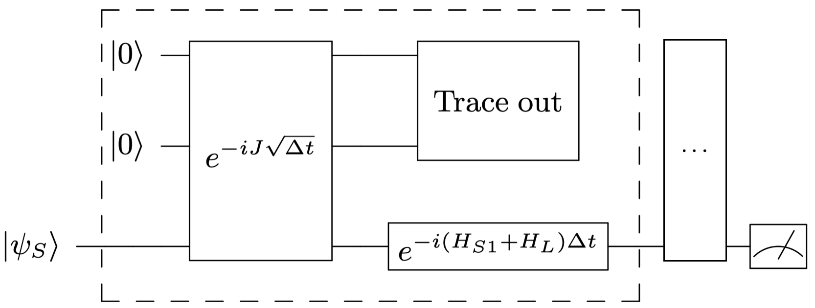
Quantum algorithm. We will apply a quantum algorithm based on the Stinespring dilation theorem, see for example Refs. nielsen_chuang_2010; cleve_et_al:LIPIcs:2017:7477, to simulate the Lindblad equation. The algorithm in terms of the evolution operators $J$ , defined below, and $H_{S}$ , is illustrated in Fig. 2. The algorithm couples the subsystem with auxiliary qubits, which are traced out after each time step $\Delta t$ . The dimension of the auxiliary register is $m+1$ and the number of qubits needed in practice for the register is $\mathrm{ceil}(\log_{2}(m+1))\equiv\lceil{2\log_{2}d}\rceil$ . Together with the number of qubits required to record the subsystem state, the total number of qubits needed is $\lceil{3\log_{2}d}\rceil$ . We use $\{|0\rangle_{a},|1\rangle_{a}\cdots,|m\rangle_{a}\}$ to label the basis of the auxiliary register, indicated by the subscript $a$ .

We assume the initial state $\rho_{S}(0)=|\psi_{S}(0)\rangle\langle\psi_{S}(0)|$ is a pure state²² 2 If it is a mixed state, then we decompose it into a linear superposition of pure states. We just need to apply the circuit to each pure state and take the linear superposition in the end.. At the beginning of each cycle at time $t$ , the total density matrix of the subsystem and the auxiliary is set to be a $(m+1)\times(m+1)$ block matrix

\displaystyle\rho(t)=|0\rangle_{a}\langle 0|_{a}\otimes\rho_{S}(t)=\begin{pmatrix}\rho_{S}(t)&0&\dots&0\\ 0&0&\dots&0\\ \vdots&\vdots&\ddots&\vdots\\ 0&0&\dots&0\end{pmatrix}\,.

(10)

The $J$ -operator is also a $(m+1)\times(m+1)$ block matrix

\displaystyle J=\begin{pmatrix}0&L_{1}^{\dagger}&\dots&L_{m}^{\dagger}\\ L_{1}&0&\dots&0\\ \vdots&\vdots&\ddots&\vdots\\ L_{m}&0&\dots&0\end{pmatrix}\,,

(11)

where each block is a $d\times d$ matrix. One can show that the circuit in Fig. 2 reproduces (Quantum simulation of open quantum systems in heavy-ion collisions) when $\Delta t\to 0$ . To simulate the evolution from $0$ to $t$ , the size of the time steps is $\Delta t=t/N_{\mathrm{cycle}}$ where $N_{\mathrm{cycle}}$ is the number of cycles, see Fig. 2.

Toy model and simulation on IBM Q. Simulating real jets and heavy quarks on quantum devices requires a large number of fault-tolerant qubits. As a proof of concept, we consider the following toy model that includes qualitative features of hard probes:

$\displaystyle H_{S}$	$\displaystyle=\,H_{S0}=-\frac{\Delta E}{2}Z$	(12)
$\displaystyle H_{E}$	$\displaystyle=\,\int\mathop{}\!\mathrm{d}^{3}x\bigg[\frac{1}{2}\Pi^{2}+\frac{1}{2}(\nabla\phi)^{2}+\frac{1}{2}m^{2}\phi^{2}+\frac{1}{4!}\lambda\phi^{4}\bigg]$	(13)
$\displaystyle H_{I}$	$\displaystyle=\,gX\otimes\phi(x=0)\,,$	(14)

where we use $X,Z$ to denote the single qubit Pauli gates (Pauli matrices). The subsystem Hamiltonian $H_{S}$ is a two level system with energy difference $\Delta E$ . The two levels can correspond to the bound and unbound state of a heavy quark-antiquark pair, exchanging energy with QGP. The environment $H_{E}$ is a $3+1D$ scalar field theory, that together with (8) mimics the thermal QGP. Here $\Pi$ is the canonical momentum conjugate to $\phi$ . The extension to gauge theories requires a gauge invariant formulation of the environment correlator as mentioned earlier. The environment correlator can be calculated nonperturbatively to all orders in $\lambda$ . Here for simplicity, we set $m=\lambda=0$ . Nonvanishing $m$ and $\lambda$ lead to different coefficients of the Lindblad operators but do not alter the quantum algorithm. The interaction strength $g$ between the subsystem and the environment is unitless. In the Markovian limit, two Lindblad operators $j=0,1$ are relevant:

L_{j}=\frac{\sqrt{\Gamma_{j}}}{2}(X-(-1)^{j}iY)\,,

(15)

where $\Gamma_{0}=g^{2}\Delta En_{B}(\Delta E)/(2\pi)$ , $\Gamma_{1}=g^{2}\Delta E/(2\pi)+\Gamma_{0}$ and $n_{B}(\Delta E)=1/(\exp(\beta\Delta E)-1)$ is the Bose-Einstein distribution. We will neglect $H_{L}$ in this letter. For our numerical studies, we use a unit system where all quantities are counted in units of $T$ , the temperature of the medium. We initialize the state as $\rho_{S}(t=0)=|0\rangle\langle 0|$ and choose $\Delta E=1(T)$ .

Figure 3: Simulation of the quantum circuit with

N_{\rm{cycle}}=100

for various system-environment couplings, along with numerical solution using a 4th order Runge-Kutta method. The upper time axis corresponds to a medium with a temperature of

T=300

MeV. Each time point in the simulator result consists of 80192 shots (runs).

The result for this toy model obtained from the IBM Q qiskit simulator Qiskit is shown in Fig. 3. We measure $P_{0}(t)\equiv\langle 0|\rho_{S}(t)|0\rangle$ , which can be interpreted as the time-dependent nuclear modification factor. Each time point corresponds to an independent quantum circuit, where the measurement is performed only at the end, as shown in Fig. 2. The results of the quantum algorithm with $N_{\rm{cycle}}{}=100$ are shown for different values of the coupling $g$ . They are consistent with the results obtained with a 4th order Runge-Kutta method that solves Eq. (Quantum simulation of open quantum systems in heavy-ion collisions) classically. This agreement demonstrates that the circuit successfully solves the Lindblad equation. As expected, the strength of the coupling $g$ controls the rate of approaching thermalization.

In order to run the circuit on a quantum device, we select $N_{\rm{cycle}}{}=1$ in order to achieve a sufficiently small circuit depth. Modern quantum software packages are available to compile quantum circuits that approximate general unitary operators with minimal error and optimal depth Chong2017; younis2020qfast; davis2019heuristics; qsearch_placeholder. We synthesize a circuit for the $e^{-iJ\sqrt{\Delta t}}$ operator in terms of single qubit and cnot gates using the qsearch compiler qsearch_placeholder. The compiler yields circuits with 70 gates on average, including approximately 10 cnots per cycle; an example circuit for one cycle is shown in the supplemental material.

Figure 4: Results from the IBM Q Vigo device including different error mitigations compared to results from the qiskit simulator for

N_{\rm cycle}=1

and

N_{\rm cycle}=3

and the Runge-Kutta method. Higher values of

N_{\rm cycle}

quickly converge to the result using the Runge-Kutta method. Each time point in the simulator result consists of 800192 shots (runs).

The results obtained from IBM Q Vigo device IBMQVigo are shown in Fig. 4. In addition to the uncorrected result, the results with readout and cnot error mitigation are also shown. We correct the readout error using the constrained matrix inversion approach in IBM’s qiskit-ignis package. The response matrix can be found in the supplemental material. We also correct for cnot noise using a leading order zero-noise extrapolation based on the recently developed resource efficient Random Identity Insertion Method (RIIM) He:2020udd. This procedure corrects for depolarization noise using a set of additional (cnot)² identity insertions, at the expense of amplifying statistical noise. Each data point corresponds to 5 evenly spaced time points that are averaged together. Each time point is calculated from the average of 49152 shots (runs). We observe that the error mitigation is more important at small values of $t$ . Similar results were reproduced on the IBM Q Valencia and Santiago devices IBMQValencia; IBMQSantiago.

Overall, we observe good agreement of the results from the quantum device with the results from the simulator for $N_{\rm{cycle}}{}=1$ after the error mitigation is applied. The choice of $N_{\rm{cycle}}{}=1$ is seen to be a reasonable approximation for sufficiently small $t$ . Moreover, a modest increase to $N_{\rm{cycle}}{}=3$ , as shown by the simulator in Fig. 4, yields considerably improved convergence, which is promising for near-term applications. These results demonstrate that the simulation of open quantum system dynamics relevant for HICs should be feasible on current and near-term quantum devices.

Conclusions and Outlook. We performed simulations of open quantum systems using quantum devices from IBM Q. In particular, we focused on simulating the non-unitary evolution of a subsystem governed by the Lindblad equation. We demonstrated that digital quantum simulations with a few qubits and a circuit depth of $\sim 70$ gate operations with $\sim 10$ cnot gates are feasible on current quantum devices. We used the qsearch compiler to construct the quantum circuit, and implemented two-qubit gate error mitigation using zero noise extrapolation with the Random Identity Insertion Method (RIIM), in addition to readout error mitigation. Simulating open quantum systems is of great importance for theoretical studies of hard probes in heavy-ion collisions. The open quantum system formulation allows one to go beyond semiclassical transport calculations currently used in most phenomenological studies. Future calculations, using a time dependent environment density matrix may allow one to explore a broad range of physical models by varying medium properties such as the initial temperature, microscopic structure, or the probe-medium coupling. Open quantum systems are also relevant for various other systems in nuclear and high-energy physics such as studies of Cold Nuclear Matter effects at the future Electron-Ion Collider Accardi:2012qut, the resummation of large logarithms relevant for jet physics Dasgupta:2001sh; Banfi:2002hw; Nagy:2007ty; Neill:2015nya and studies of the Color Glass Condensate Armesto:2019mna; Li:2020bys.

Acknowledgements.

Acknowledgements. We thank Christian Bauer, Volker Koch, Ben Nachman, Long-Gang Pang, Krishna Rajagopal, Phiala Shanahan, Rishi Sharma, Ramona Vogt, Xin-Nian Wang and Feng Yuan for helpful discussions. We acknowledge use of IBM Q for this work. The views expressed are those of the authors and do not reflect the official policy or position of IBM or the IBM Q team. JM, MP are supported by the U.S. Department of Energy, Office of Science, Office of Nuclear Physics, under the contract DE-AC02-05CH11231. FR is supported by LDRD funding from Berkeley Lab provided by the U.S. Department of Energy under Contract No. DE-AC02-05CH11231. XY is supported by the U.S. Department of Energy, Office of Science, Office of Nuclear Physics under grant Contract Number DE-SC0011090. MM and WDJ were supported by the U.S. Department of Energy, Office of Science, Office of Advanced Scientific Computing Research Accelerated Research in Quantum Computing program under contract DE-AC02-05CH11231. This research used resources of the Oak Ridge Leadership Computing Facility, which is a User Facility supported by U.S. Department of Energy, Office of Science, under Contract No. DE-AC05-00OR22725.

References

(1) M. Devoret and R. Schoelkopf, “Superconducting circuits for quantum information: An outlook,” Science (New York, N.Y.) 339 (03, 2013) 1169–74.
(2) M. Kjaergaard, M. E. Schwartz, J. Braumüller, P. Krantz, J. I.-J. Wang, S. Gustavsson, and W. D. Oliver, “Superconducting qubits: Current state of play,” Annual Review of Condensed Matter Physics 11 no. 1, (2020) 369–395.
(3) C. D. Bruzewicz, J. Chiaverini, R. McConnell, and J. M. Sage, “Trapped-ion quantum computing: Progress and challenges,” Applied Physics Reviews 6 no. 2, (2019) 021314.
(4) F. Arute, K. Arya, R. Babbush, D. Bacon, J. C. Bardin, R. Barends, R. Biswas, S. Boixo, F. G. S. L. Brandao, and D. A. e. a. Buell, “Quantum supremacy using a programmable superconducting processor,” Nature 574 no. 7779, (2019) 505–510. https://doi.org/10.1038/s41586-019-1666-5.
(5) J. R. McClean, J. Romero, R. Babbush, and A. Aspuru-Guzik, “The theory of variational hybrid quantum-classical algorithms,” New Journal of Physics 18 no. 2, (Feb, 2016) 023023.
(6) A. Peruzzo, J. McClean, P. Shadbolt, M.-H. Yung, X.-Q. Zhou, P. J. Love, A. Aspuru-Guzik, and J. L. O’Brien, “A variational eigenvalue solver on a photonic quantum processor,” Nature Communications 5 no. 1, (Jul, 2014) .
(7) A. Kandala, A. Mezzacapo, K. Temme, M. Takita, M. Brink, J. M. Chow, and J. M. Gambetta, “Hardware-efficient variational quantum eigensolver for small molecules and quantum magnets,” Nature 549 no. 7671, (2017) 242–246. https://doi.org/10.1038/nature23879.
(8) Google AI Quantum and collaborators, “Hartree-fock on a superconducting qubit quantum computer,” Science 369 (08, 2020) 1084–1089.
(9) J. I. Colless, V. V. Ramasesh, D. Dahlen, M. S. Blok, M. E. Kimchi-Schwartz, J. R. McClean, J. Carter, W. A. de Jong, and I. Siddiqi, “Computation of molecular spectra on a quantum processor with an error-resilient algorithm,” Phys. Rev. X 8 (Feb, 2018) 011021. https://link.aps.org/doi/10.1103/PhysRevX.8.011021.
(10) F. T. Chong, D. Franklin, and M. Martonosi, “Programming languages and compiler design for realistic quantum hardware,” Nature 549 (09, 2017) 180–187.
(11) L. Bassman, K. Liu, A. Krishnamoorthy, T. Linker, Y. Geng, D. Shebib, S. Fukushima, F. Shimojo, R. K. Kalia, A. Nakano, and P. Vashishta, “Towards simulation of the dynamics of materials on quantum computers,” Phys. Rev. B 101 (May, 2020) 184305. https://link.aps.org/doi/10.1103/PhysRevB.101.184305.
(12) A. Smith, M. S. Kim, F. Pollmann, and J. Knolle, “Simulating quantum many-body dynamics on a current digital quantum computer,” npj Quantum Information 5 (11, 2019) 106.
(13) J. Preskill, “Quantum computing in the nisq era and beyond,” Quantum 2 (Aug, 2018) 79. http://dx.doi.org/10.22331/q-2018-08-06-79.
(14) S. P. Jordan, K. S. Lee, and J. Preskill, “Quantum Algorithms for Quantum Field Theories,” Science 336 (2012) 1130–1133, arXiv:1111.3633 [quant-ph].
(15) D. B. Kaplan, N. Klco, and A. Roggero, “Ground States via Spectral Combing on a Quantum Computer,” arXiv:1709.08250 [quant-ph].
(16) J. Preskill, “Simulating quantum field theory with a quantum computer,” PoS LATTICE2018 (2018) 024, arXiv:1811.10085 [hep-lat].
(17) N. Klco and M. J. Savage, “Digitization of scalar fields for quantum computing,” Phys. Rev. A 99 no. 5, (2019) 052335, arXiv:1808.10378 [quant-ph].
(18) E. Dumitrescu, A. McCaskey, G. Hagen, G. Jansen, T. Morris, T. Papenbrock, R. Pooser, D. Dean, and P. Lougovski, “Cloud Quantum Computing of an Atomic Nucleus,” Phys. Rev. Lett. 120 no. 21, (2018) 210501, arXiv:1801.03897 [quant-ph].
(19) N. Klco, E. Dumitrescu, A. McCaskey, T. Morris, R. Pooser, M. Sanz, E. Solano, P. Lougovski, and M. Savage, “Quantum-classical computation of Schwinger model dynamics using quantum computers,” Phys. Rev. A 98 no. 3, (2018) 032331, arXiv:1803.03326 [quant-ph].
(20) C. C. Chang, A. Gambhir, T. S. Humble, and S. Sota, “Quantum annealing for systems of polynomial equations,” Sci. Rep. 9 no. 1, (2019) 10258, arXiv:1812.06917 [quant-ph].
(21) A. Roggero, A. C. Li, J. Carlson, R. Gupta, and G. N. Perdue, “Quantum Computing for Neutrino-Nucleus Scattering,” Phys. Rev. D 101 no. 7, (2020) 074038, arXiv:1911.06368 [quant-ph].
(22) N. Klco, J. R. Stryker, and M. J. Savage, “SU(2) non-Abelian gauge field theory in one dimension on digital quantum computers,” Phys. Rev. D 101 no. 7, (2020) 074512, arXiv:1908.06935 [quant-ph].
(23) A. Roggero and A. Baroni, “Short-depth circuits for efficient expectation value estimation,” Phys. Rev. A 101 no. 2, (2020) 022328, arXiv:1905.08383 [quant-ph].
(24) I. C. Cloët et al., “Opportunities for Nuclear Physics & Quantum Information Science,” in Intersections between Nuclear Physics and Quantum Information, I. C. Cloët and M. R. Dietrich, eds. 3, 2019. arXiv:1903.05453 [nucl-th].
(25) C. W. Bauer, W. A. de Jong, B. Nachman, and D. Provasoli, “Quantum Algorithm for High Energy Physics Simulations,” Phys. Rev. Lett. 126 no. 6, (2021) 062001, arXiv:1904.03196 [hep-ph].
(26) N. Mueller, A. Tarasov, and R. Venugopalan, “Deeply inelastic scattering structure functions on a hybrid quantum computer,” Phys. Rev. D 102 no. 1, (2020) 016007, arXiv:1908.07051 [hep-th].
(27) A. Y. Wei, P. Naik, A. W. Harrow, and J. Thaler, “Quantum Algorithms for Jet Clustering,” Phys. Rev. D 101 no. 9, (2020) 094015, arXiv:1908.08949 [hep-ph].
(28) E. T. Holland, K. A. Wendt, K. Kravvaris, X. Wu, W. Erich Ormand, J. L. DuBois, S. Quaglioni, and F. Pederiva, “Optimal Control for the Quantum Simulation of Nuclear Dynamics,” Phys. Rev. A 101 no. 6, (2020) 062307, arXiv:1908.08222 [quant-ph].
(29) A. Avkhadiev, P. Shanahan, and R. Young, “Accelerating Lattice Quantum Field Theory Calculations via Interpolator Optimization Using Noisy Intermediate-Scale Quantum Computing,” Phys. Rev. Lett. 124 no. 8, (2020) 080501, arXiv:1908.04194 [hep-lat].
(30) A. F. Shaw, P. Lougovski, J. R. Stryker, and N. Wiebe, “Quantum Algorithms for Simulating the Lattice Schwinger Model,” Quantum 4 (2020) 306, arXiv:2002.11146 [quant-ph].
(31) J. Liu and Y. Xin, “Quantum simulation of quantum field theories as quantum chemistry,” JHEP 12 (2020) 011, arXiv:2004.13234 [hep-th].
(32) M. Kreshchuk, W. M. Kirby, G. Goldstein, H. Beauchemin, and P. J. Love, “Quantum Simulation of Quantum Field Theory in the Light-Front Formulation,” arXiv:2002.04016 [quant-ph].
(33) D. E. Kharzeev and Y. Kikuchi, “Real-time chiral dynamics from a digital quantum simulation,” Phys. Rev. Res. 2 no. 2, (2020) 023342, arXiv:2001.00698 [hep-ph].
(34) N. Klco and M. J. Savage, “Fixed-point quantum circuits for quantum field theories,” Phys. Rev. A 102 no. 5, (2020) 052422, arXiv:2002.02018 [quant-ph].
(35) O. Di Matteo, A. Mccoy, P. Gysbers, T. Miyagi, R. M. Woloshyn, and P. Navrátil, “Improving Hamiltonian encodings with the Gray code,” Phys. Rev. A 103 no. 4, (2021) 042405, arXiv:2008.05012 [quant-ph].
(36) Z. Davoudi, I. Raychowdhury, and A. Shaw, “Search for Efficient Formulations for Hamiltonian Simulation of non-Abelian Lattice Gauge Theories,” arXiv:2009.11802 [hep-lat].
(37) K. Bepari, S. Malik, M. Spannowsky, and S. Williams, “Towards a quantum computing algorithm for helicity amplitudes and parton showers,” Phys. Rev. D 103 no. 7, (2021) 076020, arXiv:2010.00046 [hep-ph].
(38) A. Kossakowski, “On quantum statistical mechanics of non-hamiltonian systems,” Reports on Mathematical Physics 3 no. 4, (1972) 247 – 274.
(39) G. Lindblad, “On the Generators of Quantum Dynamical Semigroups,” Commun. Math. Phys. 48 (1976) 119.
(40) V. Gorini, A. Frigerio, M. Verri, A. Kossakowski, and E. Sudarshan, “Properties of Quantum Markovian Master Equations,” Rept. Math. Phys. 13 (1978) 149.
(41) H. Wang, S. Ashhab, and F. Nori, “Quantum algorithm for simulating the dynamics of an open quantum system,” Phys. Rev. A 83 (Jun, 2011) 062317.
(42) R. Sweke, I. Sinayskiy, D. Bernard, and F. Petruccione, “Universal simulation of markovian open quantum systems,” Phys. Rev. A 91 (Jun, 2015) 062308.
(43) S.-J. Wei, D. Ruan, and G.-L. Long, “Duality quantum algorithm efficiently simulates open quantum systems,” Scientific Reports 6 no. 1, (2016) 30727.
(44) R. Cleve and C. Wang, “Efficient Quantum Algorithms for Simulating Lindblad Evolution,” in 44th International Colloquium on Automata, Languages, and Programming (ICALP 2017). arXiv:1612.09512 [quant-ph].
(45) A. Chenu, M. Beau, J. Cao, and A. del Campo, “Quantum simulation of generic many-body open system dynamics using classical noise,” Phys. Rev. Lett. 118 (Apr, 2017) 140403.
(46) H.-Y. Su and Y. Li, “Quantum algorithm for the simulation of open-system dynamics and thermalization,” Phys. Rev. A 101 (Jan, 2020) 012328.
(47) M. Metcalf, J. E. Moussa, W. A. de Jong, and M. Sarovar, “Engineered thermalization and cooling of quantum many-body systems,” Phys. Rev. Research 2 (May, 2020) 023214. https://link.aps.org/doi/10.1103/PhysRevResearch.2.023214.
(48) Z. Hu, R. Xia, and S. Kais, “A quantum algorithm for evolving open quantum dynamics on quantum computing devices,” Scientific Reports 10 no. 1, (2020) 3301.
(49) J. D. Bjorken, “Highly relativistic nucleus-nucleus collisions: The central rapidity region,” Phys. Rev. D 27 (Jan, 1983) 140–151.
(50) BRAHMS Collaboration, I. Arsene et al., “Quark gluon plasma and color glass condensate at RHIC? The Perspective from the BRAHMS experiment,” Nucl. Phys. A 757 (2005) 1–27, arXiv:nucl-ex/0410020.
(51) PHENIX Collaboration, K. Adcox et al., “Formation of dense partonic matter in relativistic nucleus-nucleus collisions at RHIC: Experimental evaluation by the PHENIX collaboration,” Nucl. Phys. A 757 (2005) 184–283, arXiv:nucl-ex/0410003.
(52) PHOBOS Collaboration, B. Back et al., “The PHOBOS perspective on discoveries at RHIC,” Nucl. Phys. A 757 (2005) 28–101, arXiv:nucl-ex/0410022.
(53) STAR Collaboration, J. Adams et al., “Experimental and theoretical challenges in the search for the quark gluon plasma: The STAR Collaboration’s critical assessment of the evidence from RHIC collisions,” Nucl. Phys. A 757 (2005) 102–183, arXiv:nucl-ex/0501009.
(54) B. Müller, J. Schukraft, and B. Wysłouch, “First Results from Pb+Pb Collisions at the LHC,” Annu. Rev. Nucl. Part. S. 62 no. 1, (2012) 361–386.
(55) P. Braun-Munzinger, V. Koch, T. Schäfer, and J. Stachel, “Properties of hot and dense matter from relativistic heavy ion collisions,” Phys. Rept. 621 (2016) 76–126.
(56) W. Busza, K. Rajagopal, and W. van der Schee, “Heavy Ion Collisions: The Big Picture, and the Big Questions,” Ann. Rev. Nucl. Part. Sci. 68 (2018) 339–376.
(57) S. Weinberg, The First Three Minutes. A Modern View of the Origin of the Universe. ISBN: 9780465024377, Bantam Books, 1977.
(58) PHENIX Collaboration, A. Adare et al., “Heavy Quark Production in $p+p$ and Energy Loss and Flow of Heavy Quarks in Au+Au Collisions at $\sqrt{s_{NN}}=200$ GeV,” Phys. Rev. C 84 (2011) 044905, arXiv:1005.1627 [nucl-ex].
(59) CMS Collaboration, A. M. Sirunyan et al., “Measurement of prompt and nonprompt charmonium suppression in PbPb collisions at 5.02 TeV,” Eur. Phys. J. C 78 no. 6, (2018) 509, arXiv:1712.08959 [nucl-ex].
(60) STAR Collaboration, L. Adamczyk et al., “Measurements of jet quenching with semi-inclusive hadron+jet distributions in Au+Au collisions at $\sqrt{s_{NN}}$ = 200 GeV,” Phys. Rev. C 96 no. 2, (2017) 024905, arXiv:1702.01108 [nucl-ex].
(61) ALICE Collaboration, S. Acharya et al., “Measurements of inclusive jet spectra in pp and central Pb-Pb collisions at $\sqrt{s_{\rm{NN}}}$ = 5.02 TeV,” Phys. Rev. C 101 no. 3, (2020) 034911, arXiv:1909.09718 [nucl-ex].
(62) ATLAS Collaboration, M. Aaboud et al., “Measurement of the nuclear modification factor for inclusive jets in Pb+Pb collisions at $\sqrt{s_{\mathrm{NN}}}=5.02$ TeV with the ATLAS detector,” Phys. Lett. B 790 (2019) 108–128, arXiv:1805.05635 [nucl-ex].
(63) P. Gossiaux and J. Aichelin, “Towards an understanding of the RHIC single electron data,” Phys. Rev. C 78 (2008) 014904, arXiv:0802.2525 [hep-ph].
(64) B. Schenke, C. Gale, and S. Jeon, “MARTINI: An Event generator for relativistic heavy-ion collisions,” Phys. Rev. C 80 (2009) 054913, arXiv:0909.2037 [hep-ph].
(65) X.-N. Wang and Y. Zhu, “Medium Modification of $\gamma$ -jets in High-energy Heavy-ion Collisions,” Phys. Rev. Lett. 111 no. 6, (2013) 062301, arXiv:1302.5874 [hep-ph].
(66) S. Cao, T. Luo, G.-Y. Qin, and X.-N. Wang, “Linearized Boltzmann transport model for jet propagation in the quark-gluon plasma: Heavy quark evolution,” Phys. Rev. C 94 no. 1, (2016) 014909, arXiv:1605.06447 [nucl-th].
(67) S. Cao, G.-Y. Qin, and S. A. Bass, “Energy loss, hadronization and hadronic interactions of heavy flavors in relativistic heavy-ion collisions,” Phys. Rev. C 92 no. 2, (2015) 024907, arXiv:1505.01413 [nucl-th].
(68) X. Du, R. Rapp, and M. He, “Color Screening and Regeneration of Bottomonia in High-Energy Heavy-Ion Collisions,” Phys. Rev. C 96 no. 5, (2017) 054901, arXiv:1706.08670 [hep-ph].
(69) W. Ke, Y. Xu, and S. A. Bass, “Linearized Boltzmann-Langevin model for heavy quark transport in hot and dense QCD matter,” Phys. Rev. C 98 no. 6, (2018) 064901, arXiv:1806.08848 [nucl-th].
(70) X. Yao, W. Ke, Y. Xu, S. A. Bass, and B. Müller, “Coupled Boltzmann Transport Equations of Heavy Quarks and Quarkonia in Quark-Gluon Plasma,” JHEP 01 (2021) 046, arXiv:2004.06746 [hep-ph].
(71) J.-P. Blaizot and M. A. Escobedo, “Quantum and classical dynamics of heavy quarks in a quark-gluon plasma,” JHEP 06 (2018) 034, arXiv:1711.10812 [hep-ph].
(72) X. Yao and T. Mehen, “Quarkonium Semiclassical Transport in Quark-Gluon Plasma: Factorization and Quantum Correction,” JHEP 02 (2021) 062, arXiv:2009.02408 [hep-ph].
(73) C. Young and K. Dusling, “Quarkonium above deconfinement as an open quantum system,” Phys. Rev. C 87 no. 6, (2013) 065206, arXiv:1001.0935 [nucl-th].
(74) Y. Akamatsu and A. Rothkopf, “Stochastic potential and quantum decoherence of heavy quarkonium in the quark-gluon plasma,” Phys. Rev. D 85 (2012) 105011, arXiv:1110.1203 [hep-ph].
(75) P. B. Gossiaux and R. Katz, “Upsilon suppression in the Schrödinger–Langevin approach,” Nucl. Phys. A 956 (2016) 737–740, arXiv:1601.01443 [hep-ph].
(76) N. Brambilla, M. A. Escobedo, J. Soto, and A. Vairo, “Heavy quarkonium suppression in a fireball,” Phys. Rev. D 97 no. 7, (2018) 074009, arXiv:1711.04515 [hep-ph].
(77) X. Yao and T. Mehen, “Quarkonium in-medium transport equation derived from first principles,” Phys. Rev. D 99 no. 9, (2019) 096028, arXiv:1811.07027 [hep-ph].
(78) T. Miura, Y. Akamatsu, M. Asakawa, and A. Rothkopf, “Quantum Brownian motion of a heavy quark pair in the quark-gluon plasma,” Phys. Rev. D 101 no. 3, (2020) 034011, arXiv:1908.06293 [nucl-th].
(79) R. Sharma and A. Tiwari, “Quantum evolution of quarkonia with correlated and uncorrelated noise,” Phys. Rev. D 101 no. 7, (2020) 074004, arXiv:1912.07036 [hep-ph].
(80) N. Brambilla, M. A. Escobedo, M. Strickland, A. Vairo, P. Vander Griend, and J. H. Weber, “Bottomonium suppression in an open quantum system using the quantum trajectories method,” JHEP 05 (2021) 136, arXiv:2012.01240 [hep-ph].
(81) V. Vaidya and X. Yao, “Transverse momentum broadening of a jet in quark-gluon plasma: an open quantum system EFT,” JHEP 10 (2020) 024, arXiv:2004.11403 [hep-ph].
(82) V. Vaidya, “Effective Field Theory for jet substructure in heavy ion collisions,” arXiv:2010.00028 [hep-ph].
(83) A. Andronic, P. Braun-Munzinger, K. Redlich, and J. Stachel, “Evidence for charmonium generation at the phase boundary in ultra-relativistic nuclear collisions,” Phys. Lett. B 652 (2007) 259–261, arXiv:nucl-th/0701079.
(84) FCC Collaboration, A. Abada et al., “FCC Physics Opportunities: Future Circular Collider Conceptual Design Report Volume 1,” Eur. Phys. J. C 79 no. 6, (2019) 474.
(85) S. P. Jordan, K. S. M. Lee, and J. Preskill, “Quantum Computation of Scattering in Scalar Quantum Field Theories,” Quant. Inf. Comput. 14 (2014) 1014–1080, arXiv:1112.4833 [hep-th].
(86) E. A. Martinez, C. A. Muschik, P. Schindler, D. Nigg, A. Erhard, M. Heyl, P. Hauke, M. Dalmonte, T. Monz, P. Zoller, and et al., “Real-time dynamics of lattice gauge theories with a few-qubit quantum computer,” Nature 534 no. 7608, (Jun, 2016) 516–519.
(87) J. F. Haase, L. Dellantonio, A. Celi, D. Paulson, A. Kan, K. Jansen, and C. A. Muschik, “A resource efficient approach for quantum and classical simulations of gauge theories in particle physics,” Quantum 5 (2021) 393, arXiv:2006.14160 [quant-ph].
(88) J. Casalderrey-Solana, E. Shuryak, and D. Teaney, “Conical flow induced by quenched QCD jets,” J. Phys. Conf. Ser. 27 (2005) 22–31, arXiv:hep-ph/0411315.
(89) J. Ruppert and B. Müller, “Waking the colored plasma,” Phys. Lett. B 618 (2005) 123–130, arXiv:hep-ph/0503158.
(90) A. Chaudhuri and U. Heinz, “Effect of jet quenching on the hydrodynamical evolution of QGP,” Phys. Rev. Lett. 97 (2006) 062301, arXiv:nucl-th/0503028.
(91) G.-Y. Qin, A. Majumder, H. Song, and U. Heinz, “Energy and momentum deposited into a QCD medium by a jet shower,” Phys. Rev. Lett. 103 (2009) 152303, arXiv:0903.2255 [nucl-th].
(92) B. Betz, J. Noronha, G. Torrieri, M. Gyulassy, and D. H. Rischke, “Universal Flow-Driven Conical Emission in Ultrarelativistic Heavy-Ion Collisions,” Phys. Rev. Lett. 105 (2010) 222301, arXiv:1005.5461 [nucl-th].
(93) S. Floerchinger and K. C. Zapp, “Hydrodynamics and Jets in Dialogue,” Eur. Phys. J. C 74 no. 12, (2014) 3189, arXiv:1407.1782 [hep-ph].
(94) W. Chen, S. Cao, T. Luo, L.-G. Pang, and X.-N. Wang, “Effects of jet-induced medium excitation in $\gamma$ -hadron correlation in A+A collisions,” Phys. Lett. B 777 (2018) 86–90, arXiv:1704.03648 [nucl-th].
(95) L. Yan, S. Jeon, and C. Gale, “Jet-medium interaction and conformal relativistic fluid dynamics,” Phys. Rev. C 97 no. 3, (2018) 034914, arXiv:1707.09519 [nucl-th].
(96) Y. Tachibana, C. Shen, and A. Majumder, “Bulk medium evolution has considerable effects on jet observables!,” arXiv:2001.08321 [nucl-th].
(97) J. Casalderrey-Solana, J. G. Milhano, D. Pablos, K. Rajagopal, and X. Yao, “Jet Wake from Linearized Hydrodynamics,” JHEP 05 (2021) 230, arXiv:2010.01140 [hep-ph].
(98) S. Cao and X.-N. Wang, “Jet quenching and medium response in high-energy heavy-ion collisions: a review,” Rept. Prog. Phys. 84 no. 2, (2021) 024301, arXiv:2002.04028 [hep-ph].
(99) P. Petreczky and D. Teaney, “Heavy quark diffusion from the lattice,” Phys. Rev. D 73 (2006) 014508, arXiv:hep-ph/0507318.
(100) D. Banerjee, S. Datta, R. Gavai, and P. Majumdar, “Heavy Quark Momentum Diffusion Coefficient from Lattice QCD,” Phys. Rev. D 85 (2012) 014510, arXiv:1109.5738 [hep-lat].
(101) A. Majumder, “Calculating the jet quenching parameter $\hat{q}$ in lattice gauge theory,” Phys. Rev. C 87 (2013) 034905, arXiv:1202.5295 [nucl-th].
(102) A. Francis, O. Kaczmarek, M. Laine, T. Neuhaus, and H. Ohno, “Nonperturbative estimate of the heavy quark momentum diffusion coefficient,” Phys. Rev. D 92 no. 11, (2015) 116003, arXiv:1508.04543 [hep-lat].
(103) N. Brambilla, V. Leino, P. Petreczky, and A. Vairo, “Lattice QCD constraints on the heavy quark diffusion coefficient,” Phys. Rev. D 102 no. 7, (2020) 074503, arXiv:2007.10078 [hep-lat].
(104) H. Liu, K. Rajagopal, and U. A. Wiedemann, “Calculating the jet quenching parameter from AdS/CFT,” Phys. Rev. Lett. 97 (2006) 182301, arXiv:hep-ph/0605178.
(105) H. Liu, K. Rajagopal, and U. A. Wiedemann, “Wilson loops in heavy ion collisions and their calculation in AdS/CFT,” JHEP 03 (2007) 066, arXiv:hep-ph/0612168.
(106) J. Casalderrey-Solana and D. Teaney, “Heavy quark diffusion in strongly coupled N=4 Yang-Mills,” Phys. Rev. D 74 (2006) 085012, arXiv:hep-ph/0605199.
(107) S. Caron-Huot and G. D. Moore, “Heavy quark diffusion in QCD and N=4 SYM at next-to-leading order,” JHEP 02 (2008) 081, arXiv:0801.2173 [hep-ph].
(108) J. Casalderrey-Solana, H. Liu, D. Mateos, K. Rajagopal, and U. A. Wiedemann, Gauge/String Duality, Hot QCD and Heavy Ion Collisions. Cambridge University Press, 2014. arXiv:1101.0618 [hep-th].
(109) N. Brambilla, M. A. Escobedo, A. Vairo, and P. Vander Griend, “Transport coefficients from in medium quarkonium dynamics,” Phys. Rev. D 100 no. 5, (2019) 054025, arXiv:1903.08063 [hep-ph].
(110) M. A. Nielsen and I. L. Chuang, Quantum Computation and Quantum Information: 10th Anniversary Edition. Cambridge University Press, 2010.
(111) A. e. a. Héctor Abraham, “Qiskit: An open-source framework for quantum computing,” 2019.
(112) E. Younis, K. Sen, K. Yelick, and C. Iancu, “Qfast: Quantum synthesis using a hierarchical continuous circuit space,” arXiv:2003.04462 [quant-ph].
(113) M. G. Davis, E. Smith, A. Tudor, K. Sen, I. Siddiqi, and C. Iancu, “Heuristics for quantum compiling with a continuous gate set,” arXiv:1912.02727 [cs.ET].
(114) T. E. Davis, A. Tudor, K. Sen, I. Siddiqi, and C. Iancu, “Towards depth optimal topology aware quantum circuit synthesis,” in IEEE International Conference on Quantum Computing and Engineering (QCE20). 2020.
(115) 5-qubit backend: IBM Q team, IBM Q 5 Vigo backend specification v1.2.1, (2020) Retrieved from https://quantum-computing.ibm.com.
(116) A. He, B. Nachman, W. A. de Jong, and C. W. Bauer, “Zero-noise extrapolation for quantum-gate error mitigation with identity insertions,” Phys. Rev. A 102 no. 1, (2020) 012426, arXiv:2003.04941 [quant-ph].
(117) 5-qubit backend: IBM Q team, IBM Q 5 Valencia backend specification v1.3.1, (2020) Retrieved from https://quantum-computing.ibm.com.
(118) 5-qubit backend: IBM Q team, IBM Q 5 Santiago backend specification v1.0.3, (2020) Retrieved from https://quantum-computing.ibm.com.
(119) A. Accardi et al., “Electron Ion Collider: The Next QCD Frontier: Understanding the glue that binds us all,” Eur. Phys. J. A 52 no. 9, (2016) 268, arXiv:1212.1701 [nucl-ex].
(120) M. Dasgupta and G. Salam, “Resummation of nonglobal QCD observables,” Phys. Lett. B 512 (2001) 323–330, arXiv:hep-ph/0104277.
(121) A. Banfi, G. Marchesini, and G. Smye, “Away from jet energy flow,” JHEP 08 (2002) 006, arXiv:hep-ph/0206076.
(122) Z. Nagy and D. E. Soper, “Parton showers with quantum interference,” JHEP 09 (2007) 114, arXiv:0706.0017 [hep-ph].
(123) D. Neill, “The Edge of Jets and Subleading Non-Global Logs,” arXiv:1508.07568 [hep-ph].
(124) N. Armesto, F. Dominguez, A. Kovner, M. Lublinsky, and V. Skokov, “The Color Glass Condensate density matrix: Lindblad evolution, entanglement entropy and Wigner functional,” JHEP 05 (2019) 025, arXiv:1901.08080 [hep-ph].
(125) M. Li and A. Kovner, “JIMWLK Evolution, Lindblad Equation and Quantum-Classical Correspondence,” JHEP 05 (2020) 036, arXiv:2002.02282 [hep-ph].

Quantum simulation of open quantum systems in heavy-ion collisionsPreprint: MIT-CTP/5247

Abstract

Acknowledgements.

References

Appendix A Supplemental material