Numerical simulation of GUE two-point correlation and cluster functions

Random matrices were introduced by Wishart in multivariate statistics in the 1920s Wishart1928 and Wigner in the study of neutron resonances in the 1950s Wigner1957. Since then random matrix theory has found further applications in nuclear physics Porter1965; Brody1981; Mitchell2010; Weidenmueller2009; Sargeant2005; Hussein2016 as well as in quantum and wave chaos Bohigas1984; Bohigas1991, quantum chromodynamics Stephanov1999, mesoscopic physics Beenakker1994; Hussein2017, quantum gravity Ambjorn1990, numerical computation Edelman2014, number theory Hayes2003; Forrester2015; Wolf2020 and complex systems Erguen2009.

The main objects of analytical studies of correlations of the eigenvalues of random matrices are typically the correlation functions themselves, in particular the two-point correlation function, while the main objects of numerical studies are typically derivative correlation measures such as spacing distributions and the number variance, which are more convenient numerically and are simpler to interpret visually Dyson1962; Dyson1963; Bohigas1991. There is however insight to be gained from numerical simulations of the correlation functions themselves and in this paper we numerically calculate the GUE two-point correlation and cluster functions directly from their definitions in terms of delta functions and compare the numerical calculations with some known analytical formulas.

The paper is organised as follows: In Section 2 the GUE is defined and the level density is discussed. In Section 3 the correlation and cluster functions are defined and some known analytical results are listed. In Section 4 numerical simulations of the correlation and cluster functions are presented and compared with the analytical formulas listed in Section 3. In Section 5 the results are summarised and some conclusions drawn and in the Appendix some considerations on coding the numerical simulations are made.

In Gaussian random matrix theory, the Hamiltonian is represented by a square matrix $H$ of independent random variables whose probability density is given by Porter1965

where $N$ is the matrix size, $\beta$ is the Dyson index (number of real variables per matrix element) and $A$ characterises the variance of the matrix elements. The Gaussian orthogonal ensemble (GOE), Gaussian unitary ensemble (GUE) and Gaussian symplectic ensemble (GSE) are further defined by three possible symmetries of $H$ which result in real eigenvalues Porter1965; Livan2018.

In the case of the GUE, a member of the ensemble of Hamiltonians may be constructed from Livan2018; Edelman2014

where $M$ is an $N\times N$ complex matrix whose elements have both real and imaginary parts drawn from a Gaussian distribution with mean $\mu=0$ and standard deviation $\sigma$. Then

is the variance of the diagonal elements of $H$. The variance of the real and imaginary parts of the off-diagonal matrix elements is $\sigma^{2}/2$ thanks to the trace in Eq. (1) Livan2018.

Denoting the $N$ real eigenvalues of $H$ by $E_{i}$, the eigenvalue or level density may be written

which is the number of levels per unit energy at energy $E$. The level density averaged over a large number of realizations of the ensemble is denoted by $\overline{\rho(E)}$. In the limit that $N\rightarrow\infty$, $\overline{\rho(E)}$ for Gaussian ensembles is given by the Wigner semicircle law Wigner1957

with the radius of the semicircle given by

with the Dyson index $\beta=2$ for the GUE. For finite $N$ the average level density for the GUE is given by Wigner1962; Mehta1963; Bronk1964; Mehta1967

where

and the $H_{j}$ are Hermite polynomials.

In order to perform numerical calculations of the level density using Eq. (4), the delta function by may be represented Gomez2002; Sargeant2000; Feshbach1992 by a Gaussian

a Lorentzian

or a box function

The width $\Gamma$ is chosen to be large enough to make neighbouring levels overlap sufficiently to produce a smoothly varying density. The Gaussian representation of the delta function was employed in all the numerical simulations presented in this paper, since for a given width, smooth level density, correlation and cluster functions are obtained for smaller ensemble sizes than when the Lorentzian or box function representations are employed.

Fig. 1 compares numerical calculations of $\overline{\rho(E)}$, the ensemble averaged level density calculated using Eqs. (4) and (9), with $\rho_{W}(E)$ (Eq. 5) and $\rho_{H}(E)$ (Eq. (7)) for matrix size $N=5$. The variance of the matrix elements in Eq. (1) is chosen such that the radius of the Wigner semicircle is $a=N/2$, that is, we choose $\sigma^{2}=\frac{N}{8\beta}=\frac{N}{16}$ or equivalently $A=\frac{4\beta}{N}=\frac{8}{N}$. With this choice, the average level density at the centre of the spectrum is given approximately by $\overline{\rho(0)}\approx\rho_{W}(0)=\frac{4}{\pi}\approx 1.27$ for any $N$, a little higher for odd $N$, a little lower for even $N$.

The formula $\rho_{H}(E)$ for the average level density has $N$ oscillation peaks which disappear as $N$ goes to infinity resulting in the Wigner semicircle $\rho_{W}(E)$. In Fig. 1 we see that the oscillations are reproduced by the numerical simulations for a Gaussian broadened delta function width as large as $\Gamma=0.05$ and that by the time the width is increased to $\Gamma=0.4$ the oscillations are washed out. It can also be seen that as $\Gamma$ is increased, $\overline{\rho(E)}$ lowers in the centre and rises at the edges, as the functional form used to represent the delta function (Eq. (9)) starts to become visible. In Section 4, $\Gamma$ dependence of the two-point correlation and cluster functions is observed which corresponds to the $\Gamma$ dependence of $\overline{\rho(E)}$ seen here.

A measure of how $\rho(E_{x}$) and $\rho(E_{y})$, the level density at energies $E_{x}$ and $E_{y}$, are related is given by the two-point correlation function PishroNik:

Using Eq. (4) for the level density in terms of the delta function the correlation function may be written Fyodorov2005

Another definition of the two-point correlation function which measures the probability density of finding a level at $E_{x}$ and a level at $E_{y}$ while the position of the remaining levels is unobserved, is given by Fyodorov2005

The two-level cluster function Dyson1962 (essentially, the negative of the autocovariance function PishroNik; Brody1981) is given by

Wigner showed that for finite $N$, the two-point GUE cluster function is given analytically by Wigner1962; Mehta1963; Mehta1967

with the $\pi_{j}$ given by Eq. (8).

Brezin and Zee obtained an expression for the two-point GUE cluster function which is valid for $\left|E_{y}-E_{x}\right|$ small enough (and which is valid for more general probability distributions than Eq. (1) as long as $\rho_{W}(E)$ is replaced correspondingly) Brezin1993; Brezin1995:

where

and

Here, $Y_{2}(x-y)$ is Dyson’s expression for the two-point cluster function which is valid for unfolded GUE levels, that is, for GUE levels rescaled to constant unit average level density Dyson1962. (By $x$ and $y$ we mean two points on the unfolded energy scale.)

Another analytical expression for the $T_{2}(E_{x},E_{y})$, valid for $\left|E_{y}-E_{x}\right|$ large enough and for $\beta=1$, 2 and 4, is given by

Eq. (20) was obtained for the GOE ($\beta=1$) by French, Mello and Pandey using the binary correlation method French1978. It has since been shown to be valid for the GUE ($\beta=2$) , GSE ($\beta=4$), and for probability distributions more general than Eq. (1), using a variety of techniques which have their origin in a variety of contexts Beenakker1994; Ambjorn1990; Brezin1993; Brezin1995; Khorunzhy1996; Pandey1981; Macedo1997; He2020.

Eq. (20) does not describe the oscillations which are present in Eqs. (16) and (17), but rather a smooth average over the oscillations. In Ref. Khorunzhy1996 the smooth behaviour is obtained analytically by maintaining the imaginary part of the spectral parameter in a Stieltjes transform representation of the cluster function large enough. In Refs. Brezin1993; Brezin1995 the smooth behaviour is obtained analytically by replacing sines and cosines by zero and their squares by 1/2 in oscillatory formulas. In the numerical simulations presented in Section 4, the smooth behaviour of Eq. (20) is approached as $\Gamma$, the width of the function representing the delta function, is increased.

In this Section, we present numerical simulations of the two-point GUE correlation and cluster functions defined by Eqs. (14) and (15) with the delta function represented by Eq. (9). Some details on how the ensemble average in Eq. (14) was coded are given in the Appendix.

As in Section 2, the variance of the matrix elements in Eq. (1) is chosen such that the radius of the Wigner semicircle is $a=N/2$. With this choice, for any $N$, $T_{2}(0,0)\approx\left(\rho_{W}(0)\right)^{2}=\left(\frac{4}{\pi}\right)^{2}\approx 1.62$ (the exact value being a little higher for odd $N$ and a little lower for even $N$) and the zeros of $T_{2}(E_{x},E_{y})$ are similarly spaced to the zeros of the unfolded cluster function $Y_{2}(x-y)$, Eq. (19).

Fig. 2 displays calculations of the two-point GUE correlation function for $N=5$. The solid black curves show the numerical simulations of $R_{2}(E_{x},E_{y})$ as a function of $E_{y}$ for $E_{x}=0$, $0.2a$, $0.4a$, 0.55$a$, 0.8$a$ and 0.9999$a$ and as a function of $E_{x}$ for $E_{y}=-0.9999a$ and $0.9999a$. The numerical simulations were carried out using Eqs. (14) and (9) with delta function width $\Gamma=0.05$ and ensemble size $k_{\mathrm{max}}=18\times 10^{7}$. The dashed blue curves show the approximation $R_{L2}(E_{x},E_{y})=\rho_{W}(E_{x})\rho_{W}(E_{y})-T_{L2}(E_{x},E_{y})$ (see Eqs. (5) and (20)) for the same values of $E_{x}$ and $E_{y}$ as the black curves. The red dots show $R_{H2}(E_{x},E_{y})=\rho_{H}(E_{x})\rho_{H}(E_{y})-T_{H2}(E_{x},E_{y})$, the exact two-point GUE correlation function in terms of Hermite polynomials (see Eqs. (7) and (16)). The valley along $E_{x}=E_{y}$ corresponds to the well-known level repulsion of neighbouring levels. Correlations involving levels at the edges are also seen to be small but not zero and are smallest when both levels are near the same edge, that is, near $E_{x}=E_{y}=a$. Correlations between the edge and the centre the of spectrum, say between levels at $E_{x}=a$ and $E_{y}=0$ are slightly larger while correlations between opposite edges of the spectrum, say between levels at $E_{x}=a$ and $E_{y}=-a$ are smaller again, though not as small as correlations between levels near the same edge. The numerical simulations are seen to correctly reproduce the exact correlation function $R_{H2}(E_{x},E_{y})$. The approximation $R_{L2}(E_{x},E_{y})$ is seen to produce a smooth average behaviour over the oscillations except near the line $E_{x}=E_{y}$ and at the edges, where $T_{L2}(E_{x},E_{y})$ is singular.

Fig. 3 displays calculations of the two-point GUE cluster function for $N=5$. Corresponding to the $N$ maxima of the level density (see Fig. 1) there are $N$ maxima along the line $E_{x}=E_{y}$ which reduce in height with increasing $E_{x}$ and $E_{y}$. (The region $E_{x}<0$ is not shown since $T_{2}(E_{x},E_{y})=T(E_{y},E_{x})$).) The numerical simulations of $T_{2}(E_{x},E_{y})$ (solid black curves) were carried out using Eqs. (15) and (9) for the same values of $\Gamma$ and $k_{\mathrm{max}}$ as Fig. 2. The numerical simulations and the approximation $T_{L2}(E_{x},E_{y})$ (dashed blue curves, see Eq. (20)) are shown for the same values of $E_{x}$ and $E_{y}$ as the solid black and dashed blue curves in Fig. 2. The red dots show $T_{H2}(E_{x},E_{y})$ , the exact two-point GUE cluster function in terms of Hermite polynomials (Eq. (16)). Similarly to correlation function, the numerical simulations are seen to correctly reproduce the exact cluster function $T_{H2}(E_{x},E_{y})$. Again, the approximation $T_{L2}(E_{x},E_{y})$ is seen to produce smooth average behaviour over the oscillations except near the line $E_{x}=E_{y}$ and at the edges, where $T_{L2}(E_{x},E_{y})$ is singular.

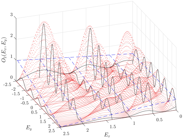
The oscillations of $T_{2}(E_{x},E_{y})$ continue out to large values of $\left|E_{y}-E_{x}\right|$ but are difficult to see in Fig. 3 because of the rapid decay of $T_{2}(E_{x},E_{y})$ with increasing $\left|E_{y}-E_{x}\right|$. To isolate the oscillatory behaviour, in Fig. 4 we plot the function

where

Here, $U_{2}(E_{x},E_{y})$ is essentially the denominator of $T_{L2}(E_{x},E_{y})$. Multiplying Eq. (20) by $U_{2}(E_{x},E_{y})$ we obtain

The solid black curves in Fig. 4 show numerical simulations of $O_{2}(E_{x},E_{y})$ for $N=5$ carried out using Eqs. (21), (22), (15) and (9) for the same values of $\Gamma$ and $k_{\mathrm{max}}$ as were used in Fig. 2 and 3. The numerical simulations and $O_{L2}(E_{x},E_{y})$ (dashed blue curves, see Eq. (23)) are shown along the lines $E_{x}=0$, $0.2a$, $0.4a$, $0.55a$, 0.8$a$ and 0.99$a$ and $E_{y}=-0.99a$ and $0.99a$. The red dots show $O_{H2}(E_{x},E_{y})=U_{2}(E_{x},E_{y})T_{H2}(E_{x},E_{y})$, the exact expression in terms of Hermite polynomials (see Eqs. (22) and (16)). The oscillations are visible for all values of $E_{x}$ and $E_{y}$ and the numerical simulations are seen to correctly reproduce the oscillations of the exact expression $O_{H2}(E_{x},E_{y})$. In can be seen that $O_{2}(0,E_{y})$ oscillates around an average value of $O_{L2}(0,E_{y})=\frac{1}{2}$ between $E_{y}=-a$ and $a$. However, since $O_{2}(E_{x},E_{y})$ oscillates in both the $E_{x}$ and $E_{y}$ directions there are valleys visible along which $O_{L2}(E_{x},E_{y})$ overestimates $O_{2}(E_{x},E_{y})$. In particular, $O_{L2}(E_{x},E_{y})$ overestimates $O_{2}(E_{x},E_{y})$ near the line $E_{x}=E_{y}$ and near the edges, where $T_{L2}(E_{x},E_{y})$ is singular. Previously, Kobayakawa et al. Kobayakawa1995 numerically investigated $-(E_{x}-E_{y})^{2}T_{2}(E_{x},E_{y})$ rather than $O_{2}(E_{x},E_{y})$ for generalisations of the GUE, GOE and GSE. In particular, these authors were interested in verifying numerically that the probability distribution of the matrix elements and corresponding level density only appear in the smoothed cluster function, Eq. (20), through the parameter $a$ which characterises the width of the spectrum.

Figs. 5 and 6 display semi-logarithmic plots of the two-point GUE cluster function $T_{2}(E_{x},E_{y})$ for $N=10$ along the lines $E_{x}=0$, $0.19a$, 0.44$a$, 0.736$a$ and 0.9999$a$ and $E_{y}=-0.9999a$ and $0.9999a$. The red solid curves show the exact result $T_{H2}(E_{x},E_{y})$ (Eq. (16)), the solid cyan curves show the approximation $T_{S2}(E_{x},E_{y})$ (Eq. (17)) and the dashed blue curves show the approximation $T_{L2}(E_{x},E_{y})$ (Eq. (20)). The solid black curves show the numerical simulations carried out using Eqs. (15) and (9) for ensemble size $k_{\mathrm{max}}=9\times 10^{7}$ with the delta function width $\Gamma=0.05$ in Fig. 5 and $\Gamma=0.4$ in Fig. 6. It is seen that when $\Gamma=0.05$ the numerical simulations follow the oscillations of the exact result $T_{H2}(E_{x},E_{y})$, but when the delta function width is increased to $\Gamma=0.4$ the numerical simulations follow the smooth behaviour of $T_{L2}(E_{x},E_{y})$ for large enough $\left|E_{y}-E_{x}\right|$. This transition corresponds to the transition which is observed in Fig. 1 for the average level density as $\Gamma$ is increased: the average level density changes from oscillating to smooth and lowers in the centre while rising at the edges. We mention two numerical artifacts which are visible in Figs. 5 and 6 which are related to the fact the density of levels is larger at the centre of the spectrum than the edges. First, in Fig. 5 the numerical simulations fail to correctly produce a smooth curve in the regions where $T_{2}(E_{x},E_{y})$ is smallest. This occurs because in these regions insufficient terms in the sums of delta functions in Eq. (15) make non-zero contributions; this could be fixed by using a larger ensemble. Second, in Fig. 6 the peaks in the numerical simulations at $E_{x}=E_{y}$ are artificially broad. This occurs be cause many more terms in the sums of delta functions in Eq. (15) make non-zero contributions in this region than at the edges resulting in the functional form used to represent the delta function (Eq. (9)) becoming visible more quickly at the centre than at the edges as the delta function width $\Gamma$ is increased. It may be possible fix this by using a smaller delta function width at the centre of the spectrum than at the edges but we do not explore this possibility here. We also note that the approximation $T_{S2}(E_{x},E_{y})$ is seen to correctly produce the oscillations of the exact result $T_{H2}(E_{x},E_{y})$ for small enough $\left|E_{y}-E_{x}\right|$ but to underestimate it near the edges.

Figs. 7 displays semi-logarithmic plots of the two-point GUE cluster function $T_{2}(E_{x},E_{y})$ for $N=100$ along the lines $E_{x}=0$, $0.2093a$, 0.452$a$, 0.7372$a$ and 0.9999$a$ and $E_{y}=-0.9999a$ and $0.9999a$. The numerical simulations were carried out for $k_{\mathrm{max}}=9\times 10^{6}$ and $\Gamma=1$. For this value of $\Gamma$ the numerical simulations follow the smooth behaviour of $T_{L2}(E_{x},E_{y})$ rather than the oscillatory behaviour of $T_{H2}(E_{x},E_{y})$. To correctly reproduce the oscillatory behaviour of $T_{H2}(E_{x},E_{y})$ with numerical simulations it is necessary to use a Gaussian broadened delta function width of no more than $\Gamma\sim 1/20$ while to obtain a smoothly varying cluster function for this order of $\Gamma$ it is necessary to use an ensemble of eigenvalues of size $k_{\mathrm{max}}\sim 10^{8}$. For $N=100$, an ensemble of eigenvalues of size $k_{\mathrm{max}}=10^{8}$ occupies 80 GB of computer memory and we were unable to perform the corresponding ensemble averages in a reasonable time with the computer which was available (9th generation Intel Core i9 with 64 GB of RAM). Again, the approximation $T_{S2}(E_{x},E_{y})$ is seen to correctly produce the oscillations of the exact result $T_{H2}(E_{x},E_{y})$ for small enough $\left|E_{y}-E_{x}\right|$ but to underestimate it near the edges.

Fig. 8 displays semi-logarithmic plots of the two-point GUE cluster function $T_{2}(E_{x},E_{y})$ for $N=1000$ for the same values of $E_{x}$ and $E_{y}$ as a fraction of $a$ as Fig. 7. The numerical simulations were carried out for $k_{\mathrm{max}}=9\times 10^{5}$ and $\Gamma=20$. For this value of $\Gamma$ the numerical simulations again follow the smooth behaviour of $T_{L2}(E_{x},E_{y})$ rather than the oscillatory behaviour of $T_{H2}(E_{x},E_{y})$. The exact expression for $T_{H2}(E_{x},E_{y})$ in terms of Hermite polynomials (Eq. (16)) does work numerically for $N=1000$ so no plot of $T_{H2}(E_{x},E_{y})$ is included in Fig. 8. The approximation $T_{S2}(E_{x},E_{y})$ is shown for comparison and can be seen to oscillate around $T_{L2}(E_{x},E_{y})$ except near the edges. In Figs. 5, 6, 7 and 8 it can seen that near the edges $T_{S2}(E_{x},E_{y})$ underestimates $T_{2}(E_{x},E_{y})$ while $T_{L2}(E_{x},E_{y})$ overestimates it. As explained in relation to Fig. 6, the artificially broad peaks which occur in the numerical simulations at $E_{x}=E_{y}$ are due to the large value of delta function width used ($\Gamma=20$). It was necessary to use such a large delta function width to compensate for the relatively small ensemble size used ($k_{\mathrm{max}}=9\times 10^{5}$). Artificially broad peaks at $E_{x}=E_{y}$ are also visible to a lesser extent in the numerical simulations of Fig. 7 for which $\Gamma=1$ and the ensemble size was $k_{\mathrm{max}}=9\times 10^{6}$.

Numerical simulations of the two-point eigenvalue correlation and cluster functions of the Gaussian unitary ensemble were carried out directly from their definitions by Eqs. (14) and (15) in terms of deltas functions. In Figs. 2 - 8, the numerical simulations are compared with analytical results which follow from three analytical formulas for the two-point GUE cluster function: (i) Eq. (16), (ii) Eq. (17) and (iii) Eq. (20). It is found that the oscillations present in formulas (i) and (ii) are reproduced by the numerical simulations if the the width of the function used to represent the delta function is small enough and that the non-oscillating behaviour of formula (iii) is approached as the width is increased.

It should be possible to use this method of numerically simulating two-point correlation and cluster functions to investigate for the range of validity of analytical results for other ensembles such as deformed ensembles Bertuola2005; Guhr1998 and to assist in the investigation of ensembles which are currently intractable analytically.

In this appendix we offer some considerations on the coding of the ensemble average in Eq. (14) for the two-point correlation function. Let us denote the $i$th eigenvalue of the $k$th realisation of the ensemble by $E_{ik}$ and define $N\times k_{\mathrm{max}}$ matrices $\verb!X!$ and $\verb!Y!$ whose elements are $\delta(E_{x}-E_{ik})$ and $\delta(E_{y}-E_{ik})$ respectively. Then the two-point correlation function $\verb!R!$ of energies $E_{x}$ and $E_{y}$ may be conveniently coded in Octave or Matlab by

where the $N\times N$ matrix $\verb!D!$ is the outer product of $\verb!X!$ and $\verb!Y'!$ (the transpose of $\verb!Y!$) and $\verb!sum(D(:))!$ is the grand sum of its elements.

References

- (1) J. Wishart, Biometrika 20A, 32 (1928)
- (2) E.P. Wigner, in Proceedings of the Fourth Canadian Mathematical Congress, Banff, 1957, ed. by M.S. Macphail (Univ. of Toronto Press, Toronto, 1959), pp. 174–184. Reprinted in Porter1965.
- (3) C.E. Porter, Statistical theories of spectra: fluctuations (Academic Press, N.Y., 1965)
- (4) T.A. Brody, J. Flores, J.B. French, P.A. Mello, A. Pandey, S.S.M. Wong, Rev. Mod. Phys. 53, 385 (1981)
- (5) G.E. Mitchell, A. Richter, H.A. Weidenmüller, Rev. Mod. Phys. 82, 2845 (2010)
- (6) H.A. Weidenmüller, G.E. Mitchell, Rev. Mod. Phys. 81, 539 (2009)
- (7) A.J. Sargeant, M.S. Hussein, A.N. Wilson, in Nuclei and Mesoscopic Physics: Workshop on Nuclei and Mesoscopic Physics; WNMP 2004, AIP Conf. Proc., vol. 777, ed. by V. Zelevinsky (2005), pp. 46–54
- (8) M.S. Hussein, B.V. Carlson, A.K. Kerman, Acta Phys. Pol. B 47, 391 (2016)
- (9) O. Bohigas, M.J. Giannoni, in Mathematical and computational methods in nuclear physics, Lecture Notes in Physics, vol. 209, ed. by J. Dehesa, J. Gomez, A. Polls (Springer, 1984), pp. 1–99
- (10) O. Bohigas, in Les Houches 1989 Session LII Chaos and quantum physics, ed. by M.J. Giannoni, A. Voros, J. Zinn-Justin (North Holland, Amsteram, 1991), pp. 87–199
- (11) M.A. Stephanov, J.J.M. Verbaarschot, T. Wettig, in Wiley Encyclopedia of Electrical and Electronics Engineering, ed. by J.G. Webster (Wiley, 1999)
- (12) C.W.J. Beenakker, Nucl. Phys. B 422, 515 (1994)
- (13) M.S. Hussein, J.G.G.S. Ramos, in Nuclei and Mesoscopic Physics 2017, AIP Conf. Proc., vol. 1912, ed. by P. Danielewicz, V. Zelevinsky (2017), p. 020007
- (14) J. Ambjørn, Y.M. Makeenko, Mod. Phys. Lett. A 5, 1753 (1990)
- (15) A. Edelman, B.D. Sutton, Y. Wang, in Modern Aspects of Random Matrix Theory, Proceedings of Symposia in Applied Mathematics, vol. 72, ed. by V.H. Vu (American Mathematical Society, 2014), pp. 53–82
- (16) B. Hayes, Am. Sci. 91, 296 (2003)
- (17) P.J. Forrester, A. Mays, Proc. R. Soc. Lond. A 471, 20150436 (2015)
- (18) M. Wolf, Rep. Prog. Phys. 83, 036001 (2020)
- (19) G. Ergün, in Encyclopedia of Complexity and Systems Science, ed. by R.A. Meyers (Springer, N.Y., 2009), pp. 7505–7520
- (20) F.J. Dyson, J. Math. Phys. 3, 166 (1962)
- (21) F.J. Dyson, M.L. Mehta, J. Math. Phys. 4, 701 (1963)
- (22) G. Livan, M. Novaes, P. Vivo, Introduction to random matrices: theory and practice (Springer, 2018)
- (23) E.P. Wigner, Distribution laws for the roots of a random Hermitean matrix (1962). Published in Porter1965.
- (24) M.L. Mehta, F.J. Dyson, J. Math. Phys. 4, 713 (1963)
- (25) B.V. Bronk, J. Math. Phys. 5, 215 (1964)
- (26) M. Mehta, Random matrices and the statistical theory of energy levels (Academic Press, N.Y., 1967)
- (27) J.M.G. Gómez, R.A. Molina, A. Relaño, J. Retamosa, Phys. Rev. E 66, 036209 (2002)
- (28) A.J. Sargeant, M.S. Hussein, M.P. Pato, M. Ueda, Phys. Rev. C 61, 011302 (2000)
- (29) H. Feshbach, Theoretical Nuclear Physics: Nuclear Reactions (Wiley, N.Y., 1992)
- (30) H. Pishro-Nik, Introduction to probability, statistics, and random processes (Kappa Research LLC, 2014). Available at https://www.probabilitycourse.com
- (31) Y.V. Fyodorov, in Recent Perspectives in Random Matrix Theory and Number Theory, ed. by F. Mezzadri, N.C. Snaith, London Mathematical Society Lecture Note Series (Cambridge University Press, 2005), pp. 31–78
- (32) E. Brézin, A. Zee, Nucl. Phys. B 402, 613 (1993)
- (33) E. Brézin, Physica A 221, 372 (1995)
- (34) J.B. French, P.A. Mello, A. Pandey, Ann. Phys. 113, 277 (1978)
- (35) A.M. Khorunzhy, B.A. Khoruzhenko, L.A. Pastur, J. Math. Phys. 37, 5033 (1996)
- (36) A. Pandey, Ann. Phys. 134, 110 (1981)
- (37) A.M.S. Macêdo, Phys. Rev. E 55, 1457 (1997)
- (38) Y. He, A. Knowles, Probab. Theory Relat. Fields 177, 147 (2020)
- (39) T.S. Kobayakawa, Y. Hatsugai, M. Kohmoto, A. Zee, Phys. Rev. E 51, 5365 (1995)
- (40) A.C. Bertuola, J.X. de Carvalho, M.S. Hussein, M.P. Pato, A.J. Sargeant, Phys. Rev. E 71, 036117 (2005)
- (41) T. Guhr, A. Müller-Groeling, H.A. Weidenmüller, Phys. Rep. 299, 189 (1998)