Stochastic Control and Pricing for Natural Gas Networks

A natural gas network is modeled as a directed graph comprising a set of nodes $\mathcal{N}=\{1,\dots,N\}$ and a set of edges $\mathcal{E}=\{1,\dots,E\}$. Nodes represent the points of gas injection, extraction or network junction, while edges represent pipelines. Each edge is assigned a direction from sending node $n$ to receiving node $n^{\prime}$, i.e., if $(n,n^{\prime})\in\mathcal{E}$, then $(n^{\prime},n)\notin\mathcal{E}$. The graph may contain cycles, while parallel edges and self-loops should not exist. The graph topology is described by a node-edge incidence matrix $A\in\mathbb{R}^{N\times E}$, such that

Let $\varphi\in\mathbb{R}^{E}$ be a vector of gas flow rates and let $\delta\in\mathbb{R}_{+}^{N}$ be a vector of gas extractions, which must be satisfied by the gas injections $\vartheta\in\mathbb{R}^{N}$ across the network given their injection limits $\underline{\vartheta},\overline{\vartheta}\in\mathbb{R}_{+}^{N}$. The gas conservation law is thus

The gas flow rates in network edges relate to the nodal pressures through non-linear, partial differential equations [16]. Under steady-state assumptions [13], however, the flows are related to pressures through the Weymouth equation:

where $\varrho\in\mathbb{R}^{N}$ is a vector of pressures contained within technical limits $\underline{\varrho},\overline{\varrho}\in\mathbb{R}_{+}^{N}$, and $w\in\mathbb{R}_{+}^{E}$ are constants that encode the friction coefficient and geometry of pipelines. To avoid non-linear pressure drops, let $\pi_{n}=\varrho_{n}^{2}$ be the squared pressure at node $n$ with limits $\underline{\pi}_{n}=\underline{\varrho}_{n}^{2}$ and $\overline{\pi}_{n}=\overline{\varrho}_{n}^{2}$.

To support the desired nodal pressures, the gas network operator regulates the pressure using active pipelines $\mathcal{E}_{a}\subset\mathcal{E}$, which host either compressors $\mathcal{E}_{c}\subset\mathcal{E}_{a}$ or valves $\mathcal{E}_{v}\subset\mathcal{E}_{a}$, assuming $\mathcal{E}_{c}\cap\mathcal{E}_{v}=\emptyset$. These network assets respectively increase and decrease the gas pressure along their corresponding edges. To rewrite the gas conservation law and Weymouth equation accounting for these components, let $\kappa\in\mathbb{R}^{E}$ be a vector of pressure regulation variables. Pressure regulation is non-negative $\kappa_{\ell}\geqslant 0$ for every compressor edge $\ell\in\mathcal{E}_{c}$ and it is non-positive $\kappa_{\ell}\leqslant 0$ for every valve edge $\ell\in\mathcal{E}_{v}$. This information is encoded in the pressure regulation limits $\underline{\kappa},\overline{\kappa}\in\mathbb{R}^{E}$. Pressure regulation involves an additional extraction of the gas mass to fuel active pipelines. Let matrix $B\in\mathbb{R}^{N\times E}$ relate the active pipelines to their sending nodes accounting for conversion factors, i.e.,

where $b_{\ell}$ is a conversion factor from the gas mass to the pressure regulation rate. The network equations become

Here, the gas extraction $B\kappa$ by compressor and valve edges in (1a) is always non-negative. Equation (1b) is the Weymouth equation in a vector form that accounts for both pressure loss and pressure regulation. The absolute value operator in (1b) is understood element-wise. Finally, equality (1c) enforces the unidirectional condition for the gas flow in active pipelines, because they permit the gas flow only in one direction.

The gas network optimization seeks the minimum of gas injection costs while satisfying gas flow equations and network limits. Let $c_{1}\in\mathbb{R}_{+}^{N}$ and $c_{2}\in\mathbb{R}_{+}^{N}$ be the coefficients of a quadratic gas injection cost function. With a perfect extraction forecast, the deterministic gas network optimization is

Despite the non-convexity of (2), it has been solved successfully using algorithmic solvers [17, 13] or general-purpose solvers [18] when all optimization parameters are known. These solvers no longer apply when the parameters are uncertain, because one needs to establish a convex dependency of optimization variables on uncertain parameters [19]. This convex dependency is established in this work by means of the linearization of the Weymouth equation (2c).

Let $\mathcal{W}(\varphi,\pi,\kappa)=\mathbb{0}$ denote the non-convex constraint (2c), and let $\mathcal{J}(x)\in\mathbb{R}^{E\times n}$ denote the Jacobian of (2c) w.r.t. an arbitrary vector $x\in\mathbb{R}^{n}$. The relation between the gas flow rates, nodal pressures, and pressure regulation rates can thus be approximated by the first-order Taylor series expansion:

where $(\mathring{\varphi},\mathring{\pi},\mathring{\kappa})$ is a stationary point retrieved by solving non-convex problem (2). As $\mathcal{W}(\mathring{\varphi},\mathring{\pi},\mathring{\kappa})=\mathbb{0}$ at a stationary point, equation (3) implies the affine relation:

where $\gamma_{1}\in\mathbb{R}^{E}$, $\gamma_{2}\in\mathbb{R}^{E\times N}$ and $\gamma_{3}\in\mathbb{R}^{E\times E}$ are coefficients encoding the sensitivity of gas flow rates to pressures and pressure regulation rates. These coefficients depend on the stationary point. For notational convenience, this dependency is dropped but always implied. In what follows, the Greek letter $\gamma$ denotes sensitivity coefficients and their transformations.

At the operational planning stage, well ahead of the real-time operations, the unknown gas extractions are modeled as

where $\delta\in\mathbb{R}^{N}$ is the mean value of the gas withdrawal rates and $\xi\in\mathbb{R}^{N}$ is a vector of zero-mean random forecast errors. Equation (5) suffices to model disturbances in gas extractions without an explicit modeling of gas consumption by gas-fired power plants in adjacent electrical power grids. We assume that the forecast error distribution $\mathbb{P}_{\xi}$ of $\xi$ and covariance $\Sigma=\mathbb{E}[\xi\xi^{\top}]$ can be estimated from the historical observations of electrical loads and renewable power generation, that are known to obey Normal, Log-Normal and Weibull distributions [20]. Though, more complex distributions may be envisaged for double-bounded stochastic processes of interest.

Regardless of the type and parameters of the uncertainty distribution, the chance-constrained counterpart of the deterministic gas network optimization in (2) writes as

which optimizes stochastic network variables $\tilde{\vartheta},\tilde{\kappa},\tilde{\varphi}$ and $\tilde{\pi}$ to minimize the expected value of the cost function (6a) subject to probabilistic constraints. The almost sure (a.s.) constraint (6b) requires the satisfaction of the gas conservation law and linearized Weymouth equation with probability 1, while the chance constraint (6c) ensures that the real-time pressures together with the injection, pressure regulation and flow rates remain within their technical limits. The prescribed violation probability $\varepsilon\in(0,1)$ reflects the risk tolerance of the gas network operator towards the violation of network limits.

The chance-constrained problem (6) is computationally intractable as it constitutes an infinite-dimensional optimization problem. To overcome its complexity, it has been proposed to approximate its solution by optimizing stochastic variables as affine, finite-dimensional functions of the random variable [4]. This functional dependency constitutes the model of the gas network response to uncertainty.

The explicit dependency on uncertainty is enforced on the controllable variables through the following affine policies

Equations (7) constitute the desired model of the network response to uncertainty. The model is said to be admissible if the stochastic gas conservation law and linearized Weymouth equation in (6b) hold with probability 1, i.e., for any realization of random variable $\xi$. This is achieved as follows.

The expected value of the gas network cost function in (6a) is computationally intractable as it involves an optimization of infinite-dimensional random variable $\tilde{\vartheta}(\xi)$. Under control policy (7a), however, we show that the computation of the expected cost reduces to solving an SOCP problem.

Due to definition of $\tilde{\vartheta}(\xi)$, function (6a) rewrites as

where the argument of the expectation operator is separable into nominal and random components. Due to the linearity of the expectation operator, it equivalently rewrites as

A zero-mean assumption made on distribution $\mathbb{P}_{\xi}$ factors out the first term under the expectation operator. The reformulation of the second term is made recalling that the expectation of the outer product of the zero-mean random variable yields its covariance, i.e., $\mathbb{E}[\xi\xi^{\top}]=\Sigma.$ Thus, the expected value of cost function (6a) reduces to a computation of

which is a convex quadratic function in variables $\vartheta$ and $\alpha$. To bring it to an SOCP form, let vectors $c^{\vartheta}\in\mathbb{R}^{N}$ and $c^{\alpha}\in\mathbb{R}^{N}$ substitute the quadratic terms of the gas injection and recourse costs. Moreover, let $F\in\mathbb{R}^{N\times N}$ be a factorization of covariance matrix $\Sigma$, such that $\Sigma=FF^{\top}$, and $\grave{c}_{2}\in\mathbb{R}^{N}$ be the factorization of vector $c_{2}$, such that $\text{diag}[c_{2}]=\grave{c}_{2}\grave{c}_{2}^{\top}$. Then, for any fixed values of nominal $\vartheta$ and recourse $\alpha$ decisions, the expected value of the cost is retrieved by solving the following SOCP problem

where (9b) and (9c) are rotated second-order cone constraints. Hence, the co-optimization of variables $\vartheta,\alpha,c^{\vartheta}$ and $c^{\alpha}$ results in the minimal expected cost. As problem (9) acts on a distribution-free response model (Remark 2), it does not require any assumption on the uncertainty distribution.

The optimization of response model (7) using the criterion of the minimum expected cost involves the risks of producing highly variable solutions for the state variables. See, for example, the evidences in the power system domain [21, 22]. However, since the state variables (7b) and (7c) are affine in control inputs, they can be optimized to provide the minimal-variance solution. To achieve the desired result, however, it is more suitable to optimize the standard deviations of the state variables as they admit conic formulations.

Let $s^{\pi}\in\mathbb{R}^{N}$ and $s^{\varphi}\in\mathbb{R}^{E}$ be the variables modeling the standard deviations of pressures and flow rates, respectively. For any fixed values of recourse decisions $\alpha$ and $\beta$, the standard deviations of pressures and flows rates are retrieved by solving the following SOCP problem

where (10b) and (10c) are second-order cone constraints, which are tight at optimality. Therefore, the co-optimization of variables $\alpha,\beta,s^{\pi}$ and $s^{\varphi}$ yields the optimized system response (7) that ensures the minimal-variance solution for the state variables. We finally note that this co-optimization is also distribution-free.

It remains to reformulate the joint chance constraint (6c) to attain a tractable reformulation. Given network response model (7), one way to satisfy (6c) is to enforce all its $N_{{\leqslant}}$ inequalities on a finite number of samples from $\mathbb{P}_{\xi}$ [23]. The sample-based reformulation, however, does not explicitly parameterize the problem by the risk tolerance $\varepsilon$ of the network operator. We thus proceed by enforcing individual chance constraints with the explicit analytic parameterization of the risk tolerance through individual violation probabilities $\hat{\varepsilon}\in\mathbb{R}_{+}^{N_{{\leqslant}}}$. This approach admits the Bonferroni approximation of the joint chance constraint in (6c) when $\mathbb{1}^{\top}\hat{\varepsilon}\leqslant\varepsilon$. The joint feasibility guarantee is provided even when the choice of the individual violation probabilities is sub-optimal [24], e.g. $\hat{\varepsilon}_{i}=\frac{\varepsilon}{N_{{\leqslant}}},\;\forall i=1,\dots,N_{{\leqslant}}$.

From [19] we know that a scalar chance constraint

where $z_{\hat{\varepsilon}}\geqslant 0$ is a safety parameter in the sense of [19], and the left-hand side of (11b) is the margin that ensures constraint feasibility given the parameters of the forecast errors distribution. Consequently, larger safety parameter $z_{\hat{\varepsilon}}$ improves system security. The choice of $z_{\hat{\varepsilon}}$ depends on the knowledge about distribution $\mathbb{P}_{\xi}$ [19], yet it always increases as the risk tolerance $\hat{\varepsilon}$ reduces.

Given the network response model (7) and the reformulations in (8)–(11), a computationally tractable version of stochastic problem (6) with the variance awareness formulates as the following SOCP problem:

in variables $\mathcal{P}=\{\vartheta,\kappa,\varphi,\pi,\alpha,\beta,c^{\vartheta},c^{\alpha},s^{\pi},s^{\varphi}\}$. Problem (12) optimizes the system response model (7) to meet a trade-off between the expected cost and the standard deviation of the state variables up to the given penalties $\psi^{\pi}\in\mathbb{R}_{+}^{N}$ and $\psi^{\varphi}\in\mathbb{R}_{+}^{E}$ for pressures and gas flow rates, respectively. Notice, that the constraints on the optimal recourse with respect to the reference node in (8d) are implicitly accounted for through the conic constraints on the gas injection and pressure regulation (12l)–(12o).

In formulation (12), the Greek letters $\lambda$ denote the dual variables of the coupling constraints. In the next Section IV, we invoke the SOCP duality theory to establish an efficient pricing scheme for gas networks under uncertainty.

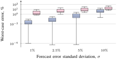
Lemma 1 hypothesizes the linear dependency of state variables on random forecast errors. Although the linear dependency enables a computationally tractable chance-constrained optimization in (12), it also leads to approximation errors due to non-convex relation between pressures, flows, and uncertain gas extraction rates. To ensure that the optimization of control policies in (7a) makes use of reliable state predictions, we develop a priori worst-case performance guarantees that the approximation errors do not exceed a certain threshold.

Since gas network congestions are mostly explained by pressure limits, we specifically focus on approximation errors associated with stochastic pressure variables. Let $\tilde{\pi}^{\star}(\xi)$ be the vector of the optimized stochastic pressures in (7b), i.e.,

which models the linear dependency on the optimal solution of problem (12), denoted by $\star$, and random forecast error $\xi$.

For some realization $\xi$, let $\pi^{\star}(\xi)$ be the actual pressure variables under control inputs from the optimized policies

where the optimal values are from the solution of problem (12). Pressure variables $\pi^{\star}(\xi)$ can be then retrieved by projecting the optimized control inputs from (14) to the non-convex feasible region specific to realization $\xi$, i.e, by solving

For any node $n\in\mathcal{N}$, the stochastic pressure approximation error can be then pre-computed as an Euclidean distance

between the approximation $\tilde{\pi}_{n}^{\star}(\xi)$ and the actual pressure variable $\pi_{n}^{\star}(\xi)$ for some forecast error realization $\xi$.

To provide the worst-case bound on the approximation error, we formulate the following optimization problem

in single variable $t$, which identifies that realization $\xi$ from $\mathbb{P}_{\xi}$, that results in the largest distance between the linear and non-convex stochastic pressure spaces. Observe, however, that constraint (17b) is infinite as it requires infinitely many samples from $\mathbb{P}_{\xi}$. Using a sample-based approach from [25], we provide the following finite counterpart of (17)

where $\widehat{\xi}_{s}$ is a discrete sample from $\mathbb{P}_{\xi}$, and constraint (18b) is enforced on a finite $S$ number samples (sample complexity), which is chosen to provide probabilistic performance guarantees with high confidence, as per the following Lemma.

We first study the optimized gas network response to uncertainty under deterministic and chance-constrained control policies (7a). The deterministic policies are optimized by setting the safety factor $z_{\hat{\varepsilon}}$ in problem (12) to zero. The policies are compared in terms of the expected cost (9a), the aggregated variance of gas pressures and flow rates $\sum_{n}\text{Var}[\tilde{\varrho}_{n}(\xi)]$ and $\sum_{\ell}\text{Var}[\tilde{\varphi}_{\ell}(\xi)]$ , respectively, and the total pressure regulation by compressors $\sum_{\ell\in\mathcal{E}_{c}}\sqrt{\kappa_{\ell}}$ and valves $\sum_{\ell\in\mathcal{E}_{v}}\sqrt{\kappa_{\ell}}$ . Note, we discuss the natural pressure quantities, not their squared counterparts used in optimization. The policies are also compared in terms of network constraints satisfaction. We first sample control inputs from (7) for $S=1,000$ realizations of forecast errors and count the violations of network limits (6c). Second, we assess the quality of the control inputs (7a) for the non-convex gas equations, by solving the projection problem (15) for all realizations $\xi_{s},\forall s=1,\dots,S$. A control input is considered feasible if (15a) is zero for a given realization. To characterize this infeasibility numerically, consider the average metrics $\mathcal{P}_{\text{inj}}=\sum_{s}\lVert\tilde{\vartheta}(\xi_{s})-\vartheta_{s}\rVert/S$ for gas injections and $\mathcal{P}_{\text{act}}=\sum_{s}\lVert\tilde{\kappa}(\xi_{s})-\kappa_{s}\rVert/S$ for active pipelines.

The results are reported in Table I. Disregarding uncertainty, the deterministic policies optimize the network operation for the nominal gas extraction rates and thus result in the minimum of cost at the operational planning stage. However, the produced control inputs are infeasible for most of the forecast error realizations. The projections $\mathcal{P}_{\text{inj}}$ and $\mathcal{P}_{\text{act}}$ of deterministic policies require the real-time correction of gas injections by $31.3$% and the real-time correction of pressure regulation by active pipelines by $12.7$% of the nominal rates on average. The chance-constrained policies, on the other hand, produce the control inputs that remain feasible with a probability at least $1-\varepsilon=99\%$ and require a minimal effort to restore the real-time gas flow feasibility. This real-time effort is non-zero due to approximation errors induced by linear pressure and flow equations of Lemma 1. Figure 2 illustrates the worst-case stochastic pressure approximation errors obtained according to the approach in Section III-F. The errors significantly depend on the amount of uncertainty: with probability $90\%$ and at high confidence, the errors approach 0% for a small uncertainty penetration level ($\sigma=1\%$), and they will not exceed 5.8% on average for the extremely large uncertainty penetration ($\sigma=10\%$). The errors under the deterministic solution, which ignores gas extraction uncertainty, are larger by at least an order of magnitude on average.

Table I further demonstrates that the variance-agnostic policy requires only a slight increase of the expected cost relative to the deterministic solution by $1.6$%, while the variance-aware policies allow to trade-off the expected operational cost for the smaller variations of pressures and flow rates. The variance of gas pressures and flow rates can be reduced by $63.8$% and $7.2$%, respectively, without any substantial impact on the expected cost. Observe that the subsequent variance reduction is achieved also due to the activation of valves in two active pipelines, that are not operating in the deterministic and variance-agnostic solutions.

With the density plots in Fig. 1, we demonstrate the uncertainty propagation through the network. The variance-agnostic solution results in the large pressure variance in the eastern part of the network with a large concentration of stochastic gas extractions. This solution further allows the probability of the gas flows reversal up to $11$% for certain pipelines, thus making the prediction of flow directions difficult. The variance-aware solution with the joint penalization of pressures and flows variance, in turn, drastically reduces the variation of the state variables and localizes the most of the variation only at nodes $34$ and $35$. Failure to minimize the pressure variance at these two nodes is due to relatively large approximation errors compared to the rest of the nodes (see the top quantiles of blue boxplots in Fig. 2). Although this variation remains large, the pressures at these nodes are highly correlated. Thus, by Weymouth equation (2c), the flow variance and the probability of flow reversal in edge $(34,35)$ remain small.

Next, we analyze the contribution of network assets to the variance control through the cost-variance trade-offs in Fig. 3. The figure illustrates these trade-offs when the control policies are assigned to gas injections only ($\alpha\in\text{free},\beta=\mathbb{0}$), to gas injections and compressors ($\alpha,\beta\in\text{free},[\beta]_{\ell}^{\top}=\mathbb{0},\forall\ell\in\mathcal{E}_{v}$), and to all network assets including valves ($\alpha,\beta\in\text{free}$). Observe that the variance reduction is achieved more rapidly and at lower costs as more active pipelines are involved into uncertainty and variance control. Hence, the stochastic control becomes more available as the network operator deploys more pressure regulation action by compressors and valves.

References

• [1] BP Energy Outlook, “2019 edition,” London, United Kingdom, 2019.
• [2] PJM Interconnection, “Analysis of operational events and market impacts during the January 2014 cold weather events,” 2014.
• [3] R. Bent et al., “Joint electricity and natural gas transmission planning with endogenous market feedbacks,” IEEE Trans. Power Syst., vol. 33, no. 6, pp. 6397–6409, 2018.
• [4] A. Ben-Tal, L. El Ghaoui, and A. Nemirovski, Robust optimization, vol. 28. Princeton University Press, 2009.
• [5] A. Shapiro, D. Dentcheva, and A. Ruszczyński, Lectures on stochastic programming: modeling and theory. SIAM, 2014.
• [6] L. A. Roald et al., “An uncertainty management framework for integrated gas-electric energy systems,” Proc. IEEE, 2020.
• [7] V. M. Zavala, “Stochastic optimal control model for natural gas networks,” Comput. Chem. Eng., vol. 64, pp. 103 – 113, 2014.
• [8] C. Ordoudis, “Market-based approaches for the coordinated operation of electricity and natural gas systems,” Ph.D. Thesis, 2018. Technical University of Denmark.
• [9] A. Ratha et al., “Affine policies for flexibility provision by natural gas networks to power systems,” Electr. Power Syst. Res., vol. 189, 2020. Article no. 106565.
• [10] C. Ordoudis et al., “Energy and reserve dispatch with distributionally robust joint chance constraints,” Technical Report, 2018. http://www.optimization-online.org/DB_FILE/2018/12/6962.pdf.
• [11] C. Wang et al., “Strategic offering and equilibrium in coupled gas and electricity markets,” IEEE Trans. Power Syst., vol. 33, no. 1, pp. 290–306, 2017.
• [12] C. Borraz-Sánchez et al., “Convex relaxations for gas expansion planning,” INFORMS J. Comput., vol. 28, no. 4, pp. 645–656, 2016.
• [13] M. K. Singh and V. Kekatos, “Natural gas flow solvers using convex relaxation,” IEEE Trans. Control. Netw. Syst., 2020. to be published.
• [14] A. Zlotnik et al., “Optimal control for scheduling and pricing intra-day natural gas transport on pipeline networks,” in 2019 IEEE CDC, pp. 4887–4884, 2019.
• [15] A. Zlotnik et al., “Pipeline transient optimization for a gas-electric coordination decision support system,” in PSIG Annual Meeting, Pipeline Simulation Interest Group, Jun 2019.
• [16] A. Thorley and C. Tiley, “Unsteady and transient flow of compressible fluids in pipelines—a review of theoretical and some experimental studies,” Int J Heat Fluid Flow, vol. 8, no. 1, pp. 3–15, 1987.
• [17] M. K. Singh and V. Kekatos, “Natural gas flow equations: Uniqueness and an MI-SOCP solver,” in 2019 IEEE ACC, pp. 2114–2120, 2019.
• [18] A. Wächter and L. T. Biegler, “On the implementation of an interior-point filter line-search algorithm for large-scale nonlinear programming,” Math. Program., vol. 106, no. 1, pp. 25–57, 2006.
• [19] A. Nemirovski and A. Shapiro, “Convex approximations of chance constrained programs,” SIAM J. Optim., vol. 17, no. 4, pp. 969–996, 2007.
• [20] K. N. Hasan, R. Preece, and J. V. Milanović, “Existing approaches and trends in uncertainty modelling and probabilistic stability analysis of power systems with renewable generation,” Renewable and Sustainable Energy Reviews, vol. 101, pp. 168–180, 2019.
• [21] D. Bienstock and A. Shukla, “Variance-aware optimal power flow: Addressing the tradeoff between cost, security, and variability,” IEEE Trans. Control. Netw. Syst., vol. 6, no. 3, pp. 1185–1196, 2019.
• [22] R. Mieth, J. Kim, and Y. Dvorkin, “Risk-and variance-aware electricity pricing,” Electr. Power Syst. Res., vol. 189, 2020. Article no. 106804.
• [23] M. C. Campi and S. Garatti, “The exact feasibility of randomized solutions of uncertain convex programs,” SIAM J. Optim., vol. 19, no. 3, pp. 1211–1230, 2008.
• [24] W. Xie, S. Ahmed, and R. Jiang, “Optimized bonferroni approximations of distributionally robust joint chance constraints,” Math. Program., pp. 1–34, 2019.
• [25] G. Calafiore and M. C. Campi, “Uncertain convex programs: randomized solutions and confidence levels,” Mathematical Programming, vol. 102, no. 1, pp. 25–46, 2005.
• [26] L. V. Kantorovich, “Mathematical methods of organizing and planning production,” Manage. Sci., vol. 6, no. 4, pp. 366–422, 1960.
• [27] P. A. Samuelson, “Spatial price equilibrium and linear programming,” The American Economic Review, vol. 42, no. 3, pp. 283–303, 1952.
• [28] S. Boyd, S. P. Boyd, and L. Vandenberghe, Convex optimization. Cambridge university press, 2004.
• [29] V. Dvorkin Jr, J. Kazempour, and P. Pinson, “Electricity market equilibrium under information asymmetry,” Oper. Res. Lett., vol. 47, no. 6, pp. 521–526, 2019.
• [30] S. Wu et al., “Model relaxations for the fuel cost minimization of steady-state gas pipeline networks,” Math. Comput. Modelling, vol. 31, no. 2, pp. 197 – 220, 2000.
• [31] Online repository: Stochastic Control and Pricing for Natural Gas Networks, 2020 (accessed October 5, 2020). https://github.com/anubhavratha/ng_stochastic_control_and_pricing.
• [32] I. Dunning, J. Huchette, and M. Lubin, “Jump: A modeling language for mathematical optimization,” SIAM Review, vol. 59, no. 2, pp. 295–320, 2017.
[Uncaptioned image] Vladimir Dvorkin (S’18, M’21) received a Ph.D. degree from the Technical University of Denmark, Lyngby, Denmark, in 2021. He is currently a postdoctoral associate with MIT Energy Initiative and Laboratory for Information and Decision Systems of Massachusetts Institute of Technology, Cambridge, MA, USA. His research interests include economics, game theory, optimization, and their applications to energy systems and markets.
[Uncaptioned image] Anubhav Ratha (S’18), received his M.Sc. degree in energy science and technology from ETH Zurich and is currently pursuing his PhD with the Department of Electrical Engineering, Technical University of Denmark. His research focus is on the design of market mechanisms and products for integrated energy systems of the future. Before his PhD studies, he co-founded a startup leveraging behavioral demand response to develop solutions for the green transition of electricity systems.
[Uncaptioned image] Pierre Pinson (SM’13, F’20) received his M.Sc. degree in applied mathematics from the National Institute for Applied Sciences, Toulouse, France, and the Ph.D. degree in energetics from Ecole des Mines de Paris, Paris, France. He is a Professor of Operations Research at the Department of Technology, Management and Economics of the Technical University of Denmark, Lyngby, Denmark. His research interests include forecasting, uncertainty estimation, optimization under uncertainty, decision sciences, and renewable energies. He is the Editor-in-Chief for the International Journal of Forecasting.
[Uncaptioned image] Jalal Kazempour (SM’18) received the Ph.D. degree in electrical engineering from the University of Castilla-La Mancha, Ciudad Real, Spain, in 2013. He is currently an Associate Professor with the Department of Electrical Engineering, Technical University of Denmark, Lyngby, Denmark. His focus area is the intersection of multiple fields, including power and energy systems, electricity markets, optimization, and game theory.