Fractonic superfluids (II): condensing subdimensional particles

In condensed matter systems, strong anisotropy can constrain particle’s propagation. For example, divergence of effective mass localizes particle spatially and a strong electric field allows charged particles to move exclusively along the direction of electric field. We have investigated one microscopic realization of fractons with fully restricted motion in Ref. Yuan et al. 2020. As a series of works, here we focus on $d$-component fields $\hat{\Phi}=(\hat{\Phi}_{1},\cdots,\hat{\Phi}_{d})$ in $d$ spatial dimensions in the Hamiltonian $H=\int\mathrm{d}^{d}\mathbf{x}\mathcal{H}$ where Hamiltonian density $\mathcal{H}$ reads

	$\displaystyle\mathcal{H}=$	$\displaystyle\sum_{a=1}^{d}\partial_{a}\hat{\Phi}_{a}^{{\dagger}}\partial_{a}\hat{\Phi}_{a}$
		$\displaystyle+\sum_{a\not=b}^{d}\frac{1}{2}K_{ab}(\hat{\Phi}_{a}^{{\dagger}}\partial_{a}\hat{\Phi}_{b}^{{\dagger}}+\hat{\Phi}_{b}^{{\dagger}}\partial_{b}\hat{\Phi}_{a}^{{\dagger}})\left(\hat{\Phi}_{a}\partial_{a}\hat{\Phi}_{b}+\hat{\Phi}_{b}\partial_{b}\hat{\Phi}_{a}\right)$
		$\displaystyle+V(\hat{\Phi}^{{\dagger}},\hat{\Phi})~.$		(1)

The complex fields $\hat{\Phi}_{a}^{{\dagger}}\left(\mathbf{x}\right)$ and $\hat{\Phi}_{b}\left(\mathbf{x}\right)$ create and annihilate an $a$th-component particle respectively and satisfy the bosonic communication relations

$$[\hat{\Phi}_{a}\left(\mathbf{x}\right),\hat{\Phi}_{b}^{{\dagger}}\left(\mathbf{y}\right)]=\delta_{ab}\delta^{d}\left(\mathbf{x-y}\right)\,,$$

(2)

where $\mathbf{x}=(x^{1},\cdots,x^{d})$ is the spatial coordinate. At the quadratic level, each component can only propagate in one certain spatial directions and we set the mass before the quadratic terms to be a unit. For convenience, one can set diagonal terms $K_{aa}=0$ for $a=1,\cdots,d$ since diagonal terms $K_{aa}$ is absent in Eq. (1). For simplicity, we can take the term $V(\hat{\Phi}^{\dagger},\hat{\Phi})$ to be the Mexican-hat potential with component-independent chemical potential $\mu$ and interaction coupling constant $g>0$ ,

$$V(\hat{\Phi}^{{\dagger}},\hat{\Phi})=\sum_{a=1}^{d}-\mu\hat{\Phi}_{a}^{{\dagger}}\hat{\Phi}_{a}+\frac{g}{2}\hat{\Phi}_{a}^{{\dagger}}\hat{\Phi}_{a}^{{\dagger}}\hat{\Phi}_{a}\hat{\Phi}_{a}$$

(3)

which describes a short-range repulsive interaction via the s-wave scattering. In the following, no Einstein summation rule is assumed. The Hamiltonian in Eq. (1) conserves both particle numbers of each components $Q_{a}\equiv\int\mathrm{d}^{d}x\hat{\rho}_{a}$ and angular charge moments $Q_{ab}=\int\mathrm{d}x^{d}(\hat{\rho}_{a}x^{b}-\hat{\rho}_{b}x^{a})$ with $\hat{\rho}_{a}=\hat{\Phi}_{a}^{\dagger}\hat{\Phi}_{a}$ being number operator of $a$th particles. Accordingly, the symmetry group is composed of transformations $\hat{\Phi}_{a}\rightarrow e^{i\lambda_{a}}\hat{\Phi}_{a}$ for each component and

$$(\hat{\Phi}_{a},\hat{\Phi}_{b})\rightarrow(\hat{\Phi}_{a}e^{i\lambda_{ab}x^{b}},\hat{\Phi}_{b}e^{-i\lambda_{ab}x^{a}})$$

(4)

for each pair of indices with $\lambda_{a},\lambda_{ab}\in\mathbb{R}$. The parameters $\lambda_{ab}$ are anti-symmetric $\lambda_{ab}=-\lambda_{ba}$, thus inducing $\frac{d(d-1)}{2}$ independent conserved angular charge moments $Q_{ab}$. The transformations in Eq. (4) involve local coordinates $\mathbf{x}=(x^{1},x^{2},\cdots,x^{d})$, and they do not form an internal symmetry. We denote the symmetry group as $\mathcal{G}$ which characterizes a higher-rank symmetry Seiberg 2020 . In a periodic boundary condition, the parameters $\lambda_{ab}$ have the dimension of $[x]^{-1}$ and quantization of the related charges is expected to coincide with a momentum. This symmetry intertwines global and internal symmetries such that strong constraints are imposed on particles’ propagations. In $2$D, conservation of $Q_{12}=\int\mathrm{d}^{2}x\left(\hat{\rho}_{1}x^{2}-\hat{\rho}_{2}x^{1}\right)$ requires the velocity shall be parallel to a vector $\left(\hat{\rho}_{1},\hat{\rho}_{2}\right)$ as a lineon. In three spatial dimensions, we have $3$ angular charge moments $Q_{12},Q_{23},Q_{13},$ such that a particle only propagates in the direction parallel to $\left(\hat{\rho}_{1},\hat{\rho}_{2},\hat{\rho}_{3}\right)$. Generally, fundamental particles in $d$D move with velocity parallel to $\left(\hat{\rho}_{1},\cdots,\hat{\rho}_{d}\right)$. Fig. 1 pictorially shows the interacting system when $d=2$.

It is well-known that a Bose-Einstein condensate consists of a two-component structure: the condensate and the normal components. The HFB mean-field theory allows factorization of fields $\hat{\Phi}_{a}$ in terms of an appropriate orthonormal single-particle basis,

$$\hat{\Phi}_{a}(\mathbf{x})=\phi_{a0}\left(\mathbf{x}\right)\hat{c}_{a0}+\sum_{i\not=0}\phi_{ai}\left(\mathbf{x}\right)\hat{c}_{ai}\equiv\phi_{a0}\left(\mathbf{x}\right)\hat{c}_{a0}+\hat{\psi}_{a}\left(\mathbf{x}\right)\,,$$

(5)

with $\hat{\psi}_{a}\left(\mathbf{x}\right)\equiv\sum_{i\not=0}\phi_{ai}\left(\mathbf{x}\right)\hat{c}_{ai}$ where the operator $\hat{c}_{ai}$ satisfies the bosonic commutation relations $[\hat{c}_{ai},\hat{c}_{bj}^{{\dagger}}]=\delta_{ab}\delta_{ij}$. The wavefunctions $\phi_{a0}\left(\mathbf{x}\right)$ signify the condensate component. The non-condensate fields $\hat{c}_{ai}\left(i\geq 1\right)$ constitute a branch of gapped quasiparticle excitations and are orthogonal with the condensate component $\phi_{a0}\left(\mathbf{x}\right),$

$$\int\mathrm{d}^{d}\mathbf{x}\phi_{a0}(\mathbf{x})\phi_{bi}^{\ast}(\mathbf{x})=0\text{ for }i\geq 1~.$$

(6)

Here the subscript index ‘$i$’ can be taken as a spectral index of the BdG Hamiltonian [see Eq. (16) ], and thus $\phi_{ai}$ can denote wave functions of low-energy excitations. We take the normal component as a perturbation to the condensate. Substituting Eq. (5) into Hamiltonian in Eq. (1) leads to a partition into terms with different numbers of field operators $\hat{\psi}_{a}(\mathbf{x})$. The zeroth-order term is given by

$$H_{0}=\sum_{a=1}^{d}h_{1,a}\hat{N}_{a0}+\sum_{a,b}h_{2,ab}(\hat{N}_{a0}\hat{N}_{b0}-\delta_{ab}\hat{N}_{a0})~,$$

(7)

where $\hat{N}_{a0}=\hat{c}_{a0}^{{\dagger}}\hat{c}_{a0}$ is the number operator for the condensate and $h_{1}\left(h_{2}\right)$ is the expectation value of the single-particle (two-particle) part of the Hamiltonian

	$\displaystyle h_{1,a}=$	$\displaystyle\int\mathrm{d}^{d}\mathbf{x}\left|\partial_{a}\phi_{a0}\right|^{2}-\mu\left|\phi_{a0}\right|^{2}~,$		(8)
	$\displaystyle h_{2,ab}=$	$\displaystyle\int\mathrm{d}^{d}\mathbf{x}\frac{1}{2}K_{ab}|\phi_{a0}\partial_{a}\phi_{b0}+\phi_{b0}\partial_{b}\phi_{a0}|^{2}$
		$\displaystyle+\frac{g\delta_{ab}}{2}\left|\phi_{a0}\phi_{b0}\right|^{2}.$		(9)

Under the particle-number representation $|\left\{N_{a0}\right\}\rangle$ with definite condensate particle number $\hat{N}_{b0}|\left\{N_{a0}\right\}\rangle=N_{b0}|\left\{N_{a0}\right\}\rangle$ for $b=1,\cdots,d$, the ground state energy $E_{0}\left(\left\{N_{a}\right\}\right)$ of $H_{0}$ in Eq. (7) only depends on the condensate,

	$\displaystyle E_{0}\left(\left\{N_{a}\right\}\right)$	$\displaystyle=\left\langle\left\{N_{a0}\right\}|H_{0}|\left\{N_{a0}\right\}\right\rangle$
		$\displaystyle=\sum_{a}h_{1,a}N_{a0}+\sum_{a,b}h_{2,ab}(N_{a0}N_{b0}-\delta_{ab}N_{a0})~.$		(10)

The next order $H_{1}$ has linear dependence on $\hat{\psi}_{a}\left(\mathbf{x}\right)$

$$H_{1}=\int\mathrm{d}^{d}\mathbf{x}\sum_{a=1}^{d}\hat{c}_{a0}^{{\dagger}}\phi_{a0}^{\ast}\mathcal{\hat{H}}_{a}^{{\dagger}}\hat{\psi}_{a}+\hat{\psi}_{a}^{{\dagger}}\mathcal{\hat{H}}_{a}\phi_{a0}\hat{c}_{a0}~,$$

(11)

where

$$\mathcal{\hat{H}}_{a}=-\partial_{a}^{2}-\mu+g\left|\phi_{a0}\right|^{2}\hat{N}_{a0}+\sum_{a,b}\frac{1}{2}K_{ab}\hat{N}_{b0}\mathcal{\hat{H}}_{ab}$$

(12)

with

	$\displaystyle\mathcal{\hat{H}}_{ab}=$	$\displaystyle(\partial_{a}\phi_{b0}^{\ast})(\partial_{a}\phi_{b0})+(\partial_{a}\phi_{b0}^{\ast})\phi_{b0}\partial_{b}-(\partial_{b}\phi_{b0}^{\ast})(\partial_{a}\phi_{b0})$
		$\displaystyle-\phi_{b0}^{\ast}(\partial_{a}\phi_{b0})\partial_{b}-\phi_{b0}^{\ast}(\partial_{a}\partial_{b}\phi_{b0})-(\partial_{b}\phi_{b0}^{\ast})\phi_{b0}\partial_{b}$
		$\displaystyle-\phi_{b0}^{\ast}(\partial_{b}\phi_{b0})\partial_{b}-\phi_{b0}^{\ast}\phi_{b0}\partial_{b}^{2}~.$

Under a basis $|\left\{N_{a0}\right\}\rangle$, taking the limit of $N_{a0}\gg 1$, one can recognize$\ \hat{N}_{a0}\hat{c}_{a0}|\left\{N_{a}\right\}\rangle=\hat{c}_{a0}\hat{N}_{a0}|\left\{N_{a}\right\}\rangle$. If $\phi_{a0}\left(\mathbf{x}\right)$ are chosen to be eigenstates of the operator $\mathcal{\hat{H}}_{a}$ in Eq. (12),

$$\mathcal{\hat{H}}_{a}\left(\mathbf{x}\right)\phi_{a0}\left(\mathbf{x}\right)=\epsilon_{a0}\left(\left\{N_{a0}\right\}\right)\phi_{a0}\left(\mathbf{x}\right)\,\,a=1,\cdots d~,$$

(13)

then $H_{1}$ vanishes identically due to orthogonality in Eq. (6) and $N_{a0}\gg 1$, where ground state energy $\epsilon_{a0}\left(\left\{N_{a0}\right\}\right)$ merely depends on the condensate component. This fact establishes the validity of the expansion in Eq. (5). The Eq. (13) marks a set of the GP equations describing the condensate components where $\mathcal{\hat{H}}_{a}$ in Eq. (12) behaves as a single-particle Hamiltonian. It simply directs us to approximate the original Hamiltonian in Eq. (1) by Eq. (7). With the translational symmetry, the GP equations have a set of very simple solutions. If the chemical potential $\mu$ is negative, the ground state energy $E_{0}$ reaches its minimum when the condensate has vanishing density, $N_{a0}=0$ for $a=1,\cdots d$. We obtain a normal state. If the chemical potential is switched to a positive value, the ground state energy $E_{0}$ reaches maximum with a finite number of the condensate component. In this case, the configurations of ground states can be parametrized by real parameters $\theta_{a}$ and $\beta_{ab}$ $(\beta_{ab}=-\beta_{ba},a,b=1,\cdots d)$,

$$\phi_{a0}\left(\mathbf{x}\right)=\frac{1}{\sqrt{V}}e^{i\left(\theta_{a}+\sum_{b=1}^{d}\beta_{ab}x^{b}\right)}~,$$

(14)

with $V$ as the spatial volume. Remarkably, Eq. (14) depends on the parameter $\beta_{ab}$ carrying the dimension of ‘momentum’. In other words, the condensate component can carry finite momentum. Of course, one can include the trap potential that can break a translational symmetry, under which the GP equations may be short of analytical solutions. Casting the solution in Eq. (14) back to $H_{0}$ in Eq. (7), we have the ground state energy $E_{0}\left(\left\{N_{a0}\right\}\right)$ ,

$$E_{0}\left(\left\{N_{a0}\right\}\right)=\sum_{a=1}^{d}-\mu\frac{N_{a0}}{V}+\frac{g}{2}\left(\frac{N_{a0}}{V}\right)^{2}~.$$

(15)

The minimal condition of $E_{0}\left(\left\{N_{a0}\right\}\right)$ with a positive chemical potential $\mu$ requires $\rho_{a0}\equiv\frac{N_{a0}}{V}=\frac{\mu}{g}$, which indicates the ground states for a fractonic superfluid has a macroscopically finite particle density. Hence, we obtain a superfluid phase by condensing lineons, which we dub $d\mathsf{SF}^{1}$. Therefore, select one ground state in Eq. (14) and we can fix the condensate particle number $N_{a0}$ by simply replacing both $\hat{c}_{a0}$ and $\hat{c}_{a0}^{{\dagger}}$ operators by c-number $\sqrt{N_{a0}}$, which indicates occurrence of ODLRO with the condensate density $\rho_{a0}$.

The next order $H_{2}$ goes beyond the GP equation to include the quadratic terms of $\psi_{a}$,

	$\displaystyle H_{2}$	$\displaystyle=\sum_{a=1}^{d}\int\mathrm{d}^{d}\mathbf{x}\hat{\psi}_{a}^{{\dagger}}(-\partial_{a}^{2}+g\rho_{a0})\hat{\psi}_{a}$
		$\displaystyle+\sum_{a,b}\frac{1}{2}K_{ab}\rho_{a0}\left(\partial_{a}\hat{\psi}_{b}^{{\dagger}}+\partial_{b}\hat{\psi}_{a}^{{\dagger}}\right)\left(\partial_{a}\hat{\psi}_{b}+\partial_{b}\hat{\psi}_{a}\right)$
		$\displaystyle+\sum_{a=1}^{d}\frac{g}{2}\rho_{a0}\left(\hat{\psi}_{a}^{{\dagger}}\hat{\psi}_{a}^{{\dagger}}+\hat{\psi}_{a}\hat{\psi}_{a}\right)\,,$		(16)

where we have replaced $\hat{c}_{a0}$ and $\hat{c}_{a0}^{{\dagger}}$ with $\sqrt{N_{a0}}$. New quadratic terms emerge from $K_{ab}$-term which relaxes the restrictions on dynamics. It means that the quasiparticle modes $\hat{\psi}_{a}$ can propagate along all spatial directions. The mass term $g\rho_{a0}\hat{\psi}_{a}^{{\dagger}}\hat{\psi}_{a}$ originates from the condensate component. $H_{2}$ in Eq. (16) is designated as a BdG Hamiltonian to characterize the non-condensate quasiparticle modes. One can diagonalize $H_{2}$ to obtain the canonical quaisparticle modes. For example, in $2$D, the spectrum has two branches,

$$\epsilon_{\pm}=\sqrt{\left[\frac{(1+K\rho_{0})|\mathbf{k}|^{2}}{2}\pm\frac{\Delta(\mathbf{k})}{2}+g\rho_{0}\right]^{2}-(g\rho_{0})^{2}}~.$$

(17)

For small momentum, up to the first order, we have linear gapless dispersion relations,

$$\epsilon_{\pm}(\mathbf{k})=\sqrt{g\rho_{0}}\sqrt{(1+K\rho_{0})\mathbf{k}^{2}\pm\Delta(\mathbf{k})}\quad\mathrm{small}~\mathbf{k}~,$$

(18)

and they describe two gapless phonon excitations, while at the large momentum, spectrum dispersions depend on momentum quadratically,

$\displaystyle\epsilon_{\pm}=\frac{(1+K\rho_{0})|\mathbf{k}|^{2}}{2}\pm\frac{\Delta(\mathbf{k})}{2}\quad\mathrm{large}~\mathbf{k}~,$

(19)

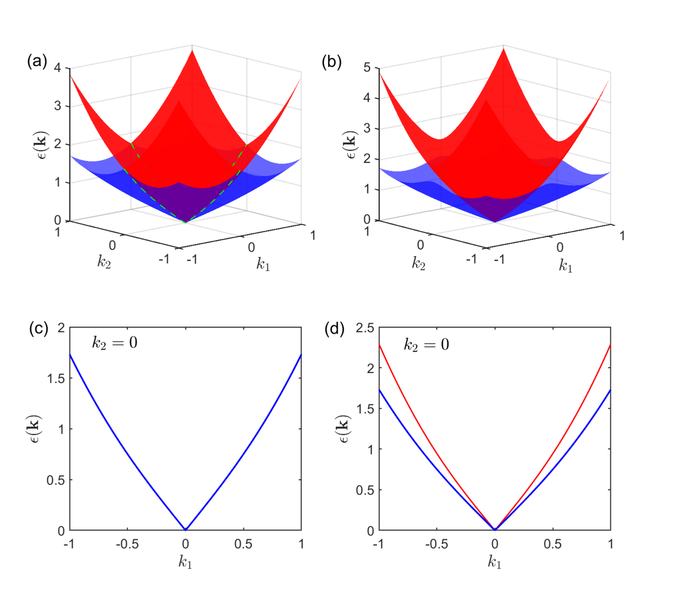
and instead they correspond to gapped roton modes. Here $\Delta(\mathbf{k})\equiv\sqrt{\left(k_{1}^{2}-k_{2}^{2}\right)^{2}\left(K\rho_{0}-1\right)^{2}+4K^{2}\rho_{0}^{2}k_{1}^{2}k_{2}^{2}}$, $\rho_{0}=\frac{\mu}{g}$ and $K\equiv K_{12}$. The smooth change from linear to quartic dispersion is the key feature of the HFB approximation. Although two modes, phonons and rotons, are emphasized, indeed they represent different behavors at small and high momentum respectively. The splitting between the two dispersion relations in Eqs. (18) and (19) is controlled by $\Delta(\mathbf{k})$. If $K\rho_{0}=1$ such that $\Delta(\mathbf{k})=0$, the two bands are degenerate at two lines $k_{1}=0$ or $k_{2}=0$ and along the two lines, the bands have ill-defined curvatures, which is expected to be detected by thermal Hall effect. Figure 2 depicts the two dispersion relations in Eq. (17) in which the two cases of $K\rho_{0}=1$ or not.

Higher-order terms couple the normal with the condensate part and describe the interaction between phonon modes, which is beyond the scope of this work and we leave it to future work.

For the coherence and completeness of the present section, we re-derive some quantities from the field-theoretical perspective.

We perform a coherent-state path integral quantization Altland and Simons 2010 to get the Lagrangian density $\mathcal{L}$,

$$\mathcal{L}=\sum_{a=1}^{d}i\phi_{a}^{\ast}\partial_{t}\phi_{a}-\mathcal{H}\left(\phi\right)~,$$

(20)

where $\phi_{a}(\mathbf{x},t)$ is an eigenvalue of $\hat{\Phi}_{a}(\mathbf{x})$ on a coherent state $\hat{\Phi}_{a}(\mathbf{x})|\phi_{a}(\mathbf{x},t)\rangle=\phi_{a}(\mathbf{x},t)|\phi_{a}(\mathbf{x},t)\rangle$. The first order derivative in Eq. (20) in nature is determined by the commutation relation in Eq. (2) which can be confirmed through the canonical quantization. For convenience, we apply the Wick’s rotation to an imaginary time at zero temperature $T=0$.

Next, we can derive the Euler-Lagrange equations as well as the Noether currents associated with two types of conserved quantities. The Euler-Lagrange equations can be derived from the formula $\frac{\delta\mathcal{L}}{\delta\phi_{a}^{\ast}}=0$, explicitly, $i\partial_{t}\phi_{a}=\hat{H}_{a}\phi_{a}~(a=1,\cdots,d)$, where $\hat{H}_{a}$ has the same form as $\mathcal{H}_{a}$ in Eq. (12),

$$\hat{H}_{a}=-\partial_{a}^{2}-\mu+g\left|\phi_{a}\right|^{2}+\frac{1}{2}\sum_{b}\mathcal{H}_{ab}~.$$

(21)

Here $\mathcal{H}_{ab}$ comes from the $K_{ab}$-term,

	$\displaystyle\mathcal{H}_{ab}=$	$\displaystyle K_{ab}\partial_{a}\phi_{b}^{\ast}\partial_{a}\phi_{b}+K_{ab}\partial_{a}\phi_{b}^{\ast}\phi_{b}\partial_{b}-K_{ab}\partial_{b}\phi_{b}^{\ast}\partial_{a}\phi_{b}$
		$\displaystyle-K_{ab}\phi_{b}^{\ast}\partial_{a}\phi_{b}\partial_{b}-K_{ab}\phi_{b}^{\ast}\partial_{a}\partial_{b}\phi_{b}-K_{ab}\partial_{b}\phi_{b}^{\ast}\phi_{b}\partial_{b}$
		$\displaystyle-K_{ab}\phi_{b}^{\ast}\partial_{b}\phi_{b}\partial_{b}-K_{ab}\phi_{b}^{\ast}\phi_{b}\partial_{b}^{2}\,.$		(22)

The Euler-Lagrange equations just recover the GP equations. Here $\phi_{a}$ plays the same role of representing the condensate component as $\phi_{a0}$ in Eq. (13).

The Hamiltonian in Eq. (1) stays invariant under transformation in Eq. (4) as well as the particle number conservation symmetry. For the infinitesimal change $\delta\phi_{a}=i\alpha_{a}\phi_{a}$, we have the related Noether charge $Q_{a}$ with charge density $\rho_{a}$ and currents $J_{i}^{a}$ that read,

	$\displaystyle Q^{a}=$	$\displaystyle\int\mathrm{d}^{d}\mathbf{x}\phi_{a}^{\ast}\phi_{a}\equiv\int\mathrm{d}^{d}\mathbf{x}\rho_{a}$		(23)
	$\displaystyle J_{i}^{a}=$	$\displaystyle iK_{ai}\rho_{a}\left(\phi_{i}\partial_{a}\phi_{i}^{\ast}-\phi_{i}^{\ast}\partial_{a}\phi_{i}\right)$
		$\displaystyle+iK_{ai}\rho_{i}\left(\phi_{a}\partial_{i}\phi_{a}^{\ast}-\phi_{a}^{\ast}\partial_{i}\phi_{a}\right)$
		$\displaystyle+i\left(\phi_{i}\partial_{i}\phi_{i}^{\ast}-\phi_{i}^{\ast}\partial_{i}\phi_{i}\right)\delta_{ai}$		(24)

which satisfies the continuity equations $\partial_{t}\rho^{a}+\sum_{i}\partial_{i}J_{i}^{a}=0$. Here in Eq. (23), coincidence between $\phi_{a}^{*}\phi_{a}$ and particle density $\rho_{a}$ arises from the first-order time derivative in Hamiltonian in Eq. (1). For the transformation $\delta\phi_{a}=ix_{b}\phi_{a}$ and $\delta\phi_{b}=-ix_{a}\phi_{b}$ corresponding to Eq. (4), we have conserved angular moments $Q_{ab}$ (with density $\rho_{ab}$) and currents $D_{i}^{ab}$,

	$\displaystyle Q_{ab}$	$\displaystyle=\int\mathrm{d}^{d}x\left(\rho_{a}x^{b}-\rho_{b}x^{a}\right)\equiv\int\mathrm{d}^{d}x\rho_{ab}$		(25)
	$\displaystyle D_{i}^{ab}$	$\displaystyle=x^{b}J_{i}^{a}-x^{a}J_{i}^{b}$		(26)

with $\rho_{a}$ and $J_{i}^{a}$ as $U(1)$ charge and current in Eqs. (23) and (24). The continuity equation $\partial_{t}\rho^{ab}+\sum_{i=1}^{d}\partial_{i}D_{i}^{ab}=0$ is automatically satisfied as long as the currents $J_{b}^{a}$ obey the relations $J_{b}^{a}=J_{a}^{b}$.

The HFB mean-field theory in Sec. II.2 starts with one of the classical field configurations $\phi_{a}^{\textrm{cl}}=\sqrt{\rho_{0}}e^{(i\theta_{a}+i\sum_{b=1}^{d}\beta_{ab}x^{b})}$ which can be formulated in the second quantization language as

$\displaystyle\!\!\!\!|\text{GS}\rangle_{\theta_{a}}^{\beta_{ab}}=\prod\limits_{a=1}^{d}\exp[\sqrt{\rho_{0}}e^{i\left(\theta_{a}+\sum_{b=1}^{d}\beta_{ab}x^{b}\right)}\hat{\Phi}_{a}^{{\dagger}}\left(\mathbf{x}\right)]|0\rangle~,$

(27)

where $\hat{\Phi}_{a}^{{\dagger}}(\mathbf{x})$ $\left(a=1,\cdots,d\right)$ creates an $a$th-component lineon with restricted motion. The salience of Eq. (27) features a finite expectation value of operator $\hat{\Phi}_{a}(\mathbf{x})$

$$\langle\mathrm{GS}|\hat{\Phi}_{a}(\mathbf{x})|\mathrm{GS}\rangle_{\theta_{a}}^{\beta_{ab}}=\sqrt{\rho_{0}}\exp(i\theta_{a}+i\sum_{b}\beta_{ab}x^{b})~,$$

(28)

thus marking an ODLRO and we obtain a fractonic superfluid phase $d\mathsf{SF}^{1}$. The expectation value oscillates as a plane-wave with fixed momentum $\mathbf{k}_{a}=\left(\beta_{a1},\beta_{a2},\cdots,\beta_{ad}\right)$ for the $a$-component particle. In this sense, we can rewrite $|\mathrm{GS}\rangle_{\theta_{a}}^{\beta_{ab}}=\prod\limits_{a=1}^{d}\exp\left[\sqrt{\rho_{0}}e^{i\theta_{a}}\hat{\Phi}_{a}^{{\dagger}}(\mathbf{k}_{a})\right]|0\rangle$ with $\hat{\Phi}_{a}^{{\dagger}}\left(\mathbf{k}_{a}\right)$ being the Fourier transformation of $\hat{\Phi}_{a}^{{\dagger}}(\mathbf{x})$. These features arise from restricted mobility of condensed particles. As a side note, the ground state in Eq. (27), which carries finite momentum, looks like a Fulde–Ferrell–Larkin–Ovchinnikov (FFLO) state Fulde and Ferrell 1964; Larkin and Ovchinnikov 1964. However, the general FFLO states are formed by Cooper pairs of fermions condensing at finite momentum. In contrast, the superfluid phase in Eq. (27) are directly formed by condensation of multi-component bosonic lineons. The degenerate ground state subspace is generated by group elements of higher-rank symmetry group $\mathcal{G}$ (see Sec. II.1).

After condensation, the Noether currents in Eqs. (24) and (26) reduce to simpler forms by expanding the field $\phi_{a}=\phi_{a}^{\text{cl}}e^{i\theta_{a}}$ where $\phi_{a}^{\text{cl}}$ denotes classical configurations and $\theta_{a}$ are the quantum phase fluctuations,

$\displaystyle\rho_{a}=\rho_{0}\,,J_{i}^{a}=2K\rho_{0}^{2}\left(\partial_{i}\theta_{a}+\partial_{a}\theta_{i}\right)+2\rho_{0}\partial_{i}\theta_{a}\delta_{ai}\text{ }$

(29)

and

$\displaystyle\rho_{ab}=\rho_{0}\left(x^{b}-x^{a}\right)\,,D_{i}^{ab}=x^{b}J_{i}^{a}-x^{a}J_{i}^{b}\,.$

(30)

To derive the effective theory for quantum fluctuations or the gapless Goldstone modes, we expand the fields around a selected classical configuration $\phi_{a}\left(\mathbf{x},t\right)=\sqrt{\rho_{0}+\rho_{a}\left(\mathbf{x},t\right)}e^{i\theta_{a}\left(\mathbf{x},t\right)}$ where $\rho_{a}$ and $\theta_{a}$ denote density and phase fluctuations respectively. Up to the second order, we have

	$\displaystyle\mathcal{L}$	$\displaystyle=\sum_{a=1}^{d}-\rho_{a}\partial_{t}\theta_{a}-\rho_{0}\left(\partial_{a}\theta_{a}\right)^{2}-\frac{1}{4\rho_{0}}\left(\partial_{a}\rho_{a}\right)^{2}-\frac{g}{2}\rho_{a}^{2}$
		$\displaystyle-\sum_{a,b}\frac{1}{2}K_{ab}\rho_{0}^{2}\left(\partial_{a}\theta_{b}+\partial_{b}\theta_{a}\right)^{2}$
		$\displaystyle-\frac{1}{8}\sum_{a,b}K_{ab}\left(\partial_{a}\rho_{b}+\partial_{b}\rho_{a}\right)^{2}\,.$		(31)

The density fluctuation fields $\rho_{a}$ $(a=1,\cdots,d)$ work as auxiliary fields that are subject to the constraint equations

	$\displaystyle\partial_{t}\theta_{a}=$	$\displaystyle-g\rho_{a}-\left(\frac{1}{2\rho_{0}}\partial_{a}^{2}+\frac{1}{2}\sum_{b}K_{ab}\partial_{b}^{2}\right)\rho_{a}$
		$\displaystyle-\frac{1}{2}\sum_{b}K_{ab}\partial_{a}\partial_{b}\rho_{b}~.$		(32)

Since we are only interested in the low-energy physics, the momentum $\mathbf{k}$ has an upper bound $\left|\mathbf{k}\right|\leq 2\pi\xi_{c}^{-1}$ where the coherent length $\xi_{c}$ can be estimated as

$$g=4\pi^{2}\xi_{c}^{-2}\left(\frac{1}{2\rho_{0}}+\sum_{b}K_{ab}\right)$$

(33)

as such the last two terms in Eq. (32) can be neglected. In the low-energy limit, we obtain the solutions $\rho_{a}=-\frac{1}{g}\partial_{t}\theta_{a}$. Cast it back to Eq. (31) and we arrive at an effective theory of quantum fluctuations by excluding the higher derivative terms of $\theta_{a}$,

	$\displaystyle\mathcal{L}=$	$\displaystyle\sum_{a}\frac{1}{2g}\left(\partial_{t}\theta_{a}\right)^{2}-\rho_{0}\left(\partial_{a}\theta_{a}\right)^{2}$
		$\displaystyle-\sum_{a,b}\frac{1}{2}K_{ab}\rho_{0}^{2}\left(\partial_{a}\theta_{b}+\partial_{b}\theta_{a}\right)^{2}~.$		(34)

The effective theory in Eq. (34) stays invariant under the transformation $\theta_{a}\rightarrow\theta_{a}+\lambda_{a}+\sum_{b}\lambda_{ab}x^{b}$ with $\lambda_{ab}=-\lambda_{ba}$. It describes $d$ gapless Goldstone modes $\theta_{a}\left(a=1,\cdots,d\right)$ Watanabe 2020 that have entangled motions arising from $K_{ab}$ term.

To get a deeper insight, we concentrate ourselves on the $2$D case. Introduce the canonical modes $\Theta_{+}\left(\mathbf{k}\right)$ and $\Theta_{-}\left(\mathbf{k}\right)$

	$\displaystyle\Theta_{+}\left(\mathbf{k}\right)$	$\displaystyle=\cos\frac{\varphi_{\mathbf{k}}}{2}\theta_{1}\left(\mathbf{k}\right)+\sin\frac{\varphi_{\mathbf{k}}}{2}\theta_{2}\left(\mathbf{k}\right)\,,$		(35)
	$\displaystyle\Theta_{-}\left(\mathbf{k}\right)$	$\displaystyle=-\sin\frac{\varphi_{\mathbf{k}}}{2}\theta_{1}\left(\mathbf{k}\right)+\cos\frac{\varphi_{\mathbf{k}}}{2}\theta_{2}\left(\mathbf{k}\right)\,,$		(36)

where $\tan\frac{\varphi_{\mathbf{k}}}{2}=\frac{2K\rho_{0}k_{1}k_{2}}{\Delta\left(\mathbf{k}\right)^{2}}$ with denoting $K_{12}=K$ and their dispersion relations take the form as $\epsilon_{\pm}\left(\mathbf{k}\right)=\sqrt{g\rho_{0}\left[\left(1+K\rho_{0}\right)\mathbf{k}^{2}\pm\Delta\left(\mathbf{k}\right)\right]}$, which is identical to Eq. (18).

Stability of a superfluid phase is determined by the long-distance behavor of the correlator of the order parameter under the influence of by quantum fluctuations,

		$\displaystyle\langle\text{GS}|\Phi_{a}^{{\dagger}}\left(\mathbf{x}\right)\Phi_{b}\left(\mathbf{0}\right)|\text{GS}\rangle_{\theta_{a}}^{\beta_{ab}}$
	$\displaystyle=$	$\displaystyle\rho_{0}\exp[i\sum_{c}(\beta_{bc}-\beta_{ac})x^{c}]\left\langle e^{-i\Theta_{a}(\mathbf{x})}e^{i\Theta_{b}(\mathbf{0})}\right\rangle~.$		(37)

We need to calculate equal-time correlators of the canonical modes $\left\langle e^{-i\Theta_{\pm}\left(\mathbf{x}\right)}e^{i\Theta_{\pm}\left(\mathbf{0}\right)}\right\rangle=e^{-\frac{1}{2}\langle[\Theta_{\pm}(\mathbf{x})-\Theta_{\pm}(\mathbf{0})]^{2}\rangle}$. Explicitly, in two spatial dimensions, we have

		$\displaystyle\left\langle\Theta_{\pm}\left(\mathbf{x}\right)\Theta_{\pm}(\mathbf{0})\right\rangle$
	$\displaystyle=$	$\displaystyle\int\frac{\mathrm{d}\omega\mathrm{d}^{2}k}{\left(2\pi\right)^{3}}\frac{e^{i\mathbf{k\cdot x}}}{\omega^{2}-\omega_{\pm}\left(\mathbf{k}\right)}$
	$\displaystyle=$	$\displaystyle\int\frac{\mathrm{d}k\mathrm{d}\theta}{(2\pi)^{2}}\frac{e^{ik|\mathbf{x}|\cos\theta}}{\sqrt{g\rho_{0}\left[\left(1+K\rho_{0}\right)\pm\bar{\Delta}\left(\theta\right)\right]}}$
	$\displaystyle<$	$\displaystyle\int\frac{\mathrm{d}k\mathrm{d}\theta}{(2\pi)^{2}}\frac{e^{ik|\mathbf{x}|\cos\theta}}{\sqrt{g\rho_{0}c_{\pm}}}=\frac{1}{2\pi|\mathbf{x}|}\frac{1}{\sqrt{g\rho_{0}c_{\pm}}}\,,$		(38)

where $\bar{\Delta}(\theta)=\sqrt{(1-2K\rho_{0})\cos^{2}2\theta+K^{2}\rho_{0}^{2}}$ and $c_{\pm}$ denotes the minimum value of $(1+K\rho_{0})\pm\bar{\Delta}(\theta)$. At the long distance $|\mathbf{x}|\rightarrow\infty$, the correlator $\left\langle\Theta_{\pm}\left(\mathbf{x}\right)\Theta_{\pm}(\mathbf{0})\right\rangle$ vanishes. Thus, $\left\langle\Phi_{a}^{{\dagger}}\left(\mathbf{x}\right)\Phi_{b}\left(\mathbf{0}\right)\right\rangle=\rho_{0}\exp[i\sum_{c}(\beta_{bc}-\beta_{ac})x^{c}]$ has a finite value modulated by a plane wave. It confirms a true long-range order that survives against quantum fluctuations when both the two lineons condensate simultaneously in zero temperature. Since quantum fluctuations are weaker in higher dimensions, a fractonic superfluid phase $d\mathsf{SF}^{1}$ stays stable in two spatial dimensions $d=2$ and higher $d>2$. In Appendix A, the component-dependent Mexican-hat potential in $2$D is considered, which leads to condensation of only one component of lineons. The uncondensed component gets released from mobility restriction and the Goldstone mode behaves still as a subdimensional particle. Thus, the superfluid there obeys an algebraic order.

References

- Chamon (2005) Claudio Chamon, “Quantum glassiness in strongly correlated clean systems: An example of topological overprotection,” Phys. Rev. Lett. 94, 040402 (2005).
- Haah (2011) Jeongwan Haah, “Local stabilizer codes in three dimensions without string logical operators,” Phys. Rev. A 83, 042330 (2011).
- Vijay et al. (2015) Sagar Vijay, Jeongwan Haah, and Liang Fu, “A new kind of topological quantum order: A dimensional hierarchy of quasiparticles built from stationary excitations,” Phys. Rev. B 92, 235136 (2015).
- Vijay et al. (2016) Sagar Vijay, Jeongwan Haah, and Liang Fu, “Fracton topological order, generalized lattice gauge theory, and duality,” Phys. Rev. B 94, 235157 (2016).
- Prem et al. (2017) Abhinav Prem, Jeongwan Haah, and Rahul Nandkishore, “Glassy quantum dynamics in translation invariant fracton models,” Phys. Rev. B 95, 155133 (2017).
- Shirley et al. (2019) Wilbur Shirley, Kevin Slagle, and Xie Chen, “Foliated fracton order from gauging subsystem symmetries,” SciPost Phys. 6, 41 (2019).
- Ma et al. (2017) Han Ma, Ethan Lake, Xie Chen, and Michael Hermele, “Fracton topological order via coupled layers,” Phys. Rev. B 95, 245126 (2017).
- Bulmash and Barkeshli (2019) Daniel Bulmash and Maissam Barkeshli, “Gauging fractons: Immobile non-Abelian quasiparticles, fractals, and position-dependent degeneracies,” Phys. Rev. B 100, 155146 (2019), arXiv:1905.05771 [cond-mat.str-el] .
- Prem and Williamson (2019) Abhinav Prem and Dominic Williamson, “Gauging permutation symmetries as a route to non-Abelian fractons,” SciPost Physics 7, 068 (2019), arXiv:1905.06309 [cond-mat.str-el] .
- Bulmash and Barkeshli (2018) D. Bulmash and M. Barkeshli, “Generalized Gauge Field Theories and Fractal Dynamics,” arXiv e-prints (2018), arXiv:1806.01855 [cond-mat.str-el] .
- Tian et al. (2020) Kevin T. Tian, Eric Samperton, and Zhenghan Wang, “Haah codes on general three-manifolds,” Annals of Physics 412, 168014 (2020), arXiv:1812.02101 [quant-ph] .
- You et al. (2019) Yizhi You, Daniel Litinski, and Felix von Oppen, “Higher-order topological superconductors as generators of quantum codes,” Phys. Rev. B 100, 054513 (2019), arXiv:1810.10556 [cond-mat.str-el] .
- Ma et al. (2018) Han Ma, Michael Hermele, and Xie Chen, “Fracton topological order from the higgs and partial-confinement mechanisms of rank-two gauge theory,” Phys. Rev. B 98, 035111 (2018).
- Slagle and Kim (2017) Kevin Slagle and Yong Baek Kim, “Fracton topological order from nearest-neighbor two-spin interactions and dualities,” Phys. Rev. B 96, 165106 (2017).
- Halász et al. (2017) Gábor B. Halász, Timothy H. Hsieh, and Leon Balents, “Fracton topological phases from strongly coupled spin chains,” Phys. Rev. Lett. 119, 257202 (2017).
- Tian and Wang (2019) Kevin T. Tian and Zhenghan Wang, “Generalized Haah Codes and Fracton Models,” arXiv e-prints , arXiv:1902.04543 (2019), arXiv:1902.04543 [quant-ph] .
- Shirley et al. (2019) Wilbur Shirley, Kevin Slagle, and Xie Chen, “Fractional excitations in foliated fracton phases,” Annals of Physics 410, 167922 (2019), arXiv:1806.08625 [cond-mat.str-el] .
- Slagle et al. (2019) Kevin Slagle, David Aasen, and Dominic Williamson, “Foliated Field Theory and String-Membrane-Net Condensation Picture of Fracton Order,” SciPost Phys. 6, 43 (2019).
- Shirley et al. (2018) Wilbur Shirley, Kevin Slagle, Zhenghan Wang, and Xie Chen, “Fracton models on general three-dimensional manifolds,” Phys. Rev. X 8, 031051 (2018).
- Prem et al. (2019) Abhinav Prem, Sheng-Jie Huang, Hao Song, and Michael Hermele, “Cage-net fracton models,” Phys. Rev. X 9, 021010 (2019).
- Pai et al. (2019) Shriya Pai, Michael Pretko, and Rahul M. Nandkishore, “Localization in fractonic random circuits,” Phys. Rev. X 9, 021003 (2019).
- Pai and Pretko (2019) Shriya Pai and Michael Pretko, “Dynamical Scar States in Driven Fracton Systems,” Phys. Rev. Lett. 123, 136401 (2019), arXiv:1903.06173 [cond-mat.stat-mech] .
- Sala et al. (2020) Pablo Sala, Tibor Rakovszky, Ruben Verresen, Michael Knap, and Frank Pollmann, “Ergodicity Breaking Arising from Hilbert Space Fragmentation in Dipole-Conserving Hamiltonians,” Physical Review X 10, 011047 (2020), arXiv:1904.04266 [cond-mat.str-el] .
- Kumar and Potter (2019) Ajesh Kumar and Andrew C. Potter, “Symmetry-enforced fractonicity and two-dimensional quantum crystal melting,” Phys. Rev. B 100, 045119 (2019).
- Pretko (2018) Michael Pretko, “The fracton gauge principle,” Phys. Rev. B 98, 115134 (2018).
- Pretko (2017a) Michael Pretko, “Subdimensional particle structure of higher rank spin liquids,” Phys. Rev. B 95, 115139 (2017a).
- Li and Ye (2020) Meng-Yuan Li and Peng Ye, “Fracton physics of spatially extended excitations,” Phys. Rev. B 101, 245134 (2020).
- Pretko (2017b) Michael Pretko, “Generalized electromagnetism of subdimensional particles: A spin liquid story,” Phys. Rev. B 96, 035119 (2017b).
- Radzihovsky and Hermele (2020) Leo Radzihovsky and Michael Hermele, “Fractons from Vector Gauge Theory,” Phys. Rev. Lett. 124, 050402 (2020), arXiv:1905.06951 [cond-mat.str-el] .
- Dua et al. (2019) Arpit Dua, Isaac H. Kim, Meng Cheng, and Dominic J. Williamson, “Sorting topological stabilizer models in three dimensions,” Phys. Rev. B 100, 155137 (2019), arXiv:1908.08049 [quant-ph] .
- Gromov (2019a) Andrey Gromov, “Chiral topological elasticity and fracton order,” Phys. Rev. Lett. 122, 076403 (2019a).
- Haah (2013) Jeongwan Haah, Lattice quantum codes and exotic topological phases of matter, Ph.D. thesis, California Institute of Technology (2013).
- Gromov (2019b) Andrey Gromov, “Towards classification of fracton phases: The multipole algebra,” Phys. Rev. X 9, 031035 (2019b).
- You et al. (2020) Yizhi You, Trithep Devakul, S. L. Sondhi, and F. J. Burnell, “Fractonic Chern-Simons and BF theories,” Physical Review Research 2, 023249 (2020), arXiv:1904.11530 [cond-mat.str-el] .
- Sous and Pretko (2019) John Sous and Michael Pretko, “Fractons from polarons and hole-doped antiferromagnets: Microscopic realizations,” arXiv e-prints , arXiv:1904.08424 (2019), arXiv:1904.08424 [cond-mat.str-el] .
- Khemani et al. (2020) Vedika Khemani, Michael Hermele, and Rahul Nandkishore, “Localization from hilbert space shattering: From theory to physical realizations,” Phys. Rev. B 101, 174204 (2020).
- Wang and Xu (2019) Juven Wang and Kai Xu, “Higher-Rank Tensor Field Theory of Non-Abelian Fracton and Embeddon,” arXiv e-prints , arXiv:1909.13879 (2019), arXiv:1909.13879 [hep-th] .
- Wang and Yau (2020) Juven Wang and Shing-Tung Yau, “Non-Abelian gauged fracton matter field theory: Sigma models, superfluids, and vortices,” Physical Review Research 2, 043219 (2020), arXiv:1912.13485 [cond-mat.str-el] .
- Pai and Pretko (2018) Shriya Pai and Michael Pretko, “Fractonic line excitations: An inroad from three-dimensional elasticity theory,” Phys. Rev. B 97, 235102 (2018).
- Pretko and Nandkishore (2018) Michael Pretko and Rahul M. Nandkishore, “Localization of extended quantum objects,” Phys. Rev. B 98, 134301 (2018).
- Williamson et al. (2019) Dominic J. Williamson, Zhen Bi, and Meng Cheng, “Fractonic matter in symmetry-enriched gauge theory,” Phys. Rev. B 100, 125150 (2019).
- Dua et al. (2019) Arpit Dua, Dominic J. Williamson, Jeongwan Haah, and Meng Cheng, “Compactifying fracton stabilizer models,” Phys. Rev. B 99, 245135 (2019).
- Shi and Lu (2018) Bowen Shi and Yuan-Ming Lu, “Deciphering the nonlocal entanglement entropy of fracton topological orders,” Phys. Rev. B 97, 144106 (2018).
- Song et al. (2019) Hao Song, Abhinav Prem, Sheng-Jie Huang, and M. A. Martin-Delgado, “Twisted fracton models in three dimensions,” Phys. Rev. B 99, 155118 (2019).
- Ma and Pretko (2018) Han Ma and Michael Pretko, “Higher-rank deconfined quantum criticality at the lifshitz transition and the exciton bose condensate,” Phys. Rev. B 98, 125105 (2018).
- Wang et al. (2019) Juven Wang, Kai Xu, and Shing-Tung Yau, “Higher-Rank Non-Abelian Tensor Field Theory: Higher-Moment or Subdimensional Polynomial Global Symmetry, Algebraic Variety, Noether’s Theorem, and Gauge,” arXiv e-prints , arXiv:1911.01804 (2019), arXiv:1911.01804 [hep-th] .
- Yuan et al. (2020) Jian-Keng Yuan, Shuai A. Chen, and Peng Ye, “Fractonic superfluids,” Physical Review Research 2, 023267 (2020), arXiv:1911.02876 [cond-mat.str-el] .
- Slagle (2020) Kevin Slagle, “Foliated Quantum Field Theory of Fracton Order,” arXiv e-prints , arXiv:2008.03852 (2020), arXiv:2008.03852 [hep-th] .
- Williamson and Devakul (2020) Dominic J. Williamson and Trithep Devakul, “Type-II fractons from coupled spin chains and layers,” arXiv e-prints , arXiv:2007.07894 (2020), arXiv:2007.07894 [cond-mat.str-el] .
- Gorantla et al. (2020) Pranay Gorantla, Ho Tat Lam, Nathan Seiberg, and Shu-Heng Shao, “More Exotic Field Theories in 3+1 Dimensions,” arXiv e-prints , arXiv:2007.04904 (2020), arXiv:2007.04904 [cond-mat.str-el] .
- Nguyen et al. (2020) Dung Xuan Nguyen, Andrey Gromov, and Sergej Moroz, “Fracton-elasticity duality of two-dimensional superfluid vortex crystals: defect interactions and quantum melting,” arXiv e-prints , arXiv:2005.12317 (2020), arXiv:2005.12317 [cond-mat.quant-gas] .
- Pretko et al. (2020a) Michael Pretko, S. A. Parameswaran, and Michael Hermele, “Odd Fracton Theories, Proximate Orders, and Parton Constructions,” arXiv e-prints , arXiv:2004.14393 (2020a), arXiv:2004.14393 [cond-mat.str-el] .
- Williamson and Cheng (2020) Dominic J. Williamson and Meng Cheng, “Designer non-Abelian fractons from topological layers,” arXiv e-prints , arXiv:2004.07251 (2020), arXiv:2004.07251 [cond-mat.str-el] .
- Seiberg and Shao (2020) Nathan Seiberg and Shu-Heng Shao, “Exotic Symmetries, Duality, and Fractons in 3+1-Dimensional Quantum Field Theory,” arXiv e-prints , arXiv:2004.06115 (2020), arXiv:2004.06115 [cond-mat.str-el] .
- Stephen et al. (2020) David T. Stephen, José Garre-Rubio, Arpit Dua, and Dominic J. Williamson, “Subsystem symmetry enriched topological order in three dimensions,” Physical Review Research 2, 033331 (2020), arXiv:2004.04181 [cond-mat.str-el] .
- Seiberg and Shao (2020) Nathan Seiberg and Shu-Heng Shao, “Exotic Symmetries, Duality, and Fractons in 3+1-Dimensional Quantum Field Theory,” SciPost Phys. 9, 46 (2020).
- Gromov et al. (2020) Andrey Gromov, Andrew Lucas, and Rahul M. Nandkishore, “Fracton hydrodynamics,” Physical Review Research 2, 033124 (2020), arXiv:2003.09429 [cond-mat.str-el] .
- Wang (2020) Juven Wang, “Non-Liquid Cellular States,” arXiv e-prints , arXiv:2002.12932 (2020), arXiv:2002.12932 [cond-mat.str-el] .
- Shirley (2020) Wilbur Shirley, “Fractonic order and emergent fermionic gauge theory,” arXiv e-prints , arXiv:2002.12026 (2020), arXiv:2002.12026 [cond-mat.str-el] .
- Aasen et al. (2020) David Aasen, Daniel Bulmash, Abhinav Prem, Kevin Slagle, and Dominic J. Williamson, “Topological Defect Networks for Fractons of all Types,” arXiv e-prints , arXiv:2002.05166 (2020), arXiv:2002.05166 [cond-mat.str-el] .
- Wen (2020) Xiao-Gang Wen, “A systematic construction of gapped non-liquid states,” arXiv e-prints , arXiv:2002.02433 (2020), arXiv:2002.02433 [cond-mat.str-el] .
- Poon and Liu (2020) Ting Fung Jeffrey Poon and Xiong-Jun Liu, “Quantum phase transition of fracton topological orders,” arXiv e-prints , arXiv:2001.05937 (2020), arXiv:2001.05937 [cond-mat.str-el] .
- Nandkishore and Hermele (2019) Rahul M. Nandkishore and Michael Hermele, “Fractons,” Annual Review of Condensed Matter Physics 10, 295–313 (2019), arXiv:1803.11196 [cond-mat.str-el] .
- Pretko et al. (2020b) Michael Pretko, Xie Chen, and Yizhi You, “Fracton phases of matter,” International Journal of Modern Physics A 35, 2030003 (2020b), arXiv:2001.01722 [cond-mat.str-el] .
- Seiberg (2020) Nathan Seiberg, “Field theories with a vector global symmetry,” SciPost Physics 8, 050 (2020), arXiv:1909.10544 [cond-mat.str-el] .
- Yang (1962) C. N. Yang, “Concept of off-diagonal long-range order and the quantum phases of liquid he and of superconductors,” Rev. Mod. Phys. 34, 694–704 (1962).
- Fetter et al. (1971) A.L. Fetter, J.D. Walecka, B. Banes, and M. Eakens, Quantum Theory of Many-particle Systems, International series in pure and applied physics (McGraw-Hill, 1971).
- Altland and Simons (2010) Alexander Altland and Ben D. Simons, Condensed Matter Field Theory, 2nd ed. (Cambridge University Press, 2010).
- Fulde and Ferrell (1964) Peter Fulde and Richard A. Ferrell, “Superconductivity in a strong spin-exchange field,” Phys. Rev. 135, A550–A563 (1964).
- Larkin and Ovchinnikov (1964) A. I. Larkin and Y. N. Ovchinnikov, “Nonuniform state of superconductors,” Zh. Eksp. Teor. Fiz. 47, 1136–1146 (1964).
- Watanabe (2020) Haruki Watanabe, “Counting rules of nambu–goldstone modes,” Annual Review of Condensed Matter Physics 11, 169–187 (2020), https://doi.org/10.1146/annurev-conmatphys-031119-050644 .
- Paramekanti et al. (2002) Arun Paramekanti, Leon Balents, and Matthew P. Fisher, “Ring exchange, the exciton Bose liquid, and bosonization in two dimensions,” Phys. Rev. B 66, 054526 (2002), arXiv:cond-mat/0203171 [cond-mat.str-el] .
- Sullivan et al. (2020) Joseph Sullivan, Arpit Dua, and Meng Cheng, “Fractonic topological phases from coupled wires,” arXiv e-prints , arXiv:2010.15148 (2020), arXiv:2010.15148 [cond-mat.str-el] .
- Chen et al. (2014) Xie Chen, Yuan-Ming Lu, and Ashvin Vishwanath, “Symmetry-protected topological phases from decorated domain walls,” Nature Communications 5, 3507 EP – (2014).
- Gu et al. (2016) Zheng-Cheng Gu, Juven C. Wang, and Xiao-Gang Wen, “Multikink topological terms and charge-binding domain-wall condensation induced symmetry-protected topological states: Beyond chern-simons/bf field theories,” Phys. Rev. B 93, 115136 (2016).
- Ye and Gu (2016) Peng Ye and Zheng-Cheng Gu, “Topological quantum field theory of three-dimensional bosonic abelian-symmetry-protected topological phases,” Phys. Rev. B 93, 205157 (2016).
- Ye and Gu (2015) Peng Ye and Zheng-Cheng Gu, “Vortex-line condensation in three dimensions: A physical mechanism for bosonic topological insulators,” Phys. Rev. X 5, 021029 (2015).
- Chan et al. (2018) AtMa P. O. Chan, Peng Ye, and Shinsei Ryu, “Braiding with borromean rings in ()-dimensional spacetime,” Phys. Rev. Lett. 121, 061601 (2018).
- Büchler et al. (2005) H. P. Büchler, M. Hermele, S. D. Huber, Matthew P. Fisher, and P. Zoller, “Atomic Quantum Simulator for Lattice Gauge Theories and Ring Exchange Models,” Phys. Rev. Lett. 95, 040402 (2005), arXiv:cond-mat/0503254 [cond-mat.str-el] .