∎
Einstein-æther models III: conformally static metrics, perfect fluid and scalar fieldsJournal: Eur. Phys. J. C
Abstract
The asymptotic properties of conformally static metrics in Einstein-æther theory with a perfect fluid source and a scalar field are analyzed. In case of perfect fluid, some relativistic solutions are recovered such as: Minkowski spacetime, the Kasner solution, a flat FLRW space and static orbits depending on the barotropic parameter . To analyze locally the behavior of the solutions near a sonic line , where is the tilt, a new “shock” variable is used. Two new equilibrium point on this line are found. These points do not exist in General Relativity when . In the limiting case of General Relativity these points represent stiff solutions with extreme tilt. Lines of equilibrium points associated with a change of causality of the homothetic vector field are found in the limit of General Relativity. For non-homogeneous scalar field with potential the symmetry of the conformally static metric restrict the scalar fields to be considered to , . An exhaustive analysis (analytical or numerical) of the stability conditions is provided for some particular cases.
Keywords:
Einstein-æther; Integrability; Equilibrium-pointsAugust 11, 2026
1 Introduction
According to the measurements from type Ia supernovae Riess:1998cb the Universe is experiencing an accelerated expansion due to an unknown “Dark Energy” source, that was introduced in the standard cosmological model to account for of the energy content of the universe Ade:2013sjv. Measurements of anisotropies of the cosmic microwave background (CMB) from experiments including the WMAP Bennett:2012zja and Planck Ade:2013zuv satellites, have provided strong support for the standard CDM model of cosmology where is a cosmological constant. However, there are some tensions with local measurements of the Hubble expansion rate from supernovae Ia Riess:2011yx and other cosmological data Ade:2014xna, that settled this model under question mark. A very well-known issue of CDM model is that the energy density comprised in a cosmological constant has to be fine-tuned by orders of magnitude to account for the present acceleration Martin:2012bt. Therefore, various attempts to explain the cosmic acceleration within General Relativity (GR) were proposed as alternatives to CDM, as well as several alternatives that abandon GR and modify the Einstein-Hilbert action. Within the last group, a very interesting alternative is the so-called Einstein-æther theory, which is an effective field theory in which the Hilbert action is modified by the introduction of a dynamical timelike unit vector field, , the æther, which is covariantly coupled, at Lagrangian level, up to the second order derivatives of the spacetime metric , excluding total derivatives. The unitarity is imposed by introducing a Lagrangian multiplier in action. This theory has some features that make it of interest to mathematicians, physics, and to cosmologists. These are: a) it violates the Lorentz invariance, but preserves locality and covariance; b) it has some imprints on the inflationary scenery; c) it satisfies conditions for linearized stability, positive energy, and vanishing of preferred-frame post-Newtonian parameters; d) for generic values of the coupling constants, the æther and the metric isotropizes (although for large angles or large angle derivatives of the tilt angle there is a runaway behavior in which the anisotropies increases with time, and some singularities may appear); and e) every hypersurface-orthogonal Einstein æther solution is a Hořava solution, etc., see, e.g., Gasperini:1986ym; Kostelecky:1989jp; Jacobson:2000xp; Carroll:2004ai; Eling:2004dk; Lim:2004js; Kanno:2006ty; Zlosnik:2006zu; Donnelly:2010cr; Carruthers:2010ii; Barrow:2012qy; Sandin:2012gq; Alhulaimi:2013sha; Jacobson:2013xta; Blas:2014aca; Coley:2015qqa; Latta:2016jix; Alhulaimi:2017ocb; VanDenHoogen:2018anx; Coley:2019tyx; Leon:2019jnu; Roumeliotis:2018ook; Roumeliotis:2019tvu; Paliathanasis:2020bgs; Paliathanasis:2019pcl; Barausse:2011pu; Donnelly:2011df; Eling:2006df; Eling:2006ec; Eling:2006xg; Eling:2007xh; Elliott:2005va; Foster:2005dk; Garfinkle:2007bk; Garfinkle:2011iw; Heinicke:2005bp; Hikin:2010ry; Jacobson:2011cc; Jacobson:2010mx; Jacobson:2007fh; Jacobson:2008aj; Jacobson:2004ts; Jacobson:2015mra; Jacobson:2014mda; Nakashima:2010nq; Pujolas:2011sk; Seifert:2007fr; Seifert:2006kv.
Einstein-æther theory has applications in various anisotropic and inhomogeneous contexts. In Coley:2015qqa it was implemented the 1+3 orthonormal frame formalism, adopting the comoving æther gauge, to obtain evolution equations in normalized variables, which are suitable for numerical calculations and for phase space analyzes. Spatially homogeneous Kantowski-Sachs models were studied. e.g., in Coley:2015qqa; Latta:2016jix; Alhulaimi:2017ocb; VanDenHoogen:2018anx; Paliathanasis:2019hvm. In Alhulaimi:2017ocb the scalar field interacts to both the æther field expansion and shear scalars through the potential. The stability against spatially curvature and anisotropic perturbations was studied. The late-time attractor of the theory is the vacuum de-Sitter expansionary phase. Static metrics for non-tilted a perfect fluid with linear and polytropic equations of state, and with a scalar field with exponential or monomial potentials, were studied in Coley:2015qqa; Coley:2019tyx; Leon:2019jnu. Other solutions were examined elsewhere: vacuum Bianchi Type V Roumeliotis:2019tvu; Friedmann–Lemaître–Robertson–Walker metric (FLRW) Paliathanasis:2019pcl; Roumeliotis:2018ook; a Locally Rotationally Symmetric (LRS) Bianchi Type III Roumeliotis:2018ook; modified scalar field cosmology with interactions between the scalar field and the æther Paliathanasis:2020bgs based on Einstein–æther theories by Kanno:2006ty and Donnelly:2010cr. An emphasis was set on the issue of the existence of solutions of the reduced equations, the classification of the singularities, and the stability analysis.
These theories are different from Scalar-tensor theories, and they are similar to the particle creation, bulk viscosity, and varying vacuum theories, or varying-mass dark matter particles theories Pan:2016jli; Li:2009mf; Pan:2016bug; Basilakos:2009wi; Basilakos:2009ms; Pan:2017ios; Oikonomou:2016pnq; Leon:2009dt. In Paliathanasis:2020axi the Einstein-æther theory which incorporates a scalar field nonminimally coupled to the æther through an effective coupling Kanno:2006ty was studied. It was found there are five families of scalar field potentials on the form , where are specific constants, which lead to Liouville–integrable systems, and which admit conservation laws quadratic in the momenta. Following an analogous strategy in Paliathanasis:2020pax were determined exact and analytic solutions of the gravitational field equations in Einstein-æther scalar model field with a Bianchi I background space with nonlinear interactions of the scalar field with the æther field. Conservation laws for the field equations for specific forms of the unknown functions such that the field equations are Liouville integrable were derived. Furthermore, the evolution of the anisotropies was studied by determining the equilibrium points and analyzing their stability.
This paper is the third of a series of works devoted to Einstein-æther theory with perfect fluids and scalar fields. In paper I Coley:2019tyx, the field equations in the Einstein-æther theory for static spherically symmetric spacetimes and a perfect fluid source, and subsequently with the addition of a scalar field (with an exponential self-interacting potential) were investigated. Appropriate dynamical variables which facilitate the study of the equilibrium points of the resulting dynamical system were introduced. In addition, the dynamics at infinity was discussed. The qualitative properties of the solutions are of particular interest, as well as their asymptotic behavior and whether they admit singularities. A number of new solutions were presented. Continuing this line, in paper II Leon:2019jnu the existence of analytic solutions for the field equations in the Einstein-æther theory for a static spherically symmetric spacetime was investigated. A detailed dynamical system analysis of the field equations was provided.
This paper is focused on the study of timelike self-similar (TSS) spherically symmetric models with perfect fluid and/or scalar fields, using the covariant decomposition vanElst:1996dr; Goliath:1998mx; Coley:2015qqa; wainwrightellis1997. This formalism is well-suited for performing qualitative and numerical analysis. TSS spherically symmetric models are characterized by a 4-dimensional symmetric homothetic group acting multiply transitively on 3-dimensional timelike surfaces.
This paper is organized as follows. In section 2 the orthonormal frame formalism is summarized. In section 3 the action for the Einstein-æther Theory is presented, following Jacobson:2008aj; Garfinkle:2011iw; Carroll:2004ai. In section 4, TSS spherically symmetric models with perfect fluid are studied using the covariant decomposition Coley:2015qqa; wainwrightellis1997, following the approach given in Goliath:1998mx. In section 5 different stability conditions of the equilibrium solutions of dynamical systems will be established. Numerical methods will be used to support and validate the analytical results. In section 6 a non-homogeneous scalar field with potencial which satisfies the symmetry of the conformally static metric Coley:2002je is studied. The -normalization procedure will be implemented in section 7. An exhaustive analysis (analytical or numerical) of the stability conditions is provided for some particular cases. Section 8 is devoted to conclusions.
2 The orthonormal frame formalism
In the orthonormal frame formalism vanElst:1996dr; Coley:2015qqa; wainwrightellis1997 the metric can be expressed as:
| (1) |
where and are functions of and .
The Killing Vector Fields are given by Stephani:2003tm:
| (2) |
The frame vectors written in coordinate form are:
| (3) |
where
Therefore, the kinematic variables are restricted by:
| (4) |
where
| (5) |
The spatial commutators are given by:
| (6) |
where
| (7) |
There are restrictions over the matter components:
| (8) |
The frame rotation is zero.
The cosmological constant is chosen to be 0 for simplicity.
The quatity only appears in the equations together with through the Gauss spatial curvature of the -spheres:
| (9) |
which is simplified to:
| (10) |
Hence, the dependence on does not appears explicitly in the equations. The quantity is used instead of to write the field equations. The spatial curvatures simplify to:
| (11a) | |||
| with y defined by: | |||
| (11b) | |||
The components of the Weyl curvature are simplified to:
| (12) |
with given by:
| (13) |
Using the following simplifications,
the essential variables are:
| (14) |
and the auxiliary variables are
| (15) |
The field equations are written as:
| (16a) | ||||
| (16b) | ||||
| (16c) | ||||
| (16d) | ||||
| (16e) | ||||
| (16f) | ||||
| (16g) | ||||
The restrictions are the Gauss and Codazzi equations together with the definition of are the following:
| (17a) | ||||
| (17b) | ||||
| (17c) | ||||
where the spatial curvatures are given by:
| (18a) |
Afterwards, the lapse function is provided specifying the time gauge and, since there are not evolution equations for and , they should be specified by the fluid model through equations of state for and the transport equation for .
3 Einstein-æther Gravity
The action for the Einstein-æther Theory is the most general covariant functional involving partial derivatives of order at most two (not including total derivatives) of the space-time metric and a vector field , called æther Jacobson:2008aj; Garfinkle:2011iw; Carroll:2004ai given by:
| (19) |
where:
| (20) |
is the Einstein-æther lagrangian Jacobson:2008aj with:
| (21) |
That action contains the Einstein-Hilbert term , wherein: denotes the Ricci scalar, denotes the metric tensor, and is a tensor of four indices corresponding to the kinetic terms of the æther. It contains four dimensionless constants and is the Lagrange multiplier that forces unitarity of the æther vector, . That is, is a timelike vector Garfinkle:2011iw. The signature of the metric is . Physical units are such that where is the speed of light.
The field equations of the Einstein–æther theory accounts for Donnelly:2010cr; Jacobson:2000xp:
- •
The effects of anisotropy and inhomogeneities (e.g., curvature) on the geometry of the spherically symmetric models under consideration.
- •
The contribution from the energy-momentum tensor of the æther field, which depends on the dimensionless parameters . In General Relativity all , hence the Einstein’s field equations are generalized. To study the effects of matter, the values corresponding to General Relativity, or values close to them, can be substituted.
- •
When studying the phenomenology of theories within a preferred framework, and particularly, in the isotropic and spatially homogeneous universe, it is generally assumed the æther field will be aligned with the cosmic frame (natural resting frame preferred by the CMB) and therefore is related to the expansion rate of the universe.
- •
In principle, in spherically symmetric models the preferred frame determined by the æther can be different (that is, tilted) to the CMB rest frame. This adds additional terms to the energy-momentum tensor of the æther , for example, an hyperbolic angle of tilt, , which measures the æther boost with respect the CMB rest frame Kanno:2006ty; Carruthers:2010ii. In homogeneous but spatially anisotropic models, it is expected that the hyperbolic inclination angle will decay along with its derivative as Coley:2004jm; Coley:2006nw.
All spherically symmetric æther fields are hypersurface– orthogonal. Therefore, all spherically symmetric solutions of the æther theory will also be solutions in the infrared limit of gravity of Hořava. The opposite is not true in general, but it is true for solutions with spherical symmetry with regular center Jacobson:2008aj. When spherical symmetry is imposed, the æther is hypersurface– orthogonal, and it has zero twist. Therefore, without loss of generality it is possible to make zero Jacobson:2008aj. After redefining parameters to remove , the parameter space is 3-dimensional. The contributes to the effective Newtonian gravitational constant . Then a parameter can be specified to make . The remaining two parameters characterize two non-trivial physical quantities, for example, the Schwarzschild mass and radius of a matter distribution. The other restrictions imposed on the are summarized in Jacobson:2008aj and in equations 43-46 in Barausse:2011pu.
The field equations obtained by variation of (19) with respect to , , and are respectively given by Garfinkle:2007bk:
| (22a) | |||||
| (22b) | |||||
| (22c) | |||||
where is the Einstein tensor of the metric , is the total energy-momentum tensor, , where is the total contribution of matter. will be omitted for the moment (and will be added later for models with perfect fluid and with scalar field), starting with vacuum case (). The quantities and the æther energy-momentum tensor are given by:
| (23a) | ||||
| (23b) | ||||
| (23c) | ||||
Taking the contraction of (22b) with and with the induced metric the following equations are obtained:
| (24a) | ||||
| (24b) | ||||
Equation (24a) is used as the definition of the Lagrange multiplier. The second system of equations give compatibility conditions that the æther vector must satisfy.
4 Timelike self-similar spherically symmetric perfect fluid models
In the diagonal homothetic formulation, the line element can be written in diagonal form, where one of the coordinates adapts to the homothetic symmetry Bogoyavlensky:
| (25) |
For the conformally static metric with line element given by (4), the following scalars can be defined:
| (26) |
where denotes the derivative with respect to the spatial variable . The quantities and are respectively the expansion scalar and the shear scalar of the normal congruence to the symmetry surface of the static universe , conformally related to the physical spacetime through the homothetic factor . A non-tilted æther vector is considered.
Assuming that the matter content of the physical universe is a perfect fluid, that is specified by a 4-velocity vector field given by
, where is the tilt parameter, which is a funtion of , with . The equation of state parameter is chosen for the perfect fluid (unless otherwise stated). By convenience a function that depends only on : is defined, which represents the energy density of the fluid measured by an observer associated with the homothetic symmetry.
On the other hand, if the content of matter is that of a non-homogeneous scalar field, , with its self-interaction potential , these must respect the homothecy of the conformally static symmetry associated with the line element (4), so they have to be of the form Coley:2002je: , ,
where by convenience it is assumed , such that for , as , which restrict the kind of scalar field potentials to be considered.
Using the metric (4), the lagrangian (20) becomes:
| (27) |
The Lagrange multiplier (24a) is calculated as:
| (28) |
The æther equation (24b) is reduced to:
| (29) |
The trace of the intrinsic Ricci 3-curvature of the spatial 3-surfaces orthogonal to is given by
| (30) |
Now the æther parameters are re-defined as Jacobson:2013xta:
, corresponding to terms in the Lagrangian relative to expansion, shear scalar, acceleration and twist of the æther. To impose the condition of the æther (24b) is taken , .
Therefore, the parameter space is reduced to a constant, .
The æther energy-moment tensor can be expressed by:
| (31) |
,
are the effective energy density, isotropic pressure, energy flux, and anisotropic pressure of the æther, measured by an observer associated with the homothetic symmetry in the static universe ; therefore, depending only on .
The matter energy-momentum tensor is given by:
Using the Einstein equations, the Jacobi identities and the contracted Bianchi identities, a system of ordinary differential equations for the frame vectors and the comutation functions, and an extra equation for the æther are obtained. The comoving gauge is chosen for æther; leaving as a degree of freedom a reparametrization of the spatial variables and the temporal variable.
The final equations are:
Propagation Equations:
| (36a) | ||||
| (36b) | ||||
| (36c) | ||||
| (36d) | ||||
| (36e) | ||||
Equation for :
| (37) |
Auxiliary equation:
| (38) |
Restriction:
| (39) |
To simplify the notation the following parameters are introduced , such that by choosing General Relativity is recovered. The condition , implies , and the parameter does not appears explicitly in the equations, only on the definition of the Lagrange multiplier.
For an ideal gas with the matter energy-momentum tensor is simplified to:
| (40) |
where measures the inclination of the fluid relative to the 4-velocity of the æther. The equations reduce to
| (41a) | ||||
| (41b) | ||||
| (41c) | ||||
| (41d) | ||||
| (41e) | ||||
| (41f) | ||||
with restrictions
| (42a) | ||||
| (42b) | ||||
needs to be set to recover General Relativity . For this reason is natural to consider , meanwhile it can be assumed . The restriction is imposed. That is, , or . Due to the usual energy condition for the fluid, which is expressed as , the second condition is satisfied. Together with the energy condition , lead to
| (43) |
By hypothesis , is the dominant quantity, and the terms on the left hand side of the above inequality are both non-negative. This suggests to considering -normalized equations.
5 -normalized equations
In this section four specific models will be studied by using the following normalized variables,
| (44) |
and the radial coordinate
A parameter is defined in analogous way to the “Hubble gradient parameter” , by
| (45) |
| (46) |
The normalized equations of interest are:
Propagation equations:
| (47a) | ||||
| (47b) | ||||
| (47c) | ||||
| (47d) | ||||
Equation for :
| (48) |
Auxiliary equation:
| (49) |
Restriction:
| (50) |
It is easily verified that the previous equations are invariant under the discrete transformation
| (51) |
Therefore, it is enough to analyze the region .
Assuming , and substituting the expressions (46) and (48) the system (47) is reduced to:
| (52a) | ||||
| (52b) | ||||
| (52c) | ||||
| (52d) | ||||
In particular, four specific models will be studied, these are: models with extreme tilt (61); presureless perfect fluid (75); the reduced system (80) in the invariant set ; and the general system (78). The case will be studied in section 5.1. The invariant sets will be analyzed in section 5.2. In section 5.3 are calculated invariant manifolds of using analytical tools. Section 5.4 is devoted to the study of the ideal gas (). The general case corresponding to tilted fluid will be studied in section 5.5. The equilibrium points with will be studied in section 5.6. In section 5.7 the sinks and sources for the model with perfect fluid are summarized. Finally, in section 5.8 results will be summarized and the relation with previous results in the literature will be discussed.
Noticing that the gradient of the restriction (50) is zero at the equilibrium points: , the stability analysis of these points will be performed conserving the four eigenvalues due to the restriction being degenerated at these equilibrium points.
The equilibrium point has eigenvalues , so, it is a hyperbolic saddle. The equilibrium points have eigenvalues
, so, they are non-hyperbolic saddles.
Additionally, (78) admits the equilibrium points
,
,
existing for . The eigenvalues of are:
.
The eigenvalues of are:
,
where .
In Figure 1 the real parts of the eigenvalues of the equilibrium point for are depicted, showing in general that it is a hyperbolic saddle. For , the eigenvalues of are , so, it is non-hyperbolic.
5.1 Surface of non-extendibility of solutions
For , represents a surface of non-extendibility of the solutions, and it is called sonic surface. The curve parametrized by ,
| (53) |
is called sonic line. The solutions diverge in a finite time when the solutions approach the sonic surface . The only way it can be passed through the sonic surface is when the numerator of the equation (47d) also vanishes, this is through the sonic line . In both the denominator and the numerator of (47d) are zero. This indicates the presence of a singularity of the system (47). As a difference with General Relativity, for and the system (78) admits the following equilibrium points:
- :
,
- :
,
which lie on the sonic line. These points do not exist in General Relativity when . When these points exist, and since the fluid behaves like stiff matter. Additionally, if , these points correspond to models with extreme tilt (), , and . On the sonic surface the inequality must be satisfied, which corresponds to , which imposes additional conditions on the parameters. To analyze locally the behavior of the solutions near this sonic line, the new “shock” variable is introduced:
| (54) |
that leads to the system
| (55a) | ||||
| (55b) | ||||
| (55c) | ||||
The new variable is not monotonic since can change the sign, so the system is not suitable to do qualitative/asymptotic analysis of the system since it does not represent a dynamical system. However, the system is suitable for numerical integration in a neighborhood of the sonic line , and for the local stability analysis of at the perturbative level.
can be parametrized by:
| (56) |
Defining the equation of state parameter , we deduce that .
Defining the following linear perturbations:
| (57) |
the evolution equations of the perturbations are given by:
| (58a) | ||||
| (58b) | ||||
| (58c) | ||||
The eigenvalues of the equilibrium point are and the roots y of the polynomial:
| (59) |
say, . A zero eigenvalue appears because it is a curve of equilibrium points. Also, the curve:
has the tangent vector at the point :
The eigenvector associated with the zero eigenvalue:
is parallel to the vector tangent to the curve at the point. Then the curve is normally–hyperbolic, so the stability can be studied considering only the signs of the nonzero eigenvalues.
For the stability analysis of the sonic line , the following invariant sets are identified:
- 1.
: ,
- 2.
: ,
both invariant sets determine curves in the space of parameters , which, due to the fact that they are invariant cannot be passed by orbits. For the discussion the following existence conditions will be imposed:
In Figure 2 stability regions for are depicted in the space of parameters, for (a) , (b) and (c) and , where denote the values of in a fixed point at the sonic curve. The unshaded region represents the region where or , which is the non-physical region. The dotted red line corresponds to and the thick blue line corresponds to . The region represented in gray color corresponds to the region where is a hyperbolic saddle. The region represented in black color corresponds to the region where is stable. Figure 2(b) reproduces the stability results shown in Figure 1 of Goliath:1998mx (with the exception of a strip in the parameter space, represented in gray, where the point equilibrium is a hyperbolic saddle, see upper right corner in Figure 2(b), whose analysis was omitted in Goliath:1998mx). For the existence condition it is not verified, so they are outside the physical region and their analysis is omitted.
5.2 Invariant sets
In this section, the following invariant sets are studied , which corresponds to extreme tilt. Then, from the equations (50), (48), and (46) it follow:
| (60a) | ||||
| (60b) | ||||
| (60c) | ||||
Afterwards, the following reduced 2-dimensional system is obtained:
| (61a) | ||||
| (61b) | ||||
where denotes the sign of .
The systems (61) are related through the simultaneous change of , and the sign “ ” by the sign “ ”. Therefore, without loss of generality, the positive sign “ ” is studied, with .
| Equil. | Eigenvalues | Stability | ||
| Points | ||||
| hyperbolic saddle. | ||||
| hyperbolic saddle for . | ||||
| non-hyperbolic for . | ||||
| hyperbolic source for . | (0,0) | |||
| hyperbolic source for . | ||||
| hyperbolic sink for . | ||||
| hyperbolic saddle for . | ||||
| non-hyperbolic for . | ||||
| hyperbolic sink for . | ||||
| hyperbolic saddle for . | ||||
| non-hyperbolic . |
Table 1 presents the qualitative analysis of the equilibrium points of the systems (61) corresponding to the cases of extreme tilt , which are the following:
- :
, , with eigenvalues is a hyperbolic saddle.
- :
, , with eigenvalues
is:- (a)
a hyperbolic saddle for .
- (b)
non-hyperbolic for .
- (c)
a hyperbolic source for .
- (a)
- :
, , with eigenvalues
is a hyperbolic source for . - :
, , with eigenvalues
is a hyperbolic sink for . - :
, , with eigenvalues
is:- (a)
a hyperbolic saddle for .
- (b)
non-hyperbolic for .
- (c)
a hyperbolic sink for .
- (a)
- :
, , with eigenvalues
is- (a)
a hyperbolic saddle for .
- (b)
non-hyperbolic for .
- (a)
Figure 3 shows some orbits of the system (61) with , for different choices of parameters. The points are included, where denotes the symmetric points of the points . The dotted invariant line represents (resp. ) for . The analytical results discussed above are confirmed. Figure 4 shows some orbits of the system (63) for different choices of parameters.
5.3 Invariant manifolds of
Concerning the equilibrium point with , the invariant line corresponds to its unstable manifold for . This line is stable for , and for that line belongs to the stable 2-dimensional manifold of . Introducing the change of variables:
| (62a) | ||||
| (62b) | ||||
| the following equations are obtained: | ||||
| (63a) | ||||
| (63b) | ||||
where the following parameter is introduced:
| (64) |
The eigenvalues of are . For , i.e., , the equilibrium point is a hyperbolic sink in the invariant set . For , i.e., , the equilibrium point has an unstable manifold tangent to the axis . This unstable manifold of can be expressed locally by the graph:
| (65) |
where satisfies the initial value problem:
| (66) | ||||
| (67) |
The previous differential equation admits the first integral
| (68) |
where is an integration constant.
Imposing the condition , it is obtained . Solving the resulting equation for are obtained two solutions:
and
The last solution is discarded since , which implies that the tangential condition is not fulfilled. Then, the unstable solution is given locally by the trivial solution:
| (69) |
The dynamics on the invariant manifold is given by:
| (70) |
whose solution passing by , is:
| (71) |
with . Finally, . That is, the solutions generically approaches the origin as , tending towards the past to .
5.4 Ideal gas
For an ideal gas with (pressureless fluid; dust) the equations (41) and restrictions (42) become:
| (72a) | ||||
| (72b) | ||||
| (72c) | ||||
| (72d) | ||||
where the expressions and given by:
| (73) |
were used.
The restriction (50) is reduced to:
| (74) |
This allows us to study the reduced 3-dimensional system:
| (75a) | ||||
| (75b) | ||||
| (75c) | ||||
defined on the phase space:
| (76) |
The equilibrium points of system (75) are the following:
- :
with eigenvalues is a non-hyperbolic saddle.
- :
with eigenvalues are non-hyperbolic saddles. The points , and are joined in a line called .
- :
with eigenvalues
are:- (a)
hyperbolic sources for .
- (b)
hyperbolic saddles for .
- (c)
non-hyperbolic for .
- (a)
- :
with eigenvalues
are hyperbolic saddles for . - :
with eigenvalues
is a hyperbolic saddle for . - :
with eigenvalues
is- (a)
a hyperbolic sink for .
- (b)
a hyperbolic saddle for .
- (c)
non-hyperbolic for .
- (a)
- :
with eigenvalues is:
- (a)
a non-hyperbolic saddle for .
- (b)
non-hyperbolic with three zero eigenvalues for .
- (c)
non-hyperbolic with a zero eigenvalue and two purely imaginary eigenvalues for .
- (a)
- :
with eigenvalues , where and and are the roots of the polynomial in : . Figure 6 shows the real part (which differs from the eigenvalues in an overall multiplicative factor ) corresponding to the equilibrium point for and , showing that in general it has saddle behavior.
- :
, , exists for . The eigenvalues are . These lines of equilibrium points, which do not exist in Einstein-æther theory (), are associated with a change of causality of the homothetic vector field.
| Equil. | Eigenvalues | Stability | ||
| Points | ||||
| non-hyperbolic saddle. | (1,0) | |||
| non-hyperbolic saddle. | ||||
| hyperbolic source for | ||||
| hyperbolic saddle for . | ||||
| non-hyperbolic for . | ||||
| hyperbolic saddle for . | ||||
| hyperbolic saddle for . | ||||
| hyperbolic sink for . | ||||
| hyperbolic saddle for | ||||
| non-hyperbolic for . | ||||
| non-hyperbolic saddle for . | ||||
| see text. | see text. | |||
| non-hyperbolic. | ||||
| non-hyperbolic. |
5.5 General case
In the general case is possible reduce the system’s dimension when the restriction (50) in non-degenerated. The restrictions (50) and (48) can be globally solved for y (assuming and ):
| (77a) | ||||
| (77b) | ||||
Then, a 3-dimensional dynamical system is obtained:
| (78a) | ||||
| (78b) | ||||
| (78c) | ||||
The dynamical system (78) admits some invariant sets. These are: , corresponding to extreme tilt, and the invariant sets and . The equilibrium points of the system (78) are the following.
- :
, with eigenvalues
. They are:- (a)
hyperbolic sources for .
- (b)
hyperbolic saddles for:
- i.
, or
- ii.
.
- i.
- (c)
non-hyperbolic for:
- i.
, or
- ii.
.
- i.
- (a)
- :
, with eigenvalues
. They are hyperbolic saddles for . - :
, with eigenvalues
. It is:- (a)
a hyperbolic sink for:
- i.
, or
- ii.
.
- i.
- (b)
a hyperbolic saddle for
- (c)
non-hyperbolic for .
- (a)
- :
, with eigenvalues
. It is:- (a)
a hyperbolic sink for .
- (b)
a hyperbolic saddle for:
- i.
, or
- ii.
, or
- iii.
.
- i.
- (c)
non-hyperbolic for:
- i.
, or
- ii.
, or
- iii.
.
- i.
- (a)
- :
, with eigenvalues
is:- (a)
a non-hyperbolic saddle for .
- (b)
non-hyperbolic with three zero eigenvalues for .
- (c)
non-hyperbolic with a zero eigenvalue and two purely imaginary eigenvalues for .
- (a)
- :
, where . For this point it is satisfied the equation . exists for . When , the eigenvalues are , where , and and are the roots of the polynomial in : . For , , , and . This shows a hyperbolic saddle behavior for values of the parameters close to the values of General Relativity. For example, for a pressureless fluid() the are approximately . For there are two complex imaginary eigenvalues with negative real parts and a positive real eigenvalue, while for there is a negative eigenvalue and the others have different signs. In the figure 7 the real part of (which differ from the eigenvalues associated with the equilibrium point by the overall factor ) are represented graphically for and . The figure illustrates that the equilibrium point is generally a hyperbolic saddle or is non-hyperbolic.
-
, where , and , such that . The eigenvalues are , , and . Noting that there is at least one change of sign in two eigenvalues, that is , for , it is concluded that it is a hyperbolic saddle.
- :
, where , and , such that . The eigenvalues are , and .


Figure 7: Real parts of corresponding to the equilibrium point for and . It is a hyperbolic sink for:
- (a)
, or
- (b)
, or
- (c)
,
where
.
Is a hyperbolic saddle for:- (a)
, or
- (b)
, or
- (c)
, or
- (d)
, or
- (e)
.
- (a)
5.6 Invariant set .
The focus of this section is the stability analysis of the equilibrium points of the system (52) in the invariant set . In the following list the stability analysis is done with preserving the four eigenvalues.
- :
has eigenvalues , then, is a hyperbolic saddle.
- :
. The eigenvalues are
.- (a)
It is a hyperbolic sink for .
- (b)
It is a hyperbolic saddle for:
- i.
, or
- ii.
- i.
- (c)
It is non-hyperbolic if:
- i.
, or
- ii.
, or
- iii.
.
- i.
- (a)
- :
, with eigenvalues
. It is a saddle for . - :
. for . The eigenvalues are ,
. It is:- (a)
a hyperbolic source for .
- (b)
a hyperbolic saddle for:
- i.
, or
- ii.
- iii.
.
- i.
- (a)
- :
.
The eigenvalues are
,
. It is:- (a)
non-hyperbolic for:
- i.
, or
- ii.
, or
- iii.
.
- i.
- (b)
a saddle otherwise.
Figure 8 shows the real parts of the eigenvalues for the equilibrium point
. It represents static solutions for y . The figure shows that the equilibrium point is non-hyperbolic in the cases (a)-i,ii,iii previously described, or, it is a hyperbolic saddle.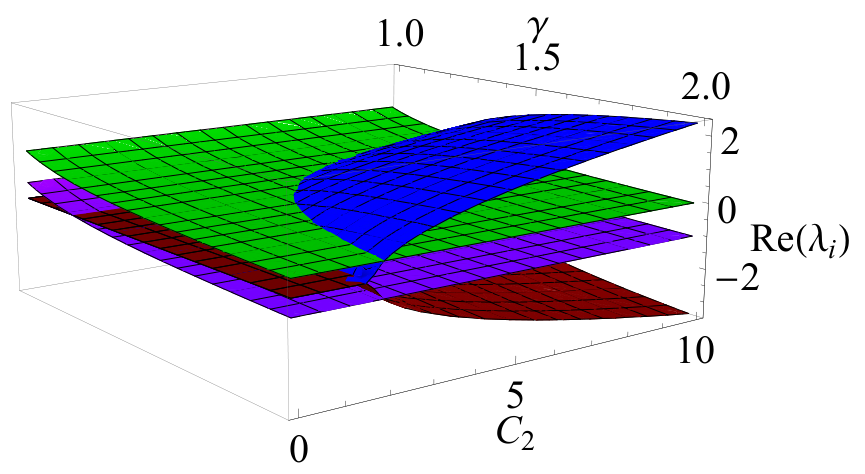
Figure 8: Real part of the eigenvalues for the equilibrium point for y . - (a)
5.6.1 Reduced system
When , the restriction (50) is trivially satisfied. On the other hand, from equation (48) it follows
| (79) |
Imposing the energy condition and choosing , the following reduced dynamical system is obtained:
| (80a) | ||||
| (80b) | ||||
defined in the phase space:
| (81) |
The qualitative analysis of system (80) is given in Table 3.
| Equil. | Eigenvalues (plane –) | Stability (plane –) | ||
| Points | ||||
| saddle | ||||
| saddle for | ||||
| non-hyperbolic for . | ||||
| local source for . | ||||
| local source for . | ||||
| local source for . | ||||
| saddle for . | ||||
| non-hyperbolic for , or | ||||
| . | ||||
| local attractor for | ||||
| . | local attractor for , or | |||
| . | ||||
| non-hyperbolic if . | ||||
| saddle if | . |
| Equil. | Eigenvalues | Stability | |
| Points | |||
| , | non-hyperbolic saddle. | ||
| hyperbolic saddle. | |||
| non-hyperbolic saddle. | |||
| hyperbolic source for . | |||
| hyperbolic saddle for , . | |||
| non-hyperbolic for , or | |||
| . | |||
| hyperbolic saddle . | |||
| hyperbolic sink (see text). | |||
| hyperbolic saddle (see text). | |||
| non-hyperbolic (see text). | |||
| hyperbolic sink for . | |||
| hyperbolic saddle for , or | |||
| , or | |||
| . | |||
| non-hyperbolic for , or | |||
| , or | |||
| . | |||
| non-hyperbolic saddle for . | |||
| non-hyperbolic with three zero eigenvalues for . | |||
| non-hyperbolic with a zero and two purely imaginary eigenvalues | |||
| for . | |||
| if | saddle. | ||
| saddle. | |||
| hyperbolic sink (see text). | |||
| hyperbolic saddle (see text). |
5.7 Summary of sources and sinks for a perfect fluid
A summary of the equilibrium points classified as sinks or sources of the model with perfect fluid is presented.
5.7.1 Non-extensibility surface of solutions
is stable for the regions described in Figure 2.
5.7.2 Invariant sets
- :
, , are hyperbolic sources for .
- :
, , are hyperbolic sources for .
- :
, , is a hyperbolic sink for .
- :
, , is a hyperbolic sink for .
5.7.3 Ideal gas
- :
are hyperbolic sources for
. - :
is hyperbolic sink for .
5.7.4 General case
- :
, are hyperbolic sources for .
- :
, is a hyperbolic sink for:
- (a)
, or
- (b)
.
- (a)
- :
, is a hyperbolic sink for .
- :
, is a hyperbolic sink for:
- (a)
, or
- (b)
, or
- (c)
,
where
. - (a)
5.7.5 Invariant set
- :
, is a hyperbolic source for , .
- :
, is a hyperbolic source for .
Reduced system:
- :
, is a local source for .
- :
is a local source for .
- :
is:
- (a)
a local source for .
- (b)
a local attractor for .
- (a)
- :
is a local sink for:
- (a)
, or
- (b)
.
- (a)
5.8 Discussion
In this section, timelike self-similar spherically symmetric metrics in Einstein-æther theory with perfect fluid as matter content were studied using the homothetic diagonal formulation, which gives the propagation equations (36) plus algebraic restrictions. The homothetic diagonal formalism has some disadvantages. Symmetry surfaces generally change causality. Then, in the homothetic diagonal formulation spacetime must be covered with two coordinate systems (two charts); one when homothetic Killing vector is timelike, and another when homothetic Killing vector is spacelike. These two regions have to be matched in the region where the Killing vector is null Goliath:1998mx. However, the formulation has more advantages than disadvantages. The main one is that it allows the field equations, which are a well-defined system of first-order partial derivative equations (PDE), in two variables (from the formalism), to be written as a system of ordinary differential equations using the symmetries that come from the Killing vectors. The resulting equations are very similar to those of the models with homogeneous hypersurfaces. In turn, it is possible to write these equations as a dynamical system, which makes it possible to study the model using the techniques of the qualitative theory of dynamical systems. This makes it possible to obtain a complete description in a phase space, which leads to a better understanding of the dynamics of the model. In this regard, the –normalized equations were presented.
Four specific models were studied; these are: extreme tilt (61); pressureless perfect fluid (75); the reduced system (80) in the invariant set ; and the general system (78). Hyperbolic points were classified according to their stability conditions using the Hartman-Grobman theorem; while non-hyperbolic points were classified as saddles. Furthermore, it was possible to retrieve the results obtained in Goliath:1998mx. The following list shows the points obtained in Goliath:1998mx and their correspondence with the points discussed in this section:
- :
sonic lines given by , , were analyzed in section 5.1. Unlike General Relativity, for and the system (78) admits the following equilibrium points:
- :
,
- :
,
which lie on the sonic line. If these points exist, and since the fluid behaves like stiff matter. Additionally, if , these points correspond to models with extreme tilt (), , and . corresponds to a flat FLRW space and static orbits depending on the parameter .
- :
- :
, corresponds to .
- :
, correspond to .
- :
, correspond to for .
- :
, correspond to for .
- :
, corresponds to for .
- :
, corresponds to for .
- :
The line , , .
- :
, corresponds to for .
- :
, corresponds to for .
- :
, , corresponds to for .
- :
,
, exists for .
The authors in Goliath:1998mx used the notation , when there is no confusion or is omitted. The kernel indicates the interpretation of the point: represent Minkowski spacetime; represents a Kasner solution; corresponds to static solutions; corresponds to a flat FLRW space and static orbits depending on the parameter ; The equilibrium point line is associated with a change of causality of the homothetic vector field. The points are equilibrium points of (78), only if .
6 Timelike self-similar spherically symmetric models with scalar field
In order for a non-homogeneous scalar field with potential to fulfill the static conformal symmetry they have to have the form Coley:2002je:
where it is assumed, for convenience, , such that for , as .
Then, the energy-momentum tensor of the scalar field is given by:
| (82) |
where denotes the derivative with respect the spatial variable , and:
| (83a) | ||||
| (83b) | ||||
| (83c) | ||||
| (83d) | ||||
The field equations are the following.
Propagation equations:
| (84a) | ||||
| (84b) | ||||
| (84c) | ||||
| (84d) | ||||
| (84e) | ||||
| (84f) | ||||
| (84g) | ||||
Auxiliary equation:
| (85a) | ||||
Restriction:
| (86) |
Equation for :
| (87) |
In general, for , or assuming , the term is dominant, which suggests using -normalized variables.
7 -Normalized equations
The following -normalized variables are introduced:
| (88) |
along with the radial coordinate:
The parameter is defined, analogously to the “Hubble gradient parameter” , by
where
| (89) |
In these variables, the dynamical system is given by:
| (90a) | ||||
| (90b) | ||||
| (90c) | ||||
| (90d) | ||||
| (90e) | ||||
| (90f) | ||||
| (90g) | ||||
The restrictions are:
| (91a) | ||||
| (91b) | ||||
These can be globally resolved for and to get:
| (92a) | ||||
| (92b) | ||||
Finally, the following reduced 5-dimensional system is obtained:
| (93a) | ||||
| (93b) | ||||
| (93c) | ||||
| (93d) | ||||
| (93e) | ||||
If and the limit is taken, system (78) is recovered. Given the computational difficulty of obtaining (analytically) the stability conditions for all the equilibrium points of the system (93), in the following sections some subcases of (93) of special interest will be studied: perfect fluid in the form of ideal gas (97) , the invariant set (99), the extreme tilt case (100) and the invariant set (101). An exhaustive analysis (analytical or numerical) of the stability conditions is provided for these particular cases. Relaxing the condition , interestingly, a cosmological fluid in the form of an ideal gas with equation of state , with describes a FLRW spacetime with non-zero curvature.
7.1 Special case and
The equations are:
| (94a) | ||||
| (94b) | ||||
| (94c) | ||||
| (94d) | ||||
| (94e) | ||||
with restrictions
| (95a) | ||||
| (95b) | ||||
Afterwards, the restrictions are solved to find:
| (96a) | ||||
| (96b) | ||||
Therefore, the following reduced 3-dimensional dynamical system is obtained :
| (97a) | ||||
| (97b) | ||||
| (97c) | ||||

The equilibrium points of the system (97) are the following.
- :
with eigenvalues is a hyperbolic saddle.
- :
, with eigenvalues
,
. It is:- (a)
a hyperbolic sink for:
- i.
, or
- ii.
, or
- iii.
.
- i.
- (b)
and a hyperbolic saddle for:
- i.
, or
- ii.
, or
- iii.
, or
- iv.
, or
- v.
, or
- vi.
, or
- vii.
.
- i.
- (c)
non-hyperbolic for:
- i.
, or
- ii.
.
- i.
- (a)
- :
with eigenvalues
. It exist for , and it is:- (a)
a hyperbolic sink for:
- i.
, or
- ii.
.
- i.
- (b)
a hyperbolic saddle for:
- i.
, or
- ii.
, or
- iii.
, or
- iv.
, or
- v.
.
- i.
- (c)
non-hyperbolic for:
- i.
, or
- ii.
, or
- iii.
, or
- iv.
, or
- v.
.
- i.
- (a)
- :
with eigenvalues
. It is:- (a)
a hyperbolic source for:
- i.
, or
- ii.
.
- i.
- (b)
a hyperbolic saddle for:
- i.
, or
- ii.
, or
- iii.
, or
- iv.
, or
- v.
, or
- vi.
.
- i.
- (c)
non-hyperbolic for:
- i.
, or
- ii.
, or
- iii.
, or
- iv.
, or
- v.
, or
- vi.
.
- i.
- (a)
- :
with eigenvalues
. It is a hyperbolic source for . - :
with eigenvalues . Exists for o . It is:
- (a)
a hyperbolic source for:
- i.
, or
- ii.
.
- i.
- (b)
a hyperbolic saddle for:
- i.
, or
- ii.
.
- i.
- (c)
non-hyperbolic for:
- i.
, or
- ii.
, or
- iii.
, or
- iv.
.
- i.
- (a)
- :
with eigenvalues
where the expressions for depend on . They exist for . In Figure 10, the real parts of the ’s are depicted, so, the equilibrium points are typically saddles or non-hyperbolic with three zero eigenvalues.
7.2 Invariant set
Imposing the following restrictions are deduced:
| (98a) | ||||
| (98b) | ||||
| (98c) | ||||
Finally a reduced dynamical system for the invariant set is obtained
| (99a) | ||||
| (99b) | ||||
| (99c) | ||||
The equilibrium points of system (99) are the following.
- :
has eigenvalues . They are non-hyperbolic saddles for , or, generically, they are saddles because two eigenvalues have opposite signs.
- :
and
- :
with eigenvalues . They are:
- (a)
hyperbolic sources for , or
- (b)
hyperbolic saddles for , or
- (c)
non-hyperbolic for .
- (a)
- :
exists for . The eigenvalues are
. is:- (a)
a hyperbolic sink for
- i.
, or
- ii.
.
- i.
- (b)
a hyperbolic saddle for
- i.
, or
- ii.
.
- i.
- (c)
non-hyperbolic for ,
.
- (a)
- :
exists for . The eigenvalues are
. is:- (a)
a hyperbolic sink for:
- i.
, or
- ii.
,
.
- i.
- (b)
a hyperbolic saddle for:
- i.
, or
- ii.
, or
- iii.
, , or
- iv.
, or
- v.
,
.
- i.
- (c)
non-hyperbolic for:
- i.
, or
- ii.
, or
- iii.
.
- i.
- (a)
- :
exists for . The eigenvalues are
,
. is:- (a)
a hyperbolic sink for:
- i.
, or
- ii.
, or
- iii.
, or
- iv.
, or
- v.
.
- i.
- (b)
a hyperbolic saddle for .
- (c)
non-hyperbolic for:
- i.
, or
- ii.
.
- i.
- (a)
- :
exists for . The eigenvalues are ,
. is:- (a)
a hyperbolic saddle for .
- (b)
non-hyperbolic for .
- (a)
- :
where and
, exists for:- (a)
, or
- (b)
, or
- (c)
o
- (d)
,
.
The eigenvalues are ,
. is:- (a)
a hyperbolic sink for ,
. - (b)
a hyperbolic saddle for:
- i.
, or
- ii.
, or
- iii.
, or
- iv.
.
- i.
- (c)
non-hyperbolic for:
- i.
- ii.
.
- i.
- (a)
- :
where and
, exists for:- (a)
, or
- (b)
, or
- (c)
, or
- (d)
, or
- (e)
,
.
The eigenvalues are ,
. is:- (a)
a hyperbolic sink for:
- i.
, or
- ii.
, or
- iii.
, or
- iv.
,
, or - v.
, or
- vi.
, or
- vii.
where is the real root of , or
- viii.
, where is the real root of , or
- ix.
where is the real root of , or
- x.
.
- i.
- (b)
a hyperbolic saddle for:
- i.
,
, or - ii.
, or
- iii.
, or
- iv.
where is the real root of , or
- v.
,
, or - vi.
, or
- vii.
, or
- viii.
, or
- ix.
.
- i.
- (c)
non-hyperbolic for:
- i.
, or
- ii.
(where is the real root of ), or
- iii.
where is the real root of .
- i.
- (a)
7.3 Invariant sets
Assuming , the system is reduced to the following 4-dimensional dynamical system:
| (100a) | ||||
| (100b) | ||||
| (100c) | ||||
| (100d) | ||||
The equilibrium points of the systems (100) for are the following:
- :
with eigenvalues is a hyperbolic saddle.
- :
with eigenvalues
. This line of equilibrium points contains the equilibrium points studied in section 4. It exists for y . This line is a normally-hyperbolic invariant set. Indeed, the parametric curve can be expressed as:Its tangent vector evaluated at :
is parallel to the eigenvector corresponding to the zero eigevalue:
In this particular case, the stability can be studied considering only the signs of the real parts of the non-zero eigenvalues. In this way it is concluded that:
- (a)
is a hyperbolic source for:
- i.
, or
- ii.
, or
- iii.
,
, or - iv.
,
, or - v.
,
- i.
- (b)
is a hyperbolic saddle for:
- i.
, or
- ii.
,
, or - iii.
,
, or - iv.
,
, or - v.
,
, or - vi.
,
, or - vii.
,
, or - viii.
,
.
- i.
- (c)
is non-hyperbolic for:
- i.
,
, or - ii.
,
, or - iii.
,
, or - iv.
,
, or - v.
,
, or - vi.
,
, or - vii.
,
, or - viii.
,
, or - ix.
,
, or - x.
,
, or - xi.
,
.
- i.
Furthermore,
- (a)
is a hyperbolic source for:
- i.
, or
- ii.
,
, or - iii.
,
.
- i.
- (b)
is a hyperbolic saddle for:
- i.
,
, or - ii.
,
, or - iii.
,
, or - iv.
,
, or - v.
,
, or - vi.
,
.
- i.
- (c)
is non-hyperbolic for
- i.
, or
- ii.
, or
- iii.
,
.
- i.
- (a)
- :
where one eigenvalue is zero and the other three eigenvalues are the roots of the polynomial in :
. It is either a non-hyperbolic saddle or a center depending on the choice of parameters. Figure 11 graphically represents the real part of the corresponding to the equilibrium point , illustrating that the equilibrium points have saddle behavior or they are non-hyperbolic.
Figure 11: Real parts of the ’s corresponding to . - :
with eigenvalues ,
.
It exists for , or .- (a)
is a hyperbolic source for:
- i.
, or
- ii.
.
- i.
- (b)
is a hyperbolic saddle for:
- i.
, or
- ii.
.
- i.
- (c)
is non-hyperbolic for:
- i.
, or
- ii.
, or
- iii.
, or
- iv.
.
- i.
- (a)
- :
with eigenvalues
,
. They are:- (a)
hyperbolic saddles for:
- i.
,
, or - ii.
, or
- iii.
,
, or - iv.
- v.
, or
- vi.
, or
- vii.
,
, or - viii.
, or
- ix.
,
- x.
, .
- i.
- (b)
non-hyperbolic for:
- i.
, or
- ii.
.
- i.
- (a)
- :
with eigenvalues
,
. They are:- (a)
hyperbolic sinks for:
- i.
,
, or - ii.
,
, or - iii.
, .
- i.
- (b)
hyperbolic saddles for:
- i.
,
, or - ii.
, or
- iii.
,
, or - iv.
, or
- v.
, or
- vi.
, or
- vii.
, or
- viii.
,
, or - ix.
,
, or - x.
.
- i.
- (c)
non-hyperbolic for:
- i.
, or
- ii.
.
- i.
- (a)
- :
with eigenvalues ,
,
where . They exist for:
. They are:- (a)
hyperbolic sinks for:
- i.
, or
- ii.
.
- i.
- (b)
hyperbolic saddles for:
- i.
, or
- ii.
, or
- iii.
o,
- iv.
, or
- v.
.
- i.
- (c)
non-hyperbolic for
- i.
, or
- ii.
, or
- iii.
, or
- iv.
.
- i.
- (a)
- :
with eigenvalues ,
,
where . They exist for:
. They are:- (a)
hyperbolic sinks for:
- i.
, or
- ii.
.
- i.
- (b)
hyperbolic saddles for:
- i.
,
, or - ii.
, or
- iii.
, or
- iv.
, or
- v.
,
.
- i.
- (c)
non-hyperbolic for:
- i.
, or
- ii.
, or
- iii.
.
- i.
- (a)
- :
. Exists for or with eigenvalues . In Figure 12 the real parts of are shown, where it can be seen that the point is a hyperbolic saddle or a non-hyperbolic behavior.
Figure 12: Reals parts of corresponding to the equilibrium point . - :
,
. It exists for:- (a)
, or
- (b)
, or
- (c)
.
Figure 13 graphically represents the real part of the eigenvalues of the equilibrium point
, , for different choices of the parameter . This figure illustrates that the point has a general saddle behavior.Figure 13: Real parts of the eigenvalues of the equilibrium point , , for different choices . - (a)
- :
,
with exists for , with eigenvalues
,
. The real parts of ’s are represented in figure 14 (left panel). - :
,
with exists for with eigenvalues
,
. The real parts of the ’s are represented in Figure 14 (right panel). Summarizing, according to Figure 14 these equilibrium points, and , are either sources or they are non-hyperbolic (with four pure imaginary eigenvalues).

Figure 14: Real parts of (left panel) and (right panel) corresponding to the equilibrium points and , respectively. Then, and , are either sources or they are non-hyperbolic (with four pure imaginary eigenvalues).
7.4 Invariant set
At the invariant set , the equations are reduced to:
| (101a) | ||||
| (101b) | ||||
| (101c) | ||||
| (101d) | ||||
| with restriction | ||||
| (101e) | ||||
| For , we have the auxiliary equation: | ||||
| (101f) | ||||
7.4.1 Reduced system
For , the restriction (101e) can be globally solved for , leading to the reduced system:
| (102a) | ||||
| (102b) | ||||
| (102c) | ||||
| (102d) | ||||
For and the system (80) is recovered. Therefore, the equilibrium points, and their stability conditions studied in section 5.6.1 are retrieved. By definition , and (if ). Given that the system (102) is invariant to the simultaneous change , it can be assumed . In the following discussion the analysis is restricted to (the sign of corresponds to the sign of , if ). The following lists contains the equilibrium points of the reduced system (102).
- :
, . The eigenvalues are , then it is a hyperbolic saddle.
- :
, . This line of equilibrium points contains the equilibrium points and studied in section 5.6.1 for . The eigenvalues are . This line is normally-hyperbolic, i. e., given the curve parametrization:
the tangent vector at :
is parallel to the eigenvector associated to the zero eigenvalue, say, In this particular case, the stability of the curve of equilibrium point can be studied considering only the signs of the real part of the non-zero eigenvalues, concluding that:
- (a)
is a hyperbolic source for:
- i.
, or
- ii.
, or
- iii.
,
, or - iv.
,
, or - v.
,
, or - vi.
,
, or - vii.
,
, or - viii.
,
, or - ix.
,
, or - x.
,
, or - xi.
,
, or - xii.
,
, or - xiii.
,
, or - xiv.
,
, or - xv.
,
, or - xvi.
,
.
- i.
- (b)
is a hyperbolic saddle for:
- i.
,
, or - ii.
,
, or - iii.
, or
- iv.
,
, or - v.
,
, or - vi.
, or
- vii.
,
, or - viii.
,
, or - ix.
,
, or - x.
,
, or - xi.
,
, or - xii.
,
, or - xiii.
,
, or - xiv.
,
, or - xv.
,
, or - xvi.
,
, or - xvii.
,
.
- i.
- (c)
is non-hyperbolic for:
- i.
,
, or - ii.
,
, or - iii.
, or
- iv.
, or
- v.
, or
- vi.
,
, or - vii.
,
, or - viii.
,
, or - ix.
,
, or - x.
, or
- xi.
, or
- xii.
,
, or - xiii.
,
, or - xiv.
,
, or - xv.
,
, or - xvi.
,
, or - xvii.
, or
- xviii.
,
, or - xix.
,
, or - xx.
, or
- xxi.
.
- i.
The following list contains new points that were not studied in section 5.6.1.
- (a)
- 1.
.
. The eigenvalues are .- (a)
is a hyperbolic sink for:
- i.
,
, or - ii.
,
, or - iii.
.
- i.
- (b)
is a hyperbolic source for:
- i.
,
, or - ii.
,
.
- i.
- (c)
is non-hyperbolic for:
- i.
, or
- ii.
, or
- iii.
,
, or - iv.
,
, or - v.
, or
- vi.
, or
- vii.
.
- i.
- (d)
is a hyperbolic saddle for:
- i.
, or
- ii.
,
, or - iii.
, or
- iv.
, or
- v.
,
, or - vi.
, or
- vii.
,
, or - viii.
, or
- ix.
, or
- x.
,
, or - xi.
, or
- xii.
,
, or - xiii.
,
, or - xiv.
,
.
- i.
- (a)
- 2.
. . The real parts of the ’s are represented in the figure 15 for some values of , where it is shown that is typically a hyperbolic saddle for the given values of the parameter (or is it non-hyperbolic).


Figure 15: Real parts of the ’s corresponding to for some values of .
The following points are recovered: and .
- 3.
, . The eigenvalues are:
. - 4.
, . The eigenvalues are:
,
. - 5.
, , with eigenvalues
.- (a)
is a hyperbolic sink for:
- i.
, or
- ii.
, or
- iii.
- i.
- (b)
is a hyperbolic source for:
- i.
, or
- ii.
, or
- iii.
.
- i.
- (c)
is non-hyperbolic for:
- i.
, or
- ii.
, or
- iii.
, or
- iv.
, or
- v.
, or
- vi.
, or
- vii.
, or
- viii.
, or
- ix.
, or
- x.
, or
- xi.
, or
- xii.
, or
- xiii.
, or
- xiv.
, or
- xv.
, or
- xvi.
, or
- xvii.
, or
- xviii.
, or
- xix.
, or
- xx.
, or
- xxi.
, or
- xxii.
, or
- xxiii.
, or
- xxiv.
.
- i.
- (d)
is a hyperbolic saddle for:
- i.
,
, or - ii.
,
, or - iii.
,
, or - iv.
, or
- v.
,
, or - vi.
,
, or - vii.
, or
- viii.
,
, or - ix.
,
, or - x.
,
, or - xi.
,
, or - xii.
,
.
- i.
- (a)
7.5 Discussion
In this section, timelike self-similar spherically symmetric models with scalar field (84), were qualitatively analyzed using dynamical systems tools. The first notable feature of the present model is that for non- homogeneous scalar field and its potential to satisfy the homothetic symmetry imposed by the metric, it is required Coley:2002je:
It is assumed that , such that for , as . The equations were normalized with the variable .
Due to the computational complexity of the resulting problem, it was not possible to obtain and analytically treat all the equilibrium points of the system (93). Hence, only some special cases of physical interest were considered, being (97) corresponding to a perfect fluid in the form of an ideal gas, (99) corresponding to the solutions in the invariant set , (100) corresponding to the case of extreme inclination. Finally, the invariant set sets of system (101) was studied. The hyperbolic points were completely classified according to their stability conditions.
8 Conclusions
In this paper the space of the solutions of the differential equations that result from considering perfect fluid and/ or scalar field as the matter content in the Einstein- æther theory was studied. Einstein- æther theory of gravity consists of General Relativity coupled to a vector field of unit time type, called the æther. In this effective theory, the Lorentz invariance is violated, but the locality and the covariance are preserved in the presence of the vector field.
In section 2 the formalism was discussed. This formalism is useful to write the field equations as a system of partial differential equations in two variables for spherically symmetric metrics. Furthermore, using the homothetic diagonal formulation, it was possible to write the partial differential equations as ordinary differential equations using the fact that the metric adapts to homothetic symmetry. The resulting equations (with algebraic restrictions) are very similar to those of the models with homogeneous spatial hypersurfaces Goliath:1998mw. It was then possible to use the techniques of the qualitative theory of dynamical systems for the stability analysis of the solutions of the models. The analytical results were verified by numerical integration.
In the section 3 the Einstein-æther theory of gravity was presented, which contains the theory of General Relativity as a limit. Conformally static metrics were studied in Einstein-æther theory for models of physical interest, such as pressure-free perfect fluids, perfect fluids, and models with extreme tilt. The stability criteria of the equilibrium points of the dynamical systems were obtained and discussed, imposing restrictions on the parameter space. Phase portraits were also presented to illustrate the qualitative behavior of the solutions. The equilibrium points obtained by Goliath:1998mx are recovered as particular cases of the present model. In the notation the kernel indicates the interpretation of the point: represent the Minkowski spacetime; represents a Kasner solution; corresponds to static solutions; corresponds to a flat FLRW space and static orbits depending on the parameter . is associated with a change of causality of the homothetic vector field. The following results were retrieved:
-
: Sonic lines defined by , , were analyzed in section 5.1. As a difference with General Relativity, for and the system (78) admits the following equilibrium points:
- :
,
- :
,
which lie on the sonic line. If these points exist, and since the fluid behaves like stiff matter. Additionally, if , these points correspond to models with extreme tilt (), , and . corresponds to a flat FLRW space and static orbits depending on the parameter .
- :
-
, , exist for . They represent the Minkowski space-time.
-
, corresponds to for . It represents the Minkowski space-time.
-
, corresponds to for . It represents the Minkowski space-time.
-
, corresponds to . It represents the Minkowski space-time.
-
, correspond to . They represent the Minkowski space-time.
-
, corresponds to for . It represents the Kasner solution.
-
, corresponds to for . It represents the Kasner solution.
- 1.
] , correspond to for . They represent the Kasner solution.
-
, correspond to for . They represent the Kasner solution.
-
,
, corresponds to for . - :
The curve of equilibrium points , , . This line of equilibrium points is associated with a change of causality of the homothetic vector field.
These results are of interest in Cosmology and Astrophysics.
In section 6 conformally static metrics were studied in Einstein-æther theory for models with tilted perfect fluid and inhomogeneous scalar field with exponential potential, so the model contains the model studied in section 4 and thus contains the model studied in Goliath:1998mw. Particular cases of interest in Physics were studied, such as the perfect fluid in the form of an ideal gas, solutions with , models with extreme tilt and the invariant set . It was possible to study a more general model than the one studied in Goliath:1998mw, and the results obtained by the authors were reproduced through the use of techniques from the qualitative theory of dynamical systems. A qualitative analysis of some invariant points was also made for models with timelike self-similar spherically symmetric metrics with a perfect fluid and a scalar field. New equilibrium points were obtained, and their stability conditions were found either numerically or analytically, by imposing restrictions on the parameter space.
Acknowledgments G. L. and A. M. acknowledges to Agencia Nacional de Investigación y Desarrollo - ANID for financial support through the program FONDECYT Iniciación grant no. 11180126. Additionally, this research was funded by Vicerrectoría de Investigación y Desarrollo Tecnológico at Universidad Católica del Norte.
References
- [1] Adam G. Riess et al. Observational evidence from supernovae for an accelerating universe and a cosmological constant. Astron. J., 116:1009–1038, 1998.
- [2] P.A.R. Ade et al. Planck 2013 results. I. Overview of products and scientific results. Astron. Astrophys., 571:A1, 2014.
- [3] C.L. Bennett et al. Nine-Year Wilkinson Microwave Anisotropy Probe (WMAP) Observations: Final Maps and Results. Astrophys. J. Suppl., 208:20, 2013.
- [4] P.A.R. Ade et al. Planck 2013 results. XVI. Cosmological parameters. Astron. Astrophys., 571:A16, 2014.
- [5] Adam G. Riess, Lucas Macri, Stefano Casertano, Hubert Lampeitl, Henry C. Ferguson, Alexei V. Filippenko, Saurabh W. Jha, Weidong Li, and Ryan Chornock. A 3% Solution: Determination of the Hubble Constant with the Hubble Space Telescope and Wide Field Camera 3. Astrophys. J., 730:119, 2011. [Erratum: Astrophys.J. 732, 129 (2011)].
- [6] P.A.R. Ade et al. Detection of -Mode Polarization at Degree Angular Scales by BICEP2. Phys. Rev. Lett., 112(24):241101, 2014.
- [7] Jerome Martin. Everything You Always Wanted To Know About The Cosmological Constant Problem (But Were Afraid To Ask). Comptes Rendus Physique, 13:566–665, 2012.
- [8] M. Gasperini. Classical Repulsive Gravity and Broken Lorentz Symmetry. Phys. Rev. D, 34:2260–2262, 1986.
- [9] V.Alan Kostelecky and Stuart Samuel. Phenomenological Gravitational Constraints on Strings and Higher Dimensional Theories. Phys. Rev. Lett., 63:224, 1989.
- [10] Ted Jacobson and David Mattingly. Gravity with a dynamical preferred frame. Phys. Rev. D, 64:024028, 2001.
- [11] Sean M. Carroll and Eugene A. Lim. Lorentz-violating vector fields slow the universe down. Phys. Rev. D, 70:123525, 2004.
- [12] Christopher Eling, Ted Jacobson, and David Mattingly. Einstein-Aether theory. In Deserfest: A Celebration of the Life and Works of Stanley Deser, pages 163–179, 10 2004.
- [13] Eugene A. Lim. Can we see Lorentz-violating vector fields in the CMB? Phys. Rev. D, 71:063504, 2005.
- [14] Sugumi Kanno and Jiro Soda. Lorentz Violating Inflation. Phys. Rev. D, 74:063505, 2006.
- [15] T.G Zlosnik, P.G Ferreira, and G.D Starkman. Modifying gravity with the Aether: An alternative to Dark Matter. Phys. Rev. D, 75:044017, 2007.
- [16] William Donnelly and Ted Jacobson. Coupling the inflaton to an expanding aether. Phys. Rev. D, 82:064032, 2010.
- [17] Isaac Carruthers and Ted Jacobson. Cosmic alignment of the aether. Phys. Rev. D, 83:024034, 2011.
- [18] John D. Barrow. Some Inflationary Einstein-Aether Cosmologies. Phys. Rev. D, 85:047503, 2012.
- [19] Patrik Sandin, Bassemah Alhulaimi, and Alan Coley. Stability of Einstein-Aether Cosmological Models. Phys. Rev. D, 87(4):044031, 2013.
- [20] B. Alhulaimi, A. Coley, and P. Sandin. Anisotropic Einstein-aether cosmological models. J. Math. Phys., 54:042503, 2013.
- [21] Ted Jacobson. Undoing the twist: The Hořava limit of Einstein-aether theory. Phys. Rev. D, 89:081501, 2014.
- [22] Diego Blas and Eugene Lim. Phenomenology of theories of gravity without Lorentz invariance: the preferred frame case. Int. J. Mod. Phys. D, 23:1443009, 2015.
- [23] Alan A. Coley, Genly Leon, Patrik Sandin, and Joey Latta. Spherically symmetric Einstein-aether perfect fluid models. JCAP, 12:010, 2015.
- [24] Joey Latta, Genly Leon, and Andronikos Paliathanasis. Kantowski-Sachs Einstein-æther perfect fluid models. JCAP, 11:051, 2016.
- [25] B. Alhulaimi, R.J. Van Den Hoogen, and A.A. Coley. Spatially homogeneous Einstein-Aether cosmological models: scalar fields with a generalized harmonic potential. JCAP, 12:045, 2017.
- [26] R.J. Van Den Hoogen, A.A. Coley, B. Alhulaimi, S. Mohandas, E. Knighton, and S. O’Neil. Kantowski-Sachs Einstein-Aether Scalar Field Cosmological Models. JCAP, 11:017, 2018.
- [27] Alan Coley and Genly Leon. Static Spherically Symmetric Einstein-aether models I: Perfect fluids with a linear equation of state and scalar fields with an exponential self-interacting potential. Gen. Rel. Grav., 51(9):115, 2019.
- [28] Genly Leon, A. Coley, and Andronikos Paliathanasis. Static spherically symmetric Einstein-æther models II: Integrability and the modified Tolman–Oppenheimer–Volkoff approach. Annals Phys., 412:168002, 2020.
- [29] M. Roumeliotis, A. Paliathanasis, Petros A. Terzis, and T. Christodoulakis. Reduced Lagrangians and analytic solutions in Einstein-æther cosmology. Eur. Phys. J. C, 79(4):349, 2019.
- [30] M. Roumeliotis, A. Paliathanasis, Petros A. Terzis, and T. Christodoulakis. Exact solutions of Einstein-æther gravity in Bianchi type V cosmology. Eur. Phys. J. C, 80(3):239, 2020.
- [31] Andronikos Paliathanasis. Extended analysis for the Evolution of the Cosmological history in Einstein-aether Scalar Field theory. Phys. Rev. D, 101(6):064008, 2020.
- [32] Andronikos Paliathanasis, G. Papagiannopoulos, Spyros Basilakos, and John D. Barrow. Dynamics of Einstein–Aether scalar field cosmology. Eur. Phys. J. C, 79(8):723, 2019.
- [33] Enrico Barausse, Ted Jacobson, and Thomas P. Sotiriou. Black holes in Einstein-aether and Horava-Lifshitz gravity. Phys. Rev. D, 83:124043, 2011.
- [34] William Donnelly and Ted Jacobson. Hamiltonian structure of Horava gravity. Phys. Rev. D, 84:104019, 2011.
- [35] Christopher Eling and Ted Jacobson. Spherical solutions in Einstein-aether theory: Static aether and stars. Class. Quant. Grav., 23:5625–5642, 2006. [Erratum: Class.Quant.Grav. 27, 049801 (2010)].
- [36] Christopher Eling and Ted Jacobson. Black Holes in Einstein-Aether Theory. Class. Quant. Grav., 23:5643–5660, 2006. [Erratum: Class.Quant.Grav. 27, 049802 (2010)].
- [37] Christopher Eling and Ted Jacobson. Two-dimensional gravity with a dynamical aether. Phys. Rev. D, 74:084027, 2006.
- [38] Christopher Eling, Ted Jacobson, and M. Coleman Miller. Neutron stars in Einstein-aether theory. Phys. Rev. D, 76:042003, 2007. [Erratum: Phys.Rev.D 80, 129906 (2009)].
- [39] Joshua W. Elliott, Guy D. Moore, and Horace Stoica. Constraining the new Aether: Gravitational Cerenkov radiation. JHEP, 08:066, 2005.
- [40] Brendan Z. Foster and Ted Jacobson. Post-Newtonian parameters and constraints on Einstein-aether theory. Phys. Rev. D, 73:064015, 2006.
- [41] David Garfinkle, Christopher Eling, and Ted Jacobson. Numerical simulations of gravitational collapse in Einstein-aether theory. Phys. Rev. D, 76:024003, 2007.
- [42] David Garfinkle and Ted Jacobson. A positive energy theorem for Einstein-aether and Hořava gravity. Phys. Rev. Lett., 107:191102, 2011.
- [43] Christian Heinicke, Peter Baekler, and Friedrich W. Hehl. Einstein-aether theory, violation of Lorentz invariance, and metric-affine gravity. Phys. Rev. D, 72:025012, 2005.
- [44] Boris Hikin. Einstein-Aether Theory With and Without Einstein. 3 2010.
- [45] Ted Jacobson. Initial value constraints with tensor matter. Class. Quant. Grav., 28:245011, 2011.
- [46] Ted Jacobson. Extended Horava gravity and Einstein-aether theory. Phys. Rev. D, 81:101502, 2010. [Erratum: Phys.Rev.D 82, 129901 (2010)].
- [47] Ted Jacobson. Einstein-aether gravity: Theory and observational constraints. In 4th Meeting on CPT and Lorentz Symmetry, pages 92–99, 2008.
- [48] Ted Jacobson. Einstein-aether gravity: A Status report. PoS, QG-PH:020, 2007.
- [49] T. Jacobson and D. Mattingly. Einstein-Aether waves. Phys. Rev. D, 70:024003, 2004.
- [50] Ted Jacobson and Antony J. Speranza. Variations on an aethereal theme. Phys. Rev. D, 92:044030, 2015.
- [51] Ted Jacobson and Antony J. Speranza. Comment on ”Scalar Einstein-Aether theory”. 5 2014.
- [52] Masahiro Nakashima and Tsutomu Kobayashi. CMB Polarization in Einstein-Aether Theory. In 20th Workshop on General Relativity and Gravitation in Japan, pages 294–297, 2011.
- [53] Oriol Pujolas and Sergey Sibiryakov. Supersymmetric Aether. JHEP, 01:062, 2012.
- [54] Michael D. Seifert. Stability of spherically symmetric solutions in modified theories of gravity. Phys. Rev. D, 76:064002, 2007.
- [55] Michael D. Seifert and Robert M. Wald. A General variational principle for spherically symmetric perturbations in diffeomorphism covariant theories. Phys. Rev. D, 75:084029, 2007.
- [56] Andronikos Paliathanasis. Inhomogeneous spacetimes in Einstein-æther cosmology. Class. Quant. Grav., 37(10):105008, 2020.
- [57] Supriya Pan, Jaume de Haro, Andronikos Paliathanasis, and Reinoud Jan Slagter. Evolution and Dynamics of a Matter creation model. Mon. Not. Roy. Astron. Soc., 460(2):1445–1456, 2016.
- [58] Baojiu Li and John D. Barrow. Does Bulk Viscosity Create a Viable Unified Dark Matter Model? Phys. Rev. D, 79:103521, 2009.
- [59] Supriya Pan, Barun Kumar Pal, and Souvik Pramanik. Gravitationally influenced particle creation models and late-time cosmic acceleration. Int. J. Geom. Meth. Mod. Phys., 15(03):1850042, 2017.
- [60] Spyros Basilakos, Manolis Plionis, and Joan Solà. Hubble expansion & Structure Formation in Time Varying Vacuum Models. Phys. Rev. D, 80:083511, 2009.
- [61] Spyros Basilakos. Solving the main cosmological puzzles using a modified vacuum energy. Astron. Astrophys., 508:575, 2009.
- [62] Supriya Pan. Exact solutions, finite time singularities and non-singular universe models from a variety of cosmologies. Mod. Phys. Lett. A, 33(01):1850003, 2018.
- [63] V.K. Oikonomou, Supriya Pan, and Rafael C. Nunes. Gravitational Baryogenesis in Running Vacuum models. Int. J. Mod. Phys. A, 32(22):1750129, 2017.
- [64] Genly Leon and Emmanuel N. Saridakis. Phantom dark energy with varying-mass dark matter particles: acceleration and cosmic coincidence problem. Phys. Lett. B, 693:1–10, 2010.
- [65] Andronikos Paliathanasis and Genly Leon. Analytic solutions in Einstein-aether scalar field cosmology. Eur. Phys. J. C, 80(5):355, 2020.
- [66] Andronikos Paliathanasis and Genly Leon. Dynamics and exact Bianchi I spacetimes in Einstein–æther scalar field theory. Eur. Phys. J. C, 80(6):589, 2020.
- [67] Henk van Elst and Claes Uggla. General relativistic (1+3) orthonormal frame approach revisited. Class. Quant. Grav., 14:2673–2695, 1997.
- [68] Martin Goliath, Ulf S. Nilsson, and Claes Uggla. Timelike selfsimilar spherically symmetric perfect fluid models. Class. Quant. Grav., 15:2841, 1998.
- [69] J. Wainwright and G. F. R. Ellis, editors. Dynamical Systems in Cosmology. Cambridge Univ. Press, Cambridge, 1997.
- [70] A. Coley and Y. He. Timelike selfsimilar spherically symmetric models with two scalar fields. Class. Quant. Grav., 19:3901–3925, 2002.
- [71] Hans Stephani, D. Kramer, Malcolm A.H. MacCallum, Cornelius Hoenselaers, and Eduard Herlt. Exact solutions of Einstein’s field equations. Cambridge Monographs on Mathematical Physics. Cambridge Univ. Press, Cambridge, 2003.
- [72] Alan Coley and Sigbjorn Hervik. A Dynamical systems approach to the tilted Bianchi models of solvable type. Class. Quant. Grav., 22:579–606, 2005.
- [73] A.A. Coley, S. Hervik, and W.C. Lim. Fluid observers and tilting cosmology. Class. Quant. Grav., 23:3573–3591, 2006.
- [74] O. I. Bogoyavlensky. Methods in the Qualitative Theory of Dynamical Systems in Astrophysics and Gas Dynamics. Springer Series in Soviet Mathematics. Springer-Verlag, Berlin Heidelberg, 1985.
- [75] Martin Goliath, Ulf S. Nilsson, and Claes Uggla. Spatially selfsimilar spherically symmetric perfect fluid models. Class. Quant. Grav., 15:167, 1998.