Reinforcement Learning in Deep Structured Teams: Initial Results with Finite and Infinite Valued Features
Abstract
In this paper, we consider Markov chain and linear quadratic models for deep structured teams with discounted and time-average cost functions under two non-classical information structures, namely, deep state sharing and no sharing. In deep structured teams, agents are coupled in dynamics and cost functions through deep state, where deep state refers to a set of orthogonal linear regressions of the states. In this article, we consider a homogeneous linear regression for Markov chain models (i.e., empirical distribution of states) and a few orthonormal linear regressions for linear quadratic models (i.e., weighted average of states). Some planning algorithms are developed for the case when the model is known, and some reinforcement learning algorithms are proposed for the case when the model is not known completely. The convergence of two model-free (reinforcement learning) algorithms, one for Markov chain models and one for linear quadratic models, is established. The results are then applied to a smart grid.
Proceedings of IEEE Conference on Control Technology and Applications, 2020. Doi: 10.1109/CCTA41146.2020.9206397.
I Introduction
Recently, there has been a surge of interest in the application of reinforcement learning algorithms in networked control systems such as social networks, swarm robotics, smart grids and transportation networks. This type of systems often consist of many interconnected agents (decision makers) that wish to perform a common task with limited resources in terms of computation, information and knowledge.
When every agent has perfect information and complete knowledge of the entire network, the optimal solution can be computed by dynamic programming decomposition. The computational complexity of solving this dynamic program increases with the number of agents (the so-called “curse of dimensionality”). The above complexity is drastically exacerbated when the information is imperfect. For the case of decentralized information structure with finite spaces, on the other hand, the computational complexity of the resultant dynamic program is NEXP [1], and for infinite spaces with linear quadratic model, the optimization problem is non-convex [2]. In addition, the underlying network model is not always known completely; this lack of knowledge further increases the above complexity. Subsequently, it is very difficult to solve a large-scale control problem with imperfect information of agents and incomplete knowledge of the network.
As an attempt to address the above shortcomings, we propose several reinforcement learning algorithms for a class of multi-agent control problems called deep structured teams, introduced in [3, 4, 5, 6, 7, 8], where the interactions between the decision makers are modelled by a number of linear regressions (weighted averages) of states and actions, which is similar to the interactions between the neurons of a feed-forward deep neural network. In general, deep structured teams are decentralized control systems whose solutions are amenable to the size of the problem. More precisely, the complexity of finding an optimal solution of Markov chain deep structured team is polynomial (rather than exponential) with respect to the number of agents and is linear (rather than exponential) with respect to the control horizon [3]. On the other hand, the complexity of a linear quadratic deep structured team is independent of the number of agents [4]. It is worth highlighting that deep structured teams are the generalization of the notion of mean-field teams initially introduced in [9] and showcased in [10, 11, 12, 13, 14, 15, 16, 17].
The remainder of the paper is organized as follows. In Section II, two models of deep structured teams are formulated, one with finite state and action spaces and the other one with infinite spaces. In Section III, different methods are discussed for solving the planning problem for the case when the model is known. In Section IV, some reinforcement learning methods are presented for the case when the model is not known. An example of a smart grid is provided in Section V to verify the effectiveness of the proposed algorithms, and the paper is then concluded in Section VI.
II Problem Formulation
In this paper, , and are the sets of natural numbers, real numbers and non-negative real numbers, respectively. For any , denotes the finite set and denotes the vector . For any vectors , , and , short-hand notation denotes the vector . For any matrices , and that have the same number of columns, denotes the matrix . Given any square matrices , and , denotes the block diagonal matrix with matrices , and on its main diagonal. In addition, is the probability of a random variable, is the expectation of an event, is the indicator function of a set, is the trace of a matrix, is the infinity norm of a vector, and is the absolute value of a real number or the cardinality of a set. For any , denotes the binomial probability distribution of trials with success probability . For any finite set , the space of probability measures on is denoted by: . Furthermore, the space of empirical distributions over with samples is given by: , where .
Consider a stochastic dynamic control system consisting of agents (decision makers). Let , and denote the state, action and noise of agent at time . In addition, define , , and . The initial states and noises , , are distributed randomly with respect to joint probability distribution functions and , respectively. It is assumed that random variables , , are defined on a common probability space and are mutually independent across any control horizon .
In this paper, we consider two fundamental models in deep structured teams, where the first one has a finite space with a controlled Markov chain formulation and the second one has an infinite space with a linear quadratic structure.
Model I: Finite-valued sets
Let spaces , and be finite sets. Denote by the empirical distribution of states and actions at time , i.e.
| (1) |
Let denote the empirical distribution of states at time :
| (2) |
The agents are coupled in dynamics through , representing the aggregate behaviour of agents at . More precisely, the state of agent at time evolves as follows:
| (3) |
where , and is an i.i.d. random process with probability mass function , i.e., . Alternatively, the dynamics (3) may be written in terms of transition probability matrix:
| (4) |
where .
The agents are also coupled in cost function; this is formulated by defining the per-step cost function at , where and .
Model II: Infinite-valued sets
Let , and be finite-dimensional Euclidean spaces, where . Let also the weight (impact factor) denote the influence of agent on the -th feature, , , where these impact factors are assumed to be orthonormal vectors in the feature space, i.e.,
| (5) |
For feature , define the following linear regressions:
| (6) |
Define and . The dynamics of agent is coupled with other agents through and as follows:
| (7) |
where matrices , , and , , have appropriate dimensions. To have a well-posed problem, it is assumed that the initial states and driving noises have uniformly bounded covariance matrices with respect to time, and that the set of admissible control actions are square integrable for all agents. For simplicity of presentation, it is also assumed that the initial states and local noises have zero mean. The per-step cost function of agent is defined as:
| (8) |
where , , and are symmetric matrices with appropriate dimensions. Let
| (9) | ||||
| (10) | ||||
| (11) |
II-A Information structure
Following the terminology of deep structured teams [3, 4], we refer to the aggregate state of agents as deep state, which is the empirical distribution in Model I and weighted average in Model II. The first information structure considered in this paper is called deep state sharing (DSS). Under this information structure, the action of agent at time in Model I is chosen with respect to a probability mass function , i.e.,
| (Model I: DSS) |
For Model II, however, the action of agent at time is selected with respect to a probability distribution function , i.e.,
| (Model II: DSS) |
In practice, there are various methods to share the deep state among agents. For example, one may use a central distributor (such as a cloud-based server) to collect the states, compute the deep state and broadcast it among the agents. Alternatively, one can utilize distributed techniques such as consensus-based algorithms based on the local interaction of each agent with its neighbours. However, it is sometimes infeasible to share the deep state, specially when the number of agents is very large. In such a case, we consider another information structure called no sharing (NS), where
| (Model I: NS) |
and
| (Model II: NS) |
It is to be noted that the strategy of agent in Model II depends on its index as well as its local state .
II-B Objective function
Let denote the control strategy for the system. Two performance indexes are considered, namely, discounted cost and time-average cost. In particular, given any discount factor , the objective function of Model I is defined as follows:
| (13) |
Similarly, the following discounted cost function is defined for Model II:
| (14) |
In this article, standard mild assumptions are imposed on the model to ensure that the total cost is always bounded. As a result, it is possible to obtain the time-average cost function as the limit of the discounted cost function. More precisely, the following holds for Model I:
| (15) | ||||
| (16) | ||||
| (17) | ||||
| (18) |
Analogously, one has the following for Model II:
| (19) | ||||
| (20) | ||||
| (21) |
It is to be noted that there is no general theory for infinite-space average cost functions.
II-C Problem statement
Four problems are investigated.
Problem 1 (Planning with DSS).
Given dynamics , cost function , number of agents , probability distribution function of the initial states , probability distribution function of noises and discount factor , find the optimal strategy such that under DSS information structure for every strategy :
| (22) |
Problem 2 (Planning with NS).
Given dynamics , cost function , number of agents , probability distribution function of the initial states , probability distribution function of noises and discount factor , find a sub-optimal strategy such that under NS information structure for every strategy :
| (23) |
where .
Problem 3 (Reinforcement learning with DSS).
Given state and action spaces and discount factor , develop a reinforcement learning algorithm whose performance under the learned strategy , , converges to that under the optimal strategy , as the number of iterations increases.
Problem 4 (Reinforcement learning with NS).
Given state and action spaces and discount factor , develop a reinforcement learning algorithm whose performance under the learned strategy , , converges to that under the sub-optimal strategy , as the number of iterations increases.
III Main results for Problems 1 and 2
Following [3], we define a local control law for Model I such that under DSS information structure,
| (24) |
and under NS information structure,
| (25) |
From the definition of DSS and NS strategies given in Subsection II-A and the change of variable introduced in (24) and (25), it follows that the action of agent is selected randomly with respect to the probability mass function , i.e.
| (26) |
Lemma 1.
Given any , and at time , the following relations hold:
| (27) |
and
| (28) |
Proof.
The proof directly follows from (1) such that
| (29) |
where the above equation consists of independent binary random variables with success probability . ∎
To ease the exposition of deep Chapman-Kolmogorov equation introduced in [3], define
| (30) |
Given any , and , define the vector-valued function such that
| (31) |
where is the Dirac measure with the domain set and a unit mass concentrated at zero. In addition, let be the convolution function of over all states , i.e.,
| (32) |
where is a vector of size .
Lemma 2 (Deep Chapman-Kolmogorov equation [3]).
Given and at time , the transition probability matrix of the deep state can be computed as follows: for any and ,
| (33) |
Proof.
We now define a non-standard Bellman equation for Model I such that for every and :
| (34) |
where
| (35) | ||||
| (36) | ||||
| (37) |
Theorem 1.
Proof.
The proof follows from the fact that is an information state under strategy . For more details, see [3, Theorem 2]. ∎
To find the solution of Problem 1 with Model II, we impose the following standard assumption.
Assumption 1.
Let matrices and be positive semi-definite, and matrices and be positive definite. In addition, let and be stabilizable, and and be detectable.
We now describe the algebraic form of the deep Riccati equation introduced in [4, 9]:
| (39) |
Define the following feedback gains:
| (40) |
Remark 2.
For the weakly coupled case in Remark 1, decomposes into smaller Riccati equations such that for any :
| (41) |
where .
Remark 3.
Note that the dimension of the deep Riccati equation (39) does not depend on the number of agents ; however, it depends on the number of orthonormal features .
Theorem 2.
Proof.
The proof follows from a change of variables and certainty equivalence principle. Define
| (44) |
The above change of variables is a gauge transformation, initially introduced in [9] and extended in [4] to optimal control systems and in [5] to dynamic games. From the orthogonality induced by the above gauge transformation, the dynamics (7) and cost function (8) can be decomposed into identical linear quadratic problems with states and actions , , and one linear quadratic problem with state and action . The deep Riccati equation (39) gives the solution of the above problems. For the special case of weakly coupled systems, the Riccati equation associated with the state and action decomposes into smaller Riccati equations given by (41). Note that Assumption 1 implies that for any , and are stabilizable, and and are detectable. As a result, algebraic Riccati equation (39) has a unique, bounded and positive solution. See [4, 9] for more details. ∎
Remark 4 (Extended cost).
The main results of this paper naturally extend to cost functions with post-decision states, i.e., and . In addition, it is straightforward to consider cross terms between the states and actions in (8).
Remark 5 (Generalization).
III-A NS information structure: mean-field approximation
When deep state is not observed, the above solutions are not practical. To overcome this shortcoming, one can approximate the deep state by mean field approximation [19], where the strong law of large numbers provides a simple asymptotic estimate.
Let and denote the mean-field approximations of and , respectively, i.e.,
| (45) |
We now define a non-standard Bellman equation for Model I such that for every and :
| (46) |
where
| (47) | ||||
| (48) |
and for every ,
| (49) |
Assumption 2.
The initial states are i.i.d. random variables with probability mass function .
Assumption 3.
For any , and , there exist positive real constants and (that do not depend on ) such that
| (50) | |||
| (51) |
The above assumption is mild because any polynomial function of is Lipschitz on since is a confined space.
Theorem 3.
Proof.
For Model II, we make the following assumption.
Assumption 4.
For coupled dynamics, an additional stability condition is required to ensure that the proposed infinite-population strategy is stable under NS information structure.
Assumption 5.
Matrix is Hurwitz.
It is to be noted that Assumption 5 holds for decoupled dynamics, where and are zero, . Define mean field such that
| (53) |
where .
Theorem 4.
Proof.
Remark 6.
When the system matrices are independent of the number of agents , the solution of the deep Riccati equation is also independent of for the risk-neutral cost minimization [9, Chapter 3] and minmax optimization [12]. However, this is a rather special case, and more generally, such as in risk-sensitive cost minimization problem [4] and linear quadratic game [5], the solution depends on .
III-B Numerical solutions
To numerically solve the Bellman equations in Theorems 1 and 3, one can quantize the space of probability measures on the local state and local action (i.e. and ), and use standard methods such as value iteration, policy iteration and linear programming, according to [20].
Remark 7.
In practice, value iteration, policy iteration and linear programming suffer from the curse of dimensionality when the size of state and action spaces is large, unless some special structures are imposed such as a linear quadratic model. In Section IV, we discuss more practical approaches that provide more efficient solutions at the cost of losing the optimality. It is worth mentioning that the convergence in policy space is often faster than that in value space.
III-C Decentralized implementation
Model I with DSS
Every agent can independently solve the dynamic program (34) upon the observation of deep state. Since the resultant optimization problem is the same for all agents, the agents commonly choose the control law . Then, agent chooses its action based on its local (private) state and deep state with respect to the probability distribution function at any time (see Theorem 1 for more details).
Model I with NS
For NS information structure, deep state is replaced by mean field, and every agent solves the dynamic program (III-A) by predicting the mean field , given current value and local law , according to (III-A). The resultant performance converges to that of the optimal one as the number of agents goes to infinity; (see Theorem 3 for more details).
Model II with DSS
Every agent solves one Riccati equation of the same order as an individual agent and one Riccati equation whose order is times greater than that of an individual agent given in (39). For the weakly coupled case, every agent solves Riccati equations of an individual agent’s order (Remark 2). Then, each agent computes its action based on its impact factors , local state and deep state (see Theorem 2 for more details).
Model II with NS
For NS information structure, deep state is replaced by mean field and the resultant solution asymptotically converges to the optimal solution as the number of agents goes to infinity.
IV Main results for Problems 3 and 4
In the previous section, it was assumed that the model is completely known. In this section, we provide various techniques to approximate the proposed dynamic programs for the case when the model is not known completely.
In general, there are two fundamental approaches to learning the solution of the proposed dynamic programs. The first one is called model-based approach which uses supervised learning techniques to find the parameters of the models described in Section II, and then solve the planning problems presented in Section III. In short, this approach is an indirect method that obtains the solution by constructing a model. The second approach, however, finds the solution directly without identifying the model. This approach is called reinforcement learning (RL) (also called model-free or approximate dynamic program).
The advantage of the model-based approaches is that they are more intuitional because they not only provide a solution but also construct a model. However, for large-scale problems, it is more efficient to use reinforcement learning methods as they directly search for the solution. In general, there are two types of RL algorithms: off-line and on-line. In the former type, the exploration step is not a major concern as all states and actions can be visited sufficiently often, given a rich set of data and/or simulator. In the latter type, however, it is critical to explore the model in such a way that all states and actions are visited sufficiently often.
IV-A Model I
In what follows, we briefly present the main idea behind approximate value iteration, approximate policy iteration and approximate linear programming. For the approximate value iteration, consider a one-step ahead update of Bellman equation (34) as follows:
| (56) |
where can be approximated as:
| (57) |
such that . In particular, one can use a normalized exponential distribution with the following form:
| (58) |
It is also possible to approximate the value function linearly using feature-based architecture as follows:
| (59) |
Moreover, one can use a multi-step ahead update in (56). Similar function approximations can be used in policy iteration and linear programming. For more details, see [20, 22].
We present Algorithm 1, a (model-free) Q-learning algorithm, wherein attention is restricted to deterministic strategies, i.e., for Model I. Let denote the set of mappings from the local state space to the local action space . It is also possible to use various function approximations to provide a more practical algorithm, albeit at the cost of reduced performance.
| (60) |
Theorem 5.
Suppose that every pair of deep state and local law is visited infinitely often in Algorithm 1. Then, the following results hold:
- (a)
For any , the Q-function converges to with probability one, as .
- (b)
Let be a greedy strategy; then, the performance of converges to that of the optimal strategy given in Theorem 1, when attention is restricted to deterministic strategies.
Proof.
Similar to Theorem 5, one can use a quantized space with quantization level , , similar to the one proposed in [3, Theorem 6], to develop an approximate Q-learning algorithm under NS information structure. The performance of the learned strategy converges to that of Theorem 5 as the number of agents and quantization parameter increase.
Remark 8.
The above results can be extended to stochastic shortest path problem where under the condition that there exists a special cost-free terminal state that absorbs all states under any strategy [24].
IV-B Model II
For Model II, we use a model-free policy-gradient method proposed in [25], and present Algorithm 2. Given a smoothing parameter , let denote the uniform probability distribution over the matrices of size , whose Frobenius norm is . Similarly, let denote the uniform probability distribution over the matrices of size , whose Frobenius norm is .
-
for
- –
initialize states ;
- –
given any agent , use strategy (42) with perturbed feedback gains: and , where and ;
- –
compute the cost trajectories ;
- –
-
end
-
compute and ;
Assumption 6.
The covariance matrices of initial states and driving noises are positive definite (i.e., they are invertible).
Theorem 6.
V Numerical example
The power grid is a complex large-scale network consisting of many decision makers such as users and service providers. Due to some fundamental challenges such as global warming, limited fossil fuel and intermittent nature of renewable energy sources, there is an inevitable need for smart grid wherein the decision makers intelligently interact with each other and use limited resources efficiently. As a result, there has been a growing interest recently in network management of smart grid [26]. In what follows, we provide a simple example showcasing the application of our results in learning the optimal resource allocation strategy.
Example 1. Consider a smart grid with users. Let denote the consumed energy of user at time and denote the weighted average of the total energy consumption of users, i.e.,
| (61) |
where indicates the relative importance (priority) of user compared to others. The linearized dynamics of user is:
| (62) |
where reflects the uncertainty in energy consumption of user at time . The objective is to find a resource allocation strategy such that the following cost is minimized:
| (63) |
where the first two terms are the operational cost of each user and the third term is the cost associated with purchasing energy from a utility.
Suppose that the information structure is deep state sharing, and let all users run Algorithm 2 as their energy management strategy. Consider the following numerical parameters:
| (64) | ||||
| (65) | ||||
| (66) | ||||
| (67) |
where the initial states and local noises are assumed to be i.i.d. random variables.
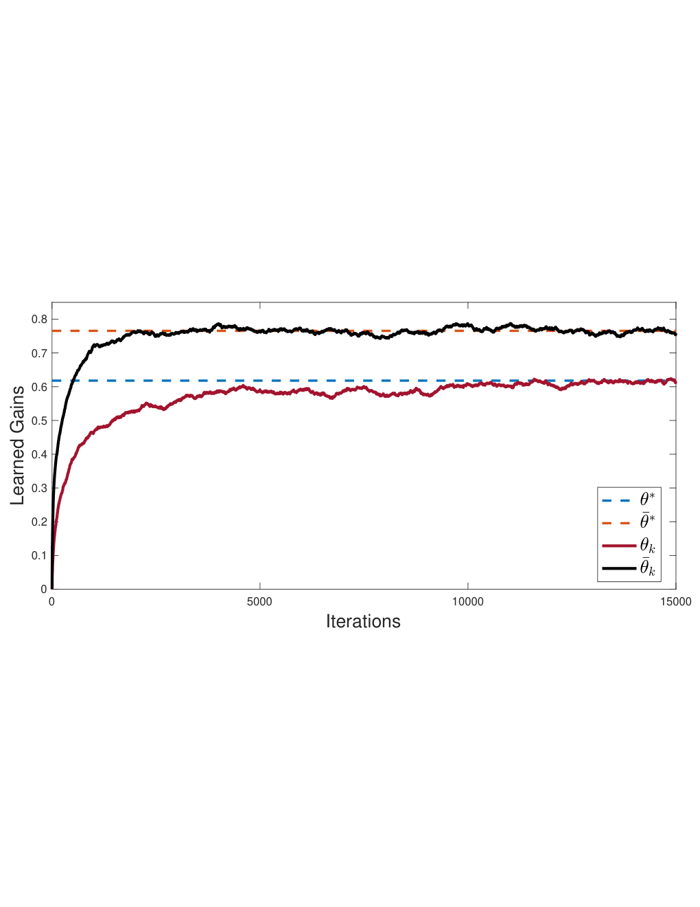
The simulation results are provided in Figure 1, which gives the evolution of learning gains obtained by Algorithm 2 along with the optimal gains. The figure shows that the learned strategy reaches a sufficiently small neighbourhood of the optimal one obtained by Theorem 2, after a few thousand iterations.
VI Conclusions
In this paper, the application of reinforcement learning algorithms in deep structured teams was studied for Markov chain and linear quadratic models with discounted and time-average cost functions. Two non-classical information structures were considered, namely, deep state sharing and no sharing. Different planning and reinforcement leaning algorithms were proposed. In particular, it was shown that the solution of a (model-free) Q-learning algorithm and a (model-free) policy gradient algorithm converge to the optimal solution of the Markov chain model and linear quadratic model, respectively. Finally, the obtained results were applied to smart grid in a simulation environment.
References
- [1] D. S. Bernstein, R. Givan, N. Immerman, and S. Zilberstein, “The complexity of decentralized control of Markov decision processes,” Mathematics of operations research, vol. 27, no. 4, pp. 819–840, 2002.
- [2] H. Witsenhausen, “A counterexample in stochastic optimum control,” SIAM Journal on Control and Opt., vol. 6, pp. 131–147, Dec. 1968.
- [3] J. Arabneydi and A. G. Aghdam, “Deep teams: Decentralized decision making with finite and infinite number of agents,” IEEE Transactions on Automatic Control, vol. 65, no. 10, pp. 4230–4245, 2020.
- [4] ——, “Deep structured teams with linear quadratic model: Partial equivariance and gauge transformation,” [Online]. Available at https://arxiv.org/abs/1912.03951, 2019.
- [5] J. Arabneydi, A. G. Aghdam, and R. P. Malhamé, “Explicit sequential equilibria in LQ deep structured games and weighted mean-field games,” conditionally accepted in Automatica, 2020.
- [6] J. Arabneydi and A. G. Aghdam, “Deep structured teams and games with markov-chain model: Finite and infinite number of players,” Submitted, 2019.
- [7] V. Fathi, J. Arabneydi, and A. G. Aghdam, “Reinforcement learning in linear quadratic deep structured teams: Global convergence of policy gradient methods,” in Proc. of IEEE Conf. on Dec. and Cont., 2020.
- [8] M. Roudneshin, J. Arabneydi, and A. G. Aghdam, “Reinforcement learning in nonzero-sum Linear Quadratic deep structured games: Global convergence of policy optimization,” in Proceedings of the 59th IEEE Conference on Decision and Control, 2020.
- [9] J. Arabneydi, “New concepts in team theory: Mean field teams and reinforcement learning,” Ph.D. dissertation, Dept of Electrical and Computer Engineering, McGill University, Canada, 2016.
- [10] J. Arabneydi and A. G. Aghdam, “A certainty equivalence result in team-optimal control of mean-field coupled Markov chains,” in Proceedings of IEEE Conf. on Dec. and Cont., 2017, pp. 3125–3130.
- [11] M. Baharloo, J. Arabneydi, and A. G. Aghdam, “Near-optimal control strategy in leader-follower networks: A case study for linear quadratic mean-field teams,” in Proceedings of the 57th IEEE Conference on Decision and Control, 2018, pp. 3288–3293.
- [12] ——, “Minmax mean-field team approach for a leader-follower network: A saddle-point strategy,” IEEE Control Systems Letters, vol. 4, no. 1, pp. 121–126, 2019.
- [13] J. Arabneydi, M. Baharloo, and A. G. Aghdam, “Optimal distributed control for leader-follower networks: A scalable design,” in Proceedings of the 31st IEEE Canadian Conference on Electrical and Computer Engineering, 2018, pp. 1–4.
- [14] J. Arabneydi and A. G. Aghdam, “Optimal dynamic pricing for binary demands in smart grids: A fair and privacy-preserving strategy,” in Proceedings of American Control Conference, 2018, pp. 5368–5373.
- [15] J. Arabneydi and A. Mahajan, “Linear quadratic mean field teams: Optimal and approximately optimal decentralized solutions,” Available at https://arxiv.org/abs/1609.00056, 2016.
- [16] ——, “Team-optimal solution of finite number of mean-field coupled LQG subsystems,” in Proceedings of the 54th IEEE Conference on Decision and Control, 2015, pp. 5308 – 5313.
- [17] J. Arabneydi and A. G. Aghdam, “A mean-field team approach to minimize the spread of infection in a network,” in Proceedings of American Control Conference, 2019, pp. 2747–2752.
- [18] ——, “Data collection versus data estimation: A fundamental trade-off in dynamic networks,” IEEE Transactions on Network Science and Engineering, vol. 7, no. 3, pp. 2000–2015, 2020.
- [19] G. Parisi, Statistical field theory. Addison-Wesley, 1988.
- [20] D. P. Bertsekas, Dynamic programming and optimal control. Athena Scientific, 4th Edition, 2012.
- [21] D. A. Bini, B. Iannazzo, and B. Meini, Numerical Solution of Algebraic Riccati Equations. Soc. for Indust. and Appl. Math., 2011.
- [22] R. S. Sutton and A. G. Barto, Reinforcement learning: An introduction. MIT press, 2018.
- [23] J. N. Tsistsiklis, “Asynchronous stochastic approximation and Q-learning,” Machine Learning, vol. 16, pp. 185–202, 1994.
- [24] D. P. Bertsekas and J. N. Tsitsiklis, “An analysis of stochastic shortest path problems,” Mathematics of Operations Research, vol. 16, no. 3, pp. 580–595, 1991.
- [25] M. Fazel, R. Ge, S. M. Kakade, and M. Mesbahi, “Global convergence of policy gradient methods for the linear quadratic regulator,” arXiv preprint arXiv:1801.05039, 2018.
- [26] X. Fang, S. Misra, G. Xue, and D. Yang, “Smart grid—the new and improved power grid: A survey,” IEEE communications surveys & tutorials, vol. 14, no. 4, pp. 944–980, 2012.