“Interpolated Factored Green Function” Method
for accelerated solution of Scattering Problems

Christoph Bauinger Note: Computing and Mathematical Sciences, Caltech, Pasadena, CA 91125, USA Oscar P. Bruno

Abstract

This paper presents a novel Interpolated Factored Green Function method (IFGF) for the accelerated evaluation of the integral operators in scattering theory and other areas. Like existing acceleration methods in these fields, the IFGF algorithm evaluates the action of Green function-based integral operators at a cost of $\mathcal{O}(N\log N)$ operations for an $N$ -point surface mesh. The IFGF strategy, which leads to an extremely simple algorithm, capitalizes on slow variations inherent in a certain Green function analytic factor, which is analytic up to and including infinity, and which therefore allows for accelerated evaluation of fields produced by groups of sources on the basis of a recursive application of classical interpolation methods. Unlike other approaches, the IFGF method does not utilize the Fast Fourier Transform (FFT), and is thus better suited than other methods for efficient parallelization in distributed-memory computer systems. Only a serial implementation of the algorithm is considered in this paper, however, whose efficiency in terms of memory and speed is illustrated by means of a variety of numerical experiments—including a 43 min., single-core operator evaluation (on 10 GB of peak memory), with a relative error of $1.5\times 10^{-2}$ , for a problem of acoustic size of 512 $\lambda$ .

Keywords: Scattering, Green Function, Integral Equations, Acceleration

1 Introduction

This paper presents a new methodology for the accelerated evaluation of the integral operators in scattering theory and other areas. Like existing acceleration methods, the proposed Interpolated Factored Green Function approach (IFGF) can evaluate the action of Green function based integral operators at a cost of $\mathcal{O}(N\log N)$ operations for an $N$ -point surface mesh. Importantly, the proposed method does not utilize previously-employed acceleration elements such as the Fast Fourier transform (FFT), special-function expansions, high-dimensional linear-algebra factorizations, translation operators, equivalent sources, or parabolic scaling [12, 18, 16, 20, 9, 4, 3, 5, 2, 17, 21, 1]. Instead, the IFGF method relies on straightforward interpolation of the operator kernels—or, more precisely, of certain factored forms of the kernels—, which, when collectively applied to larger and larger groups of Green function sources, in a recursive fashion, gives rise to the desired $\mathcal{O}(N\log N)$ accelerated evaluation. The IFGF computing cost is competitive with that of other approaches, and, in a notable advantage, the method runs on a minimal memory footprint. For example, as shown in Table 6 below, a 43-minute, single-core run on a mere 10 GB of peak memory suffice to produce the full discrete operator evaluation, with a relative error of $1.5\times 10^{-2}$ , for a problem 512 wavelengths in acoustic size. In sharp contrast to other algorithms, finally, the IFGF method is extremely simple, and it lends itself to straightforward implementations and effective parallelization.

As alluded to above, the IFGF strategy is based on the interpolation properties of a certain factored form of the scattering Green function into a singular and rapidly-oscillatory centered factor and a slowly-oscillatory analytic factor. Importantly, the analytic factor is analytic up to and including infinity (which enables interpolation over certain unbounded conical domains on the basis of a finite number of radial interpolations nodes), and, when utilized for interpolation of fields with sources contained within a cubic box $B$ of side $H$ , it enables uniform approximability over semi-infinite cones, with apertures proportional to $1/H$ . In particular, unlike the FMM based approaches, the algorithm does not require separate treatment of the low- and high-frequency regimes. On the basis of these properties, the IFGF method orchestrates the accelerated operator evaluation utilizing two separate tree-like hierarchies which are combined in a single boxes-and-cones hierarchical data structure. Thus, starting from an initial cubic box of side $H_{1}$ which contains all source and observation points considered, the algorithm utilizes, like other approaches, the octree $\mathcal{B}$ of boxes that is obtained by partitioning the initial box into eight identical child boxes of side $H_{2}=H_{1}/2$ and iteratively repeating the process with each resulting child box until the resulting boxes are sufficiently small.

Along with the octree of boxes, the IFGF algorithm incorporates a hierarchy $\mathcal{C}$ of cone segments, which are used to enact the required interpolation procedures. Each box in the tree $\mathcal{B}$ is thus endowed with a set of box-centered cone segments at a corresponding level of the cone hierarchy $\mathcal{C}$ . In detail, a set of box-centered cone segments of extent $\Delta_{s,d}$ in the analytic radial variable $s$ , and angular apertures $\Delta_{\theta,d}$ and $\Delta_{\varphi,d}$ in each of the two spherical angular coordinates $\theta$ and $\varphi$ , are used for each $d$ -level box $B$ . (Roughly speaking, $\Delta_{s,d}$ , $\Delta_{\theta,d}$ and $\Delta_{\varphi,d}$ vary in an inversely proportional manner with the box size $H_{d}$ for large enough boxes, but they remain constant for small boxes; full details are presented in Section 3.3.1.) The set of cone segments centered at a box $B$ is used by the IFGF algorithm to set up an interpolation scheme over all of space around $B$ , except for the region occupied by the union of $B$ itself and all of its nearest neighboring boxes at the same level. Thus, the leaves (level $D$ ) in the box tree, that is, the cubes of the smallest size used, are endowed with cone segments of largest angular and radial spans $\Delta_{s,D}$ , $\Delta_{\theta,D}$ and $\Delta_{\varphi,D}$ considered. Each ascent $d\to(d-1)$ by one level in the box tree $\mathcal{B}$ (leading to an increase by a factor of two in the cube side $H_{d-1}=2H_{d}$ ) is accompanied by a corresponding descent by one level (also $d\to(d-1)$ ) in the cone hierarchy $\mathcal{C}$ (leading, e.g., for large boxes, to a decrease by a factor of one-half in the radial and angular cone spans: $\Delta_{s,{d-1}}=\frac{1}{2}\Delta_{s,d}$ , $\Delta_{\theta,{d-1}}=\frac{1}{2}\Delta_{\theta,d}$ and $\Delta_{\varphi,{d-1}}=\frac{1}{2}\Delta_{\varphi,d}$ ; see Section 3.3.1). In view of the interpolation properties of the analytic factor, the interpolation error and cost per point resulting from this conical interpolation setup remains unchanged from one level to the next as the box tree is traversed towards its root level $d=1$ . The situation is even more favorable in the small-box case. And, owing to analyticity at infinity, interpolation for arbitrarily far regions within each cone segment can be achieved on the basis of a finite amount of interpolation data. In all, this strategy reduces the computational cost, by commingling the effect of large numbers of sources into a small number of interpolation parameters. A recursive strategy, in which cone segment interpolation data at level $d$ is also exploited to obtain the corresponding cone-segment interpolation data at level $(d-1)$ , finally, yields the optimal $\mathcal{O}(N\log N)$ approach.

The properties of the factored Green function, which underlie the proposed IFGF algorithm, additionally provide certain perspectives concerning various algorithmic components of other acceleration approaches. In particular, the analyticity properties of the analytic factor, which are established in Theorem 2, in conjunction with the classical polynomial interpolation bound presented in Theorem 1, and the IFGF spherical-coordinate interpolation strategy, clearly imply the property of low-rank approximability which underlies some of the ideas associated with the butterfly [16, 18, 7] and directional FMM methods [12]. The directional FMM approach, further, relies on a “directional factorization” which, in the context of the present interpolation-based viewpoint, can be interpreted as facilitating interpolation. For the directional factorization to produce beneficial effects it is necessary for the differences of source and observation points to lie on a line asymptotically parallel to the vector between the centers of the source and target boxes. This requirement is satisfied in the directional FMM approach through its “parabolic-scaling”, according to which the distance to the observation set is required to be the square of the size of the source box. The IFGF factorization is not directional, however, and it does not require use of the parabolic scaling: the IFGF approach interpolates analytic-factor contributions at linearly-growing distances from the source box.

In a related context we mention the recently introduced approach [3], which incorporates in an ${\mathcal{H}}^{2}$ -matrix setting some of the main ideas associated with the directional FMM algorithm [12]. Like the IFGF method, the approach relies on interpolation of a factored form of the Green function—but using the directional factorization instead of the IFGF factorization. The method yields a full LU decomposition of the discrete integral operator, but it does so under significant computing costs and memory requirements, both for pre-computation, and per individual solution.

It is also useful to compare the IFGF approach to other acceleration methods from a purely algorithmic point of view. The FMM-based approaches [12, 4, 9, 15] entail two passes over the three-dimensional acceleration tree, one in the upward direction, the other one downward. In the upward pass of the original FMM methods, for example, the algorithm commingles contributions from larger and larger numbers of sources via correspondingly growing spherical harmonics expansions, which are sequentially translated to certain spherical coordinate systems and then recombined, as the algorithm progresses up the tree via application of a sequence of so-called M2M translation operators (see e.g. [12]). In the downward FMM pass, the algorithm then re-translates and localizes the spherical-harmonic expansions to smaller and smaller boxes via related M2L and L2L translation operators (e.g. [12]). The algorithm is finally completed by evaluation of surface point values at the end of the downward pass. The IFGF algorithm, in contrast, progresses simultaneously along two tree-like structures, the box tree and the cone interpolation hierarchy, and it produces evaluations at the required observation points, via interpolation, at all stages of the acceleration process (but only in a neighborhood of each source box at each stage). In particular, the IFGF method does not utilize high-order expansions of the kinds used in other acceleration methods—and, thus, it avoids use of Fast Fourier Transforms (FFTs) which are almost invariably utilized in the FMM to manipulate the necessary spherical harmonics expansions. (Reference [14, Sec. 7] mentions two alternatives which, however, it discards as less efficient than an FFT-based procedure.) The use of FFTs presents significant challenges, however, in the context of distributed memory parallel computer systems. In this regard reference [12] (further referencing [21]), for example, indicates “the top part of the [FMM] octree is a bottleneck” for parallelization, and notes that, in view of the required parabolic scaling, the difficulty is not as marked for the directional FMM approach proposed in that contribution. In [8] the part of the FMM relying on FFTs is identified to become a bottleneck in the parallelization and it is stated that this difficulty occurs as the FFT-based portion of the algorithm is subject to the “lowest arithmetic intensity” and is therefore “likely suffering from bandwidth contention”.

The IFGF algorithm, which relies on interpolation by means of Chebyshev expansions of relatively low degree, does not require the use of FFTs—a fact that, as suggested above, provides significant benefits in the distributed memory context. As a counterpoint, however, the low degree Chebyshev approximations used by the IFGF method do not yield the spectral accuracy resulting from the high-order expansions used by other methods. A version of the IFGF method which enjoys spectral accuracy could be obtained simply by replacing its use of low-order Chebyshev interpolation by Chebyshev interpolation of higher and higher orders on cone segments of fixed size as the hierarchies are traversed toward the root $d=1$ . Such a direct approach, however, entails a computing cost which increases quadratically as the Chebyshev expansion order grows—thus degrading the optimal complexity of the IFGF method. But the needed evaluation of high-order Chebyshev expansions on arbitrary three-dimensional grids can be performed by means of FFT-based interpolation methods similar to those utilized in [5, Sec. 3.1] and [6, Remark 7]. This approach, which is not pursued in this paper, leads to a spectrally convergent version of the method, which still runs on essentially linear computing time and memory. But, as it reverts to use of FFTs, the strategy re-introduces the aforementioned disadvantages concerning parallelization, which are avoided in the proposed IFGF approach.

It is also relevant to contrast the algorithmic aspects in the IFGF approach to those used in the butterfly approaches [18, 16, 7]. Unlike the interpolation-based IFGF, which does not rely on use of linear-algebra factorizations, the butterfly approaches are based on low rank factorizations of various high-dimensional sub-matrices of the overall system matrix. Certain recent versions of the butterfly methods reduce linear-algebra computational cost by means of an interpolation process in high-dimensional space in a process which can easily be justified on the basis of the analytic properties of the factored Green function described in Section 3.1. As in the IFGF approach, further, the data structure inherent in the butterfly approach [18, 16] is organized on the basis of two separate tree structures that are traversed in opposite directions, one ascending and the other descending, as the algorithm progresses. In the method [18] the source and observation cubes are paired in such a way that the product their sizes remains constant—which evokes the IFGF’s cone-and-box sizing condition, according to which the angles scale inversely with the cone span angles. These two selection criteria are indeed related, as the interpolability by polynomials used in the IFGF approach has direct implications on the rank of the interpolated values. But, in a significant distinction, the IFGF method can be applied to a wide range of scattering kernels, including the Maxwell, Helmholtz, Laplace and elasticity kernels among others, and including smooth as well as non-smooth kernels. The butterfly approaches [7, 18], in contrast, only apply to Fourier integral operators with smooth kernels. The earlier butterfly contribution [16] does apply to Maxwell problems, but its accuracy, specially in the low-frequency near-singular interaction regime, has not been studied in detail.

Whereas no discussion concerning parallel implementation of the IFGF approach is presented in this paper, we note that, not relying on FFTs, the approach is not subject to the challenging FFT communication requirements inherent in all of the aforementioned Maxwell/Helmholtz/Laplace algorithms. In fact, experience in the case of the butterfly method [18] for non-singular kernels, whose data structure is, as mentioned above, similar to the one utilized in the IFGF method, suggests that efficient parallelization to large numbers of processors may hold for the IFGF algorithm as well. In [18] this was achieved due to “careful manipulation of bitwise-partitions of the product space of the source and target domains” to “keep the data (…) and the computation (…) evenly distributed”.

This paper is organized as follows: after preliminaries are briefly considered in Section 2, Section 3 presents the details of the IFGF algorithm—including, in Sections 3.1 and 3.2, a theoretical discussion of the analyticity and interpolation properties of the analytic factor, and then, in Section 3.3, the algorithm itself. The numerical results presented in Section 4 demonstrate the efficiency of the IFGF algorithm in terms of memory and computing costs by means of several numerical experiments performed on different geometries with acoustic size up to 512 wavelengths. A few concluding comments, finally, are presented in Section 5.

2 Preliminaries and Notation

We consider discrete integral operators of the form

I(x_{\ell})\coloneqq\sum\limits_{\begin{subarray}{c}m=1\\ m\neq\ell\end{subarray}}^{N}a_{m}G(x_{\ell},x_{m}),\quad\ell=1,\ldots,N,

(1)

on a two-dimensional surface $\Gamma\subset\mathbb{R}^{3}$ , where $N$ denotes a given positive integer, and where, for $m=1,\ldots,N$ , $x_{m}\in\Gamma$ and $a_{m}\in\mathbb{C}$ denote pairwise different points and given complex numbers, respectively; the set of all $N$ surface discretization points, in turn, is denoted by $\Gamma_{N}\coloneqq\{x_{1},\ldots,x_{N}\}$ . For definiteness, throughout this paper we focus mostly on the challenging three-dimensional Helmholtz Green function case,

G(x,x^{\prime})=\frac{e^{\imath\kappa|x-x^{\prime}|}}{4\pi|x-x^{\prime}|},

(2)

where $\imath$ , $\kappa$ and $|\cdot|$ denote the imaginary unit, the wavenumber and the Euclidean norm in $\mathbb{R}^{3}$ , respectively. Discrete operators of the form (1), with various kernels $G$ , play major roles in a wide range of areas in science and engineering, with applications to acoustic and electromagnetic scattering by surfaces and volumetric domains in two- and three-dimensional space, potential theory, fluid flow, etc. As illustrated in Section 3.2 for the Laplace kernel $G(x,x^{\prime})=1/|x-x^{\prime}|$ , the proposed acceleration methodology applies, with minimal variations, to a wide range of smooth and non-smooth kernels—including but not limited to, e.g. the Laplace, Stokes and elasticity kernels, and even kernels of the form $G(x,x^{\prime})=\exp{\left(\imath\varphi(x-x^{\prime})\right)}$ for smooth functions $\varphi$ . The restriction to surface problems, where the point sources lie on a two dimensional surface $\Gamma$ in three dimensional space, is similarly adopted for definiteness: the extension of the method to volumetric source distributions is straightforward and should prove equally effective.

Clearly, a direct evaluation of $I(x)$ for all $x\in\Gamma_{N}$ requires $\mathcal{O}(N^{2})$ operations. This quadratic algorithmic complexity makes a direct operator evaluation unfeasible for many problems of practical interest. In order to accelerate the evaluation, the proposed IFGF method partitions the surface points $\Gamma_{N}$ by means of a hierarchical tree structure of boxes, as described in Section 3.3. The evaluation of the operator (1) is then performed on basis of a small number of pairwise box interactions, which may occur either horizontally in the tree structure, between two nearby equi-sized boxes, or vertically between a child box and a neighboring parent-level box. As shown in Section 3, the box interactions can be significantly accelerated by means of a certain interpolation strategy that is a centerpiece in the IFGF approach. The aforementioned box tree, together with an associated cone structure, are described in detail in Section 3.3.

To conclude this section we introduce the box, source-point and target-point notations we use in what follows. To do this, for given $H>0$ and $x=((x)_{1},(x)_{2},(x)_{3})^{T}\in\mathbb{R}^{3}$ we define the axis aligned box $B(x,H)$ of box side $H$ and centered at $x$ as

B(x,H)\coloneqq\left[(x)_{1}-\frac{H}{2},(x)_{1}+\frac{H}{2}\right)\times\left[(x)_{2}-\frac{H}{2},(x)_{2}+\frac{H}{2}\right)\times\left[(x)_{3}-\frac{H}{2},(x)_{3}+\frac{H}{2}\right);

(3)

see Figure 1. For a given source box $B(x_{S},H)$ of side $H$ and centered at a given point $x_{S}=\left((x_{S})_{1},(x_{S})_{2},(x_{S})_{3}\right)^{T}\in\mathbb{R}^{3}$ , we use the enumeration $x_{1}^{S},\ldots,x_{N_{S}}^{S}\in B(x_{S},H)\cap\Gamma_{N}$ ( $N_{S}\leq N$ and, possibly, $N_{S}=0$ ) of all source points $x_{m}$ , $m=1,\dots,N$ , which are contained in $B(x_{S},H)$ ; the corresponding source coefficients $a_{m}$ are denoted by $a_{\ell}^{S}\in\{a_{1},\ldots,a_{N}\}$ , $\ell=1,\ldots,N_{S}$ . A given set of $N_{T}$ surface target points, at arbitrary positions outside $B(x_{S},H)$ , are denoted by $x_{1}^{T},\ldots,x_{N_{T}}^{T}\in\Gamma_{N}\setminus B(x_{S},H)$ . Then, letting $I_{S}=I_{S}(x)$ denote the field generated at a point $x$ by all point sources contained in $B(x_{S},H)$ , we will consider, in particular, the problem of evaluation of the local operator

I_{S}(x_{\ell}^{T})\coloneqq\sum\limits_{m=1}^{N_{S}}a_{m}^{S}G(x_{\ell}^{T},x_{m}^{S}),\qquad\ell=1,\ldots,N_{T}.

(4)

A sketch of this setup is presented in Figure 1.

Refer to caption — Figure 1: Two-dimensional illustration of a source box $B(x_{S},H)$ containing source points $x_{1}^{S},x_{2}^{S},x_{3}^{S},\ldots$ (blue circles) and target points $x_{1}^{T},x_{2}^{T},x_{3}^{T},\ldots$ (green stars). The black wavy lines represent the field $I_{S}$ generated by the point sources in $B(x_{S},H)$ .

3 The IFGF Method

To achieve the desired acceleration of the discrete operator (1), the IFGF approach utilizes a certain factorization of the Green function $G$ which leads to efficient evaluation of the field $I_{S}$ in equation (4) by means of numerical methods based on polynomial interpolation.

The IFGF factorization for $x^{\prime}$ in the box $B(x_{S},H)$ (centered at $x_{S}$ ) takes the form

G(x,x^{\prime})=G(x,x_{S})g_{S}(x,x^{\prime}).

(5)

Throughout this paper the functions $G(x,x_{S})$ and $g_{S}$ are called the centered factor and the analytic factor, respectively. Clearly, for a fixed given center $x_{S}$ the centered factor depends only on $x$ : it is independent of $x^{\prime}$ . As shown in Section 3.1, in turn, the analytic factor is analytic up to and including infinity in the $x$ variable for each fixed value of $x^{\prime}$ (which, in particular, makes $g_{S}(x,x^{\prime})$ slowly oscillatory and asymptotically constant as a function of $x$ as $|x|\to\infty$ ), with oscillations as a function of $x$ that, for $x^{\prime}\in B(x_{S},H)$ , increase linearly with the box size $H$ .

Using the factorization (5) the field $I_{S}$ generated by point sources placed within the source box $B(x_{S},H)$ at any point $x\in\mathbb{R}^{3}$ may be expressed in the form

I_{S}(x)=\sum\limits_{m=1}^{N_{S}}a_{m}^{S}G(x,x_{m}^{S})=G(x,x_{S})F_{S}(x)\quad\mbox{where}\quad F_{S}(x)=\sum\limits_{m=1}^{N_{S}}a_{m}^{S}g_{S}(x,x_{m}^{S}).

(6)

The desired IFGF accelerated evaluation of the operator (4) is achieved via interpolation of the function $F_{S}(x)$ , which, as a linear combination of analytic factors, is itself analytic at infinity. The singular and oscillatory character of the function $F_{S}$ , which determine the cost required for its accurate interpolation, can be characterized in terms of the analytic properties, mentioned above, of the factor $g_{S}$ . A study of these analytic and interpolation properties is presented in Sections 3.1 and 3.2.

On the basis of the aforementioned analytic properties the algorithm evaluates all the sums in equation (4) by first obtaining values of the function $F_{S}$ at a small number $P\in\mathbb{N}$ of points $p_{i}\in\mathbb{R}^{3}$ , $i=1,\ldots,P$ , from which the necessary $I_{S}$ values (at all the target points $x_{1}^{T},\ldots,x_{N_{T}}^{T}$ ) are rapidly and accurately obtained by interpolation. At a cost of $\mathcal{O}(PN_{S}+PN_{T})$ operations, the interpolation-based algorithm yields useful acceleration provided $P\ll\min\{N_{S},N_{T}\}$ . Section 3.3 shows that adequate utilization of these elementary ideas leads to a multi-level algorithm which applies the forward map (1) for general surfaces at a total cost of $\mathcal{O}(N\log N)$ operations. The algorithm (which is very simple indeed) and a study of its computational cost are presented in Section 3.3.

In order to proceed with this program we introduce certain notations and conventions. On one hand, for notational simplicity, but without loss of generality, throughout the remainder of this section we assume $x_{S}=0$ ; the extension to the general $x_{S}\neq 0$ case is, of course, straightforward. Incorporating the convention $x_{S}=0$ , then, we additionally consider, for $0<\eta<1$ , the sets

A_{\eta}\coloneqq\{(x,x^{\prime})\in\mathbb{R}^{3}\times\mathbb{R}^{3}\,:\,|x^{\prime}|\leq\eta|x|\}

and

A_{\eta}^{H}\coloneqq A_{\eta}\cap\left(\mathbb{R}^{3}\times B(x_{S},H)\right).

(7)

Clearly, $A_{\eta}^{H}$ is the subset of pairs in $A_{\eta}$ such that $x^{\prime}$ is restricted to a particular source box $B(x_{S},H)$ . Theorem 2 below implies that, on the basis of an appropriate change of variables which adequately accounts for the analyticity of the function $g_{S}$ up to and including infinity, this function can be accurately evaluated for $(x,x^{\prime})\in A_{\eta}^{H}$ by means of a straightforward interpolation rule based on an interpolation mesh in spherical coordinates which is very sparse along the radial direction.

3.1 Analyticity

As indicated above, the analytic properties of the factor $g_{S}$ play a pivotal role in the proposed algorithm. Under the $x_{S}=0$ convention established above, the factors in equation (5) become

G(x,0)=\frac{e^{\imath\kappa|x|}}{4\pi|x|}\quad\mbox{and}\quad g_{S}(x,x^{\prime})=\frac{|x|}{|x-x^{\prime}|}e^{\imath\kappa\left(|x-x^{\prime}|-|x|\right)}.

(8)

In order to analyze the properties of the factor $g_{S}$ we introduce the spherical coordinate parametrization

\tilde{\mathbf{x}}(r,\theta,\varphi)\coloneqq\begin{pmatrix}r\sin\theta\cos\varphi\\ r\sin\theta\sin\varphi\\ r\cos\theta\end{pmatrix},\qquad 0\leq r<\infty,\mkern 5.0mu0\leq\theta\leq\pi,\mkern 5.0mu0\leq\varphi<2\pi,

(9)

and note that (8) may be re-expressed in the form

g_{S}(x,x^{\prime})=\frac{1}{4\pi\left|\frac{x}{r}-\frac{x^{\prime}}{r}\right|}\exp\left({\imath\kappa r\left(\left|\frac{x}{r}-\frac{x^{\prime}}{r}\right|-1\right)}\right).

(10)

The effectiveness of the proposed factorization is illustrated in Figures 2(a), 2(b), and 2(c), where the oscillatory character of the analytic factor $g_{S}$ and the Green function (2) without factorization are compared, as a function of $r$ , for several wavenumbers. The slowly-oscillatory character of the factor $g_{S}$ , even for acoustically large source boxes $B(x_{S},H)$ as large as twenty wavelengths $\lambda$ ( $H=20\lambda$ ) and starting as close as just $3H/2$ away from the center of the source box, is clearly visible in Figure 2(c); much faster oscillations are observed in Figure 2(b), even for source boxes as small as two wavelengths in size ( $H=2\lambda$ ). Only the real part is depicted in Figures 2(a), 2(b), and 2(c) but, clearly, the imaginary part displays the same behavior.

While the oscillations of the smooth factor $g_{S}$ and the unfactored Green function are asymptotically the same for an increasing acoustic size of the source box ( $\kappa H\to\infty$ , cf. Theorem 2), a strategy based on direct interpolation of the Green function without factorization of the complex exponential term would require several orders of magnitudes more interpolation points and proportional computational effort. While allowing that the cost of such an approach may be prohibitive, it is interesting to note that, asymptotically, the cost would still be of the order of $\mathcal{O}(N\log N)$ operations.

In addition to the factorization (6), the proposed strategy relies on use of the singularity resolving change of variables

{\color[rgb]{0,0,0}s\coloneqq\frac{h}{r},\qquad{\mathbf{x}}(s,\theta,\varphi)\coloneqq\tilde{\mathbf{x}}(r,\theta,\varphi),}

(11)

where, once again, $r=|x|$ denotes the radius in spherical coordinates and where $h$ denotes the radius of the source box—which is related to the box size $H$ by

h\coloneqq\max\limits_{x\in B(x_{S},H)}|x|=\frac{\sqrt{3}}{2}H.

(12)

Using these notations equation (10) may be re-expressed in the form

g_{S}(x,x^{\prime})=\frac{1}{4\pi\left|\frac{x}{r}-\frac{x^{\prime}}{h}s\right|}\exp\left({\imath\kappa r\left(\left|\frac{x}{r}-\frac{x^{\prime}}{h}s\right|-1\right)}\right).

(13)

Note that while the source point $x$ and its norm $r$ depend on $s$ , the quantity $x/r$ is independent of $r$ and therefore also of $s$ .

The introduction of the variable $s$ gives rise to several algorithmic advantages, all of which stem from the analyticity properties of the function $g_{S}$ —as presented in Lemma 1 below and Theorem 2 in Section 3.2. Briefly, these results establish that, for any fixed values $H>0$ and $\eta$ satisfying $0<\eta<1$ , the function $g_{S}$ is analytic for $(x,x^{\prime})\in A_{\eta}^{H}$ , with $x$ -derivatives that are bounded up to and including $|x|=\infty$ . As a result (as shown in Section 3.2) the $s$ change of variables translates the problem of interpolation of $g_{S}$ over an infinite $r$ interval into a problem of interpolation of an analytic function of the variable $s$ over a compact interval in the $s$ variable.

The relevant $H$ -dependent analyticity domains for the function $g_{S}$ for each fixed value of $H$ are described in the following lemma.

Lemma 1.

Let $x^{\prime}\in B(x_{S},H)$ and let $x_{0}=\tilde{\mathbf{x}}(r_{0},\theta_{0},\varphi_{0})=\mathbf{x}(s_{0},\theta_{0},\varphi_{0})$ ( $s_{0}=h/r_{0}$ ) be such that $(x_{0},x^{\prime})\in A_{\eta}^{H}$ . Then $g_{S}$ is an analytic function of $x$ around $x_{0}$ and also an analytic function of $(s,\theta,\varphi)$ around $(s_{0},\theta_{0},\varphi_{0})$ . Further, the function $g_{S}$ is an analytic function of $(s,\theta,\varphi)$ (resp. $(r,\theta,\varphi)$ ) for $0\leq\theta\leq\pi$ , $0\leq\varphi<2\pi$ , and for $s$ in a neighborhood of $s_{0}=0$ (resp. for $r$ in a neighborhood of $r_{0}=\infty$ , including $r=r_{0}=\infty$ ).

Proof.

The claimed analyticity of the function $g_{S}$ around $x_{0}=\mathbf{x}(s_{0},\theta_{0},\varphi_{0})$ (and, thus, the analyticity of $g_{S}$ around $(s_{0},\theta_{0},\varphi_{0})$ ) is immediate since, under the assumed hypothesis, the quantity

\left|\frac{x}{r}-\frac{x^{\prime}}{h}s\right|,

(14)

does not vanish in a neighborhood of $x=x_{0}$ . Analyticity around $s_{0}=0$ ( $r_{0}=\infty$ ) follows similarly since the quantity (14) does not vanish around $s=s_{0}=0$ . ∎

Corollary 1.

Let $H>0$ be given. Then for all $x^{\prime}\in B(x_{S},H)$ the function $g_{S}({\mathbf{x}}(s,\theta,\varphi),x^{\prime})$ is an analytic function of $(s,\theta,\varphi)$ for $0\leq s<1$ , $0\leq\theta\leq\pi$ and $0\leq\varphi<2\pi$ .

Proof.

Take $\eta\in(0,1)$ . Then, for $0\leq s\leq\eta$ we have $({\mathbf{x}}(s,\theta,\varphi),x^{\prime})\in A_{\eta}^{H}$ . The analyticity for $0\leq s\leq\eta$ follows from Lemma 1, and since $\eta\in(0,1)$ is arbitrary, the lemma follows. ∎

For a given $x^{\prime}\in\mathbb{R}^{3}$ , Corollary 1 reduces the problem of interpolation of the function $g_{S}(x,x^{\prime})$ in the $x$ variable to a problem of interpolation of a re-parametrized form of the function $g_{S}$ over a bounded domain—provided that $(x,x^{\prime})\in A_{\eta}^{H}$ , or, in other words, provided that $x$ is separated from $x^{\prime}$ by a factor of at least $\eta$ , for some $\eta<1$ . In the IFGF algorithm presented in Section 3.3, side- $H$ boxes $B(x_{S},H)$ containing sources $x^{\prime}$ are considered, with target points $x$ at a distance no less than $H$ away from $B(x_{S},H)$ . Clearly, a point $(x,x^{\prime})$ in such a configuration necessarily belongs to $A_{\eta}^{H}$ with $\eta=\sqrt{3}/3$ . Importantly, as demonstrated in the following section, the interpolation quality of the algorithm does not degrade as source boxes of increasingly large side $H$ are used, as is done in the proposed multi-level IFGF algorithm (with a single box size at each level), leading to a computing cost per level which is independent of the level box size $H$ .

3.2 Interpolation

On the basis of the discussion presented in Section 3.1, the present section concerns the problem of interpolation of the function $g_{S}$ in the variables $(s,\theta,\varphi)$ . For efficiency, piece-wise Chebyshev interpolation in each one of these variables is used, over interpolation intervals of respective lengths $\Delta_{s}$ , $\Delta_{\theta}$ and $\Delta_{\varphi}$ , where, for a certain positive integer $n_{C}$ , angular coordinate intervals of size

\Delta_{\theta}=\Delta_{\varphi}=\frac{\pi}{n_{C}},

are utilized. Defining

\theta_{k}=k\Delta_{\theta},\quad(k=0,\ldots,n_{C}-1)\quad\mbox{and}\quad\varphi_{\ell}=\ell\Delta_{\varphi},\quad(\ell=0,\ldots,2n_{C}-1),

as well as

E^{\varphi}_{j}=[\varphi_{j-1},\varphi_{j})\quad\text{ and }\quad E^{\theta}_{i,j}=\begin{cases}[\theta_{n_{C}-1},\pi]\quad&\text{for}\quad i=n_{C},\mkern 5.0muj=2n_{C}\\ (0,\Delta_{\theta})\quad&\text{for}\quad i=1,\mkern 5.0muj>1\\ [\theta_{i-1},\theta_{i})\quad&\text{otherwise,}\end{cases}

(15)

we thus obtain the mutually disjoint interpolation cones

\tilde{C}_{i,j}\coloneqq\left\{x=\tilde{\mathbf{x}}(r,\theta,\varphi)\,:\,r\in(0,\infty),\mkern 5.0mu\theta\in E^{\theta}_{i,j},\mkern 5.0mu\varphi\in E^{\varphi}_{j}\right\},\quad(i=1,\dots,n_{C},j=1,\ldots,2n_{C}),

(16)

centered at $x_{S}=(0,0,0)^{T}$ . Note that the definition (16) ensures that

\bigcup\limits_{\begin{subarray}{c}1=1,\ldots,n_{C}\\ j=1,\ldots,2n_{C}\end{subarray}}\tilde{C}_{i,j}=\mathbb{R}^{3}\setminus\{0\}\qquad\text{and}\qquad\tilde{C}_{i,j}\cap\tilde{C}_{k,l}=\emptyset\quad\text{for}\quad(i,j)\neq(k,l).

The proposed interpolation strategy additionally relies on a number $n_{s}\in\mathbb{N}$ of disjoint radial interpolation intervals $E_{k}^{s}$ , $k=1,\ldots,n_{s}$ , of size $\Delta_{s}=\eta/n_{s}$ , within the IFGF $s$ -variable radial interpolation domain $[0,\eta]$ (with $\eta=\sqrt{3}/3$ , see Section 3.1). Thus, in all, the approach utilizes an overall number $N_{C}\coloneqq n_{s}\times n_{C}\times 2n_{C}$ of interpolation domains

E_{\gamma}\coloneqq E_{\gamma_{1}}^{s}\times E_{\gamma_{2}}^{\theta}\times E_{\gamma_{3}}^{\varphi},

(17)

which we call cone domains, with $\mathbf{\gamma}=(\gamma_{1},\gamma_{2},\gamma_{3})\in\{1,\ldots,n_{s}\}\times\{1,\ldots,n_{C}\}\times\{1,\ldots,2n_{C}\}$ . Under the parametrization $\mathbf{x}$ in equation (11), the cone domains yield the cone segment sets

C_{\mathbf{\gamma}}\coloneqq\{x=\mathbf{x}(s,\theta,\varphi)\,:\,(s,\theta,\varphi)\in E_{\gamma}\}.

(18)

Note that, by definition, the cone segments are mutually disjoint. A two-dimensional illustration of the cone domains and associated cone segments is provided in Figure 3.

The desired interpolation strategy then relies on the use of a fixed number $P=P_{\text{ang}}^{2}P_{\text{s}}$ of interpolation points for each cone segment $C_{\mathbf{\gamma}}$ , where $P_{\text{ang}}$ (resp. $P_{\text{s}}$ ) denotes the number of Chebyshev interpolation points per interval used for each angular variable (resp. for the radial variable $s$ ). For each cone segment, the proposed interpolation approach proceeds by breaking up the problem into a sequence of one-dimensional Chebyshev interpolation problems of accuracy orders $P_{s}$ and $P_{\text{ang}}$ , as described in [19, Sec. 3.6.1], along each one of the three coordinate directions $s$ , $\theta$ and $\varphi$ . This spherical Chebyshev interpolation procedure is described in what follows, and an associated error estimate is presented which is then used to guide the selection of cone segment sizes.

The one-dimensional Chebyshev interpolation polynomial $I^{\mathrm{ref}}_{n}u$ of accuracy order $n$ for a given function $u:[-1,1]\to\mathbb{C}$ over the reference interval $[-1,1]$ is given by the expression

I^{\mathrm{ref}}_{n}u(x)=\sum\limits_{i=0}^{n-1}a_{i}T_{i}(x),\quad x\in[-1,1],

(19)

where $T_{i}(x)=\cos(i\arccos(x))$ denotes the $i$ -th Chebyshev polynomial of the first kind, and where, letting

x_{k}=\cos\left(\frac{2k+1}{2n}\pi\right),\quad b_{i}=\left\{\begin{array}[]{ll}1&i\neq 0\\ 2&i=0,\end{array}\right.\quad\mbox{and}\quad c_{k}=\left\{\begin{array}[]{ll}0.5&k=0\text{ or }k=n-1\\ 1&\text{else},\end{array}\right.

the coefficients $a_{i}\in\mathbb{C}$ are given by

a_{i}=\frac{2}{b_{i}(n-1)}\sum\limits_{k=0}^{n-1}c_{k}u(x_{k})T_{i}(x_{k}).

(20)

Chebyshev expansions for functions defined on arbitrary intervals $[a,b]$ result from use of a linear interval mapping to the reference interval $[-1,1]$ ; for notational simplicity, the corresponding Chebyshev interpolant in the interval $[a,b]$ is denoted by $I_{n}u$ , without explicit reference to the interpolation interval $[a,b]$ .

As is known ([10, Sec. 7.1], [13]), the one-dimensional Chebyshev interpolation error $|u(x)-I_{n}u(x)|$ in the interval $[a,b]$ satisfies the bound

|u(x)-I_{n}u(x)|\leq\frac{(b-a)^{n}}{2^{2n-1}n!}\left\lVert\frac{\partial^{n}u}{\partial x^{n}}\right\rVert_{\infty},

(21)

where

\left\lVert\frac{\partial^{n}u}{\partial x^{n}}\right\rVert_{\infty}\coloneqq\sup\limits_{c\in(a,b)}\left|\frac{\partial^{n}u}{\partial x^{n}}(c)\right|

(22)

denotes the supremum norm of the $n$ -th partial derivative. The desired error estimate for the nested Chebyshev interpolation procedure within a cone segment (18) (or, more precisely, within the cone domains (17)) is provided by the following theorem.

Theorem 1.

Let $I_{P_{s}}^{s}$ , $I_{P_{\text{ang}}}^{\theta}$ , and $I_{P_{\text{ang}}}^{\varphi}$ denote the Chebyshev interpolation operators of accuracy orders $P_{s}$ in the variable $s$ and $P_{\text{ang}}$ in the angular variables $\theta$ and $\varphi$ , over intervals $E^{s}$ , $E^{\theta}$ , and $E^{\varphi}$ of lengths $\Delta_{s}$ , $\Delta_{\theta}$ , and $\Delta_{\varphi}$ in the variables $s$ , $\theta$ , and $\varphi$ , respectively. Then, for each arbitrary but fixed point $x^{\prime}\in\mathbb{R}^{3}$ the error arising from nested interpolation of the function $g_{S}(\mathbf{x}(s,\theta,\varphi),x^{\prime})$ (cf. equation (11)) in the variables $(s,\theta,\varphi)$ satisfies the estimate

|g_{S}(\mathbf{x}(s,\theta,\varphi),x^{\prime})-I_{P_{\text{ang}}}^{\varphi}I_{P_{\text{ang}}}^{\theta}I_{P_{s}}^{s}g_{S}(\mathbf{x}(s,\theta,\varphi),x^{\prime})|\leq\\ C\left[(\Delta_{s})^{P_{\text{s}}}\left\lVert\frac{\partial^{P_{s}}g_{S}}{\partial s^{P_{s}}}\right\rVert_{\infty}+(\Delta_{\theta})^{P_{\text{ang}}}\left\lVert\frac{\partial^{P_{\text{ang}}}g_{S}}{\partial\theta^{P_{\text{ang}}}}\right\rVert_{\infty}+(\Delta_{\varphi})^{P_{\text{ang}}}\left\lVert\frac{\partial^{P_{\text{ang}}}g_{S}}{\partial\varphi^{P_{\text{ang}}}}\right\rVert_{\infty}\right],

(23)

for some constant $C$ depending only on $P_{s}$ and $P_{\text{ang}}$ , where the supremum-norm expressions are shorthands for the supremum norm defined by

\left\lVert\frac{\partial^{n}g_{S}}{\partial\xi^{n}}\right\rVert_{\infty}\coloneqq\sup\limits_{\begin{subarray}{c}\tilde{s}\in E^{s}\\ \tilde{\theta}\in E^{\theta}\\ \tilde{\varphi}\in E^{\varphi}\end{subarray}}\left|\frac{\partial^{n}g_{S}}{\partial\xi^{n}}({\mathbf{x}}(\tilde{s},\tilde{\theta},\tilde{\varphi}),x^{\prime})\right|

for $\xi=s$ , $\theta$ , or $\varphi$ .

Proof.

The proof is only presented for a double-nested interpolation procedure; the extension to the triple-nested method is entirely analogous. Suppressing, for readability, the explicit functional dependence on the variables $x$ and $x^{\prime}$ , use of the triangle inequality and the error estimate (21) yields

	$\displaystyle\|g_{S}-I_{P_{\text{ang}}}^{\theta}I_{P_{s}}^{s}g_{S}\|$	$\displaystyle\leq\|f-I_{P_{s}}^{s}g_{S}\|+\|I_{P_{\text{ang}}}^{\theta}I_{P_{s}}^{s}g_{S}-I_{P_{s}}^{s}g_{S}\|$
		$\displaystyle\leq C_{1}(\Delta_{s})^{P_{s}}\left\lVert\frac{\partial^{P_{s}}g_{S}}{\partial s^{P_{s}}}\right\rVert_{\infty}+C_{2}(\Delta_{\theta})^{P_{\text{ang}}}\left\lVert\frac{\partial^{P_{\text{ang}}}I_{P_{s}}^{s}g_{S}}{\partial\theta^{P_{\text{ang}}}}\right\rVert_{\infty},$

where $C_{1}$ and $C_{2}$ are constants depending on $P_{s}$ and $P_{\text{ang}}$ , respectively. In order to estimate the second term on the right-hand side in terms of derivatives of $g_{S}$ we utilize equation (20) in the shifted arguments corresponding to the $s$ -interpolation interval $(a,b)$ :

I_{P_{s}}^{s}g_{S}=\sum\limits_{i=0}^{P_{s}-1}a_{i}^{s}(\theta)T_{i}\left(2\frac{s-a}{b-a}-1\right),\quad(b=a+\Delta_{s}).

Differentiation with respect to $\theta$ and use of the relations (19) and (20) then yield

\left\lVert\frac{\partial^{P_{\text{ang}}}I_{P_{s}}^{s}g_{S}}{\partial\theta^{P_{\text{ang}}}}\right\rVert_{\infty}\leq P_{s}\max\limits_{i=1,\ldots,P_{s}-1}\left\lVert\frac{\partial^{P_{\text{ang}}}a_{i}^{s}}{\partial\theta^{P_{\text{ang}}}}\right\rVert_{\infty}\leq C_{3}\left\lVert\frac{\partial^{P_{\text{ang}}}g_{S}}{\partial\theta^{P_{\text{ang}}}}\right\rVert_{\infty},

as it may be checked, for a certain constant $C_{3}$ depending on $P_{s}$ , by employing the triangle inequality and the $L^{\infty}$ bound $\left\lVert T_{i}\right\rVert_{\infty}\leq 1$ ( $i\in\mathrm{\mathbb{N}_{0}=\mathbb{N}\cup\{0\}}$ ). The more general error estimate (23) follows by a direct extension of this argument to the triple-nested case, and the proof is thus complete. ∎

The analysis presented in what follows, including Lemmas 2 through 4 and Theorem 2, yields bounds for the partial derivatives in (23) in terms of the acoustic size $\kappa H$ of the source box $B(x_{S},H)$ . Subsequently, these bounds are used, together with the error estimate (23), to determine suitable choices of the cone domain sizes $\Delta_{s}$ , $\Delta_{\theta}$ , and $\Delta_{\varphi}$ , ensuring that the errors resulting from the triple-nested interpolation process lie below a prescribed error tolerance. Leading to Theorem 2, the next three lemmas provide estimates, in terms of the box size $H$ , of the $n$ -th order derivatives ( $n\in\mathbb{N}$ ) of certain functions related to $g_{S}(\mathbf{x}(s,\theta,\varphi),x^{\prime})$ , with respect to each one of the variables $s$ , $\theta$ , and $\varphi$ and every $x^{\prime}\in B(x_{S},H)$ .

Lemma 2.

Under the change of variables $x={\mathbf{x}}(s,\theta,\varphi)$ in (11), for all $n\in\mathbb{N}$ and for either $\xi=\theta$ or $\xi=\varphi$ , we have

\frac{\partial^{n}}{\partial\xi^{n}}|x-x^{\prime}|=\sum\frac{c(m_{1},\ldots,m_{n})}{|x-x^{\prime}|^{2k-1}}\prod\limits_{j=1}^{n}\left\langle\frac{\partial^{j}x}{\partial\xi^{j}},x^{\prime}\right\rangle^{m_{j}},

where the outer sum is taken over all $n$ -tuples $(m_{1},\ldots,m_{n})\in\mathbb{N}_{0}^{n}$ such that

\sum\limits_{j=1}^{n}jm_{j}=n,

where $k:=\sum_{i=1}^{n}m_{i}$ , where $c(m_{1},\ldots,m_{n})\in\mathbb{R}$ denote constants independent of $x$ , $x^{\prime}$ and $\xi$ , and where $\langle\cdot,\cdot\rangle$ denotes the Euclidean inner product on $\mathbb{R}^{3}$ .

Proof.

The proof follows from Faà di Bruno’s formula [11] applied to $f(g(x))=|x-x^{\prime}|$ , where $f(x)=\sqrt{x}$ and $g(x)=\langle x,x\rangle-2\langle x,x^{\prime}\rangle+\langle x^{\prime},x^{\prime}\rangle$ . Indeed, noting that

\frac{d^{k}f(x)}{dx^{k}}=c_{1}(k)\frac{1}{f(x)^{2k-1}},

for some constant $c_{1}(k)$ , and that, since $\langle\frac{\partial x}{\partial\xi},x\rangle=0$ for $\xi=\theta$ and $\xi=\varphi$ ,

\frac{\partial^{i}g(x(\xi))}{d\xi^{i}}=c_{2}(i)\left\langle\frac{\partial^{i}x}{\partial\xi^{i}},x^{\prime}\right\rangle,

for some constant $c_{2}(i)$ , an application of Faà di Bruno’s formula directly yields the desired result. ∎

Lemma 3.

Let $H>0$ and $\eta\in(0,1)$ be given. Then, under the change of variables $x={\mathbf{x}}(s,\theta,\varphi)$ in (11), the exponent in the right-hand exponential in (8) satisfies

\frac{\partial^{n}}{\partial\xi^{n}}\left(|x-x^{\prime}|-|x|\right)\leq C(\eta,n)H,

for all $(x,x^{\prime})\in A_{\eta}^{H}$ , for all $n\in\mathbb{N}_{0}$ , and for $\xi=s$ , $\xi=\theta$ and $\xi=\varphi$ , where $C(\eta,n)$ is a certain real constant that depends on $\eta$ and $n$ , but which is independent of $H$ .

Proof.

Expressing the exponent in (8) in terms of $s$ yields

\displaystyle|x-x^{\prime}|-|x|=\frac{h}{s}\left(\left|\frac{x}{r}-\frac{x^{\prime}}{h}s\right|-1\right)=:hg(s),

(24)

where our standing assumption $x_{S}=0$ and notation $|x|=r$ have been used (so that, in particular, $x/r$ is independent of $r$ and therefore also independent of $s$ ), and where the angular dependence of the function $g$ has been suppressed. Clearly, $g(s)$ is an analytic function of $s$ for $s\in\big[0,h/|x^{\prime}|\big)$ and, thus, since $\eta<1$ , for $s$ in the compact interval $\big[0,\eta\cdot h/|x^{\prime}|\big]$ . It follows that $g$ and each one of its derivatives with respect to $s$ is uniformly bounded for all $s\in\big[0,\eta\cdot h/|x^{\prime}|\big]$ and (as shown by a simple re-examination of the discussion above) for all $H$ and for all values of $x/r$ and $x^{\prime}/h$ under consideration. Since at the point $(x,x^{\prime})$ we have $s=h/|x|=|x^{\prime}|/|x||\cdot h/|x^{\prime}\leq\eta\cdot h/|x^{\prime}|$ , using (12) once again, the desired $\xi=s$ estimate

\frac{\partial^{n}}{\partial s^{n}}\left(hg(s)\right)\leq C(\eta,n)H,

follows, for some constant $C(\eta,n)$ .

Turning to the angular variables, we only consider the case $\xi=\theta$ ; the case $\xi=\varphi$ can be treated similarly. Using Lemma 2 for $\xi=\theta$ , the Cauchy Schwarz inequality and the assumption $(x,x^{\prime})\in A_{\eta}^{H}$ , we obtain

	$\displaystyle\left\|\frac{\partial^{n}\left(\|x-x^{\prime}\|-\|x\|\right)}{\partial\theta^{n}}\right\|$	$\displaystyle=\left\|\frac{\partial^{n}\left(\|x-x^{\prime}\|\right)}{\partial\theta^{n}}\right\|=\left\|\sum\frac{c(m_{1},\ldots,m_{n})}{\|x-x^{\prime}\|^{2k-1}}\prod\limits_{j=1}^{n}\left\langle\frac{\partial^{j}x}{\partial\xi^{j}},x^{\prime}\right\rangle^{m_{j}}\right\|$
		$\displaystyle\leq\sum\frac{\|c(m_{1},\ldots,m_{n})\|}{\|x-x^{\prime}\|^{2k-1}}\prod\limits_{j=1}^{n}\left\|\frac{\partial^{j}x}{\partial\xi^{j}}\right\|^{m_{j}}\left\|x^{\prime}\right\|^{m_{j}}\leq\sum\limits_{k=1}^{n}\hat{C}(\eta,n)\frac{1}{r^{2k-1}}r^{k}\left\|x^{\prime}\right\|^{k}$
		$\displaystyle\leq\tilde{C}(\eta,n)\left\|x^{\prime}\right\|\leq C(\eta,n)H,$

where the same notation as in Lemma 2 was used. The constant $C(\eta,n)$ has been suitably adjusted. The proof is now complete. ∎

Lemma 4.

Let $H>0$ and $\eta\in(0,1)$ be given. Then, under the change of variables $x={\mathbf{x}}(s,\theta,\varphi)$ in (11), for all $(x,x^{\prime})\in A_{\eta}^{H}$ , for all $n\in\mathbb{N}_{0}$ , and for $\xi=s$ , $\xi=\theta$ and $\xi=\varphi$ , we have

\left|\frac{\partial^{n}}{\partial\xi^{n}}e^{\imath\kappa\left(|x-x^{\prime}|-|x|\right)}\right|\leq\tilde{M}(\eta,n)\left(\kappa H\right)^{n},

where $\tilde{M}(\eta,n)$ is a certain real constant that depends on $\eta$ and $n$ but which is independent of $H$ .

Proof.

Using Faà di Bruno’s formula [11] yields

\frac{\partial^{n}}{\partial\xi^{n}}e^{\imath\kappa\left(|x-x^{\prime}|-|x|\right)}=\sum c(m_{1},\ldots,m_{n})e^{\imath\kappa\left(|x-x^{\prime}|-|x|\right)}\prod\limits_{j=1}^{n}\left(\imath\kappa\frac{\partial^{j}\left(|x-x^{\prime}|-|x|\right)}{\partial\xi^{j}}\right)^{m_{j}},

where the sum is taken over all $n$ -tuples $(m_{1},\ldots,m_{n})\in\mathbb{N}_{0}^{n}$ such that

\sum\limits_{j=1}^{n}jm_{j}=n,

and where $c(m_{1},\ldots,m_{n})$ are certain constants which depend on $m_{1},\ldots,m_{n}$ . Using the triangle inequality and Lemma 3 then completes the proof. ∎

The desired bounds on derivatives of the function $g_{S}$ are presented in the following theorem.

Theorem 2.

\left|\frac{\partial^{n}g_{S}}{\partial\xi^{n}}\right|\leq M(\eta,n)\max{\left\{(\kappa H)^{n},1\right\}},

where $M(\eta,n)$ is a certain real constant that depends on $\eta$ and $n$ but which is independent of $H$ .

Proof.

The quotient on the right-hand side of (8) may be re-expressed in the form

\displaystyle\frac{|x|}{|x-x^{\prime}|}=\frac{1}{\left|\frac{x}{r}-\frac{x^{\prime}}{h}s\right|},

(25)

where $x/r$ is independent of $r$ and therefore also independent of $s$ . An analyticity argument similar to the one used in the proof of Lemma 3 shows that this quotient, as well as each one of its derivatives with respect to $s$ , is uniformly bounded for $s$ throughout the interval $\big[0,\eta\cdot h/|x^{\prime}|\big]$ , for all $H>0$ , and for all relevant values of $x/r$ and $x^{\prime}/h$ .

In order to obtain the desired estimates we now utilize Leibniz’ differentiation rule, which yields

\displaystyle\left|\frac{\partial^{n}g_{S}(x,x^{\prime})}{\partial\xi^{n}}\right|=\left|\sum\limits_{i=0}^{n}\binom{n}{i}\frac{\partial^{n-i}}{\partial\xi^{n-i}}\left(\frac{|x|}{|x-x^{\prime}|}\right)\frac{\partial^{i}}{\partial\xi^{i}}\left(e^{\imath\kappa\left(|x-x^{\prime}|-|x|\right)}\right)\right|\leq C(\eta,n)\sum\limits_{i=0}^{n}\frac{\partial^{i}}{\partial\xi^{i}}e^{\imath\kappa\left(|x-x^{\prime}|-|x|\right)},

for some constant $C(\eta,n)$ that depends on $\eta$ and $n$ , but which is independent of $H$ . Applying Lemma 4 and suitably adjusting constants the result follows. ∎

In view of the bound (23), Theorem 2 shows that the interpolation error remains uniformly small provided that the interpolation interval sizes $\Delta_{s}$ , $\Delta_{\theta}$ , and $\Delta_{\varphi}$ are held constant for $\kappa H<1$ and are taken to decrease like $\mathcal{O}(1/(\kappa H))$ as the box sizes $\kappa H$ grow when $\kappa H\geq 1$ .

This observation motivates the main strategy in the IFGF algorithm. As the algorithm progresses from one level to the next, the box sizes are doubled, from $H$ to $2H$ , and the cone segment interpolation interval lengths $\Delta_{s}$ , $\Delta_{\theta}$ , and $\Delta_{\varphi}$ are either kept constant or decreased by a factor of $1/2$ (depending on whether $\kappa H<1$ or $\kappa H\geq 1$ , respectively)—while the interpolation error, at a fixed number of degrees of freedom per cone segment, remains uniformly bounded. The resulting hierarchy of boxes and cone segments is embodied in two different but inter-related hierarchical structures: the box octree and a hierarchy of cone segments. In the box octree each box contains eight equi-sized child boxes. In the cone segment hierarchy, similarly, each cone segment (spanning certain angular and radial intervals) spawns up to eight child segments. The $\kappa H\to\infty$ limit then is approached as the box tree structure is traversed from children to parents and the accompanying cone segment structure is traversed from parents to children. This hierarchical strategy and associated structures are described in detail in Section 3.3.

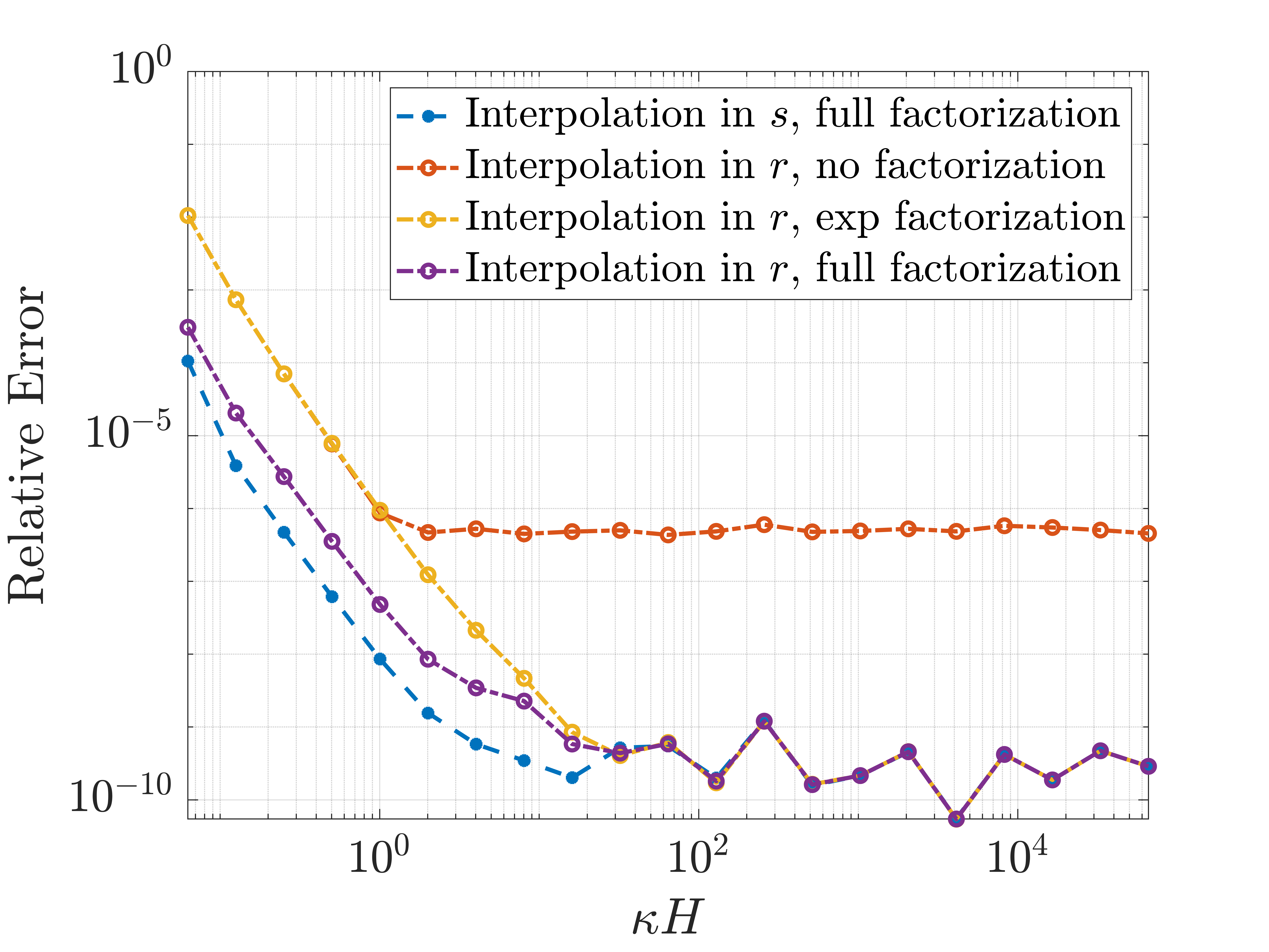
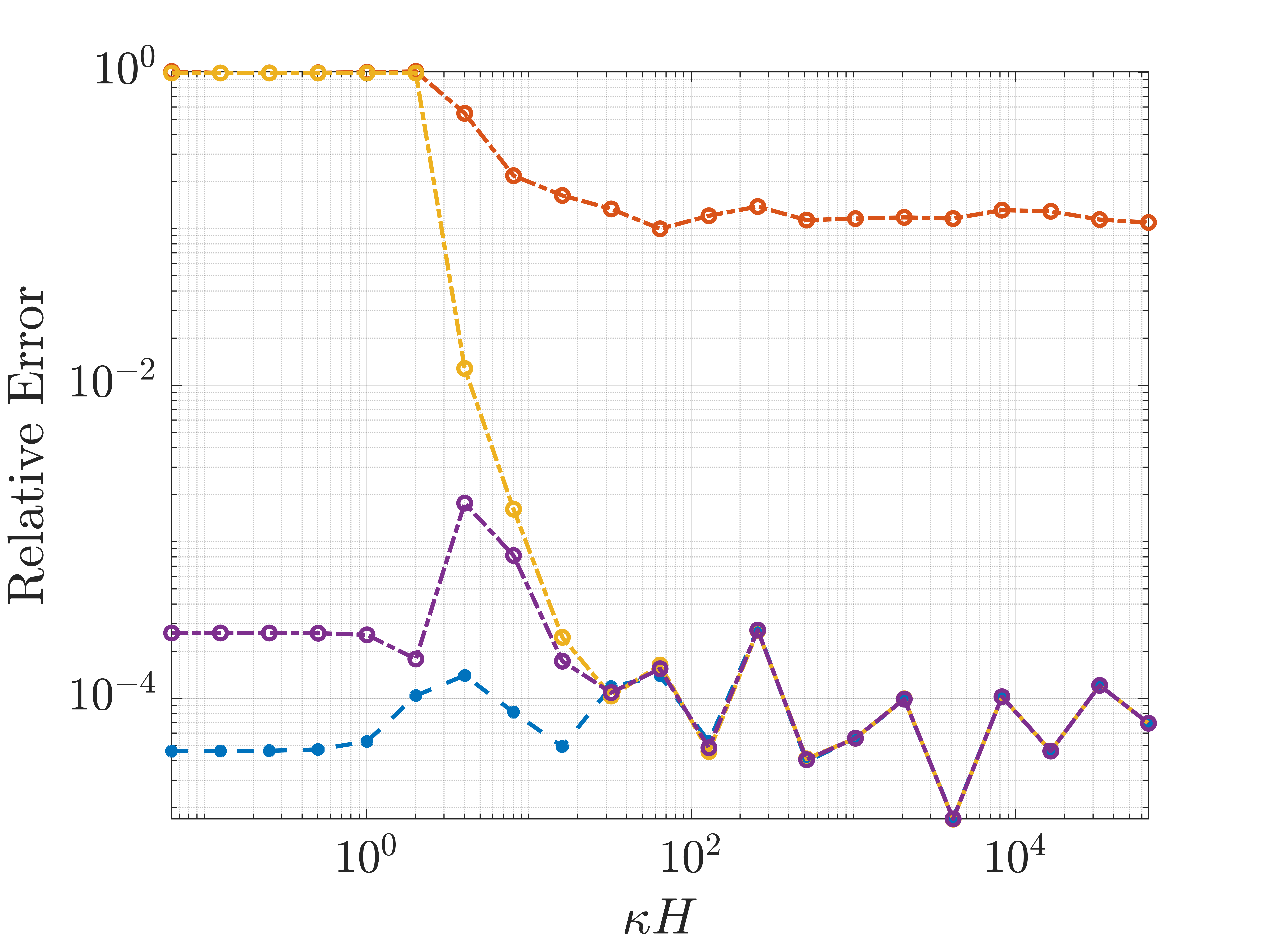
The properties of the proposed interpolation strategy, as implied by Theorem 2 (in presence of Theorem 1), are illustrated by the blue dash-dot error curves presented on the right-hand plot in Figure 4. For reference, this figure also includes error curves corresponding to various related interpolation strategies, as described below. In this demonstration the field generated by one thousand sources randomly placed within a source box $B(x_{S},H)$ of acoustic size $\kappa H$ is interpolated to one thousand points randomly placed within a cone segment of interval lengths $\Delta_{s}$ , $\Delta_{\theta}$ , and $\Delta_{\varphi}$ proportional to $\min\{1,1/(\kappa H)\}$ —which, in accordance with Theorems 1 and 2, ensures essentially constant errors. All curves in Figure 4 report errors relative to the maximum absolute value of the exact one-thousand source field value within the relevant cone segment. The target cone segment used is symmetrically located around the $x$ axis, and it lies within the $r$ range $3H/2\leq r\leq 3H/2+\Delta_{r}$ , for the value

\Delta_{r}=\frac{9H\Delta_{s}}{2\sqrt{3}(1-\sqrt{3}\Delta_{s})}

corresponding to a given value of $\Delta_{s}$ . It is useful to note that, depending on the values of $\theta$ and $\varphi$ , the distance from the closest possible singularity position to the left endpoint of the interpolation interval could vary from a distance of $H$ to a distance of $\frac{\sqrt{3}{(\sqrt{3}-1)}}{2}H\approx 0.634H$ ; cf. Figure 2(a). In all cases the interpolations were produced by means of Chebyshev expansions of degree two and four (with numerical accuracy of orders $P_{s}=3$ and $P_{\text{ang}}=5$ ) in the radial and angular directions, respectively. The ( $\kappa H$ -dependent) radial interpolation interval sizes $\Delta_{s}$ were selected as follows: starting with the value $\Delta_{s}=\sqrt{3}/3$ for $\kappa H=10^{-1}$ , $\Delta_{s}$ was varied proportionally to $1/(\kappa H)$ (resp. $\min\{1,1/(\kappa H)\}$ ) in the left-hand (resp. right-hand) plot as $\kappa H$ increases. (Note that the value $\Delta_{s}=\sqrt{3}/3$ , which corresponds to the infinite-length interval going from $r=3H/2$ to $r=\infty$ , is the maximum possible value of $\Delta_{s}$ along an interval on the $x$ axis whose distance to the source box is not smaller than one box-size $H$ . In particular, the errors presented for $\kappa H=10^{-1}$ correspond to interpolation, using a finite number of intervals, along the entire rightward $x$ semi-axis starting at $x=3H/2$ .) The corresponding angular interpolation lengths $\Delta_{\theta}=\Delta_{\varphi}$ were set to $\pi/4$ for the initial $\kappa H=10^{-1}$ value, and they were then varied like the radial interval proportionally to $1/(\kappa H)$ (resp. $\min\{1,1/(\kappa H)\}$ ) in the left-hand (resp. right-hand) plot.

As indicated above, the figure shows various interpolation results, including results for interpolation in the variable $r$ without factorization (thus interpolating the Green function (2) directly), with exponential factorization (factoring only $\exp{(\iota\kappa|x|)}$ and interpolating $\exp{(\imath\kappa(|x-x^{\prime}|-|x|)}/r$ ), with exponential and denominator factorization (called full factorization, factoring the centered factor interpolating the analytic factor as in (8)), and, finally, for the interpolation in the $s$ variable also under full factorization. It can be seen that the exponential factorization is beneficial for the interpolation strategy in the high frequency regime ( $\kappa H$ large) while the factorization of the denominator and the use of the $s$ change of variables is beneficial for the interpolation in the low frequency regime ( $\kappa H$ small). Importantly, the right-hand plot in Figure 4 confirms that, as predicted by theory, constant interval sizes in all three variables $(s,\theta,\varphi)$ suffice to ensure a constant error in the low frequency regime. Thus, the overall strategy leads to constant errors for $0\leq\kappa H<\infty$ . Figure 4 also emphasizes the significance of the factorization of the denominator, i.e. the removal of the singularity, without which interpolation with significant accuracy would be only achievable using a prohibitively large number of interpolation points. And, it also shows that the change of variables from the $r$ variable to the $s$ variable leads to a selection of interpolation points leading to improved accuracies for small values of $\kappa H$ .

Theorem 2 also holds for the special $\kappa=0$ case of the Green function for the Laplace equation. In view of its independent importance, the result is presented, in Corollary 2, explicitly for the Laplace case, without reference to the Helmholtz kernel.

Corollary 2.

Let $G^{\Delta}(x,x^{\prime})=1/|x-x^{\prime}|$ denote the Green function of the three dimensional Laplace equation and let $g_{S}^{\Delta}(x,x^{\prime})=|x|/|x-x^{\prime}|$ be denote the analytic kernel (cf. equations (5) and (8) with $\kappa=0$ ). Additionally, let $H>0$ and $\eta\in(0,1)$ be given. Then, under the change of variables $x={\mathbf{x}}(s,\theta,\varphi)$ in (11), for all $(x,x^{\prime})\in A_{\eta}^{H}$ , for all $n\in\mathbb{N}_{0}$ , and for $\xi=s$ , $\xi=\theta$ and $\xi=\varphi$ , we have

\left|\frac{\partial^{n}g^{\Delta}_{S}}{\partial\xi^{n}}\right|\leq M(\eta,n),

(26)

where $M(\eta,n)$ is a certain real constant that depends on $\eta$ and $n$ but which is independent of $H$ .

Corollary 2 shows that an even simpler and more efficient strategy can be used for the selection of the cone segment sizes in the Laplace case. Indeed, in view of Theorem 1, the corollary tells us that (as illustrated in Table 7) a constant number of cone segments per box, independent of the box size $H$ , suffices to maintain a fixed accuracy as the box size $H$ grows (as is also the case for the Helmholtz equation for small values of $\kappa$ ). As discussed in Section 4, this reduction in complexity leads to significant additional efficiency for the Laplace case.

Noting that Theorem 2 implies, in particular, that the function $g_{S}$ and all its partial derivatives with respect to the variable $s$ are bounded as $s\to 0$ , below in this section we compare the interpolation properties in the $s$ and $r$ variables, but this time in the case in which the source box is fixed and $s\to 0$ ( $r\to\infty$ ). To do this we rely in part on an upper bound on the derivatives of $g_{S}$ with respect to the variable $r$ , which is presented in Corollary 3.

Corollary 3.

Let $H>0$ and $\eta\in(0,1)$ be given. Then, under the change of variables $x={\mathbf{x}}(s,\theta,\varphi)$ in (11) and for all $(x,x^{\prime})\in A_{\eta}^{H}$ , for all $n\in\mathbb{N}_{0}$ we have

\left|\frac{\partial^{n}g_{S}}{\partial r^{n}}\right|\leq C_{r}(n,\kappa,H)\frac{1}{r^{n}}\sum\limits_{m\in I}\left(\frac{h}{r}\right)^{m},

where $I$ denotes a subset of $\{1,\ldots,n\}$ including $1$ .

Proof.

Follows directly using Theorem 2 and applying Faà di Bruno’s formula to the composition $g_{S}(s(r),\theta,\varphi)$ . ∎

Theorem 1, Theorem 2 and Corollary 3 show that, for any fixed value $\kappa H$ of the acoustic source box size, the error arising from interpolation using $n$ interpolation points in the $s$ variable (resp. the $r$ variable) behaves like $(\Delta_{s})^{n}$ (resp. $(\Delta_{r})^{n}/r^{n+1}$ ). Additionally, as is easily checked, the increments $\Delta_{s}$ and $\Delta_{r}$ are related by the identity

\Delta_{r}=\frac{r_{0}^{2}\Delta_{s}}{h-r_{0}\Delta_{s}},

(27)

where $h$ and $r_{0}$ denote the source box radius (12) and the left endpoint of a given interpolation interval $r_{0}\leq r\leq r_{0}+\Delta_{r}$ , respectively. These results and estimates lead to several simple but important conclusions. On one hand, for a given box size $\kappa H$ , a partition of the $s$ -interpolation interval $[0,\eta]$ on the basis of a finite number of equi-sized intervals of fixed size $\Delta_{s}$ (on each one of which $s$ -interpolation is to be performed) provide a natural and essentially optimal methodology for interpolation of the uniformly analytic function $g_{S}$ up to the order of accuracy desired. Secondly, such covering of the $s$ interpolation domain $[0,\eta]$ by a finite number of intervals of size $\Delta_{s}$ is mapped, via equation (11), to a covering of a complete semi-axis in the $r$ variable and, thus, one of the resulting $r$ intervals must be infinitely large—leading to large interpolation errors in the $r$ variable. Finally, values of $\Delta_{r}$ leading to constant interpolation error in the $r$ variable necessarily requires use of infinitely many interpolation intervals and is therefore significantly less efficient than the proposed $s$ interpolation approach.

Figure 5 displays interpolation errors for both the $s$ - and $r$ -interpolation strategies, for increasing values of the left endpoint $r_{0}$ and a constant source box one wavelength in side. The interval $\Delta_{s}$ is kept constant and $\Delta_{r}$ is taken per equation (27). The rightmost points in Figure 5 are close to the singular point $r_{0}=h/\Delta_{s}$ of the right-hand side in (27). The advantages of the $s$ -variable interpolation procedure are clearly demonstrated by this figure.

3.3 Algorithm

The IFGF factorization and associated box and cone interpolation strategies and structures mentioned in the previous sections underlie the full IFGF method—whose details are presented in what follows. Section 3.3.1 introduces the box and cone structures themselves, together with the associated multi-level field evaluation strategy. The notation and definitions are then incorporated in a narrative description of the full IFGF algorithm presented in Section 3.3.2. A pseudo-code for the algorithm, together with a study of the algorithmic complexity of the proposed scheme, finally, are presented in Section 3.3.3.

3.3.1 Definitions and notation

The IFGF algorithm accelerates the evaluation of the discrete operator (1) on the basis of a certain hierarchy $\mathcal{B}$ of boxes (each one of which provides a partitions of the set $\Gamma_{N}$ of discretization points). The box hierarchy, which contains, say, $D$ levels, gives rise to an intimately related hierarchy $\mathcal{C}$ of interpolation cone segments. At each level $d$ ( $1\leq d\leq D$ ), the latter $D$ -level hierarchy is embodied in a cone domain partition (cf. (17)) in $(s,\theta,\varphi)$ space—each partition amounting to a set of spherical interpolation cone segments spanning all regions of space outside certain circumscribing spheres. The details are as follows.

The level $d$ ( $1\leq d\leq D$ ) surface partitioning is produced on the basis of a total of $\left(2^{d-1}\right)^{3}$ Cartesian boxes (see Figure 7). The boxes are labeled, at each level $d$ , by means of certain level-dependent multi-indices. The hierarchy is initialized by a single box at level $d=1$ ,

B_{\mathbbm{1}}^{1}\coloneqq B(x_{\mathbbm{1}}^{1},H_{1})\quad(\text{cf.}\eqref{eq:defbox}),

(28)

containing $\Gamma_{N}$ ( $B_{\mathbbm{1}}^{1}\supset\Gamma_{N}$ ), where $H_{1}>0$ and $x_{\mathbbm{1}}^{1}\in\mathbb{R}^{3}$ denote the side and center of the box, respectively, and where, for the sake of consistency in the notation, the multi-index $\mathbbm{1}\coloneqq(1,1,1)^{T}$ is used to label the single box that exists at level $d=1$ . The box $B^{1}_{\mathbbm{1}}$ is then partitioned into eight level $d=2$ equi-sized and disjoint child boxes $B^{2}_{\mathbf{k}}$ of side $H_{2}=H_{1}/2$ ( $\mathbf{k}\in\{1,2\}^{3}$ ), which are then further partitioned into eight equi-sized disjoint child boxes $B^{3}_{\mathbf{k}}$ of side $H_{3}=H_{2}/2$ ( $\mathbf{k}\in\{1,2,3,4\}^{3}=\{1,\ldots,2^{2}\}^{3}$ ), etc. The eight-child box partitioning procedure is continued iteratively for all $1\leq d\leq D$ , at each stage halving the box along each one of the three coordinate directions $(x,y,z)$ , and thus obtaining, at level $d$ , a total of $2^{d-1}$ boxes along each coordinate axes. The partitioning procedure continues until level $d=D\in\mathbb{N}$ is reached—where $D$ is chosen in such a way that the associated box-size $H_{D}$ is sufficiently small. An illustrative two-dimensional analog of the setup for the first three levels and associated notation is presented in Figure 7(a).

As indicated above, the box-hierarchy $\mathcal{B}$ is accompanied by a cone segment hierarchy $\mathcal{C}$ . The hierarchy $\mathcal{C}$ is iteratively defined starting at level $d=D$ (which corresponds to the smallest-size boxes in the hierarchy $\mathcal{B}$ ) and moving backwards towards level $d=1$ . At each level $d$ , the cone segment hierarchy consists of a set of cone domains $E_{\gamma}^{d}$ which, together with certain related concepts, are defined following upon the discussion concerning equation (15). Thus, using $n_{s,d}$ , $n_{C,d}$ and $2n_{C,d}$ level- $d$ interpolation intervals in the $s$ , $\theta$ and $\varphi$ variables, respectively, the level- $d$ cone domains

E_{\gamma}^{d}=E_{\gamma_{1}}^{s;d}\times E_{\gamma_{2}}^{\theta;d}\times E_{\gamma_{3}}^{\varphi;d}\subset[0,\sqrt{3}/3]\times[0,\pi]\times[0,2\pi),

and its Cartesian components $E_{\gamma_{1}}^{s;d}$ , $E_{\gamma_{2}}^{\theta;d}$ and $E_{\gamma_{3}}^{\varphi;d}$ (of sizes $\Delta_{s,d}$ , $\Delta_{\theta,d}$ , and $\Delta_{\varphi,d}$ , respectively) are defined following the definition of $E_{\gamma}$ in (17) and its Cartesian components, respectively, for $n_{s}=n_{s,d}$ and $n_{C}=n_{C,d}$ , and for $\gamma=(\gamma_{1},\gamma_{2},\gamma_{3})\in K_{C}^{d}\coloneqq\{1,\ldots,n_{s,d}\}\times\{1,\ldots,n_{C,d}\}\times\{1,\ldots,2n_{C,d}\}$ . Since the parametrization $\mathbf{x}$ in (11) depends on the box size $H=H_{d}$ , and thus, on the level $d$ , the following notation for the $d$ -level parametrization is used

{\mathbf{x}}^{d}(s,\theta,\varphi)={\mathbf{x}}(\frac{\sqrt{3}H_{d}}{2r},\theta,\varphi),

(29)

which coincides with the expression (11) with $H=H_{d}$ . Using this parametrization, the level- $d$ origin-centered cone segments are then defined by

C_{\gamma}^{d}=\{\mathbf{x}^{d}(s,\theta,\varphi)\,:\,(s,\theta,\varphi)\in E_{\gamma}^{d}\}\quad\text{for all }\gamma\in K_{C}^{d},

(30)

with the resulting cone hierarchy

\mathcal{C}\coloneqq\{C_{\gamma}^{d}:1\leq d\leq D,\,\gamma\in K_{C}^{d}\}.

The interpolation segments $C_{\mathbf{k};\gamma}^{d}$ actually used for interpolation of fields resulting from sources contained within an individual level- $d$ box centered at the point $x_{\mathbf{k}}^{d}$ , are given by

C_{\mathbf{k};\gamma}^{d}\coloneqq C_{\gamma}^{d}+x_{\mathbf{k}}^{d}\quad\text{for all }\gamma\in K_{C}^{d}\text{ and }\mathbf{k}\in K^{d}.

(31)

An illustration of a two dimensional example of the cone segments and their naming scheme can be found in Figure 7(c).

Unlike the box partitioning process, which starts from a single box and proceeds from one level to the next by subdividing each parent box into $2\times 2\times 2=8$ child boxes (with refinement factors equal to two in each one of the Cartesian coordinate directions, resulting in a number $8^{d-1}$ boxes at level $d$ ), the cone segment partitioning approach proceeds iteratively downward, starting from the two $d=(D+1)$ initial cone domains

E_{(1,1,1)}^{D+1}=[0,\sqrt{3}/3]\times[0,\pi]\times[0,\pi)\quad\mbox{and}\quad E_{(1,1,2)}^{D+1}=[0,\sqrt{3}/3]\times[0,\pi]\times[\pi,2\pi).

(The initial cone domains are only introduced as the initiators of the partitioning process; actual interpolations are only performed from cone domains $E_{\gamma}^{d}$ with $D\geq d\geq 1$ .) Thus, starting at level $d=D$ and moving inductively downward to $d=1$ , the cone domains at level $d$ are obtained, from those at level $(d+1)$ , by refining each level- $(d+1)$ cone domain by level-dependent refinement factors $a_{d}$ , i.e. the number of cone segments in radial and angular directions from one level to the next is taken as $n_{s,d-1}=n_{s,d}/a_{d}$ and $n_{C,d-1}=n_{C,d}/a_{d}$ . As discussed in what follows, the refinement factors are taken to satisfy $a_{d}=1$ or $a_{d}=2$ for $D\geq d\geq 2$ , but the initial refinement value $a_{D+1}$ is an arbitrary positive integer value.

The selection of the refinement factors $a_{d}$ for $(D+1)\geq d\geq 2$ proceeds as follows. The initial refinement factor $a_{D+1}$ is chosen, via simple interpolation tests, so as to ensure that the resulting level- $D$ values $\Delta_{s,D}$ , $\Delta_{\theta,D}$ and $\Delta_{\varphi,D}$ lead to interpolation errors below the prescribed error tolerance (cf. Theorem 1). The selection of refinement factors $a_{d}$ for $d=D,D-1,\dots,2$ , in turn, also relies on Theorem 1 but, in this case, in conjunction with Theorem 2—as discussed in what follows in the case $\kappa H_{d}>1$ and, subsequently, for $\kappa H_{d}\leq 1$ . In the case $\kappa H_{d}>1$ , Theorem 2 bounds the $n$ -th derivatives of $g_{S}$ by a multiple of $(\kappa H_{d})^{n}$ . It follows that, in this case, each increase in derivative values that arise as the box size is, say, doubled, can be offset, per Theorem 1, by a corresponding decrease of the segment lengths $\Delta_{s,d}$ , $\Delta_{\theta,d}$ and $\Delta_{\varphi,d}$ by a factor of one-half. Under this scenario, therefore, as the box-size $\kappa H_{d}$ is increased by a factor of two, the corresponding parent cone segment is partitioned into eight child cone segments (using $a_{d}=2$ )—in such a way that the overall error bounds obtained via a combination of Theorems 1 and 2 remain unchanged for all levels $d$ , $1\leq d\leq D$ . Theorem 2 also tells us that, in the complementary case $\kappa H_{d}\leq 1$ (and, assuming that, additionally, $2\kappa H_{d}\leq 1$ ), for each $n$ , the $n$ -th order derivatives remain uniformly bounded as the acoustical box-size $\kappa H_{d}$ varies. In this case it follows from Theorem 1 that, as the box size is doubled and the level $d$ is decreased by one, the error level is maintained (at least as long as the $(d-1)$ -level box size $\kappa H_{d-1}=2\kappa H_{d}$ remains smaller than one), without any modification of the domain lengths $\Delta_{s,d}$ , $\Delta_{\theta,d}$ and $\Delta_{\varphi,d}$ . In such cases we set $a_{d}=1$ , so that the cone domains remain unchanged as the level transitions from $d$ to $(d-1)$ , while, as before, the error level is maintained. The special case in which $\kappa H_{d}<1$ but $2\kappa H_{d}>1$ is handled by assigning the refinement factors $a_{d}=2$ as in the $\kappa H_{d}>1$ case. Once all necessary cone domains $E_{\gamma}^{d}$ ( $D\geq d\geq 1$ ) have been determined, the cone segments $C_{\mathbf{k};\gamma}^{d}$ actually used for interpolation around a given box $B^{d}_{\mathbf{k}}\in\mathcal{B}$ are obtained via (30)-(31). A two-dimensional illustration of the multi-level cone segment structure is presented in Figure 6.

In order to take advantage of these ideas, the IFGF algorithm presented in subsequent sections relies on a set of concepts and notations—including the box and cone segment structures $\mathcal{B}$ and $\mathcal{C}$ —that are introduced in what follows. Using the notation (3), the multi-index set $K^{d}\coloneqq\{1,\ldots,2^{d-1}\}^{3}$ (which enumerates the boxes at level $d$ , $d=1,\ldots,D$ ) the initial box $B_{\mathbbm{1}}^{1}$ (equation (28)), and the iteratively defined level- $d$ box sizes and centers

H_{d}\coloneqq\frac{H_{1}}{2^{d-1}},\quad x_{\mathbf{k}}^{d}\coloneqq x_{\mathbbm{1}}^{1}-\frac{H_{1}}{2}\mathbbm{1}+\frac{H_{d}}{2}(2\mathbf{k}-\mathbbm{1})\quad(\mathbf{k}\in K^{d}),

(32)

the level- $d$ boxes and the octree $\mathcal{B}$ they bring about are given by

\displaystyle B_{\mathbf{k}}^{d}\coloneqq B(x_{\mathbf{k}}^{d},H_{d})\quad(\mathbf{k}\in K^{d}),\quad\mathcal{B}\coloneqq\{B_{\mathbf{k}}^{d}\,:\,d=1,\ldots,D,\quad\mathbf{k}\in K^{d}\};

note that, per equation (3), the boxes within the given level $d$ are mutually disjoint. The field generated, as in (6), by sources located at points within the box $B_{\mathbf{k}}^{d}$ will be denoted by

I_{\mathbf{k}}^{d}(x)\coloneqq\sum\limits_{x^{\prime}\in B_{\mathbf{k}}^{d}\cap\Gamma_{N}}a(x^{\prime})G(x,x^{\prime})=G(x,x_{\mathbf{k}}^{d})F_{\mathbf{k}}^{d}(x),\qquad F_{\mathbf{k}}^{d}(x)\coloneqq\sum\limits_{x^{\prime}\in B_{\mathbf{k}}^{d}\cap\Gamma_{N}}a(x^{\prime})g_{\mathbf{k}}^{d}(x,x^{\prime}),

(33)

where $a(x^{\prime})$ denotes the coefficient in sum (4) associated with the point $x^{\prime}$ and $g_{\mathbf{k}}^{d}=g_{S}$ the analytic factor as in (5) centered at $x_{\mathbf{k}}^{d}$ . The octree structure $\mathcal{B}$ coincides with the one used in Fast Multipole Methods (FMMs) [14, 21, 9, 12].

Typically only a small fraction of the the boxes on a given level $d$ intersect the discrete surface $\Gamma_{N}$ ; the set of all such level- $d$ relevant boxes is denoted by

\mathcal{R}_{B}^{d}\coloneqq\{B_{\mathbf{k}}^{d}\in\mathcal{B}\,:\,\mathbf{k}\in K^{d},B_{\mathbf{k}}^{d}\cap\Gamma_{N}\neq\emptyset\}.

Clearly, for each $d=1,\ldots,D$ there is a total of $N_{B}^{d}\coloneqq 2^{d-1}$ level- $d$ boxes in each coordinate direction, for a total of $(N_{B}^{d})^{3}$ level- $d$ boxes, out of which only $\mathcal{O}\left((N_{B}^{d})^{2}\right)$ are relevant boxes as $d\to\infty$ —a fact that plays an important role in the evaluation of the computational cost of the IFGF method. The set $\mathcal{N}B_{\mathbf{k}}^{d}\subset\mathcal{R}^{d}_{B}$ of boxes neighboring a given box $B_{\mathbf{k}}^{d}$ is defined as the set of all relevant level- $d$ boxes $B_{\mathbf{a}}^{d}$ such that $\mathbf{a}$ differs from $\mathbf{k}$ , in absolute value, by an integer not larger than one, in each one of the three coordinate directions: $\left\lVert\mathbf{a}-\mathbf{k}\right\rVert_{\infty}\leq 1$ . The neighborhood $\mathcal{U}B_{\mathbf{k}}^{d}\subset\mathbb{R}^{3}$ of $B_{\mathbf{k}}^{d}$ is defined by

\mathcal{U}B_{\mathbf{k}}^{d}\coloneqq\bigcup\limits_{B\in\mathcal{N}B_{\mathbf{k}}^{d}}B,\quad\mbox{where,}\quad\mathcal{N}B_{\mathbf{k}}^{d}\coloneqq\left\{B_{\mathbf{a}}^{d}\in\mathcal{R}_{B}^{d}\,:\,\left\lVert\mathbf{a}-\mathbf{k}\right\rVert_{\infty}\leq 1\right\}.

(34)

An important aspect of the proposed hierarchical algorithm concerns the application of IFGF interpolation methods to obtain field values for groups of sources within a box $B_{\mathbf{k}}^{d}$ at points farther than one box away (and thus outside the neighborhood of $B_{\mathbf{k}}^{d}$ , where either direct summation ( $d=D$ ) or interpolation from $(d+1)$ -level boxes ( $(D-1)\geq d\geq 1$ ) is applied), but that are not sufficiently far from the source box $B_{\mathbf{k}}^{d}$ to be handled by the next level, $(d-1)$ , in the interpolation hierarchy, and which must therefore be handled as part of the $d$ -level interpolation process. The associated cousin box concept is defined in terms of the hierarchical parent-child relationship in the octree $\mathcal{B}$ , wherein the parent box $\mathcal{P}B_{\textbf{k}}^{d}\in\mathcal{R}^{d-1}_{B}$ and the set $\mathcal{Q}B_{\mathbf{k}}^{d}\subset\mathcal{R}_{B}^{d+1}$ of child boxes of the box $B_{\textbf{k}}^{d}$ are defined by

	$\displaystyle\mathcal{P}B_{\textbf{k}}^{d}$	$\displaystyle\coloneqq B^{d-1}_{\mathbf{a}}\quad(\mathbf{a}\in K^{d-1})\quad\text{provided}\quad B_{\mathbf{k}}^{d}\subset B^{d-1}_{\textbf{a}},\quad\mbox{and}$
	$\displaystyle\mathcal{Q}B_{\mathbf{k}}^{d}$	$\displaystyle\coloneqq\left\{B_{\mathbf{a}}^{d+1}\in\mathcal{R}_{B}^{d+1}\,:\,\mathcal{P}B_{\mathbf{a}}^{d+1}=B_{\mathbf{k}}^{d}\text{ }\right\}.$

This leads to the notion of cousin boxes, namely, non-neighboring $(d+1)$ -level boxes which are nevertheless children of neighboring $d$ -level boxes. The cousin boxes $\mathcal{M}B_{\mathbf{k}}^{d}$ and associated cousin point sets $\mathcal{V}B_{\mathbf{k}}^{d}$ are given by

\mathcal{M}B_{\mathbf{k}}^{d}\coloneqq\left(\mathcal{R}_{B}^{d}\setminus\mathcal{N}B_{\mathbf{k}}^{d}\right)\cap\mathcal{Q}\mathcal{N}\mathcal{P}B_{\mathbf{k}}^{d}\quad\text{and}\quad\mathcal{V}B_{\mathbf{k}}^{d}\coloneqq\bigcup\limits_{B\in\mathcal{M}B_{\mathbf{k}}^{d}}B.

(35)

The concept of cousin boxes is illustrated in Figure 7(b) for a two-dimensional example, wherein the cousins of the box $B_{(2,1)}^{3}$ are shown in gray. Note that, by definition, cousin boxes of side $H$ are at a distance that is, say, no larger than $3H$ from each other. This implies that the number of cousin boxes of each box is bounded by a constant ( $6^{3}-3^{3}=189$ ) independent of the level $d$ and the number $N$ of surface discretization points.

A related set of concepts concerns the hierarchy of cone domains and cone segments. As in the box hierarchy, only a small fraction of the cone segments are relevant within the algorithm, which leads to the following definitions of cone segments $\mathcal{R}_{C}B_{\mathbf{k}}^{d}$ relevant for a box $B_{\mathbf{k}}^{d}$ , as well as the set $\mathcal{R}_{C}^{d}$ of all relevant cone segments at level $d$ . A level- $d$ cone segment $C_{\mathbf{k};\mathbf{\gamma}}^{d}$ is recursively defined to be relevant to a box $B_{\mathbf{k}}^{d}$ if either, (i) It includes a surface discretization point on a cousin of $B_{\mathbf{k}}^{d}$ , or if, (ii) It includes a point of a relevant cone segment associated with the parent box $\mathcal{P}B_{\textbf{k}}^{d}$ . In other words,

	$\displaystyle\mathcal{R}_{C}B_{\mathbf{k}}^{d}$	$\displaystyle\coloneqq\left\{C_{\mathbf{k};\mathbf{\gamma}}^{d}\,:\,\gamma\in K_{C}^{d}\,,\,C_{\mathbf{k};\mathbf{\gamma}}^{d}\cap\Gamma_{N}\cap\mathcal{V}B_{\mathbf{k}}^{d}\neq\emptyset\text{ or }C_{\mathbf{k};\mathbf{\gamma}}^{d}\cap\left(\bigcup\limits_{C\in\mathcal{R}_{C}\mathcal{P}B_{\mathbf{k}}^{d}}C\right)\neq\emptyset\right\}\quad\text{and}$
	$\displaystyle\mathcal{R}_{C}^{d}$	$\displaystyle\coloneqq\{C_{\mathbf{k};\mathbf{\gamma}}^{d}\in\mathcal{R}_{C}B_{\mathbf{k}}^{d}\,:\,\gamma\in K_{C}^{d}\,,\mathbf{k}\in K^{d}\,\mbox{and}\,B_{\mathbf{k}}^{d}\in\mathcal{R}_{B}^{d}\}.$		(36)

Clearly, whether a given cone segment is relevant to a given box on a given level $d$ depends on the relevant cone segments on the parent level $d-1$ , so that determination of all relevant cone segments can be achieved by means of a single sweep through the data structure, from $d=1$ to $d=D$ .

It is important to note that, owing to the placement of the discretization points on a two-dimensional surface $\Gamma$ in three-dimensional space, the number of relevant boxes is reduced by a factor of $1/4$ as the level is advanced from level $(d+1)$ to level $d$ (at least, asymptotically as $d\to\infty$ ). Similarly, under the cone segment refinement strategy proposed in view of Theorem 2, the overall number of relevant cone segments per box is increased by a factor of four as the box size is doubled, so that the total number of relevant cone segments remains essentially constant as $D$ grows: $|\mathcal{R}_{C}^{d}|\sim|\mathcal{R}_{C}^{d+1}|$ for all $d=1,\ldots,D-1$ as $D\to\infty$ , where $|\mathcal{R}_{C}^{d}|$ denotes the total number of relevant cone segments on level $d$ .

As discussed in Section 3.2, the cone segments $C_{\mathbf{k};\mathbf{\gamma}}^{d}$ , which are part of the IFGF interpolation strategy, are used to effect piece-wise Chebyshev interpolation in the spherical coordinate system $(s,\theta,\varphi)$ . The interpolation approach, which is based on use of discrete Chebyshev expansions, relies on use of a set $\mathcal{X}C_{\mathbf{k};\mathbf{\gamma}}^{d}$ for each relevant cone segment $C_{\mathbf{k};\mathbf{\gamma}}$ containing $P=P_{s}\times(P_{\text{ang}})^{2}$ Chebyshev interpolation points for all ${\mathbf{k}}\in K^{d}$ and $\gamma\in K_{C}^{d}$ :

\mathcal{X}C_{\mathbf{k};\mathbf{\gamma}}^{d}=\{x\in C_{\mathbf{k};\mathbf{\gamma}}^{d}\,:\,x={\mathbf{x}}^{d}(s_{k},\theta_{i},\varphi_{j})+x_{\mathbf{k}}^{d}\quad 1\leq k\leq P_{s},1\leq i\leq P_{\text{ang}},1\leq j\leq P_{\text{ang}}\},

(37)

where $s_{k}$ , $\theta_{i}$ and $\varphi_{j}$ denote Chebyshev nodes in the intervals $E_{\gamma_{1}}^{s;d}$ , $E_{\gamma_{2},\gamma_{3}}^{\theta;d}$ and $E_{\gamma_{3}}^{\varphi;d}$ , respectively, and where $x_{\mathbf{k}}^{d}$ , which is defined in (32), denotes the center of the box $B_{\mathbf{k}}^{d}$ . A two-dimensional illustration of $3\times 3$ Chebyshev interpolation points within a single cone segment can be found in Figure 7(d).

3.3.2 Narrative Description of the Algorithm

The IFGF algorithm consists of two main components, namely, precomputation and operator evaluation. The precomputation stage, which is performed only once prior to a series of operator evaluations (that may be required e.g. as part of an iterative linear-algebra solver for a discrete operator equation), initializes the box and cone structures and, in particular, it flags the relevant boxes and cone segments. The relevant boxes at each level $d$ ( $1\leq d\leq D$ ) are determined, at a cost of $\mathcal{O}(N)$ operations, by evaluation of the integer parts of the quotients of the coordinates of each point $x\in\Gamma_{N}$ by the level- $d$ box-size $H_{d}$ —resulting in an overall cost of $\mathcal{O}(N\log N)$ operations for the determination of the relevant boxes at all $D\sim\log N$ levels. Turning to determination of relevant cone segments, we first note that, since there are no cousin boxes for any box in either level $d=1$ (there is only one box in this level) or level $d=2$ (all boxes are neighbours in this level), by definition (36), there are also no relevant cone segments in levels $d=1$ and $d=2$ . To determine the relevant cone segments at level $d=3$ , in turn, the algorithm loops over all relevant boxes $B_{\mathbf{k}}^{3}\in\mathcal{R}_{B}^{3}$ , and then over all cousin target points $x\in\Gamma_{N}\cap\mathcal{V}B_{\mathbf{k}}^{3}$ of $B_{\mathbf{k}}^{3}$ , and it labels as a relevant cone segment the unique cone segment which contains $x$ . (Noting that, per definition (18), the cone segments associated with a given relevant box are mutually disjoint, the determination of the cone segment which contains the cousin point $x$ is accomplished at $\mathcal{O}(1)$ cost by means of simple arithmetic operations in spherical coordinates.) For the consecutive levels $d=4,\ldots,D$ , the same procedure as for level $d=3$ is used to determine the relevant cone segments arising from cousin points. In contrast to level $d=3$ , however, for levels $d=4,\ldots,D$ the relevant cone segments associated with the parent box $\mathcal{P}B_{\mathbf{k}}^{d}\in\mathcal{R}_{B}^{d-1}$ of a relevant box $B_{\mathbf{k}}^{d}\in\mathcal{R}_{B}^{d}$ also play a role in the determination of the relevant cone segments of the box $B_{\mathbf{k}}^{d}$ . More precisely, for $d\geq 4$ the algorithm additionally loops over all relevant cone segments $C\in\mathcal{R}_{C}\mathcal{P}B_{\mathbf{k}}^{d}$ centered at the parent box and all associated interpolation points $x\in\mathcal{X}C$ and, as with the cousin points, flags as relevant the unique cone segment $C_{\mathbf{k}}^{d}$ associated with the box $B_{\mathbf{k}}^{d}$ that includes the interpolation point $x$ .

Once the box and cone segment structures $\mathcal{B}$ and $\mathcal{C}$ have been initialized, and the corresponding sets of relevant boxes and cone segments have been determined, the IFGF algorithm proceeds to the operator evaluation stage. The algorithm thus starts at the initial level $D$ by evaluating directly the expression (33) with $d=D$ for the analytic factor $F_{\mathbf{k}}^{D}(x)$ (which contains contributions from all point sources contained in $B_{\mathbf{k}}^{D}$ ) for all level- $D$ relevant boxes $B_{\mathbf{k}}^{D}\in\mathcal{R}_{B}^{D}$ at all the surface discretization points $x\in\mathcal{U}B_{\mathbf{k}}^{D}\cap\Gamma_{N}$ neighboring $B_{\mathbf{k}}^{D}$ , as well as all points $x$ in the set $\mathcal{X}C_{\mathbf{k};\mathbf{\gamma}}^{D}$ (equation (37)) of all spherical-coordinate interpolation points associated with all relevant cone segments $C_{\mathbf{k};\mathbf{\gamma}}^{D}$ emanating from $B_{\mathbf{k}}^{D}$ . All the associated level- $D$ spherical-coordinate interpolation polynomials are then obtained through a direct computation of the coefficients (20), and the stage $D$ of the algorithm is completed by using some of those interpolants to evaluate, for all level- $D$ relevant boxes $B_{\mathbf{k}}^{D}$ , the analytic factor $F_{\mathbf{k}}^{D}(x)$ through evaluation of the sum (19), and, via multiplication by the centered factor, the field $I_{\mathbf{k}}^{D}(x)$ at all cousin target points $x\in\Gamma_{N}\cap\mathcal{V}B_{\mathbf{k}}^{D}$ . (Interpolation polynomials corresponding to regions farther away than cousins, which are obtained as part of the process just described, are saved for use in the subsequent levels of the algorithm.) Note that, under the cousin condition $x\in\Gamma_{N}\cap\mathcal{V}B_{\mathbf{k}}^{D}$ , the variable $s$ takes values on the compact subset $[0,\eta]$ ( $\eta=\sqrt{3}/3<1$ ) of the analyticity domain $0\leq s<1$ guaranteed by Corollary 1, and, thus, the error-control estimates provided in Theorem 2 guarantee that the required accuracy tolerance is met at the cousin-point interpolation step. Additionally, each cousin target point $x\in\Gamma_{N}\cap\mathcal{V}B_{\mathbf{k}}^{D}$ lies within exactly one relevant cone segment $C_{\mathbf{k};\gamma}^{D}\in\mathcal{R}_{C}B_{\mathbf{k}}^{D}$ . It follows that the evaluation of the analytic factors (33) at a point $x$ for all source boxes $B_{\mathbf{k}}^{D}$ for which $x$ is a level- $D$ cousin is an $\mathcal{O}(1)$ operation—since each surface discretization point $x\in\Gamma_{N}$ is a cousin point for no more than $189=6^{3}-3^{3}$ boxes (according to Definition (35) and the explanation following it). Therefore, the evaluation of analytic-factor cousin-box contributions at all $N$ surface discretization points requires $\mathcal{O}(N)$ operations. This completes the level- $D$ portion of the IFGF algorithm.

At the completion of the level- $D$ stage the field $I_{\mathbf{k}}^{D}(x)$ generated by each relevant box $B_{\mathbf{k}}^{D}$ has been evaluated at all neighbor and cousin surface discretization points $x\in\Gamma_{N}\cap\left(\mathcal{U}B_{\mathbf{k}}^{D}\cup\mathcal{V}B_{\mathbf{k}}^{D}\right)$ , but field values at surface points farther away from sources, $x\in\Gamma_{N}\setminus\left(\mathcal{U}B_{\mathbf{k}}^{D}\cup\mathcal{V}B_{\mathbf{k}}^{D}\right)$ , still need to be obtained; these are produced at stages $d=D-1,\ldots,3$ . (The evaluation process is indeed completed at level $d=3$ since by construction we have $\mathcal{U}B_{\mathbf{k}}^{3}\cup\mathcal{V}B_{\mathbf{k}}^{3}\supset\Gamma_{N}$ for any $\mathbf{k}\in K^{3}$ .) For each relevant box $B_{\mathbf{k}}^{d}\in\mathcal{R}_{B}^{d}$ , the level- $d$ algorithm ( $(D-1)\geq d\geq 3$ ) proceeds by utilizing the previously calculated $(d+1)$ -level spherical-coordinate interpolants for each one of the relevant children of $B_{\mathbf{k}}^{d}$ , to evaluate the analytic factor $F_{\mathbf{k}}^{d}(x)$ generated by sources contained within $B_{\mathbf{k}}^{d}$ at all points $x$ in all the sets $\mathcal{X}C_{\mathbf{k};\gamma}^{d}$ (equation (37)) of spherical-coordinate interpolation points associated with relevant cone segments $C_{\mathbf{k};\gamma}^{d}{\color[rgb]{0,0,0}\in\mathcal{R}_{C}B_{\mathbf{k}}^{d}}$ emanating from $B_{\mathbf{k}}^{d}$ , which are then used to generate the level- $d$ Chebyshev interpolants through evaluation of the sums (20). The level- $d$ stage is then completed by using some of those interpolants to evaluate, for all level- $d$ relevant boxes $B_{\mathbf{k}}^{d}$ , the analytic factor $F_{\mathbf{k}}^{d}(x)$ and, by multiplication with the centered factor, the field $I_{\mathbf{k}}^{d}(x)$ , at all cousin target points $x\in\Gamma_{N}\cap\mathcal{V}B_{\mathbf{k}}^{d}$ . As in the level $D$ case, these level- $d$ interpolations are performed at a cost of $\mathcal{O}(N)$ operations for all surface discretization points—since, as in the level- $D$ case, each surface discretization point (i) Is a cousin target point of $\mathcal{O}(1)$ boxes, and (ii) Is contained within one cone segment per cousin box. This completes the algorithm.

As indicated in the Introduction, the IFGF method does not require a downward pass through the box tree structure—of the kind required by FMM approaches—to evaluate the field at the surface discretization points. Instead, as indicated above, in the IFGF algorithm the surface-point evaluation is performed as part of a single (upward) pass throught the tree structure, with increasing box sizes $H_{d}$ and decreasing values of $d$ , as the interpolating polynomials associated with the various relevant cone segments are evaluated at cousin surface points. Thus, the IFGF approach aggregates contributions arising from large numbers of point sources, but, unlike the FMM, it does so using large number of interpolants of a low (and fixed) degree over decreasing angular and radial spans, instead of using expansions of increasingly large order over fixed angular and radial spans.

It is important to note that, in order to achieve the desired acceleration, the algorithm evaluates analytic factors $F_{\mathbf{k}}^{d}(x)$ arising from a level- $d$ box $B_{\mathbf{k}}^{d}$ , whether at interpolation points $x$ in the subsequent level, or for cousin surface discretization points $x$ , by relying on interpolation based on (previously computed) interpolation polynomials associated with the $(d+1)$ -level relevant children boxes of $B_{\mathbf{k}}^{d}$ , instead of directly evaluating $I_{\mathbf{k}}^{d}(x)$ using equation (33). In particular, all interpolation points within relevant cone segments on level $d$ are also targets of the interpolation performed on level $(d+1)$ . Evaluation of interpolant at surface discretization points $x\in\Gamma_{N}$ , on the other hand, are restricted to cousin surface points: evaluation at all points farther away are deferred to subsequent larger-box stages of the algorithm.

Of course, the proposed interpolation strategy requires the creation, for each level- $d$ relevant box $B_{\mathbf{k}}^{d}$ , of all level- $d$ cone segments and interpolants necessary to cover both the cousin surface discretization points as well as all of the interpolation points in the relevant cone segments on level $(d-1)$ . We emphasize that the interpolation onto interpolation points requires a re-centering procedure consisting of multiplication by the level $d$ centered factors, and division by corresponding level- $(d-1)$ centered factors (cf equation (33)). We note that, in particular, this re-centering procedure (whose need arises as a result of the algorithm’s reliance on the coordinate transformation (29) but re-centered at the $d$ -level cube centers for varying values of $d$ ) causes the set of the children cone segments not to be geometrically contained within the corresponding parent cone segment (cf. Figure 6(b)). The procedure of interpolation onto interpolation points, which is, in fact, an iterated Chebyshev interpolation method, does not result in error amplification—as it follows from a simple variation of Theorem 1.

Using the notation in Section 3.3.1, the IFGF algorithm described above is summarized in its entirety in what follows.

•
Initialization of relevant boxes and relevant cone segments.
- –
  
  Determine the sets $\mathcal{R}_{B}^{d}$ and $\mathcal{R}_{C}^{d}$ for all $d=1,\ldots,D$ .
•
Direct evaluations on level $D$ .
- –
  
  For every $D$ -level box $B_{\mathbf{k}}^{D}\in\mathcal{R}_{B}^{D}$ evaluate the analytic factor $F_{\mathbf{k}}^{D}(x)$ generated by point sources within $B_{\mathbf{k}}^{D}$ at all neighboring surface discretization points $x\in\Gamma_{N}\cap\mathcal{U}B_{\mathbf{k}}^{D}$ by direct evaluation of equation (33).
- –
  
  For every $D$ -level box $B_{\mathbf{k}}^{D}\in\mathcal{R}_{B}^{D}$ evaluate the analytic factor $F_{\mathbf{k}}^{D}(x)$ at all interpolation points $x\in\mathcal{X}C_{\mathbf{k};\mathbf{\gamma}}^{D}$ for all $C_{\mathbf{k};\mathbf{\gamma}}^{D}\in\mathcal{R}_{C}B_{\mathbf{k}}^{D}$ .
•
Interpolation, for $d=D,\ldots,3$ .
- –
  
  For every every box $B_{\mathbf{k}}^{d}$ evaluate the field $I_{\mathbf{k}}^{d}(x)$ (equation (33)) at every surface discretization point $x$ within the cousin boxes of $B_{\mathbf{k}}^{d}$ , $x\in\Gamma_{N}\cap\mathcal{V}B_{\mathbf{k}}^{d}$ , by interpolation of $F_{\mathbf{k}}^{d}$ and multiplication by the centered factor $G(x,x_{\mathbf{k}}^{d})$ .
- –
  
  For every every box $B_{\mathbf{k}}^{d}$ determine the parent box $B_{\mathbf{j}}^{d-1}=\mathcal{P}B_{\mathbf{k}}^{d}$ and, by way of interpolation of the analytic factor $F_{\mathbf{k}}^{d}$ and re-centering by the smooth factor $G(x,x_{\mathbf{k}}^{d})/G(x,x_{\mathbf{j}}^{d-1})$ , obtain the values of the parent-box analytic factors $F_{\mathbf{j}}^{d-1}$ at all level- $(d-1)$ interpolation points corresponding to $B_{\mathbf{j}}^{d-1}$ —that is to say, at all points $x\in\mathcal{X}C_{\mathbf{j};\mathbf{\gamma}}^{d-1}$ for all $C_{\mathbf{j};\mathbf{\gamma}}^{d-1}\in\mathcal{R}_{C}B_{\mathbf{j}}^{d-1}$ (Note: the contributions of all the children of $B_{\mathbf{j}}^{d-1}$ need to be accumulated at this step.)

The corresponding pseudo code, Algorithm 1, is presented in the following section.

3.3.3 Pseudo-code and Complexity

1: \\Initialization.

2: for

d=1,\ldots,D

3: Determine relevant boxes

\mathcal{R}^{d}_{B}

and cone segments

\mathcal{R}_{C}^{d}

4: end for

6: \\Direct evaluations on the lowest level.

7: for

B_{\mathbf{k}}^{D}\in\mathcal{R}_{B}^{D}

8: for

x\in\mathcal{U}B^{D}_{\mathbf{k}}\cap\Gamma_{N}

\triangleright

Direct evaluations onto neighboring surface points

9: Evaluate

I_{\mathbf{k}}^{D}(x)

10: end for

11: for

C_{\mathbf{k};\mathbf{\gamma}}^{D}\in\mathcal{R}_{C}B_{\mathbf{k}}^{D}

\triangleright

Evaluate

F

on all relevant interpolation points

12: for

x\in\mathcal{X}C_{\mathbf{k};\mathbf{\gamma}}^{D}

13: Evaluate and store

F_{\mathbf{k}}^{D}(x)

14: end for

15: end for

16: end for

17:

18: \\Interpolation onto surface discretization points and parent interpolation points.

19: for

d=D,\ldots,3

20: for

B_{\mathbf{k}}^{d}\in\mathcal{R}_{B}^{d}

21: for

x\in\mathcal{V}B_{\mathbf{k}}^{d}\cap\Gamma_{N}

\triangleright

Interpolate at cousin surface points

22: Evaluate

I_{\mathbf{k}}^{d}(x)

by interpolation

23: end for

24: if

d>3

then

\triangleright

Evaluate

F

on parent interpolation points

25: Determine parent

B_{\mathbf{j}}^{d-1}=\mathcal{P}B_{\mathbf{k}}^{d}

26: for

C_{\mathbf{j};\mathbf{\gamma}}^{d-1}\in\mathcal{R}_{C}B_{\mathbf{j}}^{d-1}

27: for

x\in\mathcal{X}C_{\mathbf{j};\mathbf{\gamma}}^{d-1}

28: Evaluate and add

F_{\mathbf{k}}^{d}(x)G(x,x_{\mathbf{k}}^{d})/G(x,x_{\mathbf{j}}^{d-1})

29: end for

30: end for

31: end if

32: end for

33: end for

Algorithm 1 IFGF Method

As shown in what follows, under the assumption, natural in the surface scattering context assumed in this paper, that the wavenumber $\kappa$ does not grow faster than $\mathcal{O}(\sqrt{N})$ , the IFGF Algorithm 1 runs at an asymptotic computational cost of $\mathcal{O}(N\log N)$ operations. The complexity estimates presented in this section incorporate the fundamental assumptions inherent throughout this paper that fixed interpolation orders $P_{s}$ and $P_{\text{ang}}$ , and, thus, fixed numbers $P$ of interpolation points per cone segment, are utilized.

For a given choice of interpolation orders $P_{s}$ and $P_{\text{ang}}$ , the algorithm is completely determined once the number $D$ of levels and the numbers $n_{s,D}$ and $n_{C,D}$ of level- $D$ radial and angular interpolation intervals are selected. For a particular configuration, the parameters $D$ , $n_{s,D}$ and $n_{C,D}$ should be chosen in such a way that the overall computational cost is minimized while meeting a given accuracy requirement. An increasing number $D$ of levels reduces the cost of the direct neighbour-evaluations by performing more of them via interpolation to cousin boxes—which increases the cost of that particular part of the algorithm. The choice of $D$ , $n_{s,D}$ and $n_{C,D}$ should therefore be such that the overall cost of these two steps is minimized while meeting the prescribed accuracy—thus achieving optimal runtime for the overall IFGF method. Note that these selections imply that, for bounded values of $n_{s,D}$ and $n_{C,D}$ (e.g., we consistently use $n_{s,D}=1$ and $n_{C,D}=2$ in all of our numerical examples) it follows that $D=\mathcal{O}(\log N)$ —since, as it can be easily checked, e.g. increasing $N\to 4N$ and $D\to D+1$ maintains the aforementioned optimality of the choice of the parameter $D$ . In sum, the IFGF algorithm satisfies the following asymptotics as $\kappa\to\infty$ : $\kappa^{2}=\mathcal{O}(N)$ , $D=\mathcal{O}(\log{N})$ , $|\mathcal{R}_{C}^{d}|=\mathcal{O}(1)$ and $|\mathcal{R}_{B}^{D}|=\mathcal{O}(N)$ .

The complexity of the IFGF algorithm equals the number of arithmetic operations performed in Algorithm 1. To evaluate this complexity we first consider the cost of the level $D$ specific evaluations performed in the “for loop” starting in Line 7. This loop iterates for a total of $\mathcal{O}(N)$ times. The inner loop starting in Line 8, in turn, performs $\mathcal{O}(1)$ iterations, just like the loops in the Lines 11 and 12. In total this yields an algorithmic complexity of $\mathcal{O}(N)$ operations.

We consider next the section of the algorithm contained in the loop starting in Line 19, which iterates $\mathcal{O}(\log N)$ times (since $D\sim\log N$ ). The loop in Line 20, in turn, iterates $\mathcal{O}(N/4^{D-d})$ times, since the number of relevant boxes is asymptotically decreased by a factor of $1/4$ as the algorithm progresses from a given level $d$ to the subsequent level $d-1$ . Similarly, the loop in Line 21 performs $\mathcal{O}(4^{D-d})$ iterations—since, as the algorithm progresses from level $d$ to level $d-1$ , the side $H$ of the cousin boxes increases by a factor of two, and thus, the number of cousin discrete surface points for each relevant box increases by a factor of four. The interpolation procedure in Line 22, finally, is an $\mathcal{O}(1)$ operation since each point $x$ lies in exactly one cone segment associated with a given box $B_{\mathbf{k}}^{d}$ (cf. Definition (18) of the cone segments and the previous discussion in Section 3.3.2) and the interpolation therefore only requires the evaluation of a single fixed order Chebyshev interpolant. A similar count as for the loop in Line 21 holds for the loop in Line 26 which is also run $\mathcal{O}(4^{D-d})$ times since, going from a level $d$ to the parent level $d-1$ , the number of relevant cone segments per box increases by a factor four. The “for” loop in Line 27 is performed $\mathcal{O}(1)$ times since the number of interpolation points per cone segment is constant. Altogether, this yields the desired $\mathcal{O}(N\log N)$ algorithmic complexity.

In the particular case $\kappa=0$ the cost of the algorithm is still $\mathcal{O}(N\log N)$ operations, in view of the $\mathcal{O}(N\log N)$ cost required by the interpolation to surface points. But owing to the reduced cost of the procedure of interpolation to parent-level interpolation points, which results as a constant number of cone segments per box suffices for $\kappa H_{d}<1$ (cf. Section 3.2), the overall $\kappa=0$ IFGF algorithm is significantly faster than it is for cases in which $\kappa H_{d}>1$ for some levels $d$ . In fact, it is expected that an algorithmic complexity of $\mathcal{O}(N)$ operations should be achievable by a suitable modification of algorithm in the Laplace case $\kappa=0$ , but this topic is not explored in this paper at any length.

Finally, we consider the algorithmic complexity of the pre-computation stage, namely, the loop starting in Line 2. But according to the first paragraph in Section 3.3.2, the algorithm corresponding to Line 3 is executed at a computing cost of $\mathcal{O}(N)$ operations. It follows that the full Line 2 loop runs at $\mathcal{O}(N\log N)$ operations, since $D=\mathcal{O}(\log N)$ .

4 Numerical Results

We analyze the performance of the proposed IFGF approach by considering the computing time and memory required by the algorithm to evaluate the discrete operator (1) for various $N$ -point surface discretizations. In each case, the tests concern the accelerated evaluation of the full $N$ -point sum (1) at each one of $N$ discretization points $x_{\ell}$ , $\ell=1,\dots,N$ —which, if evaluated by direct addition would require a total of $\mathcal{O}(N^{2})$ operations. We consider various configurations, including examples for the Helmholtz ( $\kappa\neq 0$ ) and Laplace ( $\kappa=0$ ) Green functions, and for four different geometries, namely, a sphere of radius $a$ , an oblate (resp. prolate) spheroid of the form

\left\{(x,y,z)\in\mathbb{R}^{3}\,:\,\frac{x^{2}}{\alpha^{2}}+\frac{y^{2}}{\beta^{2}}+\frac{z^{2}}{\gamma^{2}}=a^{2}\right\},

(38)

with $\alpha=\beta=1$ and $\gamma=0.1$ (resp. $\alpha=\beta=0.1$ and $\gamma=1$ ), and the rough radius $\approx a$ sphere defined by

\left\{x=\tilde{\mathbf{x}}\left(a[1+0.05\sin{(40\theta)}\sin{(40\varphi)}],\hskip 2.5pt\theta,\hskip 2.5pt\varphi\right)\,:\,\tilde{\mathbf{x}}\text{ as in }\eqref{eq:defparametrizationr},\hskip 2.5pt\theta\in[0,\pi],\hskip 2.5pt\varphi\in[0,2\pi)\right\}.

(39)

The oblate spheroid and rough sphere are depicted in Figures 8(b) and 8(a), respectively.

All tests were performed on a Lenovo X1 Extreme 2018 Laptop with an Intel i7-8750H Processor and 16 GB RAM running Ubuntu 18.04 as operating system. The code is a single core implementation in C++ of Algorithm 1 compiled with the Intel C++ compiler version 19 and without noteworthy vectorization. Throughout all tests, $T_{\text{acc}}$ denotes the time required for a single application of the IFGF method and excludes the pre-computation time $T_{\text{pre}}$ (which is presented separately in each case, and which includes the time required for setup of the data structures and the determination of the relevant boxes and cone segments), but which includes all the other parts of the algorithm presented in Section 3.3, including the direct evaluation at the neighboring surface discretization points on level $D$ . Throughout this Section, solution accuracies were estimated on the basis of the relative $L_{2}$ error norm

{\color[rgb]{0,0,0}\varepsilon_{M}=\sqrt{\frac{\sum\limits_{i=1}^{M}|I(x_{\sigma(i)})-I_{\text{acc}}(x_{\sigma(i)})|^{2}}{\sum\limits_{i=1}^{M}|I(x_{\sigma(i)})|^{2}}},}

(40)

on a subset of $M=1000$ points chosen randomly (using a random permutation $\sigma$ of the set of positive integers less than equal to $N$ ) among the $N$ surface discretization points $\{x_{\ell}:\ell=1,\dots,N\}$ (cf. equation (1)). Here, for a given $x\in\Gamma_{N}$ , $I(x)$ and $I_{\text{acc}}(x)$ denote the exact and accelerated evaluation, respectively, of the discrete operator (1) at the point $x$ . To ensure that $M=1000$ gives a sufficiently accurate approximation of the error, the exact relative errors $\varepsilon_{N}$ accounting for all $N$ surface discretization points were also obtained for the first three test cases shown in Table 1; the results are $\varepsilon_{N}=3.56\times 10^{-4}$ ( $N=24576$ ), $\varepsilon_{N}=5.71\times 10^{-4}$ ( $N=98304$ ) and $\varepsilon_{N}=9.28\times 10^{-4}$ ( $N=393216$ ). (Exact relative error evaluation for larger values of $N$ is not practical on account of the prohibitive computation times required by the non-accelerated operator evaluation.) The table columns display the number PPW of surface discretization points per wavelength, the total number $N$ of surface discretization points and the wavenumber $\kappa$ . The PPW are computed on the basis of the number of surface discretization points along the equator of a sphere (even for the rough-sphere case), or the largest equator in the case of spheroids. Note that the PPW have no impact on the accuracy of the IFGF acceleration, since only the discrete operator (1) is evaluated in the present context, instead of an accurate approximation of a full continuous operator. The PPW are only considered here as they provide an indication of the discretization levels that might be used to achieve continuous operator approximations with errors consistent with those displayed in the various tables presented in this section. The memory column displays the peak memory required by the algorithm.

In all the tests where the Helmholtz Green function is used, the number of levels $D$ in the scheme is chosen in such a way that the resulting smallest boxes on level $D$ are approximately a quarter wavelength in size ( $H_{D}\approx 0.25\lambda$ ). Moreover, for the sake of simplicity, the version of the IFGF algorithm described in Section 3.3 does not incorporate an adaptive box octree (which would stop the partitioning process once a given box contains a sufficiently small number of points) but instead always partitions boxes until the prescribed level $D$ is reached. Hence, a box is a leaf in the tree if and only if it is a level- $D$ box. This can lead to large deviations in the number of surface points within boxes, in the number of relevant boxes and in the number of relevant cone segments. These deviations may result in slight departures from the predicted $\mathcal{O}(N\log N)$ costs in terms of memory requirements and computing time. The cone segments (as defined in (16)) are chosen in such a way that there are eight cone segments ( $1\times 2\times 4$ segments in the $s$ , $\theta$ and $\varphi$ variables, respectively) associated with each of the smallest boxes on level $D$ and they are refined according to Section 3.2 for the levels $d<D$ . Unless stated otherwise, each cone segment is assigned $P=P_{s}\times P_{\text{ang}}\times P_{\text{ang}}$ interpolation points with $P_{s}=3$ and $P_{\text{ang}}=5$ . We note that both, the point evaluation of Chebyshev polynomials and the computation of Chebyshev coefficients, are performed on the basis of simple evaluations of triple sums without employing any acceleration methods such as FFTs.

The first test investigates the scaling of the algorithm as the surface acoustic size is increased and the number of surface discretization points $N$ is increased proportionally to achieve a constant number of points per wavelength. The results of these tests are presented in the Tables 1, 2, and 3 for the aforementioned radius- $a$ sphere, the oblate spheroid (38) (for $\alpha=\beta=1$ , $\gamma=0.1$ ) and rough sphere (39), respectively. The acoustic sizes of the test geometries range from $4$ wavelengths to $64$ wavelengths in diameter for the normal and rough sphere cases, and up to $128$ wavelengths in large diameter for the case of the oblate spheroid.

$N$	$\mathbf{\kappa}a$	PPW	$\mathbf{\varepsilon}$	$T_{\text{pre}}$ (s)	$T_{\text{acc}}$ (s)	Memory (MB)
$24576$	$4\pi$	$22.4$	$3.57\times 10^{-4}$	$5.25\times 10^{-1}$	$1.81\times 10^{0}$	$25$
$98304$	$8\pi$		$5.77\times 10^{-4}$	$3.33\times 10^{0}$	$9.30\times 10^{0}$	$80$
$393216$	$16\pi$		$9.31\times 10^{-4}$	$1.86\times 10^{1}$	$4.55\times 10^{1}$	$315$
$1572864$	$32\pi$		$1.49\times 10^{-3}$	$9.74\times 10^{1}$	$2.21\times 10^{2}$	$1308$
$6291456$	$64\pi$		$1.99\times 10^{-3}$	$4.89\times 10^{2}$	$1.05\times 10^{3}$	$5396$

Table 1: Computing times

T_{\text{acc}}

required by the IFGF accelerator for a sphere of radius

a

, with

(P_{s},P_{\text{ang}})=(3,5)

, and for various numbers

N

of surface discretization points and wavenumbers

\kappa a

—at a fixed number of points-per-wavelength. The pre-computation times

T_{\text{pre}}

, the resulting relative accuracy

\varepsilon

and the peak memory used are also displayed.

$N$	$\mathbf{\kappa}a$	PPW	$\mathbf{\varepsilon}$	$T_{\text{pre}}$ (s)	$T_{\text{acc}}$ (s)	Memory (MB)
$24576$	$4\pi$	$22.4$	$1.18\times 10^{-4}$	$1.30\times 10^{-1}$	$1.44\times 10^{0}$	$17$
$98304$	$8\pi$		$1.82\times 10^{-4}$	$1.15\times 10^{0}$	$6.52\times 10^{0}$	$42$
$393216$	$16\pi$		$2.26\times 10^{-4}$	$5.03\times 10^{0}$	$2.87\times 10^{1}$	$158$
$1572864$	$32\pi$		$2.55\times 10^{-4}$	$2.63\times 10^{1}$	$1.31\times 10^{2}$	$605$
$6291456$	$64\pi$		$2.83\times 10^{-4}$	$1.30\times 10^{2}$	$5.72\times 10^{2}$	$2273$
$25165824$	$128\pi$		$3.61\times 10^{-4}$	$6.27\times 10^{2}$	$2.64\times 10^{3}$	$9264$

Table 2: Same as Table 1 but for an oblate spheroid of equation

x^{2}+y^{2}+(z/0.1)^{2}=a^{2}

depicted in Figure 8(b).

$N$	$\mathbf{\kappa}a$	PPW	$\mathbf{\varepsilon}$	$T_{\text{pre}}$ (s)	$T_{\text{acc}}$ (s)	Memory (MB)
$24576$	$4\pi$	$22.4$	$2.90\times 10^{-4}$	$5.90\times 10^{-1}$	$1.90\times 10^{0}$	$26$
$98304$	$8\pi$		$3.26\times 10^{-4}$	$4.12\times 10^{0}$	$1.08\times 10^{1}$	$97$
$393216$	$16\pi$		$5.08\times 10^{-4}$	$2.58\times 10^{1}$	$6.11\times 10^{1}$	$463$
$1572864$	$32\pi$		$2.66\times 10^{-4}$	$1.47\times 10^{2}$	$3.28\times 10^{2}$	$2131$
$6291456$	$64\pi$		$2.56\times 10^{-4}$	$7.77\times 10^{2}$	$1.66\times 10^{3}$	$10502$

Table 3: Same as Table 1 but for the rough sphere

r=a(1+0.05\sin{(40\theta)}\sin{(40\varphi)})

depicted in Figure 8(a).

Several key observations may be drawn from these results. On one hand we see that, in all cases the computing and memory costs of the method scale like $\mathcal{O}(N\log N)$ , thus yielding the expected improvement over the $\mathcal{O}(N^{2})$ costs required by the straightforward non-accelerated algorithm. Additionally, we note that the computational times and memory required for a given $N$ , which are essentially proportional to the number of relevant cone segments used, depend on the character of the surface considered (since the number of relevant cone segments used is heavily dependent on the surface character), and they can therefore give rise to significant memory and computing-cost variations in some cases. For the oblate spheroid case, for example, the number of relevant cone segments in upward- and downward-facing cone directions is significantly smaller than the number for the regular sphere case, whereas the rough sphere requires significantly more relevant cone segments than the regular sphere, especially in the $s$ variable, to span the thickness of the roughness region.

Table 4 demonstrates the scaling of the IFGF method for a fixed number $N$ of surface discretization points and increasing wavenumber $\kappa a$ for the sphere geometry. The memory requirements and the timings also scale like $\mathcal{O}(\kappa^{2}\log\kappa)$ since the interpolation to interpolation points used in the algorithm is independent of $N$ and scales like $\mathcal{O}(\kappa^{2}\log\kappa)$ . But the time required for the interpolation back to the surface depends on $N$ and is therefore constant in this particular test—which explains the slight reductions in overall computing times for a given value of $\kappa a$ over the ones displayed in Table 1 for the case in which $N$ is scaled proportionally to $\kappa a$ .

$N$	$\mathbf{\kappa}a$	PPW	$\mathbf{\varepsilon}$	$T_{\text{pre}}$ (s)	$T_{\text{acc}}$ (s)	Memory (MB)
$393216$	$16\pi$	$22.4$	$9.31\times 10^{-4}$	$1.86\times 10^{1}$	$4.55\times 10^{1}$	$315$
	$32\pi$	$11.2$	$1.13\times 10^{-3}$	$8.17\times 10^{1}$	$1.33\times 10^{2}$	$1032$
	$64\pi$	$5.6$	$1.29\times 10^{-3}$	$3.73\times 10^{2}$	$5.63\times 10^{2}$	$3927$

Table 4: Same as Table 1 but for a fixed number

N

of surface discretization points, demonstrating the scaling of the algorithm as

\kappa a

is increased independently of the discretization size while maintaining the accelerator’s accuracy.

Table 5 shows a similar sphere test but for a sphere of constant acoustic size and with various numbers $N$ of surface discretization points. As we found earlier, the computation times and memory requirements scale like $\mathcal{O}(N\log N)$ (the main cost of which stems from the process of interpolation back to the surface discretization points; see Line 21 in Algorithm 1). Since the cost of the IFGF method (in terms of computation time and memory requirements) is usually dominated by the cost of the interpolation to interpolation points ( Line 26 in Algorithm 1), which is only dependent on the wavenumber $\kappa a$ , the scaling in $N$ is better than $\mathcal{O}(N\log N)$ until $N$ is sufficiently large, so that the process of interpolation back to the surface discretization points requires a large enough portion of the share of the overall computing time—as observed in the fourth and fifth rows in Table 5.

$N$	$\mathbf{\kappa}a$	PPW	$\mathbf{\varepsilon}$	$T_{\text{pre}}$ (s)	$T_{\text{acc}}$ (s)	Memory (MB)
$24576$	$16\pi$	$5.6$	$2.90\times 10^{-4}$	$9.30\times 10^{0}$	$1.66\times 10^{1}$	$228$
$98304$		$11.2$	$5.54\times 10^{-4}$	$1.13\times 10^{1}$	$2.23\times 10^{1}$	$267$
$393216$		$22.4$	$9.09\times 10^{-4}$	$1.40\times 10^{1}$	$4.14\times 10^{1}$	$320$
$1572864$		$44.8$	$1.04\times 10^{-3}$	$2.34\times 10^{1}$	$1.63\times 10^{2}$	$498$

Table 5: Same as Table 1 but for a fixed acoustic size

\kappa a

, demonstrating the scaling of the algorithm as

N

is increased independently of the acoustic size.

Table 6 displays results produced by the IFGF method for the prolate spheroid (38) with $\alpha=\beta=0.1$ and $\gamma=1$ at relative error levels $\varepsilon\approx 10^{-2}$ . The test demonstrates highly competitive results in terms of memory requirements and computation time for geometries as large as 512 wavelengths in size. The method exhibits similar efficiency for the sphere and the oblate spheroid geometries at the levels of accuracy presented in Table 6.

$N$	$\mathbf{\kappa}a$	PPW	$\mathbf{\varepsilon}$	$T_{\text{pre}}$ (s)	$T_{\text{acc}}$ (s)	Memory (MB)
$393216$	$16\pi$	$22.4$	$2.43\times 10^{-3}$	$2.21\times 10^{0}$	$2.19\times 10^{1}$	$98$
$1572864$	$32\pi$		$5.75\times 10^{-3}$	$1.16\times 10^{1}$	$9.75\times 10^{1}$	$371$
$6291456$	$64\pi$		$8.29\times 10^{-3}$	$5.70\times 10^{1}$	$4.24\times 10^{2}$	$1316$
$25165824$	$128\pi$		$9.84\times 10^{-3}$	$2.72\times 10^{2}$	$1.85\times 10^{3}$	$5317$
$25165824$	$256\pi$	$11.2$	$1.23\times 10^{-2}$	$3.89\times 10^{2}$	$2.05\times 10^{3}$	$5470$
$25165824$	$512\pi$	$5.6$	$1.52\times 10^{-2}$	$1.01\times 10^{3}$	$2.57\times 10^{3}$	$10685$

Table 6: Same as Table 1 but for a prolate spheroid of equation

(x/0.1)^{2}+(y/0.1)^{2}+z^{2}=a^{2}

and a target accuracy of

\varepsilon=10^{-2}

(cf. the second paragraph in the present section with regards to the selection of PPW in each case).

In our final example, we consider an application of the IFGF method to a spherical geometry for the Laplace equation. The results are shown in Table 7. A perfect $\mathcal{O}(N\log N)$ scaling is observed. Note that the portion of the algorithm “interpolation to interpolation points” (Line 26 in Algorithm 1), which requires a significant fraction of the computing time in the Helmholtz case, runs at a negligible cost in the Laplace case—for which a constant number of cone segments can be used throughout all levels, as discussed in Section 3.2.

$N$	$\mathbf{\varepsilon}$	$T_{\text{acc}}$ (s)	Memory (MB)
$24576$	$1.51\times 10^{-5}$	$7.81\times 10^{-1}$	$25$
$98304$	$1.38\times 10^{-5}$	$3.62\times 10^{0}$	$69$
$393216$	$1.27\times 10^{-5}$	$1.69\times 10^{1}$	$246$
$1572864$	$1.34\times 10^{-5}$	$7.45\times 10^{1}$	$962$
$6291456$	$1.77\times 10^{-5}$	$3.29\times 10^{2}$	$3676$

Table 7: Same as Table 1 but for the Laplace equation (

\kappa a=0

). The pre-computation times (not shown) are negligible in this case, since the most cost-intensive part of the pre-computation algorithm, namely, the determination of the relevant cone segments, is not necessary in the present Laplace context. Per the IFGF Laplace algorithmic prescription, a fixed number of cone segments per box is used across all levels in the hierarchical data structure.

Another possible optimization which was not used for the IFGF method but for the method presented in [12] is the adaptivity in the box octree which prevents large deviations of surface discretization points per box and therefore increases the efficiency of the algorithm. Using an adaptive octree for the boxes would therefore lead to an improvement in the presented computation times and memory requirements.

5 Conclusions

This paper introduced the efficient, novel and extremely simple IFGF approach for the fast evaluation of discrete integral operators of scattering theory. Only a serial implementation was demonstrated here but, as suggested in the introduction, the method lends itself to efficient parallel implementation in distributed-memory computer clusters. Several important improvements must still be considered, including, in addition to parallelization, adaptivity in the box-partitioning method (so as to eliminate large deviations of surface discretization points per box which impact negatively on the efficiency of the algorithm) and, as suggested in the introduction, accelerated Chebyshev interpolations of adequately higher orders while avoiding use of large scale FFTs. Only the single layer potentials for the Helmholtz and Laplace Green functions were considered here, but the proposed methodology is applicable, with minimal modifications, in a wide range of contexts, possibly including elements such as double layer potentials, mixed formulations, electromagnetic and elastic scattering problems, dielectric problems and Stokes flows, as well as volumetric distribution of sources, etc. Studies of the potential advantages offered by the IFGF strategies in these areas, together with the aforementioned projected algorithmic improvements, are left for future work.

Acknowledgments

This work was supported by NSF and DARPA through contracts DMS-1714169 and HR00111720035, and the NSSEFF Vannevar Bush Fellowship under contract number N00014-16-1-2808.

References

[1] M. Bebendorf and S. Rjasanow. Adaptive low-rank approximation of collocation matrices. Computing, 70:1–24, 02 2003.
[2] E. Bleszynski, M. Bleszynski, and T. Jaroszewicz. Aim: Adaptive integral method for solving large-scale electromagnetic scattering and radiation problems. Radio Science, 31(5):1225–1251, 1996.
[3] S. Börm. Directional h2‐matrix compression for high‐frequency problems. Numerical Linear Algebra with Applications, 24, 07 2017.
[4] S. Börm and J. Melenk. Approximation of the high-frequency helmholtz kernel by nested directional interpolation. Numerische Mathematik, 137(1):1–37, 10 2017.
[5] O. P. Bruno and L. A. Kunyansky. A fast, high-order algorithm for the solution of surface scattering problems: Basic implementation, tests, and applications. Journal of Computational Physics, 169:80–110, 2001.
[6] O. P. Bruno and S. K. Lintner. A high-order integral solver for scalar problems of diffraction by screens and apertures in three-dimensional space. Journal of Computational Physics, 252:250 – 274, 2013.
[7] E. J. Candès, L. Demanet, and L. Ying. A fast butterfly algorithm for the computation of fourier integral operators. Multiscale Model. Simul., 7:1727–1750, 2009.
[8] A. Chandramowlishwaran, S. Williams, L. Oliker, I. Lashuk, G. Biros, and R. Vuduc. Optimizing and tuning the fast multipole method for state-of-the-art multicore architectures. In 2010 IEEE International Symposium on Parallel Distributed Processing (IPDPS), pages 1–12, 2010.
[9] H. Cheng, W. Y. Crutchfield, Z. Gimbutas, L. F. Greengard, J. F. Ethridge, J. Huang, V. Rokhlin, N. Yarvin, and J. Zhao. A wideband fast multipole method for the helmholtz equation in three dimensions. Journal of Computational Physics, 216:300–325, 2006.
[10] P. Deuflhard and A. Hohmann. Numerische Mathematik 1: Eine algorithmisch orientierte Einführung. De Gruyter Studium. De Gruyter, 2018.
[11] F. di Bruno. Note sur une nouvelle formule de calcul differentiel. Quarterly Journal of Pure and Applied Mathematics, 1:359–360, 1857.
[12] B. Engquist and L. Ying. Fast directional multilevel algorithms for oscillatory kernels. Journal of Scientific Computing, 29(4):1710–1737, 2007.
[13] L. Fox and I. Parker. Chebyshev Polynomials in Numerical Analysis. Oxford mathematical handbooks. Oxford U.P., 1968.
[14] N. A. Gumerov and R. Duraiswami. Fast Multipole Methods for the Helmholtz Equation in Three Dimensions. Elsevier Science, 2004.
[15] M. Messner, M. Schanz, and E. Darve. Fast directional multilevel summation for oscillatory kernels based on chebyshev interpolation. Journal of Computational Physics, 231:1175–1196, 2012.
[16] E. Michielssen and A. Boag. A multilevel matrix decomposition algorithm for analyzing scattering from large structures. IEEE Transactions on Antennas and Propagation, 44(8):1086–1093, 1996.
[17] J. R. Phillips and J. K. White. A precorrected-fft method for electrostatic analysis of complicated 3-d structures. IEEE Transactions on computer-aided design of integrated circuits and systems, 16(10):1059–1072, 1997.
[18] J. Poulson, L. Demanet, N. Maxwell, and L. Ying. A parallel butterfly algorithm. Journal of Scientific Computing, 36(1):C49–C65, 2014.
[19] W. H. Press, S. A. Teukolsky, W. T. Vetterling, and B. P. Flannery. Numerical Recipes 3rd Edition: The Art of Scientific Computing. Cambridge University Press, USA, 3 edition, 2007.
[20] V. Rokhlin. Diagonal forms of translation operators for the helmholtz equation in three dimensions. Applied and Computational Harmonic Analysis, 1(1):82 – 93, 1993.
[21] L. Ying, G. Biros, D. Zorin, and M. H. Langston. A new parallel kernel-independent fast multipole method. In A New Parallel Kernel-Independent Fast Multipole Method, 11 2003.

	$\displaystyle\left\|\frac{\partial^{n}\left(\|x-x^{\prime}\|-\|x\|\right)}{\partial\theta^{n}}\right\|$	$\displaystyle=\left\|\frac{\partial^{n}\left(\|x-x^{\prime}\|\right)}{\partial\theta^{n}}\right\|=\left\|\sum\frac{c(m_{1},\ldots,m_{n})}{\|x-x^{\prime}\|^{2k-1}}\prod\limits_{j=1}^{n}\left\langle\frac{\partial^{j}x}{\partial\xi^{j}},x^{\prime}\right\rangle^{m_{j}}\right\|$
		$\displaystyle\leq\sum\frac{\|c(m_{1},\ldots,m_{n})\|}{\|x-x^{\prime}\|^{2k-1}}\prod\limits_{j=1}^{n}\left\|\frac{\partial^{j}x}{\partial\xi^{j}}\right\|^{m_{j}}\left\|x^{\prime}\right\|^{m_{j}}\leq\sum\limits_{k=1}^{n}\hat{C}(\eta,n)\frac{1}{r^{2k-1}}r^{k}\left\|x^{\prime}\right\|^{k}$
		$\displaystyle\leq\tilde{C}(\eta,n)\left\|x^{\prime}\right\|\leq C(\eta,n)H,$

“Interpolated Factored Green Function” Method for accelerated solution of Scattering Problems

Abstract

1 Introduction

2 Preliminaries and Notation

3 The IFGF Method

3.1 Analyticity

Lemma 1.

Proof.

Corollary 1.

Proof.

3.2 Interpolation

Theorem 1.

Proof.

Lemma 2.

Proof.

Lemma 3.

Proof.

Lemma 4.

Proof.

Theorem 2.

Proof.

Corollary 2.

Corollary 3.

Proof.

3.3 Algorithm

3.3.1 Definitions and notation

3.3.2 Narrative Description of the Algorithm

3.3.3 Pseudo-code and Complexity

4 Numerical Results

5 Conclusions

Acknowledgments

References

“Interpolated Factored Green Function” Method
for accelerated solution of Scattering Problems