跳到论文正文
W Papers独立论文阅读器 arXiv:2010.02791 论文正文 计算阅读时间 · 0%
引用这篇论文根据当前论文元数据生成,正式投稿前建议核对。


License: arXiv.org perpetual non-exclusive license
arXiv:2010.02791v1 [cs.SI] 06 Oct 2020

Spectral clustering of annotated graphs using a factor graph representation

Tatsuro Kawamoto Affiliation:  Artificial Intelligence Research Center,
National Institute of Advanced Industrial Science and Technology,
2-3-26 Aomi, Koto-ku, Tokyo, Japan
August 11, 2026
Abstract

Graph-structured data commonly have node annotations. A popular approach for inference and learning involving annotated graphs is to incorporate annotations into a statistical model or algorithm. By contrast, we consider a more direct method named scotch-taping, in which the structural information in a graph and its node annotations are encoded as a factor graph. Specifically, we establish the mathematical basis of this method in the spectral framework.

I Introduction

Node annotations (features or attributes) are significantly common in graph datasets. Examples include keywords of papers in citation networks, a person’s age and gender in social networks, and group labels of nodes in the form of metadata (occasionally termed as “ground truth”) in graphs Zachary 1977; Newman 2006 that are used as benchmarks in community detection problems. Several methods have been proposed in machine learning and network science for structural inference and learning, or dimensionality reduction, for such data Wu et al. 2020; Zhang et al. 2020; Chunaev 2019; Newman and Clauset 2016; Hric et al. 2016. In this study, we focus on discrete node labels that are considered as nominal variables and refer to them as annotations. We also restrict the scope to the inference of a module structure, instead of considering a general inference task on annotated graphs.

A typical approach involves treating a graph as a primary object and incorporating node annotations. Examples of this approach are Bayesian inference for graphs, in which node annotations are incorporated as a prior distribution Newman and Clauset 2016; Hric et al. 2016, and constrained-optimization methods Rangapuram and Hein 2012; Wang et al. 2014; Peel 2017. Another typical approach involves treating node attributes (including ordinal and numerical variables) as primary objects and incorporating the graph structure in a perturbative manner. Representative examples of this approach are the frameworks of graph neural networks (GNNs) Wu et al. 2020; Zhang et al. 2020; Kipf and Welling 2016; Hamilton et al. 2017a. We note that all the aforementioned methods incorporate node annotations and attributes in a model-dependent and algorithm-dependent manner.

In this study, we consider a data representation method in which the information contained in a graph and its node annotations are encoded as a factor graph (hypergraph or bipartite graph). We refer to this graph as a scotch-taped graph and to the representation method as scotch-taping. We define the scotch-taped graph in the next section and address specific questions. In contrast to the methods mentioned above, scotch-taping is based on only the data representation. Therefore, we can always consider using the scotch-taped graph as input to an arbitrary algorithm to encode information provided as annotations.

II Factor graph representation of a graph with annotated nodes

Figure 1: Example of (a) a graph G=(U,E)G=(U,E) with annotations, (b) factor graph representation, i.e., a scotch-taped graph, and (c) the corresponding incidence matrix BB. Each colored square represents an annotation; in (a), node 1 has only the green annotation, whereas node 2 has the green and yellow annotations, etc.

As illustrated in Fig. 1a, we consider a graph G=(U,E)G=(U,E) consisting of a node set UU (|U|=N|U|=N) and an edge set EE (|E|=M0|E|=M_{0}). We first consider the factor graph representation of GG. It consists of two types of node sets: the physical nodes corresponding to UU and the factor nodes V0V^{0} (|V0|=M0|V^{0}|=M_{0}) corresponding to the edge set EE. When nodes ii and jj are connected by an edge in GG, the factor node α∈V0\alpha\in V^{0} is connected to ii and jj in the factor graph. We use indices ii and α\alpha to represent node labels as well as elements of the node sets although this is a slight abuse of notation. A set consisting of a factor node and the edges incident to it is termed as a hyperedge in this study. The incidence matrix B0B^{0} of the factor graph representation of GG is an N×M0N\times M_{0} rectangular matrix with elements Bi​α0B^{0}_{i\alpha}, where Bi​α0=1B^{0}_{i\alpha}=1 if an edge exists between the physical node ii and the factor node α\alpha and Bi​α0=0B^{0}_{i\alpha}=0 otherwise.

We introduce an indicator variable hir∈{0,1}h^{r}_{i}\in\{0,1\} that represents whether a physical node ii has a certain annotation label rr where r∈{1,…,R}r\in\{1,\dots,R\}. We incorporate relationships that the annotations indicate by attaching external hyperedges to the factor graph. For example, the rrth annotation label constitutes an external hyperedge such that a factor node corresponding to the rrth annotation is connected to a physical node ii if hir=1h^{r}_{i}=1 (Fig. 1b). Therefore, the overall incidence matrix BB is defined by the following N×MN\times M (M=M0+RM=M_{0}+R) concatenated matrix:

B=[B0,𝒉1,⋯,𝒉R]=[B0,H],\displaystyle B=[B^{0},\mbox{\boldmath$h$}^{1},\cdots,\mbox{\boldmath$h$}^{R}]=[B^{0},H], (1)

where 𝒉r\mbox{\boldmath$h$}^{r} is an NN-dimensional column vector (Fig. 1c). H=[𝒉1,⋯,𝒉R]H=[\mbox{\boldmath$h$}^{1},\cdots,\mbox{\boldmath$h$}^{R}] is the concatenated matrix of the external hyperedges. The scotch-taped graph is defined as the graph corresponding to this incidence matrix BB.

We also note that an external hyperedge does not necessarily indicate similarity among the target physical nodes. For example, it is possible to let an algorithm learn that the hyperedge indicates a dissimilarity relationship among the target physical nodes. Furthermore, we can explicitly label the edges and factor nodes, although this is beyond the scope of the present study.

An important question that should be addressed is the effect of scotch-taping on inference. For example, if a graph exhibits a certain module structure and the node annotations exhibit the same structure with a higher resolution (i.e., their combination exhibits a more definite module or hierarchical module structure), we expect that a more detailed inference can be achieved through scotch-taping. In contrast, if a graph and its node annotations exhibit qualitatively different structures, they may only act as noise to each other, or the scotch-taped graph may exhibit yet another structure. More specifically, let us consider an annotation label that most nodes have. Then, almost all physical nodes in the scotch-taped graph are connected to each other through the corresponding factor node. It is conceivable that such a single external hyperedge may disrupt the structural information in the original graph. To investigate this, we require a systematic understanding of the effect of scotch-taping under certain concrete settings.

We treat a graph as a primary object and incorporate node annotations as a perturbation to the graph. In Sec. III, we study the contribution of scotch-taping in the framework of spectral clustering from various perspectives. We begin with a formal solution of the eigenvalue equation for a general scotch-taped graph using the Green’s function formalism (Sec. IV). Then, focusing on graphs generated by a random graph model, we study the behavior of the leading eigenvalues and eigenvectors; after investigating the extent to which an analysis can be performed using a crude approximation, we derive a mean-field solution that considers more detailed information from a scotch-taped graph (Sec. V). Finally, in Sec. VII, we briefly discuss the application of scotch-taping to methods other than spectral clustering.

III Spectral clustering of scotch-taped graphs

We define the normalized incidence matrix

𝖡≡D−1/2UBD−1/2V,\displaystyle\mathsf{B}\equiv D^{-1/2}_{U}BD^{-1/2}_{V}, (2)

where the degree matrices, DUD_{U} and DVD_{V}, are defined as

DU≡diag⁡(d1u,…,dNu)(diu=∑α=1MBi​α),\displaystyle D_{U}\equiv\mathrm{diag}(d^{u}_{1},\dots,d^{u}_{N})\hskip 10.0pt\left(d^{u}_{i}=\sum_{\alpha=1}^{M}B_{i\alpha}\right),
DV≡diag⁡(d1v,…,dMv)(dαv=∑i=1NBi​α).\displaystyle D_{V}\equiv\mathrm{diag}(d^{v}_{1},\dots,d^{v}_{M})\hskip 10.0pt\left(d^{v}_{\alpha}=\sum_{i=1}^{N}B_{i\alpha}\right). (3)

diag⁡(x1,…,xN)\mathrm{diag}(x_{1},\dots,x_{N}) represents a diagonal matrix with diagonal elements x1,…,xNx_{1},\dots,x_{N}. We note that DUD_{U} is affected by external hyperedges; we denote the degree matrix of the original graph by DU0D^{0}_{U} and let DUh≡DU−DU0=diag⁡(∑rh1r,…,∑rhNr)D^{h}_{U}\equiv D_{U}-D^{0}_{U}=\mathrm{diag}\left(\sum_{r}h^{r}_{1},\dots,\sum_{r}h^{r}_{N}\right). According to spectral graph theory Dhillon 2001, when a graph has a module structure with KK groups, a low-dimensional representation that captures this structure can be obtained by the KK leading singular vectors of 𝖡\mathsf{B}. The kkth singular value, sks_{k}, of 𝖡\mathsf{B} satisfies

𝖡​𝝍k′=sk​ϕk′,𝖡⊤​ϕk′=sk​𝝍k′,\displaystyle\mathsf{B}\mbox{\boldmath$\psi$}^{\prime}_{k}=s_{k}\mbox{\boldmath$\phi$}^{\prime}_{k},\hskip 20.0pt\mathsf{B}^{\top}\mbox{\boldmath$\phi$}^{\prime}_{k}=s_{k}\mbox{\boldmath$\psi$}^{\prime}_{k}, (4)

where ⊤\top denotes the transpose, and 𝝍k′\mbox{\boldmath$\psi$}^{\prime}_{k} and ϕk′\mbox{\boldmath$\phi$}^{\prime}_{k} represent the MM-dimensional right singular vector and NN-dimensional left singular vector, respectively.

Hereafter, instead of the pair of the singular-value equations, we consider the equivalent eigenvalue equation with respect to 2​𝖡𝖡⊤2\mathsf{B}\mathsf{B}^{\top} with eigenvalue λk=2​sk2\lambda_{k}=2s^{2}_{k}. This can be transformed into a generalized eigenvalue equation by setting ϕk=D−1/2Uϕ′k\mbox{\boldmath$\phi$}_{k}=D^{-1/2}_{U}\mbox{\boldmath$\phi$}^{\prime}_{k}. By using the internal structure of BB in 2​𝖡𝖡⊤2\mathsf{B}\mathsf{B}^{\top} and rearranging the generalized eigenvalue equation, we can further reformulate Eq. (4) as

2D−1/2UBD−1VB⊤D−1/2Uϕ′k\displaystyle 2D^{-1/2}_{U}BD^{-1}_{V}B^{\top}D^{-1/2}_{U}\mbox{\boldmath$\phi$}^{\prime}_{k} =λk​ϕk′\displaystyle=\lambda_{k}\mbox{\boldmath$\phi$}^{\prime}_{k}
2​B​DV−1​B⊤​ϕk\displaystyle 2BD^{-1}_{V}B^{\top}\mbox{\boldmath$\phi$}_{k} =λk​DU​ϕk\displaystyle=\lambda_{k}D_{U}\mbox{\boldmath$\phi$}_{k}
2​[B0,𝒉1,…,𝒉R]​DV−1​[B0,𝒉1,…,𝒉R]⊤​ϕk\displaystyle 2\left[B^{0},\mbox{\boldmath$h$}^{1},\dots,\mbox{\boldmath$h$}^{R}\right]D^{-1}_{V}\left[B^{0},\mbox{\boldmath$h$}^{1},\dots,\mbox{\boldmath$h$}^{R}\right]^{\top}\mbox{\boldmath$\phi$}_{k} =λk​DU​ϕk\displaystyle=\lambda_{k}D_{U}\mbox{\boldmath$\phi$}_{k}
(B0​B0⊤−2​∑r=1R𝒉r​𝒉r⊤drv)​ϕk\displaystyle\left(B^{0}B^{0\top}-2\sum_{r=1}^{R}\frac{\mbox{\boldmath$h$}^{r}\mbox{\boldmath$h$}^{r\top}}{d^{v}_{r}}\right)\mbox{\boldmath$\phi$}_{k} =λk​DU​ϕk.\displaystyle=\lambda_{k}D_{U}\mbox{\boldmath$\phi$}_{k}. (5)

Here, we used the fact that dαv=2d^{v}_{\alpha}=2 for any α∈V0\alpha\in V^{0} We define the adjacency matrix of the original graph as A=B0​B0⊤−DU0A=B^{0}B^{0\top}-D^{0}_{U} and introduce the combinatorial Laplacian, L≡DU0−AL\equiv D^{0}_{U}-A. Then, Eq. (5) can be written as

(L−2​∑r𝒉r​𝒉r⊤drv)​ϕk=((2−λk)​DU0−λk​DUh)​ϕk.\displaystyle\left(L-2\sum_{r}\frac{\mbox{\boldmath$h$}^{r}\mbox{\boldmath$h$}^{r\top}}{d^{v}_{r}}\right)\mbox{\boldmath$\phi$}_{k}=\left((2-\lambda_{k})D^{0}_{U}-\lambda_{k}D^{h}_{U}\right)\mbox{\boldmath$\phi$}_{k}. (6)

In the absence of external hyperedges, Eq. (6) reduces to the generalized eigenvalue equation of LL with eigenvalue 2−λk2-\lambda_{k}, which is often considered in spectral clustering Luxburg 2007. Spectral embedding uses the KK leading eigenvectors to obtain a KK-dimensional representation of each node. Spectral clustering is a classification of the result of a low-dimensional spectral embedding into KK groups. In the case of bipartitioning (K=2K=2), the classification of the iith (physical) node is often determined based on the sign of the iith second eigenvector element Luxburg 2007.

We note that eigenvalue λk\lambda_{k} is nonnegative by definition. The largest eigenvalue is λ1=2\lambda_{1}=2, with ϕk∝𝟏N\mbox{\boldmath$\phi$}_{k}\propto\mbox{\boldmath$1$}_{N}, where 𝟏N\mbox{\boldmath$1$}_{N} is an NN-dimensional column vector with all elements equal to unity; the fact that this is the largest non-degenerate eigenvalue follows from the Perron–Frobenius theorem, assuming that the scotch-taped graph is connected. Thus, the eigenvalues of 2​𝖡𝖡⊤2\mathsf{B}\mathsf{B}^{\top} are bounded.

We also note that 2​𝖡𝖡⊤2\mathsf{B}\mathsf{B}^{\top} can be regarded as the adjacency matrix of a weighted graph with respect to its physical nodes. The operation to generate such a weighted graph is termed monopartite (or one-mode) projection. Therefore, as far as the aforementioned spectral clustering is concerned, scotch-taping is equivalent to adding weighted edges to the original graph.

IV Formal solution

In this section, we derive a formal solution of Eq. (6) using the Green’s function formalism for eigenvector ϕk\mbox{\boldmath$\phi$}_{k}. Let us denote the kkth generalized eigenvalue and eigenvector of the original graph as λk0\lambda^{0}_{k} and 𝝋k\mbox{\boldmath$\varphi$}_{k}, respectively, i.e., L​𝝋k=(2−λk0)​DU0​𝝋kL\mbox{\boldmath$\varphi$}_{k}=(2-\lambda^{0}_{k})D^{0}_{U}\mbox{\boldmath$\varphi$}_{k}, and we define the corresponding Green’s function as

G0​k≡((2−λk0)​DU0−L)−1.\displaystyle G_{0k}\equiv\left((2-\lambda^{0}_{k})D^{0}_{U}-L\right)^{-1}. (7)

Then, Eq. (6) can be written as

(G0​k−1−H~)​ϕk=𝟎,\displaystyle\left(G^{-1}_{0k}-\widetilde{H}\right)\mbox{\boldmath$\phi$}_{k}=\mbox{\boldmath$0$},
H~=λk​DUh+Δ​λk​DU0−∑r2drv​𝒉r​𝒉r⊤,\displaystyle\widetilde{H}=\lambda_{k}D^{h}_{U}+\Delta\lambda_{k}D^{0}_{U}-\sum_{r}\frac{2}{d^{v}_{r}}\mbox{\boldmath$h$}^{r}\mbox{\boldmath$h$}^{r\top}, (8)

where Δ​λk≡λk−λk0\Delta\lambda_{k}\equiv\lambda_{k}-\lambda^{0}_{k}, and 𝟎0 is a vector in which all elements are equal to zero. If we analogously define the Green’s function of the scotch-taped graph as Gk≡(G0​k−1−H~)−1G_{k}\equiv\left(G^{-1}_{0k}-\widetilde{H}\right)^{-1}, we readily have the identity Gk=G0​k+G0​k​H~​GkG_{k}=G_{0k}+G_{0k}\widetilde{H}G_{k} by definition. Then, Eq. (8) yields

ϕk\displaystyle\mbox{\boldmath$\phi$}_{k} =𝝋k+G0​k​H~​ϕk\displaystyle=\mbox{\boldmath$\varphi$}_{k}+G_{0k}\widetilde{H}\mbox{\boldmath$\phi$}_{k}
=𝝋k+G0​k​H~​𝝋k+G0​k​H~​G0​k​H~​𝝋k+⋯\displaystyle=\mbox{\boldmath$\varphi$}_{k}+G_{0k}\widetilde{H}\mbox{\boldmath$\varphi$}_{k}+G_{0k}\widetilde{H}G_{0k}\widetilde{H}\mbox{\boldmath$\varphi$}_{k}+\cdots
=𝝋k+Gk​H~​𝝋k.\displaystyle=\mbox{\boldmath$\varphi$}_{k}+G_{k}\widetilde{H}\mbox{\boldmath$\varphi$}_{k}. (9)

Here, the first term of the first equality is accounted for by the fact that 𝝋k\mbox{\boldmath$\varphi$}_{k} is in the kernel of G0−1G^{-1}_{0}, and the second equality is obtained by recursively applying the first equality. We used the identity of GkG_{k} in the last equality. This is a variant of the Lippmann–Schwinger equation Ziman 1969; Com. The formal solution above shows how the low-dimensional representation, {φk}\{\varphi_{k}\}, of the original graph is modified to {ϕk}\{\phi_{k}\} because of HH. In Appendix A, we show that a formal solution similar to Eq. (9) can be obtained by the Brillouin–Wigner expansion Ziman 1969.

The principle of scotch-taping is considerably simple, and the contribution of the external hyperedges is conceptually trivial. However, it is evident from this solution that, in general, the contribution of the external hyperedges can be highly complicated quantitatively.

V Solution of the stochastic block model

It is difficult to obtain further insight in a general setting. Therefore, we consider a random graph model called the stochastic block model (SBM) Holland et al. 1983; Wang and Wong 1987; Peixoto 2017 and determine the conditions under which the signal of a module structure remains invariant, or becomes purely enhanced or weakened under the effect of the external hyperedges.

The SBM is a random graph model with a planted (preassigned) module structure. In particular, we consider its microcanonical formulation Peixoto 2017. In this model, each node in a graph has a planted group assignment σ∈{1,…,K}\sigma\in\{1,\dots,K\}, and the number of edges connecting nodes within/between groups σ\sigma and σ′\sigma^{\prime} is specified as eσ​σ′e_{\sigma\sigma^{\prime}}, which determines the strength of the module structure. The SBM generates a graph uniformly and randomly from instances that satisfy these constraints.

We denote the physical nodes in group σ\sigma as UσU_{\sigma} (|Uσ|=Nσ|U_{\sigma}|=N_{\sigma}) and the group label to which i∈Ui\in U belongs as σi\sigma_{i}. We also denote the factor nodes connecting physical nodes within/between groups σ\sigma and σ′\sigma^{\prime} as Vσ​σ′0V^{0}_{\sigma\sigma^{\prime}}, i.e., ∪σ,σ′V0σ​σ′=V0\cup_{\sigma,\sigma^{\prime}}V^{0}_{\sigma\sigma^{\prime}}=V^{0} and |Vσ​σ′0|=eσ​σ′|V^{0}_{\sigma\sigma^{\prime}}|=e_{\sigma\sigma^{\prime}}. Thus, the probability distribution of an incidence matrix B0B^{0} is expressed as

P⁡(B0)=\displaystyle P(B^{0})= 1𝒩G​∏σ∏α∈Vσ​σδ⁡(∑i∈UσBi​α0,2)\displaystyle\frac{1}{\mathcal{N}_{G}}\prod_{\sigma}\prod_{\alpha\in V_{\sigma\sigma}}\delta\left(\sum_{i\in U_{\sigma}}B^{0}_{i\alpha},2\right)
×∏σ<σ′∏α∈Vσ​σ′0δ⁡(∑i∈UσBi​α0,1)​δ​(∑j∈Uσ′Bj​α0,1),\displaystyle\times\prod_{\sigma<\sigma^{\prime}}\prod_{\alpha\in V^{0}_{\sigma\sigma^{\prime}}}\delta\left(\sum_{i\in U_{\sigma}}B^{0}_{i\alpha},1\right)\delta\left(\sum_{j\in U_{\sigma^{\prime}}}B^{0}_{j\alpha},1\right), (10)

where δ⁡(a,b)\delta(a,b) represents the Kronecker delta, and 𝒩G\mathcal{N}_{G} is the total number of realizable graphs in the SBM; 𝒩G\mathcal{N}_{G} is a normalization factor whose specific value need not be calculated for the present purposes. In the large graph limit, the degree of each node follows the Poisson distribution because the model only constrains the total number of edges within/between groups.

V.1 Crude approximation and eigenvector invariance

Before attempting to obtain a precise solution of the SBM, we consider a crude approximation. Although this approximation does not allow us to investigate whether external hyperedges improve or deteriorate the resolution of module structures, it provides conditions under which the eigenvectors remain invariant under scotch-taping, i.e., HH should not disturb the leading eigenvectors as noise.

Nodes in the same group are statistically equivalent in the SBM. Thus, as a crude approximation, we assume that an eigenvector element is well approximated by a group-wise constant, φk​i≈φ¯k​σ\varphi_{ki}\approx\bar{\varphi}_{k\sigma}, for any node i∈Uσi\in U_{\sigma}. In the absence of external hyperedges, eigenvalue equation (6) becomes

∑σ′=1Kfσ​σ′​φ¯k​σ′=(λk0−1)​φ¯k​σ,fσ​σ′≡1+δ⁡(σ,σ′)cσ​Nσ​eσ​σ′.\displaystyle\sum_{\sigma^{\prime}=1}^{K}f_{\sigma\sigma^{\prime}}\bar{\varphi}_{k\sigma^{\prime}}=(\lambda^{0}_{k}-1)\bar{\varphi}_{k\sigma},\hskip 15.0ptf_{\sigma\sigma^{\prime}}\equiv\frac{1+\delta(\sigma,\sigma^{\prime})}{c_{\sigma}N_{\sigma}}e_{\sigma\sigma^{\prime}}. (11)

We define the group-wise average degree as cσ≡∑σ′(1+δ⁡(σ,σ′))​eσ​σ′/Nσc_{\sigma}\equiv\sum_{\sigma^{\prime}}\left(1+\delta(\sigma,\sigma^{\prime})\right)e_{\sigma\sigma^{\prime}}/N_{\sigma} (we denote the global average degree by c≡2​M0/Nc\equiv 2M_{0}/N) and the K×KK\times K degree-corrected density matrix, ff, which is normalized as ∑σ′fσ​σ′=1\sum_{\sigma^{\prime}}f_{\sigma\sigma^{\prime}}=1. In the presence of external hyperedges, we have

∑σ′(cσ​fσ​σ′+2​∑rhσr¯​hσ′r¯​Nσ′∑σ′′hσ′′r¯​Nσ′′)​ϕ¯k​σ′\displaystyle\sum_{\sigma^{\prime}}\left(c_{\sigma}f_{\sigma\sigma^{\prime}}+2\sum_{r}\frac{\overline{h^{r}_{\sigma}}\,\overline{h^{r}_{\sigma^{\prime}}}N_{\sigma^{\prime}}}{\sum_{\sigma^{\prime\prime}}\overline{h^{r}_{\sigma^{\prime\prime}}}N_{\sigma^{\prime\prime}}}\right)\bar{\phi}_{k\sigma^{\prime}}
=(cσ​(λk−1)+λk​∑rhσr¯)​ϕ¯k​σ,\displaystyle\hskip 50.0pt=\left(c_{\sigma}(\lambda_{k}-1)+\lambda_{k}\sum_{r}\overline{h^{r}_{\sigma}}\right)\bar{\phi}_{k\sigma}, (12)

where hσr¯≡∑i∈Uσhir/Nσ\overline{h^{r}_{\sigma}}\equiv\sum_{i\in U_{\sigma}}h^{r}_{i}/N_{\sigma} (0≤hσr¯≤10\leq\overline{h^{r}_{\sigma}}\leq 1). We approximated ϕk​i≈ϕ¯k​σ\phi_{ki}\approx\bar{\phi}_{k\sigma} for any node i∈Uσi\in U_{\sigma}. Equations (11) and (12) are derived in Appendix B. In Eqs. (11) and (12), the trivial eigenvector with the largest eigenvalue, λ10=λ1=2\lambda^{0}_{1}=\lambda_{1}=2 11 1 The Perron–Frobenius theorem ensures that this is the largest eigenvalue., is (φ¯11,…,φ¯1​K)=(ϕ¯11,…,ϕ¯1​K)∝𝟏K(\bar{\varphi}_{11},\dots,\bar{\varphi}_{1K})=(\bar{\phi}_{11},\dots,\bar{\phi}_{1K})\propto\mbox{\boldmath$1$}_{K}, where 𝟏K\mbox{\boldmath$1$}_{K} is a KK-dimensional column vector with all elements equal to unity. Therefore, all nontrivial eigenvectors are orthogonal to 𝟏K\mbox{\boldmath$1$}_{K}.

We now consider two types of scotch-taping that leave an eigenvector in Eq. (12) invariant. Examples are shown in Fig. 2.

Type-1 scotch-taping

The rrth external hyperedge does not contribute to the left-hand side of Eq. (12) if vector (h1r¯​N1,…,hKr¯​NK)(\overline{h^{r}_{1}}N_{1},\dots,\overline{h^{r}_{K}}N_{K}) is orthogonal to (ϕ¯k​1,…,ϕ¯k​K)(\bar{\phi}_{k1},\dots,\bar{\phi}_{kK}). In addition, when (∑rh1r¯,…,∑rhKr¯)∝(c1,…,cK)(\sum_{r}\overline{h^{r}_{1}},\dots,\sum_{r}\overline{h^{r}_{K}})\propto(c_{1},\dots,c_{K}), the kkth eigenvector remains invariant with respect to Eq. (11) although the eigenvalue is shifted. This is an interesting nontrivial case because an eigenvector is unaffected although the external hyperedge may be connected to physical nodes across the planted groups. This implies that a large-degree external hyperedge does not always adversely affect the structural information in the original graph. Hereafter, we refer to this case as Type-1 scotch-taping.

Type-2 scotch-taping

Equation (12) also implies that, when (h1r¯,…,hKr¯)(\overline{h^{r}_{1}},\dots,\overline{h^{r}_{K}}) only has one nonzero element (i.e., it is one-hot shaped) for each hyperedge and (∑rh1r¯,…,∑rhKr¯)∝(c1,…,cK)(\sum_{r}\overline{h^{r}_{1}},\dots,\sum_{r}\overline{h^{r}_{K}})\propto(c_{1},\dots,c_{K}), an eigenvector again remains invariant although the corresponding eigenvalue is shifted. Hereafter, we refer to this case as Type-2 scotch-taping.

Figure 2: Schematic representations of Type-1 and Type-2 scotch-taping. In both figures, circular nodes represent physical nodes, which are partitioned into two planted groups, indicated by the solid and dashed circles, respectively. The bottom square nodes represent the factor nodes of the original graph, whereas the top square nodes represent the factor nodes corresponding to the annotations.

We note that the eigenvalues are shifted by these types of scotch-taping, even when the crude approximation is accurate. In the case of Type-1 scotch-taping, Eq. (12) becomes

∑σ′fσ​σ′​ϕ¯k​σ′=(λk−1+λk​κ)​ϕ¯k​σ(k>1),\displaystyle\sum_{\sigma^{\prime}}f_{\sigma\sigma^{\prime}}\bar{\phi}_{k\sigma^{\prime}}=\left(\lambda_{k}-1+\lambda_{k}\kappa\right)\bar{\phi}_{k\sigma}\hskip 10.0pt(k>1), (13)

where κ=∑rhσr¯/cσ\kappa=\sum_{r}\overline{h^{r}_{\sigma}}/c_{\sigma}, which is a constant irrespective of the group assignment σ\sigma by the assumption of Type-1 scotch-taping. From a comparison between Eqs. (11) and (13), for any k>1k>1,

λk0−1\displaystyle\lambda^{0}_{k}-1 =λk−1+λk​κ\displaystyle=\lambda_{k}-1+\lambda_{k}\kappa
λk\displaystyle\lambda_{k} =λk01+κ.\displaystyle=\frac{\lambda^{0}_{k}}{1+\kappa}. (14)

In the case of Type-2 scotch-taping, Eq. (12) becomes

∑σ′fσ​σ′​ϕ¯k​σ′=(λk−1+κ⁡(λk−2))​ϕ¯k​σ.\displaystyle\sum_{\sigma^{\prime}}f_{\sigma\sigma^{\prime}}\bar{\phi}_{k\sigma^{\prime}}=\left(\lambda_{k}-1+\kappa(\lambda_{k}-2)\right)\bar{\phi}_{k\sigma}. (15)

Then, similar to the Type-1 case,

λk0−1\displaystyle\lambda^{0}_{k}-1 =λk−1+κ⁡(λk−2)\displaystyle=\lambda_{k}-1+\kappa(\lambda_{k}-2)
λk\displaystyle\lambda_{k} =λk0+2​κ1+κ\displaystyle=\frac{\lambda^{0}_{k}+2\kappa}{1+\kappa} (16)

for any kk. Although we are primarily interested in eigenvector invariance, the eigenvalues aid in evaluating the accuracy of the crude approximation.

To confirm whether the present analysis provides an accurate estimate of the actual eigenvectors, let us consider a more specific parametrization of the SBM called the symmetric SBM Abbe 2018. This is an SBM of two equally sized planted groups with an assortative structure parametrized as e11=e22=eine_{11}=e_{22}=e_{\mathrm{in}} and e12=e21=eout(≤ein)e_{12}=e_{21}=e_{\mathrm{out}}\,(\leq e_{\mathrm{in}}). We use ϵ≡eout/(2​ein)\epsilon\equiv e_{\mathrm{out}}/(2e_{\mathrm{in}}) to parametrize the strength of the module structure; a smaller value of ϵ\epsilon indicates a stronger module structure. As an example of Type-1 scotch-taping, we consider an external hyperedge that is connected to all physical nodes (the top figure in Fig. 2). As an example of Type-2 scotch-taping, we consider two external hyperedges: one connecting all the physical nodes belonging to group 1 and the other connecting all the physical nodes belonging to group 2 (the bottom figure in Fig. 2).

Figure 3: Second eigenvalues on a scotch-taped symmetric SBM (c=12c=12, N1=N2=1000N_{1}=N_{2}=1000) with different strengths of the module structure: (a) Type-1 and (b) Type-2 scotch-taping. (c) Accuracy measured using the second eigenvectors for each scotch-taping. In all the panels, the black crosses, yellow points, and green squares represent the eigenvalues obtained by numerical experiments on graphs without scotch-taping (Raw), Type-1 scotch-taped graphs (Type-1), and Type-2 scotch-taped graphs (Type-2), respectively. Corresponding to these eigenvalues, the black tilted crosses represent λ20\lambda^{0}_{2} under the crude approximation, blue diamonds represent λ2\lambda_{2} in Eq. (14) (κ=1/12\kappa=1/12), and purple diamonds represent λ2\lambda_{2} in Eq. (16) (κ=1/6\kappa=1/6).

The second eigenvalues obtained in numerical experiments and the values predicted by the crude approximation are shown in Figs. 3a and 3b. The eigenvalue estimate is not particularly accurate in general and becomes less accurate as ϵ\epsilon increases. In particular, the crude approximation predicts that the second eigenvalue decreases monotonically; however, the actual second eigenvalue converges to a constant value.

We then assess the second eigenvectors. Here, we characterize a second eigenvector by the accuracy of clustering, which is defined by the fraction of nodes for which the planted assignment that is correctly inferred from the signs of its elements; when the inference is completely random, the accuracy is 0.50.5. In Fig. 3c, we plot the obtained accuracy for the original, Type-1, and Type-2 scotch-taped graphs. Despite the low precision of the second eigenvalues, the accuracy for the original and that for the Type-1 scotch-taped graph are almost identical. However, the accuracy for the original and that for the Type-2 scotch-taped graph are considerably different unless ϵ\epsilon is very small.

The inconsistency that was observed in the crude approximation after the application of Type-2 scotch-taping can be interpreted as follows. The eigenvector invariance under Type-2 scotch-taping indicates that although the scotch-taping enhances the signal of the planted group assignments, the second eigenvector is not improved further when it already exhibits a clear module structure (i.e., ϵ≈0\epsilon\approx 0); otherwise, the approximation becomes invalid.

In the limit where N→∞N\to\infty, the non-leading eigenvalues constitute a spectral band; this is known as the “semicircle law” Mehta 2004 and is due to the random nature of the graph. The second eigenvalue approaches the spectral band as ϵ\epsilon increases, and when the second eigenvalue is no longer isolated from the spectral band, the graph becomes indistinguishable from a uniform random graph in terms of its spectrum. This phenomenon is known as detectability phase transition Nadakuditi and Newman 2012; Kawamoto and Kabashima 2015; Abbe 2018; Moore 2017. This, in fact, accounts for the convergence of the second eigenvalue in Figs. 3a and 3b; the plateau indicates that the second eigenvalue reached the edge of the spectral band. Scotch-taping acts as noise if it promotes the occurrence of detectability phase transition. Unfortunately, as we confirmed in Fig. 3, we cannot derive the spectral band from the crude approximation.

A flaw of the crude approximation is that the fluctuation of the eigenvector elements is neglected. This fluctuation is essential for detectability phase transition and should also be related to the inconsistency that we observed after applying Type-2 scotch-taping because the fluctuation effect becomes prominent when the module structure is weak Kawamoto and Kabashima 2015.

V.2 Message-passing equation

To account for the fluctuation of eigenvector elements, we solve the corresponding equation averaged over Eq. (10). Hereafter, we focus on the second eigenvalue and eigenvector in the large graph limit (N≫1N\gg 1). We also consider the situation where the number of external hyperedges RR is o⁡(N)o(N), although each external hyperedge can be connected to O⁡(N)O(N) physical nodes; if RR were as large as NN, the contribution of the external hyperedges would trivially be dominant, and thus we could no longer regard the original graph as a primary object.

We begin with the following formulation for the second eigenvalue, λ2=2​s22\lambda_{2}=2s^{2}_{2}:

λ2=max𝒛⁡2N​𝒛⊤​𝖡𝖡⊤​𝒛,\displaystyle\lambda_{2}=\max_{\mbox{\boldmath$z$}}\frac{2}{N}\mbox{\boldmath$z$}^{\top}\mathsf{B}\mathsf{B}^{\top}\mbox{\boldmath$z$},
subject to𝒛⊤​𝒛=Nand𝟏N⊤​DU1/2​𝒛=0.\displaystyle\hskip 10.0pt\text{subject to}\hskip 10.0pt\mbox{\boldmath$z$}^{\top}\mbox{\boldmath$z$}=N\hskip 10.0pt\text{and}\hskip 10.0pt\mbox{\boldmath$1$}^{\top}_{N}D^{1/2}_{U}\mbox{\boldmath$z$}=0. (17)

The second constraint represents the orthogonality condition relative to the first eigenvector. As considered in Sec. III, we transform the variable as 𝒙=D−1/2U𝒛\mbox{\boldmath$x$}=D^{-1/2}_{U}\mbox{\boldmath$z$} and rewrite the maximization function using the internal structure of 𝖡\mathsf{B}. Then, Eq. (17) is reformulated as

λ2=limβ→∞2β​N​extrλ,γ{log⁡Z⁡(β,λ,γ)},\displaystyle\lambda_{2}=\lim_{\beta\to\infty}\frac{2}{\beta N}\mathop{\mathrm{extr}}_{\lambda,\gamma}\left\{\log Z(\beta,\lambda,\gamma)\right\}, (18)
Z⁡(β,λ,γ)=∫d​𝒙​eβ​E​(𝒙,λ,γ),\displaystyle Z(\beta,\lambda,\gamma)=\int d\mbox{\boldmath$x$}\,\mathrm{e}^{\beta E(\mbox{\boldmath$x$},\lambda,\gamma)}, (19)
E⁡(𝒙,λ,γ)=𝒙⊤​B​DV−1​B⊤​𝒙\displaystyle E(\mbox{\boldmath$x$},\lambda,\gamma)=\mbox{\boldmath$x$}^{\top}BD^{-1}_{V}B^{\top}\mbox{\boldmath$x$}
−λ2​(𝒙⊤​DU​𝒙−N)−γ​𝟏N⊤​DU​𝒙,\displaystyle\hskip 50.0pt-\frac{\lambda}{2}\left(\mbox{\boldmath$x$}^{\top}D_{U}\mbox{\boldmath$x$}-N\right)-\gamma\mbox{\boldmath$1$}^{\top}_{N}D_{U}\mbox{\boldmath$x$}, (20)

where extr\mathrm{extr} represents the extremization, and λ\lambda and γ\gamma are Lagrange multipliers. These multipliers should be γ=0\gamma=0 and λ=λ2\lambda=\lambda_{2} such that the saddle-point condition for E⁡(𝒙,λ,γ)E(\mbox{\boldmath$x$},\lambda,\gamma) yields the eigenvalue equation. The second eigenvector, ϕ2\mbox{\boldmath$\phi$}_{2}, appears as the saddle point with respect to 𝒙x in Eq. (18).

We are interested in the configuration average over the realizations of matrix B0B^{0}, which is specified by Eq. (10), and we denote this average by [⋯]B0[\cdots]_{B^{0}}. Thus, our goal is to determine [λ2]B0\left[\lambda_{2}\right]_{B^{0}}. Here, assuming that the configuration average can be interchanged with the limit with respect to β\beta and the extremization of λ\lambda and γ\gamma, the replica trick yields the following expression for [λ2]B0\left[\lambda_{2}\right]_{B^{0}}:

[λ2]B0=limβ→∞limn→01β​N​extrλ,γ∂∂n​log⁡[Zn​(β,μ,λ,γ)]B0.\displaystyle\left[\lambda_{2}\right]_{B^{0}}=\lim_{\beta\to\infty}\lim_{n\to 0}\frac{1}{\beta N}\mathop{\mathrm{extr}}_{\lambda,\gamma}\frac{\partial}{\partial n}\log\left[Z^{n}(\beta,\mu,\lambda,\gamma)\right]_{B^{0}}. (21)

The detailed calculation of Eq. (21) is presented in Appendix C.

From the saddle-point estimate in Eq. (21), we obtain a self-consistent equation of the eigenvector elements. For the elements corresponding to the physical nodes in group σ\sigma, we denote the distribution of the eigenvector elements as Qσ​(𝗑)Q_{\sigma}\left({\sf x}\right), i.e.,

Qσ​(𝗑)=1Nσ​∑i∈Uσδ⁡(𝗑−ϕ2​i),\displaystyle Q_{\sigma}\left({\sf x}\right)=\frac{1}{N_{\sigma}}\sum_{i\in U_{\sigma}}\delta\left({\sf x}-\phi_{2i}\right), (22)

and we parametrize it using a Gaussian mixture as follows:

Qσ​(𝗑)=∫d​𝖠​𝑑𝖧​qσ​(𝖠,𝖧)​β​𝖠2​π​e−β​𝖠2​(𝗑−𝖧)2.\displaystyle Q_{\sigma}\left({\sf x}\right)=\int d\mathsf{A}d\mathsf{H}\,q_{\sigma}(\mathsf{A},\mathsf{H})\,\sqrt{\frac{\beta\mathsf{A}}{2\pi}}\mathrm{e}^{-\frac{\beta\mathsf{A}}{2}(\mathsf{x}-\mathsf{H})^{2}}. (23)

Here, qσ​(𝖠,𝖧)q_{\sigma}(\mathsf{A},\mathsf{H}) is the mixture weight of the Gaussian distribution with mean 𝖧\mathsf{H} and precision parameter 𝖠\mathsf{A}. The saddle-point estimate in Eq. (21) yields the following self-consistent (message passing) equation with respect to qσ​(𝖠,𝖧)q_{\sigma}(\mathsf{A},\mathsf{H}):

qσ​(𝖠,𝖧)=∑𝒉𝖯σ​(𝒉)​∑d=0∞𝒫cσ​(d)​∏ℓ=1d(∑σ′fσ​σ′​∫d​𝖠ℓ​d​𝖧ℓ​qσ′​(𝖠ℓ,𝖧ℓ))\displaystyle q_{\sigma}\left(\mathsf{A},\mathsf{H}\right)=\sum_{\mbox{\boldmath$h$}}\mathsf{P}_{\sigma}(\mbox{\boldmath$h$})\sum_{d=0}^{\infty}\mathcal{P}_{c_{\sigma}}\left(d\right)\prod_{\ell=1}^{d}\left(\sum_{\sigma^{\prime}}f_{\sigma\sigma^{\prime}}\int d\mathsf{A}_{\ell}d\mathsf{H}_{\ell}\,q_{\sigma^{\prime}}\left(\mathsf{A}_{\ell},\mathsf{H}_{\ell}\right)\right)
×δ⁡(𝖠−λ⁡(d+∑rhr)+∑ℓ=1d(1−1λ+𝖠ℓ)−1)​δ​(𝖧−2​∑rNdrv​hr​mr−∑ℓ=1d𝖠ℓ​𝖧ℓ1−(λ+𝖠ℓ)λ⁡(d+∑rhr)−∑ℓ=1d(1−1λ+𝖠ℓ)−1).\displaystyle\times\delta\left(\mathsf{A}-\lambda(d+\sum_{r}h^{r})+\sum_{\ell=1}^{d}\left(1-\frac{1}{\lambda+\mathsf{A}_{\ell}}\right)^{-1}\right)\delta\left(\mathsf{H}-\frac{2\sum_{r}\frac{N}{d^{v}_{r}}h^{r}m_{r}-\sum_{\ell=1}^{d}\frac{\mathsf{A}_{\ell}\mathsf{H}_{\ell}}{1-(\lambda+\mathsf{A}_{\ell})}}{\lambda(d+\sum_{r}h^{r})-\sum_{\ell=1}^{d}\left(1-\frac{1}{\lambda+\mathsf{A}_{\ell}}\right)^{-1}}\right). (24)

Here, δ⁡(⋅)\delta(\cdot) represents the Dirac delta. Further, 𝒫cσ​(d)\mathcal{P}_{c_{\sigma}}\left(d\right) is a Poisson distribution with mean cσc_{\sigma}, which represents the degree distribution of a physical node in group σ\sigma. 𝖯σ​(𝒉)\mathsf{P}_{\sigma}(\mbox{\boldmath$h$}) is the empirical distribution of the external hyperedges, which is defined as

𝖯σ​(𝒉)\displaystyle\mathsf{P}_{\sigma}(\mbox{\boldmath$h$}) ≡1Nσ​∑i∈Uσ∏rδ⁡(hr,hir),\displaystyle\equiv\frac{1}{N_{\sigma}}\sum_{i\in U_{\sigma}}\prod_{r}\delta\left(h^{r},h^{r}_{i}\right), (25)

where 𝒉=(h1,…,hR)\mbox{\boldmath$h$}=(h^{1},\dots,h^{R}) is an indicator vector; the product in Eq. (25) evaluates the set of factor nodes to which a physical node is connected. Moreover, in Eq. (24),

mr≡1N​∑i∈Uhir​ϕ2​i\displaystyle m_{r}\equiv\frac{1}{N}\sum_{i\in U}h^{r}_{i}\phi_{2i} (26)

is the inner product of the rrth external hyperedge and the second eigenvector. In physics terminology, mrm_{r} is an external magnetic field. The eigenvector-element distribution is essentially characterized by the distribution of 𝖧\mathsf{H} in qσ​(𝖠,𝖧)q_{\sigma}\left(\mathsf{A},\mathsf{H}\right) because β→∞\beta\to\infty; however, 𝖠\mathsf{A} should not be neglected because it affects 𝖧\mathsf{H}. In fact, in the absence of external hyperedges, Eq. (11) can be derived from Eq. (24) in the limit where 𝖠≫1\mathsf{A}\gg 1 (see Appendix D).

Equation (24) is a self-consistent equation that fully considers the structure and statistics of the SBM, which are reflected by fσ​σ′f_{\sigma\sigma^{\prime}} and 𝒫cσ​(d)\mathcal{P}_{c_{\sigma}}\left(d\right), respectively, as well as the distribution of external hyperedges 𝖯σ​(𝒉)\mathsf{P}_{\sigma}(\mbox{\boldmath$h$}). The saddle-point conditions in Eq. (21) also yield a self-consistent equation for mrm_{r} as well as an equation for λ\lambda (see Appendix C). Two corrections to the eigenvector-element distribution are 2​N​∑rhr​mr/drv2N\sum_{r}h^{r}m_{r}/d^{v}_{r} and d+∑rhrd+\sum_{r}h^{r}, corresponding to the correction terms (owing to the external hyperedges) on the left- and the right-hand sides of Eq. (12). The case of mr=0m_{r}=0 corresponds to the orthogonality condition in Type-1 scotch-taping.

We recall that Eq. (9) is a formal solution for a general scotch-taped graph, requiring recursive operations of matrix inverse G0​kG_{0k} and H~\widetilde{H}, which includes λk\lambda_{k} and {𝒉r}\{\mbox{\boldmath$h$}^{r}\}. Although Eq. (24) is somewhat analogous to Eq. (9), we observe in the next section that it has better interpretability.

VI Analysis of scotch-taping using the message-passing equation

Equation (24) is substantially more informative than the crude approximation. For example, although Type-1 scotch-taping is apparently harmless, Eq. (24) indicates that a structural signal by the eigenvector would eventually be weakened if we attached sufficiently many external hyperedges of Type 1 (Sec. VI.1). It also explains how Type-2 scotch-taping improves the resolution of module structure when ϵ\epsilon is not small (Sec. VI.2). In addition, although one may speculate that splitting an external hyperedge with a large degree into a set of several hyperedges with smaller degree may be an effective strategy, Eq. (24) indicates that, generally, neither strategy is superior (Sec. VI.3).

VI.1 Uniform external hyperedges

We first analyze the contribution of external hyperedges such that each factor node is connected to all physical nodes. As discussed in Sec. V.1, we consider the symmetric SBM with an assortative structure (0<ϵ≤10<\epsilon\leq 1). Then, this is Type-1 scotch-taping. Each external hyperedge satisfies the condition for orthogonality to the nontrivial leading eigenvectors in the crude approximation and mr=0m_{r}=0 in the message-passing equations.

The crude approximation implies that the second eigenvector remains invariant under Type-1 scotch-taping. When we have only one external hyperedge, we have confirmed that this is apparently correct for the symmetric SBM (Fig. 3). However, this invariance should be violated when the number of hyperedges RR is sufficiently large. The results of a numerical experiment, as shown in Fig. 4, demonstrate that the spectral clustering of the scotch-taped graph is less correlated with the planted group assignments than that of the original graph for large RR.

Figure 4: (a) Schematic of multiple external hyperedges of Type 1, and (b) a scatter plot that compares the accuracy values of the spectral clustering for the original graphs (Raw) and their scotch-taped counterparts (Scotch-taped). The original graphs are generated from the symmetric SBM (c=12c=12, N1=N2=1000N_{1}=N_{2}=1000). The plot is obtained through numerical experiments with different numbers of external hyperedges RR and various values of ϵ\epsilon, ranging from ϵ=0.1\epsilon=0.1 to 0.90.9.

To better observe this phenomenon, the distributions of the second eigenvector elements obtained using numerical experiments are plotted in Fig. 5. When the second eigenvector is significantly correlated with the planted group assignments, the distribution is bimodal; the elements corresponding to the physical nodes in group 1 constitute one peak, and those corresponding to the physical nodes in group 2 constitute the other peak. When the distribution is unimodal, the spectral clustering can no longer distinguish the scotch-taped graph from a uniform random graph.

We analyze the behavior observed in Figs. 4 and 5 using the message-passing equation (24). We note that hr=1h^{r}=1 for all rr because a physical node is always incident to the rrth external hyperedge. To simplify this argument, we use a regular approximation and replace the degree dd by the average degree cc of the original graph. We also assume that AQA_{Q} is a constant denoted by aa. This is known as effective medium approximation Kawamoto and Kabashima 2015. Then, the updating part with respect to AQA_{Q} (i.e., the constraint of the former delta function) in Eq. (24) yields

a+cσλ−1+a=cσ​(λ−1)+λ​R.\displaystyle a+\frac{c_{\sigma}}{\lambda-1+a}=c_{\sigma}(\lambda-1)+\lambda R. (27)

Although λ\lambda can vary with aa, λ\lambda is bounded because λ\lambda corresponds to the eigenvalue λ2\lambda_{2}. Moreover, owing to the spectral band, λ2\lambda_{2} cannot be excessively small. Therefore, the right-hand side of Eq. (27) is dominated by the second term when RR is sufficiently larger than cσc_{\sigma}. Consequently, aa should monotonically increase as RR increases.

We now consider the updating part with respect to HQH_{Q} (i.e., the constraint of the latter delta function) in Eq. (24). Because γ=0\gamma=0 and mr=0m_{r}=0, the delta function is reduced to

δ⁡(HQ−1λ−1+a​∑ℓ=1cσHQ​ℓ).\displaystyle\delta\left(H_{Q}-\frac{1}{\lambda-1+a}\sum_{\ell=1}^{c_{\sigma}}H_{Q\ell}\right). (28)

Here, aa plays the role of a global shrinkage parameter. When aa is not excessively large, the distribution qσ​(HQ)q_{\sigma}\left(H_{Q}\right) has a peak at a nonzero value of HQH_{Q} as the fixed point of the message-passing equation (HQ​ℓH_{Q\ell} in Eq. (28) is sampled from both groups 1 and 2 based on fσ​σ′f_{\sigma\sigma^{\prime}} and qσ′​(HQ​ℓ)q_{\sigma^{\prime}}\left(H_{Q\ell}\right)). However, when aa is sufficiently large, the distribution qσ​(HQ)q_{\sigma}\left(H_{Q}\right) that peaks at the origin is the only solution.

In summary, it was demonstrated that uniform external hyperedges promote the occurrence of detectability phase transition (i.e., deteriorate the resolution of spectral clustering) when RR is sufficiently larger than the average degree. This behavior can indeed be confirmed in Fig. 4 (bottom).

Refer to caption
Figure 5: Populations of the second eigenvector elements of the symmetric SBM instances (Raw) and scotch-taped instances of Type 1 (Type-1). We use the same graph instances as in Fig. 3. The strength of the module structure (ϵ\epsilon) and the number of external hyperedges (RR) are shown in each panel. The populations of elements corresponding to groups 1 and 2 in the original graphs are represented in blue and yellow, respectively. The populations of elements corresponding to groups 1 and 2 in the scotch-taped graphs are represented in green and red, respectively.

VI.2 External hyperedges consistent with the planted module structure

Let us consider external hyperedges such that each external factor node is connected to a set of physical nodes sharing a group assignment. We again consider the symmetric SBM with an assortative structure. Then, this is Type-2 scotch-taping. Here, we let RσR_{\sigma} be the number of external hyperedges connected to the physical nodes in group σ\sigma, and denote their labels as r=(σ,r′)r=(\sigma,r^{\prime}) (r′∈{1,…​Rσ}r^{\prime}\in\{1,\dots R_{\sigma}\} and ∑σRσ=R\sum_{\sigma}R_{\sigma}=R).

The distributions of the second eigenvector element for Type-2 scotch-taping are shown in Fig. 6. By applying the same approximation as in the previous section, we obtain the same argument as in Eq. (27) for the behavior of the parameter aa. We note that d(σ,r′)v=Nσd^{v}_{(\sigma,r^{\prime})}=N_{\sigma}, and 𝖯σ​(𝒉)\mathsf{P}_{\sigma}(\mbox{\boldmath$h$}) is a pair of delta functions that have peaks at 𝒉h such that hr=1h^{r}=1 for r∈{(σ,r′)}r\in\{(\sigma,r^{\prime})\} and hr=0h^{r}=0 otherwise (for σ=1\sigma=1 and σ=2\sigma=2, respectively). Thus, for the updating part with respect to HQH_{Q} in Eq. (24),

δ⁡(HQ−1a​(2​∑r∈{(σ,r′)}NNσ​mr+aλ−1+a​∑ℓ=1dHQ​ℓ)).\displaystyle\delta\left(H_{Q}-\frac{1}{a}\left(2\sum_{r\in\{(\sigma,r^{\prime})\}}\frac{N}{N_{\sigma}}m_{r}+\frac{a}{\lambda-1+a}\sum_{\ell=1}^{d}H_{Q\ell}\right)\right). (29)

Although the increase in the parameter aa again reduces the overall scale, as HQH_{Q} is “pinned” by the terms with mrm_{r}, the eigenvector elements remain polarized. As the number of external hyperedges increases, the contribution from ∑ℓ=1dHQ​ℓ\sum_{\ell=1}^{d}H_{Q\ell} becomes negligible (because each term in the sum becomes small owing to the increase in aa), and the distribution qσ​(HQ)q_{\sigma}\left(H_{Q}\right) is dominated by the terms with mrm_{r}. Consequently, the fluctuation of HQH_{Q} is suppressed. The pinning effect and the variance reduction for qσ​(HQ)q_{\sigma}\left(H_{Q}\right) explain the resolution improvement in spectral clustering. Such a behavior is indeed confirmed in Fig. 6.

Refer to caption
Figure 6: Populations of the second eigenvector elements of the symmetric SBM instances (Raw) and scotch-taped instances of Type 2 (Type-2). We use the same graph instances as in Fig. 3. The plots are drawn in the same manner as in Fig. 5.

VI.3 Few external hyperedges with large degrees vs. many external hyperedges with small degrees
Refer to caption
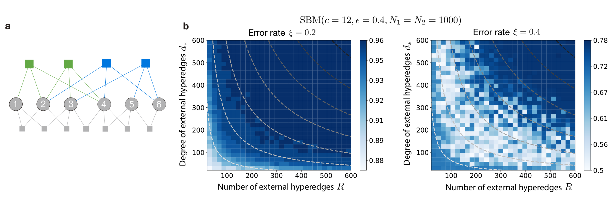
Figure 7: Numerical experiments regarding spectral clustering on the symmetric SBM with noisy external hyperedges. (a) A schematic of the scotch-taping we consider, and (b) the density plots of the accuracy values for various numbers of external hyperedges RR (horizontal axis) and the degree of each external hyperedge d∗d_{\ast} (vertical axis). We used the same graph instance of the SBM as in Fig. 3. The error rate of the noisy external hyperedges is represented by ξ\xi. The dashed curves indicate the parameter pairs for which the total number (represented by the color depth) of edges among the external hyperedges is preserved.

We assume that an annotation label is shared by a large number of physical nodes. In previous sections, we considered scotch-taping such that each factor node is connected to all these physical nodes. However, a division into several external hyperedges with small degree may be more beneficial. We consider this problem in this section.

In fact, neither of these strategies has a general benefit or drawback. As mentioned above, the terms relevant to the external hyperedges are 2​N​∑rhr​mr/drv2N\sum_{r}h^{r}m_{r}/d^{v}_{r} and ∑r=1Rhr\sum_{r=1}^{R}h^{r}. The term 2​N​∑rhr​mr/drv2N\sum_{r}h^{r}m_{r}/d^{v}_{r} in the message-passing equation (24) is always O⁡(1)O(1) or less; in order that hr​mrh^{r}m_{r} be O⁡(1)O(1), the degree drvd^{v}_{r} should be O⁡(N)O(N), whereas hr​mrh^{r}m_{r} can be at most O⁡(1/N)O(1/N) when drvd^{v}_{r} is O⁡(1)O(1). Thus, dividing an external hyperedge into multiple hyperedges with small degree does not necessarily strengthen or weaken its contribution.

The contribution from ∑r=1Rhr\sum_{r=1}^{R}h^{r} is also preserved as long as the total number of external edges remains the same. For example, let us assume that we originally have two external hyperedges corresponding to groups 1 and 2, and node i∈Ui\in U is incident to the external hyperedge corresponding to group 1; then, we would have (hi1,hi2)=(1,0)(h^{1}_{i},h^{2}_{i})=(1,0), which is the iith row in the HH matrix in Eq. (1). If we divide the external hyperedge corresponding to group 1 into two, then we would have (hi(1,1),hi(1,2),hi2)(h^{(1,1)}_{i},h^{(1,2)}_{i},h^{2}_{i}) that is equal to either (1,0,0)(1,0,0) or (0,1,0)(0,1,0). In all cases, we have ∑r=1Rhir=1\sum_{r=1}^{R}h^{r}_{i}=1. This demonstrates that the statistic of ∑r=1Rhr\sum_{r=1}^{R}h^{r} is invariant under the divisions of external hyperedges.

We further confirm that there is no clear benefit between few external hyperedges with large degrees and many external hyperedges with small degrees through a numerical experiment. In this experiment, we consider noisy external hyperedges of Type 2 with error rate ξ\xi, as schematically shown in Fig. 7a. That is, we add R/2R/2 external hyperedges to increase the density in group 1, and R/2R/2 external hyperedges to increase the density in group 2. Among drv=d∗(const.)d^{v}_{r}=d_{\ast}\,(\mathrm{const.}) edges incident to an external hyperedge of the first half, edges are randomly connected to the physical nodes in group 1 with probability 1−ξ1-\xi, and the rest are randomly connected to the physical nodes in group 2. Similarly, for an external hyperedge of the second half, edges are randomly connected to the physical nodes in group 2 with probability 1−ξ1-\xi, and the rest are randomly connected to the physical nodes in group 1.

Each panel in Fig. 7b shows the accuracy regarding the planted group assignments of the symmetric SBM as the number of external hyperedges (horizontal axis) and the degree of each external hyperedge (vertical axis) vary. The dashed curves represent the parameter pairs for which d∗​Rd_{\ast}R is conserved. Evidently, the accuracy is the same on each dashed curve, implying that there is no preference in the balance between the number of external hyperedges RR and the degree of each external hyperedge d∗d_{\ast}. Interestingly, it is also confirmed from the right panel of Fig. 7b that the accuracy improvement by scotch-taping can be nonmonotonic. Therefore, depending on the values of ϵ\epsilon and ξ\xi, there exists an intermediate range in the (d∗,R)(d_{\ast},R) space where the external hyperedges act as noise even though this scotch-taping eventually improves the accuracy when we add more external hyperedges.

VII Discussion

We considered a simple method to encode node annotations on a graph as a factor graph, and we established the mathematical basis of the method in the spectral framework. Even though scotch-taping may be used in various inference problems, we focused on the inference of an assortative module structure.

As mentioned in Sec. II, because scotch-taping is based only on the data representation, it can be combined with an arbitrary algorithm on graphs. Non-negative matrix factorization (NMF) Lee and Seung 1999 is a method similar to spectral clustering, and in Appendix E, we present applications of NMF to the scotch-taped incidence matrix BB. A numerical experiment in Appendix E demonstrates that, even a few uniform external hyperedges disrupt the inference of the module structure of the original graph, indicating that the observed behavior regarding spectral clustering in Secs. V.1 and VI.1 is not universal.

Scotch-taped graphs can be used as input to nonlinear graph embedding methods, such as DeepWalk Perozzi et al. 2014, node2vec Grover and Leskovec 2016, and LINE Tang et al. 2015. The fact that these methods can only take a graph as input is occasionally characterized as their fundamental limitation Hamilton et al. 2017b. However, scotch-taping naturally extends the applicability of these embedding methods.

The graph convolutional network (GCN) Kipf and Welling 2016 is a popular GNN algorithm. Although the GCN already considers node annotations (or features) as well as the graph structure, it is also possible to use a scotch-taped graph as input. The original GCN uses (monopartite) graphs; however, we can immediately generalize it to factor graphs (bipartite graphs) by considering the following variant of the feed-forward architecture of the GCN:

Xt+1=σ^​(𝖡​σ^​(𝖡⊤​Xt​WUt)​WVt),\displaystyle X^{t+1}=\hat{\sigma}\left(\mathsf{B}\,\hat{\sigma}\left(\mathsf{B}^{\top}X^{t}W_{U}^{t}\right)W_{V}^{t}\right), (30)

where t∈{0,1,…,T}t\in\{0,1,\dots,T\} represents the layer index, and σ^\hat{\sigma} is a nonlinear operator. Xt∈ℝN×RUtX^{t}\in\mathbb{R}^{N\times R^{t}_{U}} is the feature matrix of the physical nodes (X0=HX^{0}=H), which is to be updated across the layers. WUtW_{U}^{t} and WVtW_{V}^{t} are linear transforms at the ttth layer that are to be learned. Equation (30) has the potential to encode richer information because two different types of node attributes can be inserted into X0X^{0} and 𝖡\mathsf{B}, respectively. We empirically confirmed that scotch-taping can both improve and deteriorate prediction in nonlinear graph embedding methods and GCN, depending on the dataset.

Let us finally consider some qualitative distinctions between the inference using a scotch-taped graph and other popular methods. In Bayesian inference Newman and Clauset 2016; Hric et al. 2016, graph data and node annotations interact indirectly in a generative model, because the former contributes to a likelihood whereas the latter does to a prior. In contrast, scotch-taping treats both graph data and node annotations on an equal footing; thus, they interact more directly. Similarly, in the GCN framework, the contribution of node attributes in the feature matrix in X0X^{0} is different from that in the incidence matrix 𝖡\mathsf{B}.

What scotch-taping suggests is why don’t you simply add edges if you believe a set of nodes are similar or dissimilar to each other?. This is simplistic and may even appear ad hoc. However, it is certainly a choice when other sophisticated methods fail. In real data analysis, it is conceivable that several practitioners have used a technique similar to scotch-taping. In any case, we can always consider using scotch-taping to further improve the performance of an algorithm, or to determine whether node annotations are consistent with the underlying graph structure.

Acknowledgements.
This study was partly supported by the New Energy and Industrial Technology Development Organization (NEDO) and JSPS KAKENHI No. 18K18604.

Appendix A Brillouin–Wigner expansion

In the main text, we obtained a formal solution of the generalized eigenvalue equation (6) using an expansion in the form the Lippmann–Schwinger equation. Here, we show that another formal solution can be obtained by using the Brillouin–Wigner expansion Ziman 1969.

Equation (6) with respect to the kkth eigenvalue λk=2​sk2\lambda_{k}=2s^{2}_{k} is the following eigenvalue equation:

2​𝖡𝖡⊤​ϕk′\displaystyle 2\mathsf{B}\mathsf{B}^{\top}\mbox{\boldmath$\phi$}^{\prime}_{k} =λk​ϕk′.\displaystyle=\lambda_{k}\mbox{\boldmath$\phi$}^{\prime}_{k}. (31)

We note that the matrix on the left-hand side is

2𝖡𝖡⊤=ℋ′=D−1/2UℋD−1/2U,\displaystyle 2\mathsf{B}\mathsf{B}^{\top}=\mathcal{H}^{\prime}=D^{-1/2}_{U}\mathcal{H}D^{-1/2}_{U}, (32)
ℋ≡−L+2​DU0+2​∑r𝒉r​𝒉r⊤drv.\displaystyle\mathcal{H}\equiv-L+2D^{0}_{U}+2\sum_{r}\frac{\mbox{\boldmath$h$}^{r}\mbox{\boldmath$h$}^{r\top}}{d^{v}_{r}}. (33)

In the absence of external hyperedges, we let

ℋ0′=DU0−1/2​ℋ0​DU0−1/2,ℋ0≡−L+2​DU0,\displaystyle\mathcal{H}^{\prime}_{0}=D^{0\,-1/2}_{U}\mathcal{H}_{0}D^{0\,-1/2}_{U},\hskip 20.0pt\mathcal{H}_{0}\equiv-L+2D^{0}_{U}, (34)

and we define ℋ~′≡ℋ′−ℋ0′\widetilde{\mathcal{H}}^{\prime}\equiv\mathcal{H}^{\prime}-\mathcal{H}^{\prime}_{0}.

The eigenvalue equation (31) is then reformulated as

(λk−ℋ0′)​ϕk′=ℋ~′​ϕk′\displaystyle\left(\lambda_{k}-\mathcal{H}^{\prime}_{0}\right)\mbox{\boldmath$\phi$}^{\prime}_{k}=\widetilde{\mathcal{H}}^{\prime}\mbox{\boldmath$\phi$}^{\prime}_{k} (35)

In the Brillouin–Wigner expansion, we consider the following projection operators:

Π≡𝝋k′​𝝋k′⁣⊤,Θ≡I−Π,\displaystyle\Pi\equiv\mbox{\boldmath$\varphi$}^{\prime}_{k}\mbox{\boldmath$\varphi$}^{\prime\top}_{k},\hskip 20.0pt\Theta\equiv I-\Pi, (36)

where 𝝋k′\mbox{\boldmath$\varphi$}^{\prime}_{k} (=DU0 1/2​𝝋k=D^{0\,1/2}_{U}\mbox{\boldmath$\varphi$}_{k}) is the kkth eigenvector of ℋ0′\mathcal{H}^{\prime}_{0}. In addition, ignoring the normalization of ϕk′\mbox{\boldmath$\phi$}^{\prime}_{k}, we introduce a residual 𝜻k\mbox{\boldmath$\zeta$}_{k} vector such that

ϕk′=𝝋k′+𝜻k,𝜻k⊤​𝝋k′=0.\displaystyle\mbox{\boldmath$\phi$}^{\prime}_{k}=\mbox{\boldmath$\varphi$}^{\prime}_{k}+\mbox{\boldmath$\zeta$}_{k},\hskip 20.0pt\mbox{\boldmath$\zeta$}^{\top}_{k}\mbox{\boldmath$\varphi$}^{\prime}_{k}=0. (37)

By applying Θ\Theta from the left on the both sides of Eq. (35), we have

Θ⁡(λk−ℋ0′)​(𝝋k′+𝜻k)\displaystyle\Theta\left(\lambda_{k}-\mathcal{H}^{\prime}_{0}\right)\left(\mbox{\boldmath$\varphi$}^{\prime}_{k}+\mbox{\boldmath$\zeta$}_{k}\right) =Θ​ℋ~′​ϕk′\displaystyle=\Theta\widetilde{\mathcal{H}}^{\prime}\mbox{\boldmath$\phi$}^{\prime}_{k}
(λk−λk0)​Θ​𝝋k′+(λk−ℋ0′)​Θ​𝜻k\displaystyle\left(\lambda_{k}-\lambda^{0}_{k}\right)\Theta\mbox{\boldmath$\varphi$}^{\prime}_{k}+\left(\lambda_{k}-\mathcal{H}^{\prime}_{0}\right)\Theta\mbox{\boldmath$\zeta$}_{k} =Θ​ℋ~′​ϕk′\displaystyle=\Theta\widetilde{\mathcal{H}}^{\prime}\mbox{\boldmath$\phi$}^{\prime}_{k}
(λk−ℋ0′)​𝜻k\displaystyle\left(\lambda_{k}-\mathcal{H}^{\prime}_{0}\right)\mbox{\boldmath$\zeta$}_{k} =Θ​ℋ~′​ϕk′\displaystyle=\Theta\widetilde{\mathcal{H}}^{\prime}\mbox{\boldmath$\phi$}^{\prime}_{k}
𝜻k\displaystyle\mbox{\boldmath$\zeta$}_{k} =(λk−ℋ0′)−1​Θ​ℋ~′​ϕk′.\displaystyle=\left(\lambda_{k}-\mathcal{H}^{\prime}_{0}\right)^{-1}\Theta\widetilde{\mathcal{H}}^{\prime}\mbox{\boldmath$\phi$}^{\prime}_{k}. (38)

In the second line, we used ℋ0′​𝝋k′=λk0​𝝋k′\mathcal{H}^{\prime}_{0}\mbox{\boldmath$\varphi$}^{\prime}_{k}=\lambda^{0}_{k}\mbox{\boldmath$\varphi$}^{\prime}_{k} and Θ​ℋ0′​𝜻k=ℋ0′​Θ​𝜻k\Theta\mathcal{H}^{\prime}_{0}\mbox{\boldmath$\zeta$}_{k}=\mathcal{H}^{\prime}_{0}\Theta\mbox{\boldmath$\zeta$}_{k} (because 𝜻k⊤​𝝋k′=0\mbox{\boldmath$\zeta$}^{\top}_{k}\mbox{\boldmath$\varphi$}^{\prime}_{k}=0). In the third line, we used Θ​𝝋k′=𝟎\Theta\mbox{\boldmath$\varphi$}^{\prime}_{k}=\mbox{\boldmath$0$} and Θ​𝜻k=𝜻k\Theta\mbox{\boldmath$\zeta$}_{k}=\mbox{\boldmath$\zeta$}_{k}. In the fourth line, we defined (λk−ℋ0′)−1\left(\lambda_{k}-\mathcal{H}^{\prime}_{0}\right)^{-1} as the inverse of (λk−ℋ0′)\left(\lambda_{k}-\mathcal{H}^{\prime}_{0}\right). By substituting Eq. (38) into the first equation in Eq. (37), we have

ϕk′\displaystyle\mbox{\boldmath$\phi$}^{\prime}_{k} =𝝋k′+(λk−ℋ0′)−1​Θ​ℋ~′​ϕk′\displaystyle=\mbox{\boldmath$\varphi$}^{\prime}_{k}+\left(\lambda_{k}-\mathcal{H}^{\prime}_{0}\right)^{-1}\Theta\widetilde{\mathcal{H}}^{\prime}\mbox{\boldmath$\phi$}^{\prime}_{k}
=𝝋k′+(λk−ℋ0′)−1​Θ​ℋ~′​𝝋k′\displaystyle=\mbox{\boldmath$\varphi$}^{\prime}_{k}+\left(\lambda_{k}-\mathcal{H}^{\prime}_{0}\right)^{-1}\Theta\widetilde{\mathcal{H}}^{\prime}\mbox{\boldmath$\varphi$}^{\prime}_{k}
+(λk−ℋ0′)−1​Θ​ℋ~′​(λk−ℋ0′)−1​Θ​ℋ~′​𝝋k′+⋯.\displaystyle\hskip 10.0pt+\left(\lambda_{k}-\mathcal{H}^{\prime}_{0}\right)^{-1}\Theta\widetilde{\mathcal{H}}^{\prime}\left(\lambda_{k}-\mathcal{H}^{\prime}_{0}\right)^{-1}\Theta\widetilde{\mathcal{H}}^{\prime}\mbox{\boldmath$\varphi$}^{\prime}_{k}+\cdots. (39)

This formal solution is known as the Brillouin–Wigner expansion. Although this is similar to Eq. (9), Eq. (39) is written in terms of the regularized vectors 𝝋k′\mbox{\boldmath$\varphi$}^{\prime}_{k} and ϕk′\mbox{\boldmath$\phi$}^{\prime}_{k}. We note that both Eqs. (9) and (39) require λk\lambda_{k} as well as λk0\lambda^{0}_{k}.

Appendix B Derivation of the eigenvalue equation in the crude approximation

B.1 Original graph

In the absence of external hyperedges, the generalized eigenvalue equation (6) is approximated as

∑j∈UAi​j​φk​j\displaystyle\sum_{j\in U}A_{ij}\varphi_{kj} =(λk0−1)​diu​φk​i,\displaystyle=(\lambda^{0}_{k}-1)d^{u}_{i}\varphi_{ki},
1Nσ​∑i∈Uσ∑j∈UAi​j​φk​j\displaystyle\frac{1}{N_{\sigma}}\sum_{i\in U_{\sigma}}\sum_{j\in U}A_{ij}\varphi_{kj} =λk0−1Nσ​∑i∈Uσdiu​φk​i≈(λk0−1)​cσ​φ¯k​σ.\displaystyle=\frac{\lambda^{0}_{k}-1}{N_{\sigma}}\sum_{i\in U_{\sigma}}d^{u}_{i}\varphi_{ki}\approx(\lambda^{0}_{k}-1)c_{\sigma}\bar{\varphi}_{k\sigma}. (40)

The left-hand side is approximated as

1Nσ​∑i∈Uσ∑j∈UAi​j​φk​j\displaystyle\frac{1}{N_{\sigma}}\sum_{i\in U_{\sigma}}\sum_{j\in U}A_{ij}\varphi_{kj} ≈1Nσ​∑σ′(∑i∈Uσ∑j∈Uσ′Ai​j)​φ¯k​σ′\displaystyle\approx\frac{1}{N_{\sigma}}\sum_{\sigma^{\prime}}\left(\sum_{i\in U_{\sigma}}\sum_{j\in U_{\sigma^{\prime}}}A_{ij}\right)\bar{\varphi}_{k\sigma^{\prime}}
=1Nσ​∑σ′(1+δ⁡(σ,σ′))​eσ​σ′​φ¯k​σ′\displaystyle=\frac{1}{N_{\sigma}}\sum_{\sigma^{\prime}}\left(1+\delta(\sigma,\sigma^{\prime})\right)e_{\sigma\sigma^{\prime}}\bar{\varphi}_{k\sigma^{\prime}}
=cσ​∑σ′fσ​σ′​φ¯k​σ′.\displaystyle=c_{\sigma}\sum_{\sigma^{\prime}}f_{\sigma\sigma^{\prime}}\bar{\varphi}_{k\sigma^{\prime}}. (41)

Then, we obtain the approximated generalized eigenvalue equation (11) in the main text.

B.2 Scotch-taped graph

In the presence of external hyperedges, the element-wise expression of the generalized eigenvalue equation (6) is

∑j∈U(Ai​j+2​∑rhir​hjrdrv)​ϕk​j=(diu​(λk−1)+λk​∑rhir)​ϕk​i.\displaystyle\sum_{j\in U}\left(A_{ij}+2\sum_{r}\frac{h^{r}_{i}h^{r}_{j}}{d^{v}_{r}}\right)\phi_{kj}=\left(d^{u}_{i}(\lambda_{k}-1)+\lambda_{k}\sum_{r}h^{r}_{i}\right)\phi_{ki}. (42)

By the definition of hσr¯\overline{h^{r}_{\sigma}},

1Nσ​∑i∈Uσ∑j∈U2​∑rhir​hjrdrv​ϕk​j\displaystyle\frac{1}{N_{\sigma}}\sum_{i\in U_{\sigma}}\sum_{j\in U}2\sum_{r}\frac{h^{r}_{i}h^{r}_{j}}{d^{v}_{r}}\phi_{kj}
=2​∑rhσr¯∑σ′′hσ′′r¯​Nσ′′​∑j∈Uhjr​ϕk​j\displaystyle\hskip 10.0pt=2\sum_{r}\frac{\overline{h^{r}_{\sigma}}}{\sum_{\sigma^{\prime\prime}}\overline{h^{r}_{\sigma^{\prime\prime}}}N_{\sigma^{\prime\prime}}}\sum_{j\in U}h^{r}_{j}\phi_{kj}
≈2​∑rhσr¯∑σ′′hσ′′r¯​Nσ′′​∑σ′hσ′r¯​Nσ′​ϕk​σ′.\displaystyle\hskip 10.0pt\approx 2\sum_{r}\frac{\overline{h^{r}_{\sigma}}}{\sum_{\sigma^{\prime\prime}}\overline{h^{r}_{\sigma^{\prime\prime}}}N_{\sigma^{\prime\prime}}}\sum_{\sigma^{\prime}}\overline{h^{r}_{\sigma^{\prime}}}N_{\sigma^{\prime}}\phi_{k\sigma^{\prime}}. (43)

Here, we used drv=∑σ′′hσ′′r¯​Nσ′′d^{v}_{r}=\sum_{\sigma^{\prime\prime}}\overline{h^{r}_{\sigma^{\prime\prime}}}N_{\sigma^{\prime\prime}}. Using Eqs. (40), (41), and (43), Eq. (42) is approximated as Eq. (12) in the main text.

Appendix C Replica method

In this section, we derive the message-passing equation of the second-largest eigenvector-element distribution for the microcanonical SBM. Equation (90) corresponds to Eq. (24) in the main text; AQA_{Q} and HQH_{Q} in Eq. (90) are replaced by 𝖠\mathsf{A} and 𝖧\mathsf{H} in Eq. (24) in the main text, respectively.

To calculate [λ2]B0\left[\lambda_{2}\right]_{B^{0}} in Eq. (21), we should calculate the moment [Zn​(β,λ,γ)]B0\left[Z^{n}(\beta,\lambda,\gamma)\right]_{B^{0}}. According to Eqs. (19) and (20), the nnth power of Zn​(β,μ,λ,γ)Z^{n}(\beta,\mu,\lambda,\gamma) is

Zn​(β,μ,λ,γ)\displaystyle Z^{n}(\beta,\mu,\lambda,\gamma) =∫∏i∈U∏a=1nd​xi​a​exp⁡(β​∑a=1n(12​λ​N+12​(∑i∈Uxi​a​Bi​α0)2+∑r=1R1drv​(∑i∈Uxi​a​hir)2CLOSECLOSE\displaystyle=\int\prod_{i\in U}\prod_{a=1}^{n}dx_{ia}\,\exp\Biggl(\beta\sum_{a=1}^{n}\biggl(\frac{1}{2}\lambda N+\frac{1}{2}\left(\sum_{i\in U}x_{ia}B^{0}_{i\alpha}\right)^{2}+\sum_{r=1}^{R}\frac{1}{d^{v}_{r}}\left(\sum_{i\in U}x_{ia}h^{r}_{i}\right)^{2}
−λ2∑i∈Udiuxi​a2−γ∑i∈Udiuxi​a)).\displaystyle\hskip 100.0pt-\frac{\lambda}{2}\sum_{i\in U}d^{u}_{i}x^{2}_{ia}-\gamma\sum_{i\in U}d^{u}_{i}x_{ia}\biggr)\Biggr). (44)

By introducing the auxiliary variables

yα​a=∑i∈Uxi​a​Bi​α0,(α∈V0)\displaystyle y_{\alpha a}=\sum_{i\in U}x_{ia}B^{0}_{i\alpha},\hskip 10.0pt(\alpha\in V^{0}) (45)
mr​a=1N​∑i∈Uxi​a​hir,\displaystyle m_{ra}=\frac{1}{N}\sum_{i\in U}x_{ia}h^{r}_{i}, (46)

we have

Zn​(β,λ,γ)\displaystyle Z^{n}(\beta,\lambda,\gamma) =∫∏i,ad​xi​a​∫∏α,ad​yα​a​∫∏r,ad​mr​a​∏α∈V0δ⁡(yα​a−∑i∈Uxi​a​Bi​α0)​∏α∈V0δ⁡(mr​a−1N​∑i∈Uxi​a​hir)\displaystyle=\int\prod_{i,a}dx_{ia}\,\int\prod_{\alpha,a}dy_{\alpha a}\int\prod_{r,a}dm_{ra}\prod_{\alpha\in V^{0}}\delta\left(y_{\alpha a}-\sum_{i\in U}x_{ia}B^{0}_{i\alpha}\right)\prod_{\alpha\in V^{0}}\delta\left(m_{ra}-\frac{1}{N}\sum_{i\in U}x_{ia}h^{r}_{i}\right)
×exp⁡(12​n​β​λ​N+β2​∑a=1n∑α∈V0yα​a2+β​N2​∑a=1n∑r=1R1drv​mr​a2−β​∑a=1n∑i∈Udiu​(λ2​xi​a2+γ​xi​a))\displaystyle\times\exp\Biggl(\frac{1}{2}n\beta\lambda N+\frac{\beta}{2}\sum_{a=1}^{n}\sum_{\alpha\in V^{0}}y_{\alpha a}^{2}+\beta N^{2}\sum_{a=1}^{n}\sum_{r=1}^{R}\frac{1}{d^{v}_{r}}m_{ra}^{2}-\beta\sum_{a=1}^{n}\sum_{i\in U}d^{u}_{i}(\frac{\lambda}{2}x^{2}_{ia}+\gamma x_{ia})\Biggr) (47)
=∫∏i,ad​xi​a​∫∏α,ad​y^α​a​d​yα​a2​π​∫∏r,aβ​N​d​m^r​a​d​mr​a2​π\displaystyle=\int\prod_{i,a}dx_{ia}\,\int\prod_{\alpha,a}\frac{d\hat{y}_{\alpha a}dy_{\alpha a}}{2\pi}\int\prod_{r,a}\frac{\beta Nd\hat{m}_{ra}dm_{ra}}{2\pi}
×exp⁡(12​n​β​λ​N+β2​∑a=1n∑α∈V0yα​a2+β​N2​∑a=1n∑r=1R1drv​mr​a2CLOSE\displaystyle\times\exp\Biggl(\frac{1}{2}n\beta\lambda N+\frac{\beta}{2}\sum_{a=1}^{n}\sum_{\alpha\in V^{0}}y_{\alpha a}^{2}+\beta N^{2}\sum_{a=1}^{n}\sum_{r=1}^{R}\frac{1}{d^{v}_{r}}m_{ra}^{2}
−β∑a=1n∑i∈U∑α∈V0Bi​α0(λ2xi​a2+γxi​a)−β∑a=1n∑i∈U∑rhir(λ2xi​a2+γxi​a)\displaystyle-\beta\sum_{a=1}^{n}\sum_{i\in U}\sum_{\alpha\in V_{0}}B^{0}_{i\alpha}(\frac{\lambda}{2}x^{2}_{ia}+\gamma x_{ia})-\beta\sum_{a=1}^{n}\sum_{i\in U}\sum_{r}h^{r}_{i}(\frac{\lambda}{2}x^{2}_{ia}+\gamma x_{ia})
−β∑a∑α∈V0y^α​a(yα​a−∑i∈Uxi​aBi​α0)−β∑a∑rm^r​a(mr​aN−∑i∈Uxi​ahir)).\displaystyle-\beta\sum_{a}\sum_{\alpha\in V^{0}}\hat{y}_{\alpha a}\left(y_{\alpha a}-\sum_{i\in U}x_{ia}B^{0}_{i\alpha}\right)-\beta\sum_{a}\sum_{r}\hat{m}_{ra}\left(m_{ra}N-\sum_{i\in U}x_{ia}h^{r}_{i}\right)\Biggr). (48)

Here, we used the fact that the degree diud^{u}_{i} of a physical node is decomposed as diu=∑α∈V0Bi​α0+∑rhird^{u}_{i}=\sum_{\alpha\in V_{0}}B^{0}_{i\alpha}+\sum_{r}h^{r}_{i}. Then, the moment can be calculated as follows:

[Zn​(β,λ,γ)]B0\displaystyle\left[Z^{n}(\beta,\lambda,\gamma)\right]_{B^{0}}
=∫∏i,ad​xi​a​∫∏α,ad​y^α​a​d​yα​a2​π​∫∏r,aβ​N​d​m^r​a​d​mr​a2​π​exp⁡(12​n​β​λ​N−β​∑a=1n∑i∈U∑rhir​(λ2​xi​a2+γ​xi​a)CLOSE\displaystyle=\int\prod_{i,a}dx_{ia}\,\int\prod_{\alpha,a}\frac{d\hat{y}_{\alpha a}dy_{\alpha a}}{2\pi}\int\prod_{r,a}\frac{\beta Nd\hat{m}_{ra}dm_{ra}}{2\pi}\,\exp\Biggl(\frac{1}{2}n\beta\lambda N-\beta\sum_{a=1}^{n}\sum_{i\in U}\sum_{r}h^{r}_{i}(\frac{\lambda}{2}x^{2}_{ia}+\gamma x_{ia})
+β2∑a=1n∑α∈V0(yα​a2−2y^α​ayα​a)+βN∑a=1n∑r=1R(Ndrvmr​a2−m^r​amr​a)+β∑a∑i∈U∑rm^r​axi​ahir)\displaystyle\hskip 20.0pt+\frac{\beta}{2}\sum_{a=1}^{n}\sum_{\alpha\in V^{0}}\left(y_{\alpha a}^{2}-2\hat{y}_{\alpha a}y_{\alpha a}\right)+\beta N\sum_{a=1}^{n}\sum_{r=1}^{R}\left(\frac{N}{d^{v}_{r}}m_{ra}^{2}-\hat{m}_{ra}m_{ra}\right)+\beta\sum_{a}\sum_{i\in U}\sum_{r}\hat{m}_{ra}x_{ia}h^{r}_{i}\Biggr)
×[exp(−β∑a∑α∈V0∑i∈UBi​α0(λ2xi​a2+γxi​a−xi​ay^α​a))]B0.\displaystyle\hskip 20.0pt\times\left[\exp\left(-\beta\sum_{a}\sum_{\alpha\in V^{0}}\sum_{i\in U}B^{0}_{i\alpha}(\frac{\lambda}{2}x^{2}_{ia}+\gamma x_{ia}-x_{ia}\hat{y}_{\alpha a})\right)\right]_{B^{0}}. (49)

By using the probability distribution of the microcanonical SBM (Eq. (10)), the last factor is calculated as

[exp(−β∑a∑α∈V0∑i∈UBi​α0(λ2xi​a2+γxi​a−xi​ay^α​a))]B0\displaystyle\left[\exp\left(-\beta\sum_{a}\sum_{\alpha\in V^{0}}\sum_{i\in U}B^{0}_{i\alpha}(\frac{\lambda}{2}x^{2}_{ia}+\gamma x_{ia}-x_{ia}\hat{y}_{\alpha a})\right)\right]_{B^{0}}
=1𝒩G​∑{Bi​α0}∏σ∏α∈Vσ​σδ⁡(∑i∈UσBi​α0,2)​∏σ<σ′∏α∈Vσ​σ′0δ⁡(∑i∈UσBi​α0,1)​δ​(∑j∈Uσ′Bj​α0,1)\displaystyle=\frac{1}{\mathcal{N}_{G}}\sum_{\{B^{0}_{i\alpha}\}}\prod_{\sigma}\prod_{\alpha\in V_{\sigma\sigma}}\delta\left(\sum_{i\in U_{\sigma}}B^{0}_{i\alpha},2\right)\prod_{\sigma<\sigma^{\prime}}\prod_{\alpha\in V^{0}_{\sigma\sigma^{\prime}}}\delta\left(\sum_{i\in U_{\sigma}}B^{0}_{i\alpha},1\right)\delta\left(\sum_{j\in U_{\sigma^{\prime}}}B^{0}_{j\alpha},1\right)
×∏α∈V0exp(−β∑a∑i∈UBi​α0(λ2xi​a2+γxi​a−xi​ay^α​a))\displaystyle\hskip 80.0pt\times\prod_{\alpha\in V^{0}}\exp\left(-\beta\sum_{a}\sum_{i\in U}B^{0}_{i\alpha}(\frac{\lambda}{2}x^{2}_{ia}+\gamma x_{ia}-x_{ia}\hat{y}_{\alpha a})\right) (50)
=1𝒩G​∑{Bi​α0}∮∏σ=1K∏α∈Vσ​σ0d​zα​σ2​π​i​zα​σ(1−∑i∈UσBi​α0)\displaystyle=\frac{1}{\mathcal{N}_{G}}\sum_{\{B^{0}_{i\alpha}\}}\oint\prod_{\sigma=1}^{K}\prod_{\alpha\in V^{0}_{\sigma\sigma}}\frac{dz_{\alpha\sigma}}{2\pi i}z_{\alpha\sigma}^{(1-\sum_{i\in U_{\sigma}}B^{0}_{i\alpha})}
×∮∏σ<σ′∏α∈Vσ​σ′0d​zα​σ2​π​id​zα​σ′2​π​izα−∑i∈UσB0i​αzα−∑j∈Uσ′B0j​α\displaystyle\hskip 40.0pt\times\oint\prod_{\sigma<\sigma^{\prime}}\prod_{\alpha\in V^{0}_{\sigma\sigma^{\prime}}}\frac{dz_{\alpha\sigma}}{2\pi i}\frac{dz_{\alpha\sigma^{\prime}}}{2\pi i}z_{\alpha}^{-\sum_{i\in U_{\sigma}}B^{0}_{i\alpha}}z_{\alpha}^{-\sum_{j\in U_{\sigma^{\prime}}}B^{0}_{j\alpha}}
×∏α∈V0exp(−β∑a∑i∈UBi​α0(λ2xi​a2+γxi​a−xi​ay^α​a))\displaystyle\hskip 40.0pt\times\prod_{\alpha\in V^{0}}\exp\left(-\beta\sum_{a}\sum_{i\in U}B^{0}_{i\alpha}(\frac{\lambda}{2}x^{2}_{ia}+\gamma x_{ia}-x_{ia}\hat{y}_{\alpha a})\right) (51)
=1𝒩G∏σ=1K(∑{Bi​α0}α∈Vσ​σ0i∈Uσ∮∏α∈Vσ​σ0(d​zα​σ2​π​izα​σ∏i∈Uσzα​σ−Bi​α0∏i∈Uσe−β∑aB0i​α(λ2x2i​a+γxi​a−xi​ay^α​a)))\displaystyle=\frac{1}{\mathcal{N}_{G}}\prod_{\sigma=1}^{K}\left(\sum_{\{B^{0}_{i\alpha}\}^{i\in U_{\sigma}}_{\alpha\in V^{0}_{\sigma\sigma}}}\oint\prod_{\alpha\in V^{0}_{\sigma\sigma}}\left(\frac{dz_{\alpha\sigma}}{2\pi i}z_{\alpha\sigma}\prod_{i\in U_{\sigma}}z_{\alpha\sigma}^{-B^{0}_{i\alpha}}\prod_{i\in U_{\sigma}}\mathrm{e}^{-\beta\sum_{a}B^{0}_{i\alpha}(\frac{\lambda}{2}x^{2}_{ia}+\gamma x_{ia}-x_{ia}\hat{y}_{\alpha a})}\right)\right)
×∏σ<σ′K(∑{Bi​α0}α∈Vσ​σ′0i∈Uσ∪Uσ′∮∏α∈Vσ​σ′0(d​zα​σ​d​zα​σ′(2​π​i)2∏i∈Uσzα​σ−Bi​α0∏j∈Uσ′zα​σ′−Bj​α0∏i∈Uσ∪Uσ′e−β∑aB0i​α(λ2x2i​a+γxi​a−xi​ay^α​a))).\displaystyle\times\prod_{\sigma<\sigma^{\prime}}^{K}\left(\sum_{\{B^{0}_{i\alpha}\}^{i\in U_{\sigma}\cup U_{\sigma^{\prime}}}_{\alpha\in V^{0}_{\sigma\sigma^{\prime}}}}\oint\prod_{\alpha\in V^{0}_{\sigma\sigma^{\prime}}}\left(\frac{dz_{\alpha\sigma}dz_{\alpha\sigma^{\prime}}}{(2\pi i)^{2}}\prod_{i\in U_{\sigma}}z_{\alpha\sigma}^{-B^{0}_{i\alpha}}\prod_{j\in U_{\sigma^{\prime}}}z_{\alpha\sigma^{\prime}}^{-B^{0}_{j\alpha}}\prod_{i\in U_{\sigma}\cup U_{\sigma^{\prime}}}\mathrm{e}^{-\beta\sum_{a}B^{0}_{i\alpha}(\frac{\lambda}{2}x^{2}_{ia}+\gamma x_{ia}-x_{ia}\hat{y}_{\alpha a})}\right)\right). (52)

Here, we introduce the following order-parameter functions:

Qσ​(𝘅)≡1Nσ​∑i∈Uσ∏a=1nδ⁡(𝗑a−xi​a),\displaystyle Q_{\sigma}(\mbox{\boldmath$\mathsf{x}$})\equiv\frac{1}{N_{\sigma}}\sum_{i\in U_{\sigma}}\prod_{a=1}^{n}\delta\left(\mathsf{x}_{a}-x_{ia}\right), (53)
Pσ​σ′​(𝘆)≡1eσ​σ′​∑α∈Vσ​σ′0zα​σ−1​∏a=1nδ⁡(𝗒a−y^α​a).\displaystyle P_{\sigma\sigma^{\prime}}(\mbox{\boldmath$\mathsf{y}$})\equiv\frac{1}{e_{\sigma\sigma^{\prime}}}\sum_{\alpha\in V^{0}_{\sigma\sigma^{\prime}}}z_{\alpha\sigma}^{-1}\prod_{a=1}^{n}\delta\left(\mathsf{y}_{a}-\hat{y}_{\alpha a}\right). (54)

Pσ​σ′​(𝘆)P_{\sigma\sigma^{\prime}}(\mbox{\boldmath$\mathsf{y}$}) is asymmetric with respect to σ\sigma and σ′\sigma^{\prime}, and it is order-sensitive. By using Qσ​(𝘅)Q_{\sigma}(\mbox{\boldmath$\mathsf{x}$}) and Pσ​σ′​(𝘆)P_{\sigma\sigma^{\prime}}(\mbox{\boldmath$\mathsf{y}$}), for the factor of Vσ​σ0V^{0}_{\sigma\sigma},

∑{Bi​α0}α∈Vσ​σ0i∈Uσ∮∏α∈Vσ​σ0(d​zα​σ2​π​izα​σ∏i∈Uσzα​σ−Bi​α0∏i∈Uσe−β∑aB0i​α(λ2x2i​a+γxi​a−xi​ay^α​a))\displaystyle\sum_{\{B^{0}_{i\alpha}\}^{i\in U_{\sigma}}_{\alpha\in V^{0}_{\sigma\sigma}}}\oint\prod_{\alpha\in V^{0}_{\sigma\sigma}}\left(\frac{dz_{\alpha\sigma}}{2\pi i}z_{\alpha\sigma}\prod_{i\in U_{\sigma}}z_{\alpha\sigma}^{-B^{0}_{i\alpha}}\prod_{i\in U_{\sigma}}\mathrm{e}^{-\beta\sum_{a}B^{0}_{i\alpha}(\frac{\lambda}{2}x^{2}_{ia}+\gamma x_{ia}-x_{ia}\hat{y}_{\alpha a})}\right)
=∮∏α∈Vσ​σ0(d​zα​σ2​π​izα​σ)∏i∈Uσ∏α∈Vσ​σ0(1+zα​σ−1e−β∑a(λ2x2i​a+γxi​a−xi​ay^α​a))\displaystyle=\oint\prod_{\alpha\in V^{0}_{\sigma\sigma}}\left(\frac{dz_{\alpha\sigma}}{2\pi i}z_{\alpha\sigma}\right)\prod_{i\in U_{\sigma}}\prod_{\alpha\in V^{0}_{\sigma\sigma}}\left(1+z_{\alpha\sigma}^{-1}\mathrm{e}^{-\beta\sum_{a}(\frac{\lambda}{2}x^{2}_{ia}+\gamma x_{ia}-x_{ia}\hat{y}_{\alpha a})}\right)
≈∮∏α∈Vσ​σ0(d​zα​σ2​π​izα​σ)exp(∑i∈Uσ∑α∈Vσ​σ0zα​σ−1e−β∑a(λ2x2i​a+γxi​a−xi​ay^α​a))\displaystyle\approx\oint\prod_{\alpha\in V^{0}_{\sigma\sigma}}\left(\frac{dz_{\alpha\sigma}}{2\pi i}z_{\alpha\sigma}\right)\exp\left(\sum_{i\in U_{\sigma}}\sum_{\alpha\in V^{0}_{\sigma\sigma}}z_{\alpha\sigma}^{-1}\mathrm{e}^{-\beta\sum_{a}(\frac{\lambda}{2}x^{2}_{ia}+\gamma x_{ia}-x_{ia}\hat{y}_{\alpha a})}\right)
=∮∏α∈Vσ​σ0(d​zα​σ2​π​izα​σ)exp(Nσeσ​σ∫d𝘅d𝘆Qσ(𝘅)Pσ​σ(𝘆)e−β∑a(λ2𝗑2a+γ𝗑a−𝗑a𝗒a)),\displaystyle=\oint\prod_{\alpha\in V^{0}_{\sigma\sigma}}\left(\frac{dz_{\alpha\sigma}}{2\pi i}z_{\alpha\sigma}\right)\exp\left(N_{\sigma}e_{\sigma\sigma}\int d\mbox{\boldmath$\mathsf{x}$}d\mbox{\boldmath$\mathsf{y}$}\,Q_{\sigma}(\mbox{\boldmath$\mathsf{x}$})P_{\sigma\sigma}(\mbox{\boldmath$\mathsf{y}$})\mathrm{e}^{-\beta\sum_{a}(\frac{\lambda}{2}\mathsf{x}^{2}_{a}+\gamma\mathsf{x}_{a}-\mathsf{x}_{a}\mathsf{y}_{a})}\right), (55)

where we assumed that zα​σz_{\alpha\sigma} is sufficiently large. Similarly, for the factor of Vσ​σ′0V^{0}_{\sigma\sigma^{\prime}} (σ<σ′\sigma<\sigma^{\prime}),

∑{Bi​α0}α∈Vσ​σ′0i∈Uσ∪Uσ′∮∏α∈Vσ​σ′0(d​zα​σ​d​zα​σ′(2​π​i)2∏i∈Uσzα​σ−Bi​α0∏j∈Uσ′zα​σ′−Bj​α0∏i∈Uσ∪Uσ′e−β∑aB0i​α(λ2x2i​a+γxi​a−xi​ay^α​a))\displaystyle\sum_{\{B^{0}_{i\alpha}\}^{i\in U_{\sigma}\cup U_{\sigma^{\prime}}}_{\alpha\in V^{0}_{\sigma\sigma^{\prime}}}}\oint\prod_{\alpha\in V^{0}_{\sigma\sigma^{\prime}}}\left(\frac{dz_{\alpha\sigma}dz_{\alpha\sigma^{\prime}}}{(2\pi i)^{2}}\prod_{i\in U_{\sigma}}z_{\alpha\sigma}^{-B^{0}_{i\alpha}}\prod_{j\in U_{\sigma^{\prime}}}z_{\alpha\sigma^{\prime}}^{-B^{0}_{j\alpha}}\prod_{i\in U_{\sigma}\cup U_{\sigma^{\prime}}}\mathrm{e}^{-\beta\sum_{a}B^{0}_{i\alpha}(\frac{\lambda}{2}x^{2}_{ia}+\gamma x_{ia}-x_{ia}\hat{y}_{\alpha a})}\right)
=∏α∈Vσ​σ′0(∮d​zα​σ2​π​i∏i∈Uσ(∑Bi​α0zα​σ−Bi​α0e−β∑aB0i​α(λ2x2i​a+γxi​a−xi​ay^α​a)))\displaystyle=\prod_{\alpha\in V^{0}_{\sigma\sigma^{\prime}}}\left(\oint\frac{dz_{\alpha\sigma}}{2\pi i}\prod_{i\in U_{\sigma}}\left(\sum_{B^{0}_{i\alpha}}z_{\alpha\sigma}^{-B^{0}_{i\alpha}}\mathrm{e}^{-\beta\sum_{a}B^{0}_{i\alpha}(\frac{\lambda}{2}x^{2}_{ia}+\gamma x_{ia}-x_{ia}\hat{y}_{\alpha a})}\right)\right)
×∏α∈Vσ​σ′0(∮d​zα​σ′2​π​i∏j∈Uσ′(∑Bj​α0zα​σ′−Bj​α0e−β∑aB0j​α(λ2x2j​a+γxj​a−xj​ay^α​a)))\displaystyle\hskip 20.0pt\times\prod_{\alpha\in V^{0}_{\sigma\sigma^{\prime}}}\left(\oint\frac{dz_{\alpha\sigma^{\prime}}}{2\pi i}\prod_{j\in U_{\sigma^{\prime}}}\left(\sum_{B^{0}_{j\alpha}}z_{\alpha\sigma^{\prime}}^{-B^{0}_{j\alpha}}\mathrm{e}^{-\beta\sum_{a}B^{0}_{j\alpha}(\frac{\lambda}{2}x^{2}_{ja}+\gamma x_{ja}-x_{ja}\hat{y}_{\alpha a})}\right)\right)
≈∮∏α∈Vσ​σ′0d​zα​σ2​π​id​zα​σ′2​π​iexp(Nσeσ​σ′∫d𝘅d𝘆Qσ(𝘅)Pσ​σ′(𝘆)e−β∑a(λ2𝗑2a+γ𝗑a−𝗑a𝗒a)\displaystyle\approx\oint\prod_{\alpha\in V^{0}_{\sigma\sigma^{\prime}}}\frac{dz_{\alpha\sigma}}{2\pi i}\frac{dz_{\alpha\sigma^{\prime}}}{2\pi i}\exp\biggl(N_{\sigma}e_{\sigma\sigma^{\prime}}\int d\mbox{\boldmath$\mathsf{x}$}d\mbox{\boldmath$\mathsf{y}$}\,Q_{\sigma}(\mbox{\boldmath$\mathsf{x}$})P_{\sigma\sigma^{\prime}}(\mbox{\boldmath$\mathsf{y}$})\mathrm{e}^{-\beta\sum_{a}(\frac{\lambda}{2}\mathsf{x}^{2}_{a}+\gamma\mathsf{x}_{a}-\mathsf{x}_{a}\mathsf{y}_{a})}
+Nσ′eσ​σ′∫d𝘅d𝘆Qσ′(𝘅)Pσ′​σ(𝘆)e−β∑a(λ2𝗑2a+γ𝗑a−𝗑a𝗒a).)\displaystyle\hskip 80.0pt+N_{\sigma^{\prime}}e_{\sigma\sigma^{\prime}}\int d\mbox{\boldmath$\mathsf{x}$}d\mbox{\boldmath$\mathsf{y}$}\,Q_{\sigma^{\prime}}(\mbox{\boldmath$\mathsf{x}$})P_{\sigma^{\prime}\sigma}(\mbox{\boldmath$\mathsf{y}$})\mathrm{e}^{-\beta\sum_{a}(\frac{\lambda}{2}\mathsf{x}^{2}_{a}+\gamma\mathsf{x}_{a}-\mathsf{x}_{a}\mathsf{y}_{a})}.\biggr) (56)

Then,

[exp(−β∑a∑α∈V0∑i∈UBi​α0(λ2xi​a2+γxi​a−xi​ay^α​a))]B0\displaystyle\left[\exp\left(-\beta\sum_{a}\sum_{\alpha\in V^{0}}\sum_{i\in U}B^{0}_{i\alpha}(\frac{\lambda}{2}x^{2}_{ia}+\gamma x_{ia}-x_{ia}\hat{y}_{\alpha a})\right)\right]_{B^{0}}
=1𝒩G​∮∏σ∏α∈Vσ​σ0d​zα​σ2​π​i​zα​σ​∮∏σ<σ′∏α∈Vσ​σ′0d​zα​σ2​π​i​d​zα​σ′2​π​i\displaystyle=\frac{1}{\mathcal{N}_{G}}\oint\prod_{\sigma}\prod_{\alpha\in V^{0}_{\sigma\sigma}}\frac{dz_{\alpha\sigma}}{2\pi i}z_{\alpha\sigma}\oint\prod_{\sigma<\sigma^{\prime}}\prod_{\alpha\in V^{0}_{\sigma\sigma^{\prime}}}\frac{dz_{\alpha\sigma}}{2\pi i}\frac{dz_{\alpha\sigma^{\prime}}}{2\pi i}
×∫∏σNσ​d​Qσ​(𝘅)​δ​(Nσ​Qσ​(𝘅)−∑i∈Uσ∏a=1nδ⁡(𝗑a−xi​a))\displaystyle\hskip 10.0pt\times\int\prod_{\sigma}N_{\sigma}dQ_{\sigma}(\mbox{\boldmath$\mathsf{x}$})\delta\left(N_{\sigma}Q_{\sigma}(\mbox{\boldmath$\mathsf{x}$})-\sum_{i\in U_{\sigma}}\prod_{a=1}^{n}\delta\left(\mathsf{x}_{a}-x_{ia}\right)\right)
×∫∏σ,σ′eσ​σ′​d​Pσ​σ′​(𝘆)​δ​(eσ​σ′​Pσ​σ′​(𝘆)−∑α∈Vσ​σ′0zα​σ−1​∏a=1nδ⁡(𝗒a−y^α​a))\displaystyle\hskip 10.0pt\times\int\prod_{\sigma,\sigma^{\prime}}e_{\sigma\sigma^{\prime}}dP_{\sigma\sigma^{\prime}}(\mbox{\boldmath$\mathsf{y}$})\delta\left(e_{\sigma\sigma^{\prime}}P_{\sigma\sigma^{\prime}}(\mbox{\boldmath$\mathsf{y}$})-\sum_{\alpha\in V^{0}_{\sigma\sigma^{\prime}}}z_{\alpha\sigma}^{-1}\prod_{a=1}^{n}\delta\left(\mathsf{y}_{a}-\hat{y}_{\alpha a}\right)\right)
×exp(∑σ,σ′Nσeσ​σ′∫d𝘅d𝘆Qσ(𝘅)Pσ​σ′(𝘆)e−β∑a(λ2𝗑2a+γ𝗑a−𝗑a𝗒a))\displaystyle\hskip 10.0pt\times\exp\left(\sum_{\sigma,\sigma^{\prime}}N_{\sigma}e_{\sigma\sigma^{\prime}}\int d\mbox{\boldmath$\mathsf{x}$}d\mbox{\boldmath$\mathsf{y}$}\,Q_{\sigma}(\mbox{\boldmath$\mathsf{x}$})P_{\sigma\sigma^{\prime}}(\mbox{\boldmath$\mathsf{y}$})\mathrm{e}^{-\beta\sum_{a}(\frac{\lambda}{2}\mathsf{x}^{2}_{a}+\gamma\mathsf{x}_{a}-\mathsf{x}_{a}\mathsf{y}_{a})}\right)
=1𝒩G​∮∏σ∏α∈Vσ​σ0d​zα​σ2​π​i​zα​σ​∮∏σ<σ′∏α∈Vσ​σ′0d​zα​σ2​π​i​d​zα​σ′2​π​i​∫∏σNσ​d​Q^σ​(𝘅)​d​Qσ​(𝘅)2​π​∫∏σ,σ′eσ​σ′​d​P^σ​σ′​(𝘆)​d​Pσ​σ′​(𝘆)2​π\displaystyle=\frac{1}{\mathcal{N}_{G}}\oint\prod_{\sigma}\prod_{\alpha\in V^{0}_{\sigma\sigma}}\frac{dz_{\alpha\sigma}}{2\pi i}z_{\alpha\sigma}\oint\prod_{\sigma<\sigma^{\prime}}\prod_{\alpha\in V^{0}_{\sigma\sigma^{\prime}}}\frac{dz_{\alpha\sigma}}{2\pi i}\frac{dz_{\alpha\sigma^{\prime}}}{2\pi i}\int\prod_{\sigma}N_{\sigma}\frac{d\hat{Q}_{\sigma}(\mbox{\boldmath$\mathsf{x}$})dQ_{\sigma}(\mbox{\boldmath$\mathsf{x}$})}{2\pi}\int\prod_{\sigma,\sigma^{\prime}}e_{\sigma\sigma^{\prime}}\frac{d\hat{P}_{\sigma\sigma^{\prime}}(\mbox{\boldmath$\mathsf{y}$})dP_{\sigma\sigma^{\prime}}(\mbox{\boldmath$\mathsf{y}$})}{2\pi}
×exp(−∑σNσ∫d𝘅Q^σ(𝘅)Qσ(𝘅)−∑σ​σ′eσ​σ′∫d𝘆P^σ​σ′(𝘆)Pσ​σ′(𝘆)\displaystyle\hskip 10.0pt\times\exp\Biggl(-\sum_{\sigma}N_{\sigma}\int d\mbox{\boldmath$\mathsf{x}$}\,\hat{Q}_{\sigma}(\mbox{\boldmath$\mathsf{x}$})Q_{\sigma}(\mbox{\boldmath$\mathsf{x}$})-\sum_{\sigma\sigma^{\prime}}e_{\sigma\sigma^{\prime}}\int d\mbox{\boldmath$\mathsf{y}$}\,\hat{P}_{\sigma\sigma^{\prime}}(\mbox{\boldmath$\mathsf{y}$})P_{\sigma\sigma^{\prime}}(\mbox{\boldmath$\mathsf{y}$})
+∑σ,σ′Nσeσ​σ′∫d𝘅d𝘆Qσ(𝘅)Pσ​σ′(𝘆)e−β∑a(λ2𝗑2a+γ𝗑a−𝗑a𝗒a)+∑σ∑i∈UσQ^σ(𝒙i)+∑σ​σ′∑α∈Vσ​σ′0zα​σ−1P^σ​σ′(𝒚^α)).\displaystyle\hskip 40.0pt+\sum_{\sigma,\sigma^{\prime}}N_{\sigma}e_{\sigma\sigma^{\prime}}\int d\mbox{\boldmath$\mathsf{x}$}d\mbox{\boldmath$\mathsf{y}$}\,Q_{\sigma}(\mbox{\boldmath$\mathsf{x}$})P_{\sigma\sigma^{\prime}}(\mbox{\boldmath$\mathsf{y}$})\mathrm{e}^{-\beta\sum_{a}(\frac{\lambda}{2}\mathsf{x}^{2}_{a}+\gamma\mathsf{x}_{a}-\mathsf{x}_{a}\mathsf{y}_{a})}+\sum_{\sigma}\sum_{i\in U_{\sigma}}\hat{Q}_{\sigma}(\mbox{\boldmath$x$}_{i})+\sum_{\sigma\sigma^{\prime}}\sum_{\alpha\in V^{0}_{\sigma\sigma^{\prime}}}z_{\alpha\sigma}^{-1}\hat{P}_{\sigma\sigma^{\prime}}(\mbox{\boldmath$\hat{y}$}_{\alpha})\Biggr). (57)

The integrals with respect to zα​σz_{\alpha\sigma} for α∈Vσ​σ0\alpha\in V^{0}_{\sigma\sigma} and α∈Vσ​σ′0​(σ<σ′)\alpha\in V^{0}_{\sigma\sigma^{\prime}}\,(\sigma<\sigma^{\prime}) are calculated as

∮d​zα​σ2​π​i​zα​σ​exp⁡(zα​σ−1​P^σ​σ​(𝒚^α))=∮d​zα​σ2​π​i​zα​σ​∑k=0∞1k!​(zα​σ−1​P^σ​σ​(𝒚^α))k=12​P^σ​σ2​(𝒚^α),\displaystyle\oint\frac{dz_{\alpha\sigma}}{2\pi i}z_{\alpha\sigma}\exp\left(z_{\alpha\sigma}^{-1}\hat{P}_{\sigma\sigma}(\mbox{\boldmath$\hat{y}$}_{\alpha})\right)=\oint\frac{dz_{\alpha\sigma}}{2\pi i}z_{\alpha\sigma}\sum_{k=0}^{\infty}\frac{1}{k!}\left(z_{\alpha\sigma}^{-1}\hat{P}_{\sigma\sigma}(\mbox{\boldmath$\hat{y}$}_{\alpha})\right)^{k}=\frac{1}{2}\hat{P}^{2}_{\sigma\sigma}(\mbox{\boldmath$\hat{y}$}_{\alpha}), (58)
∮d​zα​σ2​π​i​d​zα​σ′2​π​i​exp⁡(zα​σ−1​P^σ​σ′​(𝒚^α)+zα​σ′−1​P^σ′​σ​(𝒚^α))=P^σ​σ′​(𝒚^α)​P^σ′​σ​(𝒚^α),\displaystyle\oint\frac{dz_{\alpha\sigma}}{2\pi i}\frac{dz_{\alpha\sigma^{\prime}}}{2\pi i}\exp\left(z_{\alpha\sigma}^{-1}\hat{P}_{\sigma\sigma^{\prime}}(\mbox{\boldmath$\hat{y}$}_{\alpha})+z_{\alpha\sigma^{\prime}}^{-1}\hat{P}_{\sigma^{\prime}\sigma}(\mbox{\boldmath$\hat{y}$}_{\alpha})\right)=\hat{P}_{\sigma\sigma^{\prime}}(\mbox{\boldmath$\hat{y}$}_{\alpha})\hat{P}_{\sigma^{\prime}\sigma}(\mbox{\boldmath$\hat{y}$}_{\alpha}), (59)

respectively. Therefore, we obtain

[exp(−β∑a∑α∈V0∑i∈UBi​α0(λ2xi​a2+γxi​a−xi​ay^α​a))]B0\displaystyle\left[\exp\left(-\beta\sum_{a}\sum_{\alpha\in V^{0}}\sum_{i\in U}B^{0}_{i\alpha}(\frac{\lambda}{2}x^{2}_{ia}+\gamma x_{ia}-x_{ia}\hat{y}_{\alpha a})\right)\right]_{B^{0}}
=1𝒩G​∫∏σNσ​d​Q^σ​(𝘅)​d​Qσ​(𝘅)2​π​∫∏σ,σ′eσ​σ′​d​P^σ​σ′​(𝘆)​d​Pσ​σ′​(𝘆)2​π\displaystyle=\frac{1}{\mathcal{N}_{G}}\int\prod_{\sigma}N_{\sigma}\frac{d\hat{Q}_{\sigma}(\mbox{\boldmath$\mathsf{x}$})dQ_{\sigma}(\mbox{\boldmath$\mathsf{x}$})}{2\pi}\int\prod_{\sigma,\sigma^{\prime}}e_{\sigma\sigma^{\prime}}\frac{d\hat{P}_{\sigma\sigma^{\prime}}(\mbox{\boldmath$\mathsf{y}$})dP_{\sigma\sigma^{\prime}}(\mbox{\boldmath$\mathsf{y}$})}{2\pi}
×exp(−∑σNσ∫d𝘅Q^σ(𝘅)Qσ(𝘅)−∑σ​σ′eσ​σ′∫d𝘆P^σ​σ′(𝘆)Pσ​σ′(𝘆)\displaystyle\hskip 10.0pt\times\exp\Biggl(-\sum_{\sigma}N_{\sigma}\int d\mbox{\boldmath$\mathsf{x}$}\,\hat{Q}_{\sigma}(\mbox{\boldmath$\mathsf{x}$})Q_{\sigma}(\mbox{\boldmath$\mathsf{x}$})-\sum_{\sigma\sigma^{\prime}}e_{\sigma\sigma^{\prime}}\int d\mbox{\boldmath$\mathsf{y}$}\,\hat{P}_{\sigma\sigma^{\prime}}(\mbox{\boldmath$\mathsf{y}$})P_{\sigma\sigma^{\prime}}(\mbox{\boldmath$\mathsf{y}$})
+∑σ,σ′Nσeσ​σ′∫d𝘅d𝘆Qσ(𝘅)Pσ​σ′(𝘆)e−β∑a(λ2𝗑2a+γ𝗑a−𝗑a𝗒a)\displaystyle\hskip 40.0pt+\sum_{\sigma,\sigma^{\prime}}N_{\sigma}e_{\sigma\sigma^{\prime}}\int d\mbox{\boldmath$\mathsf{x}$}d\mbox{\boldmath$\mathsf{y}$}\,Q_{\sigma}(\mbox{\boldmath$\mathsf{x}$})P_{\sigma\sigma^{\prime}}(\mbox{\boldmath$\mathsf{y}$})\mathrm{e}^{-\beta\sum_{a}(\frac{\lambda}{2}\mathsf{x}^{2}_{a}+\gamma\mathsf{x}_{a}-\mathsf{x}_{a}\mathsf{y}_{a})}
+∑σ∑i∈UσQ^σ(𝒙i)+∑σ∑α∈Vσ​σ0log(12P^σ​σ2(𝒚^α))+∑σ<σ′∑α∈Vσ​σ′0log(P^σ​σ′(𝒚^α)P^σ′​σ(𝒚^α))).\displaystyle\hskip 40.0pt+\sum_{\sigma}\sum_{i\in U_{\sigma}}\hat{Q}_{\sigma}(\mbox{\boldmath$x$}_{i})+\sum_{\sigma}\sum_{\alpha\in V^{0}_{\sigma\sigma}}\log\left(\frac{1}{2}\hat{P}^{2}_{\sigma\sigma}(\mbox{\boldmath$\hat{y}$}_{\alpha})\right)+\sum_{\sigma<\sigma^{\prime}}\sum_{\alpha\in V^{0}_{\sigma\sigma^{\prime}}}\log\left(\hat{P}_{\sigma\sigma^{\prime}}(\mbox{\boldmath$\hat{y}$}_{\alpha})\hat{P}_{\sigma^{\prime}\sigma}(\mbox{\boldmath$\hat{y}$}_{\alpha})\right)\Biggr). (60)

The overall moment is

[Zn​(β,λ,γ)]B0\displaystyle\left[Z^{n}(\beta,\lambda,\gamma)\right]_{B^{0}} =1𝒩G​∫∏r,aβ​N​d​m^r​a​d​mr​a2​π​∫∏σNσ​d​Q^σ​(𝘅)​d​Qσ​(𝘅)2​π​∫∏σ,σ′eσ​σ′​d​P^σ​σ′​(𝘆)​d​Pσ​σ′​(𝘆)2​π\displaystyle=\frac{1}{\mathcal{N}_{G}}\int\prod_{r,a}\frac{\beta Nd\hat{m}_{ra}dm_{ra}}{2\pi}\,\int\prod_{\sigma}N_{\sigma}\frac{d\hat{Q}_{\sigma}(\mbox{\boldmath$\mathsf{x}$})dQ_{\sigma}(\mbox{\boldmath$\mathsf{x}$})}{2\pi}\int\prod_{\sigma,\sigma^{\prime}}e_{\sigma\sigma^{\prime}}\frac{d\hat{P}_{\sigma\sigma^{\prime}}(\mbox{\boldmath$\mathsf{y}$})dP_{\sigma\sigma^{\prime}}(\mbox{\boldmath$\mathsf{y}$})}{2\pi}
×exp⁡(12​n​β​λ​N+β​N​∑a=1n∑r=1R(Ndrv​mr​a2−m^r​a​mr​a)CLOSE\displaystyle\hskip 10.0pt\times\exp\Biggl(\frac{1}{2}n\beta\lambda N+\beta N\sum_{a=1}^{n}\sum_{r=1}^{R}\left(\frac{N}{d^{v}_{r}}m_{ra}^{2}-\hat{m}_{ra}m_{ra}\right)
+∑σ∑i∈UσlogΦi(n,β,λ,γ,{m^r})+∑σ≤σ′∑α∈Vσ​σ′logΨα(n,β)+Ξ(n,β,λ,γ)),\displaystyle\hskip 10.0pt+\sum_{\sigma}\sum_{i\in U_{\sigma}}\log\Phi_{i}(n,\beta,\lambda,\gamma,\{\hat{m}_{r}\})+\sum_{\sigma\leq\sigma^{\prime}}\sum_{\alpha\in V_{\sigma\sigma^{\prime}}}\log\Psi_{\alpha}(n,\beta)+\Xi(n,\beta,\lambda,\gamma)\Biggr), (61)

where

Φi(n,β,λ,γ,{m^r})=∫∏adxi​aexp(−β∑a=1n∑rhir(λ2xi​a2+γxi​a−m^r​axi​a))eQ^σ​(𝒙i)\displaystyle\Phi_{i}(n,\beta,\lambda,\gamma,\{\hat{m}_{r}\})=\int\prod_{a}dx_{ia}\,\exp\left(-\beta\sum_{a=1}^{n}\sum_{r}h^{r}_{i}(\frac{\lambda}{2}x^{2}_{ia}+\gamma x_{ia}-\hat{m}_{ra}x_{ia})\right)\mathrm{e}^{\hat{Q}_{\sigma}(\mbox{\boldmath$x$}_{i})}
for ​i∈Uσ,\displaystyle\hskip 300.0pt\text{for }i\in U_{\sigma}, (62)
Ψα​(n,β)=11+δ⁡(σ,σ′)​∫∏ad​y^α​a​d​yα​a2​π​P^σ​σ′​(𝒚^α)​P^σ′​σ​(𝒚^α)​exp⁡(β2​∑a=1n(yα​a2−2​y^α​a​yα​a))\displaystyle\Psi_{\alpha}(n,\beta)=\frac{1}{1+\delta(\sigma,\sigma^{\prime})}\int\prod_{a}\frac{d\hat{y}_{\alpha a}dy_{\alpha a}}{2\pi}\,\hat{P}_{\sigma\sigma^{\prime}}(\mbox{\boldmath$\hat{y}$}_{\alpha})\hat{P}_{\sigma^{\prime}\sigma}(\mbox{\boldmath$\hat{y}$}_{\alpha})\exp\left(\frac{\beta}{2}\sum_{a=1}^{n}\left(y_{\alpha a}^{2}-2\hat{y}_{\alpha a}y_{\alpha a}\right)\right)
for ​α∈Vσ​σ′0​(σ≤σ′),\displaystyle\hskip 300.0pt\text{for }\alpha\in V^{0}_{\sigma\sigma^{\prime}}\,(\sigma\leq\sigma^{\prime}), (63)
Ξ(n,β,λ,γ)=−∑σNσ∫d𝘅Q^σ(𝘅)Qσ(𝘅)−∑σ​σ′eσ​σ′∫d𝘆P^σ​σ′(𝘆)Pσ​σ′(𝘆)\displaystyle\Xi(n,\beta,\lambda,\gamma)=-\sum_{\sigma}N_{\sigma}\int d\mbox{\boldmath$\mathsf{x}$}\,\hat{Q}_{\sigma}(\mbox{\boldmath$\mathsf{x}$})Q_{\sigma}(\mbox{\boldmath$\mathsf{x}$})-\sum_{\sigma\sigma^{\prime}}e_{\sigma\sigma^{\prime}}\int d\mbox{\boldmath$\mathsf{y}$}\,\hat{P}_{\sigma\sigma^{\prime}}(\mbox{\boldmath$\mathsf{y}$})P_{\sigma\sigma^{\prime}}(\mbox{\boldmath$\mathsf{y}$})
+∑σ,σ′Nσeσ​σ′∫d𝘅d𝘆Qσ(𝘅)Pσ​σ′(𝘆)e−β∑a(λ2𝗑2a+γ𝗑a−𝗑a𝗒a).\displaystyle\hskip 60.0pt+\sum_{\sigma,\sigma^{\prime}}N_{\sigma}e_{\sigma\sigma^{\prime}}\int d\mbox{\boldmath$\mathsf{x}$}d\mbox{\boldmath$\mathsf{y}$}\,Q_{\sigma}(\mbox{\boldmath$\mathsf{x}$})P_{\sigma\sigma^{\prime}}(\mbox{\boldmath$\mathsf{y}$})\mathrm{e}^{-\beta\sum_{a}(\frac{\lambda}{2}\mathsf{x}^{2}_{a}+\gamma\mathsf{x}_{a}-\mathsf{x}_{a}\mathsf{y}_{a})}. (64)

C.1 Gaussian-mixture expressions of the order-parameter functions

Hereafter, we express the order-parameter functions as the following Gaussian mixtures:

Qσ​(𝘅)\displaystyle Q_{\sigma}(\mbox{\boldmath$\mathsf{x}$}) =qσ0∫dAQdHQqσ(AQ,HQ)(β​AQ2​π)n2e−β​AQ2∑a(𝗑a−HQ)2,\displaystyle=q^{0}_{\sigma}\int dA_{Q}dH_{Q}\,q_{\sigma}(A_{Q},H_{Q})\left(\frac{\beta A_{Q}}{2\pi}\right)^{\frac{n}{2}}\,\mathrm{e}^{-\frac{\beta A_{Q}}{2}\sum_{a}(\mathsf{x}_{a}-H_{Q})^{2}}, (65)
Q^σ​(𝘅)\displaystyle\hat{Q}_{\sigma}(\mbox{\boldmath$\mathsf{x}$}) =q^σ0​∫d​A^Q​d​H^Q​q^σ​(A^Q,H^Q)​(β​A^Q2​π)n2​eβ​A^Q2​∑a(𝗑a−H^Q)2,\displaystyle=\hat{q}^{0}_{\sigma}\int d\hat{A}_{Q}d\hat{H}_{Q}\,\hat{q}_{\sigma}(\hat{A}_{Q},\hat{H}_{Q})\left(\frac{\beta\hat{A}_{Q}}{2\pi}\right)^{\frac{n}{2}}\,\mathrm{e}^{\frac{\beta\hat{A}_{Q}}{2}\sum_{a}(\mathsf{x}_{a}-\hat{H}_{Q})^{2}}, (66)
Pσ​σ′​(𝘆)\displaystyle P_{\sigma\sigma^{\prime}}(\mbox{\boldmath$\mathsf{y}$}) =pσ​σ′0∫dAPdHPpσ​σ′(AP,HP)(β​AP2​π)n2e−β​AP2∑a(𝗒a−HP)2,\displaystyle=p^{0}_{\sigma\sigma^{\prime}}\int dA_{P}dH_{P}\,p_{\sigma\sigma^{\prime}}(A_{P},H_{P})\left(\frac{\beta A_{P}}{2\pi}\right)^{\frac{n}{2}}\,\mathrm{e}^{-\frac{\beta A_{P}}{2}\sum_{a}(\mathsf{y}_{a}-H_{P})^{2}}, (67)
P^σ​σ′​(𝘆)\displaystyle\hat{P}_{\sigma\sigma^{\prime}}(\mbox{\boldmath$\mathsf{y}$}) =p^σ​σ′0​∫d​A^P​d​H^P​p^σ​σ′​(A^P,H^P)​(β​A^P2​π)n2​eβ​A^P2​∑a(𝗒a−H^P)2,\displaystyle=\hat{p}^{0}_{\sigma\sigma^{\prime}}\int d\hat{A}_{P}d\hat{H}_{P}\,\hat{p}_{\sigma\sigma^{\prime}}(\hat{A}_{P},\hat{H}_{P})\left(\frac{\beta\hat{A}_{P}}{2\pi}\right)^{\frac{n}{2}}\,\mathrm{e}^{\frac{\beta\hat{A}_{P}}{2}\sum_{a}(\mathsf{y}_{a}-\hat{H}_{P})^{2}}, (68)

where qσ0q^{0}_{\sigma}, q^σ0\hat{q}^{0}_{\sigma}, pσ​σ′0p^{0}_{\sigma\sigma^{\prime}}, and p^σ​σ′0\hat{p}^{0}_{\sigma\sigma^{\prime}} are normalization factors.

We first integrate with respect to y^α​a\hat{y}_{\alpha a}. For a certain α∈Vσ​σ′\alpha\in V_{\sigma\sigma^{\prime}} (σ≤σ′\sigma\leq\sigma^{\prime}),

11+δ⁡(σ,σ′)∫−i​∞+i​∞∏ad​y^α​a2​πP^σ​σ′(𝒚^α)P^σ′​σ(𝒚^α)e−β∑ayα​ay^α​a\displaystyle\frac{1}{1+\delta(\sigma,\sigma^{\prime})}\int_{-i\infty}^{+i\infty}\prod_{a}\frac{d\hat{y}_{\alpha a}}{2\pi}\,\hat{P}_{\sigma\sigma^{\prime}}(\mbox{\boldmath$\hat{y}$}_{\alpha})\hat{P}_{\sigma^{\prime}\sigma}(\mbox{\boldmath$\hat{y}$}_{\alpha})\mathrm{e}^{-\beta\sum_{a}y_{\alpha a}\hat{y}_{\alpha a}}
=p^σ​σ′0​p^σ′​σ01+δ⁡(σ,σ′)​∫d​A^P​d​H^P​d​A^P′​d​H^P′​p^σ​σ′​(A^P,H^P)​p^σ′​σ​(A^P′,H^P′)\displaystyle=\frac{\hat{p}^{0}_{\sigma\sigma^{\prime}}\hat{p}^{0}_{\sigma^{\prime}\sigma}}{1+\delta(\sigma,\sigma^{\prime})}\int d\hat{A}_{P}d\hat{H}_{P}d\hat{A}^{\prime}_{P}d\hat{H}^{\prime}_{P}\hat{p}_{\sigma\sigma^{\prime}}(\hat{A}_{P},\hat{H}_{P})\hat{p}_{\sigma^{\prime}\sigma}(\hat{A}^{\prime}_{P},\hat{H}^{\prime}_{P})
×(β​A^P​A^P′2​π​(A^P+A^P′))n2​exp⁡(n​β2​(A^P​H^P2+A^P′​H^P′2)−β2​∑a(A^P​H^P+A^P′​H^P′+yα​a)2A^P+A^P′).\displaystyle\hskip 10.0pt\times\left(\frac{\beta\hat{A}_{P}\hat{A}^{\prime}_{P}}{2\pi(\hat{A}_{P}+\hat{A}^{\prime}_{P})}\right)^{\frac{n}{2}}\exp\left(\frac{n\beta}{2}(\hat{A}_{P}\hat{H}^{2}_{P}+\hat{A}^{\prime}_{P}\hat{H}^{\prime 2}_{P})-\frac{\beta}{2}\sum_{a}\frac{\left(\hat{A}_{P}\hat{H}_{P}+\hat{A}^{\prime}_{P}\hat{H}^{\prime}_{P}+y_{\alpha a}\right)^{2}}{\hat{A}_{P}+\hat{A}^{\prime}_{P}}\right). (69)

Then, we integrate with respect to yα​ay_{\alpha a}. For a certain α∈V0\alpha\in V^{0}, irrespective of the group label,

∫∏ad​yα​a​exp⁡(β2​∑ayα​a2−β2​∑a(yα​a+A^P​H^P+A^P′​H^P′)2A^P+A^P′)\displaystyle\int\prod_{a}dy_{\alpha a}\exp\left(\frac{\beta}{2}\sum_{a}y^{2}_{\alpha a}-\frac{\beta}{2}\frac{\sum_{a}(y_{\alpha a}+\hat{A}_{P}\hat{H}_{P}+\hat{A}^{\prime}_{P}\hat{H}^{\prime}_{P})^{2}}{\hat{A}_{P}+\hat{A}^{\prime}_{P}}\right)
=(2​πβ​A^P+A^P′1−(A^P+A^P′))n2​exp⁡(−n​β2​(A^P​H^P+A^P′​H^P′)2A^P+A^P′−1).\displaystyle=\left(\frac{2\pi}{\beta}\frac{\hat{A}_{P}+\hat{A}^{\prime}_{P}}{1-(\hat{A}_{P}+\hat{A}^{\prime}_{P})}\right)^{\frac{n}{2}}\exp\left(-\frac{n\beta}{2}\frac{(\hat{A}_{P}\hat{H}_{P}+\hat{A}^{\prime}_{P}\hat{H}^{\prime}_{P})^{2}}{\hat{A}_{P}+\hat{A}^{\prime}_{P}-1}\right). (70)

Thus, for α∈Vσ​σ′\alpha\in V_{\sigma\sigma^{\prime}} (σ≤σ′\sigma\leq\sigma^{\prime}),

Ψα\displaystyle\Psi_{\alpha} =p^σ​σ′0​p^σ′​σ01+δ⁡(σ,σ′)​∫d​A^​𝑑H^​d​A^′​d​H^′​p^σ​σ′​(A^P,H^P)​p^σ′​σ​(A^P′,H^P′)\displaystyle=\frac{\hat{p}^{0}_{\sigma\sigma^{\prime}}\hat{p}^{0}_{\sigma^{\prime}\sigma}}{1+\delta(\sigma,\sigma^{\prime})}\int d\hat{A}d\hat{H}d\hat{A}^{\prime}d\hat{H}^{\prime}\,\hat{p}_{\sigma\sigma^{\prime}}(\hat{A}_{P},\hat{H}_{P})\hat{p}_{\sigma^{\prime}\sigma}(\hat{A}^{\prime}_{P},\hat{H}^{\prime}_{P})
×(A^P​A^P′1−A^P−A^P′)n2​exp⁡(n​β2​(A^P​H^P2+A^P′​H^P′2)−n​β2​(A^P​H^P+A^P′​H^P′)2A^P+A^P′−1).\displaystyle\hskip 10.0pt\times\left(\frac{\hat{A}_{P}\hat{A}^{\prime}_{P}}{1-\hat{A}_{P}-\hat{A}^{\prime}_{P}}\right)^{\frac{n}{2}}\exp\left(\frac{n\beta}{2}(\hat{A}_{P}\hat{H}^{2}_{P}+\hat{A}^{\prime}_{P}\hat{H}^{\prime 2}_{P})-\frac{n\beta}{2}\frac{(\hat{A}_{P}\hat{H}_{P}+\hat{A}^{\prime}_{P}\hat{H}^{\prime}_{P})^{2}}{\hat{A}_{P}+\hat{A}^{\prime}_{P}-1}\right). (71)

We now calculate Φi\Phi_{i}. By expanding eQ^σ​(𝒙i)\mathrm{e}^{\hat{Q}_{\sigma}(\mbox{\boldmath$x$}_{i})} as

eQ^σ​(𝒙i)\displaystyle\mathrm{e}^{\hat{Q}_{\sigma}(\mbox{\boldmath$x$}_{i})} =∑d=0∞1d!​Q^σd​(𝒙i),\displaystyle=\sum_{d=0}^{\infty}\frac{1}{d!}\hat{Q}^{d}_{\sigma}(\mbox{\boldmath$x$}_{i}), (72)

we obtain

Φi=∑d=0∞1d!​∫∏ℓ=1d(q^σ0​d​A^Q​ℓ​d​H^Q​ℓ​(β​A^Q​ℓ2​π)n2​q^σ​(A^Q​ℓ,H^Q​ℓ))​∫∏ad​xi​a\displaystyle\Phi_{i}=\sum_{d=0}^{\infty}\frac{1}{d!}\int\prod_{\ell=1}^{d}\left(\hat{q}^{0}_{\sigma}d\hat{A}_{Q\ell}d\hat{H}_{Q\ell}\,\left(\frac{\beta\hat{A}_{Q\ell}}{2\pi}\right)^{\frac{n}{2}}\hat{q}_{\sigma}(\hat{A}_{Q\ell},\hat{H}_{Q\ell})\right)\int\prod_{a}dx_{ia}\,
×exp(−β∑a=1n∑rhir(λ2xi​a2+γxi​a−m^r​axi​a)+β2∑ℓA^Q​ℓ∑a(xi​a−H^Q​ℓ)2)\displaystyle\hskip 20.0pt\times\exp\left(-\beta\sum_{a=1}^{n}\sum_{r}h^{r}_{i}(\frac{\lambda}{2}x^{2}_{ia}+\gamma x_{ia}-\hat{m}_{ra}x_{ia})+\frac{\beta}{2}\sum_{\ell}\hat{A}_{Q\ell}\sum_{a}(x_{ia}-\hat{H}_{Q\ell})^{2}\right)
=∑d=0∞q^σ0​dd!​∫∏ℓ=1d(d​A^Q​ℓ​d​H^Q​ℓ​q^σ​(A^Q​ℓ,H^Q​ℓ))​(∏ℓA^Q​ℓλ​∑rhir−∑ℓA^Q​ℓ)n2\displaystyle=\sum_{d=0}^{\infty}\frac{\hat{q}^{0\,d}_{\sigma}}{d!}\int\prod_{\ell=1}^{d}\left(d\hat{A}_{Q\ell}d\hat{H}_{Q\ell}\,\hat{q}_{\sigma}(\hat{A}_{Q\ell},\hat{H}_{Q\ell})\right)\left(\frac{\prod_{\ell}\hat{A}_{Q\ell}}{\lambda\sum_{r}h^{r}_{i}-\sum_{\ell}\hat{A}_{Q\ell}}\right)^{\frac{n}{2}}
×exp⁡(n​β2​∑ℓA^Q​ℓ​H^Q​ℓ2+β2​∑a(∑rhir​(γ−m^r​a)+∑ℓA^Q​ℓ​H^Q​ℓ)2λ​∑rhir−∑ℓA^Q​ℓ).\displaystyle\hskip 10.0pt\times\exp\left(\frac{n\beta}{2}\sum_{\ell}\hat{A}_{Q\ell}\hat{H}^{2}_{Q\ell}+\frac{\beta}{2}\frac{\sum_{a}\left(\sum_{r}h^{r}_{i}(\gamma-\hat{m}_{ra})+\sum_{\ell}\hat{A}_{Q\ell}\hat{H}_{Q\ell}\right)^{2}}{\lambda\sum_{r}h^{r}_{i}-\sum_{\ell}\hat{A}_{Q\ell}}\right). (73)

We note that, in the limit where n→0n\to 0, we have Φi​(n=0)=∑d=0∞q^σ0​dd!=eq^σ0\Phi_{i}(n=0)=\sum_{d=0}^{\infty}\frac{\hat{q}^{0\,d}_{\sigma}}{d!}=\mathrm{e}^{\hat{q}^{0}_{\sigma}}, which yields the normalization factor of the Poisson distribution when the saddle point of log⁡Φi\log\Phi_{i} is taken.

To eliminate the apparent microscopic dependency on {hir}\{h^{r}_{i}\}, as defined in the main text, we introduce an empirical distribution:

𝖯σ​(𝒉)\displaystyle\mathsf{P}_{\sigma}(\mbox{\boldmath$h$}) =1Nσ​∑i∈Uσ∏rδ⁡(hr,hir),\displaystyle=\frac{1}{N_{\sigma}}\sum_{i\in U_{\sigma}}\prod_{r}\delta\left(h^{r},h^{r}_{i}\right), (74)

which yields

1Nσ​∑i∈UσΦi\displaystyle\frac{1}{N_{\sigma}}\sum_{i\in U_{\sigma}}\Phi_{i} =∑𝒉𝖯σ​(𝒉)​∑d=0∞q^σ0​dd!​∫∏ℓ=1d(d​A^Q​ℓ​d​H^Q​ℓ​q^σ​(A^Q​ℓ,H^Q​ℓ))​(2​πβ​1λ​∑rhr−∑ℓA^Q​ℓ)n2\displaystyle=\sum_{\mbox{\boldmath$h$}}\,\mathsf{P}_{\sigma}(\mbox{\boldmath$h$})\sum_{d=0}^{\infty}\frac{\hat{q}^{0\,d}_{\sigma}}{d!}\int\prod_{\ell=1}^{d}\left(d\hat{A}_{Q\ell}d\hat{H}_{Q\ell}\,\hat{q}_{\sigma}(\hat{A}_{Q\ell},\hat{H}_{Q\ell})\right)\left(\frac{2\pi}{\beta}\frac{1}{\lambda\sum_{r}h^{r}-\sum_{\ell}\hat{A}_{Q\ell}}\right)^{\frac{n}{2}}
×exp⁡(n​β2​∑ℓA^Q​ℓ​H^Q​ℓ2+n​β2​OPEN∑rhr​(γ−m^r)+∑ℓA^Q​ℓ​H^Q​ℓ)2λ​∑rhr−∑ℓA^Q​ℓ).\displaystyle\hskip 10.0pt\times\exp\left(\frac{n\beta}{2}\sum_{\ell}\hat{A}_{Q\ell}\hat{H}^{2}_{Q\ell}+\frac{n\beta}{2}\frac{\sum_{r}h^{r}\left(\gamma-\hat{m}_{r})+\sum_{\ell}\hat{A}_{Q\ell}\hat{H}_{Q\ell}\right)^{2}}{\lambda\sum_{r}h^{r}-\sum_{\ell}\hat{A}_{Q\ell}}\right). (75)

By using the Gaussian-mixture expressions, we can analogously calculate the integrals in Ξ⁡(n,β,λ,γ)\Xi(n,\beta,\lambda,\gamma) as follows:

∫d​𝘅​Q^σ​(𝘅)​Qσ​(𝘅)\displaystyle\int d\mbox{\boldmath$\mathsf{x}$}\,\hat{Q}_{\sigma}(\mbox{\boldmath$\mathsf{x}$})Q_{\sigma}(\mbox{\boldmath$\mathsf{x}$}) =qσ0​q^σ0​∫d​AQ​d​HQ​d​A^Q​d​H^Q​qσ​(AQ,HQ)​q^σ​(A^Q,H^Q)​(β​AQ​A^Q2​π​(AQ−A^Q))n2\displaystyle=q^{0}_{\sigma}\hat{q}^{0}_{\sigma}\int dA_{Q}dH_{Q}d\hat{A}_{Q}d\hat{H}_{Q}\,q_{\sigma}(A_{Q},H_{Q})\hat{q}_{\sigma}(\hat{A}_{Q},\hat{H}_{Q})\left(\frac{\beta A_{Q}\hat{A}_{Q}}{2\pi(A_{Q}-\hat{A}_{Q})}\right)^{\frac{n}{2}}
×exp⁡(−n​β2​(AQ​HQ2−A^Q​H^Q2−(AQ​HQ−A^Q​H^Q)2AQ−A^Q)),\displaystyle\hskip 20.0pt\times\exp\left(-\frac{n\beta}{2}\left(A_{Q}H^{2}_{Q}-\hat{A}_{Q}\hat{H}^{2}_{Q}-\frac{(A_{Q}H_{Q}-\hat{A}_{Q}\hat{H}_{Q})^{2}}{A_{Q}-\hat{A}_{Q}}\right)\right), (76)
∫d​𝘆​P^σ​σ′​(𝘆)​Pσ​σ′​(𝘆)\displaystyle\int d\mbox{\boldmath$\mathsf{y}$}\,\hat{P}_{\sigma\sigma^{\prime}}(\mbox{\boldmath$\mathsf{y}$})P_{\sigma\sigma^{\prime}}(\mbox{\boldmath$\mathsf{y}$}) =pσ​σ′0​p^σ​σ′0​∫d​AP​d​HP​d​A^P​d​H^P​pσ​σ′​(AP,HP)​p^σ​σ′​(A^P,H^P)\displaystyle=p^{0}_{\sigma\sigma^{\prime}}\hat{p}^{0}_{\sigma\sigma^{\prime}}\int dA_{P}dH_{P}d\hat{A}_{P}d\hat{H}_{P}\,p_{\sigma\sigma^{\prime}}(A_{P},H_{P})\hat{p}_{\sigma\sigma^{\prime}}(\hat{A}_{P},\hat{H}_{P})
×(β​AP​A^P2​π​(AP−A^P))n2​exp⁡(−n​β2​(AP​HP2−A^P​H^P2)+n​β2​(AP​HP−A^P​H^P)2AP−A^P),\displaystyle\hskip 20.0pt\times\left(\frac{\beta A_{P}\hat{A}_{P}}{2\pi(A_{P}-\hat{A}_{P})}\right)^{\frac{n}{2}}\exp\left(-\frac{n\beta}{2}\left(A_{P}H^{2}_{P}-\hat{A}_{P}\hat{H}^{2}_{P}\right)+\frac{n\beta}{2}\frac{(A_{P}H_{P}-\hat{A}_{P}\hat{H}_{P})^{2}}{A_{P}-\hat{A}_{P}}\right), (77)
∫d𝘅d𝘆Qσ(𝘅)Pσ​σ′(𝘆)e−β∑a(λ2𝗑2a+γ𝗑a−𝗑a𝗒a)\displaystyle\int d\mbox{\boldmath$\mathsf{x}$}d\mbox{\boldmath$\mathsf{y}$}\,Q_{\sigma}(\mbox{\boldmath$\mathsf{x}$})P_{\sigma\sigma^{\prime}}(\mbox{\boldmath$\mathsf{y}$})\mathrm{e}^{-\beta\sum_{a}(\frac{\lambda}{2}\mathsf{x}^{2}_{a}+\gamma\mathsf{x}_{a}-\mathsf{x}_{a}\mathsf{y}_{a})}
=qσ0​pσ​σ′0​∫d​AQ​d​HQ​d​AP​d​HP​qσ​(AQ,HQ)​pσ​σ′​(AP,HP)​(β​AQ2​π​β​AP2​π)n2\displaystyle=q^{0}_{\sigma}p^{0}_{\sigma\sigma^{\prime}}\int dA_{Q}dH_{Q}dA_{P}dH_{P}\,q_{\sigma}(A_{Q},H_{Q})p_{\sigma\sigma^{\prime}}(A_{P},H_{P})\left(\frac{\beta A_{Q}}{2\pi}\frac{\beta A_{P}}{2\pi}\right)^{\frac{n}{2}}
×∏a=1nexp⁡(−β2​(AQ​HQ2+AP​HP2)−β2​[𝗑a𝗒a]⊤​[λ+AQ−1−1AP]​[𝗑a𝗒a]+β​[AQ​HQ−γAP​HP]⊤​[𝗑a𝗒a])\displaystyle\hskip 10.0pt\times\prod_{a=1}^{n}\exp\left(-\frac{\beta}{2}\left(A_{Q}H^{2}_{Q}+A_{P}H^{2}_{P}\right)-\frac{\beta}{2}\begin{bmatrix}\mathsf{x}_{a}\\ \mathsf{y}_{a}\end{bmatrix}^{\top}\begin{bmatrix}\lambda+A_{Q}&-1\\ -1&A_{P}\end{bmatrix}\begin{bmatrix}\mathsf{x}_{a}\\ \mathsf{y}_{a}\end{bmatrix}+\beta\begin{bmatrix}A_{Q}H_{Q}-\gamma\\ A_{P}H_{P}\end{bmatrix}^{\top}\begin{bmatrix}\mathsf{x}_{a}\\ \mathsf{y}_{a}\end{bmatrix}\right)
=qσ0​pσ​σ′0​∫d​AQ​d​HQ​d​AP​d​HP​qσ​(AQ,HQ)​pσ​σ′​(AP,HP)​(AQ​AP(λ+AQ)​AP−1)n2\displaystyle=q^{0}_{\sigma}p^{0}_{\sigma\sigma^{\prime}}\int dA_{Q}dH_{Q}dA_{P}dH_{P}\,q_{\sigma}(A_{Q},H_{Q})p_{\sigma\sigma^{\prime}}(A_{P},H_{P})\left(\frac{A_{Q}A_{P}}{(\lambda+A_{Q})A_{P}-1}\right)^{\frac{n}{2}}
×exp⁡(−n​β2​(AQ​HQ2+AP​HP2)+n​β2​AP​(AQ​HQ−γ)2+(λ+AQ)​AP2​HP2+2​AP​HP​(AQ​HQ−γ)(λ+AQ)​AP−1).\displaystyle\hskip 10.0pt\times\exp\left(-\frac{n\beta}{2}\left(A_{Q}H^{2}_{Q}+A_{P}H^{2}_{P}\right)+\frac{n\beta}{2}\frac{A_{P}(A_{Q}H_{Q}-\gamma)^{2}+(\lambda+A_{Q})A^{2}_{P}H^{2}_{P}+2A_{P}H_{P}(A_{Q}H_{Q}-\gamma)}{(\lambda+A_{Q})A_{P}-1}\right). (78)

C.2 Normalization factors

We now digress to calculate the normalization factors qσ0q^{0}_{\sigma}, q^σ0\hat{q}^{0}_{\sigma}, pσ​σ′0p^{0}_{\sigma\sigma^{\prime}}, and p^σ​σ′0\hat{p}^{0}_{\sigma\sigma^{\prime}} in Eqs. (65)–(68). They can be derived from the estimate of log⁡[Zn]B\log\left[Z^{n}\right]_{B} with n=0n=0. In the large-graph limit (N≫1N\gg 1), the saddle-point estimate of Eq. (61) yields

log⁡[Z0]B=0\displaystyle\log\left[Z^{0}\right]_{B}=0
=extrλ,γ,{qσ},{q^σ},{pσ​σ′},{p^σ​σ′}{∑σ∑i∈Uσlog⁡Φi​(n=0,β,λ,γ)+∑σ≤σ′∑α∈Vσ​σ′0log⁡Ψα​(n=0,β)+Ξ⁡(n=0,β)}\displaystyle=\mathop{\mathop{\mathrm{extr}}_{\lambda,\gamma,\{q_{\sigma}\},\{\hat{q}_{\sigma}\},}}_{\{p_{\sigma\sigma^{\prime}}\},\{\hat{p}_{\sigma\sigma^{\prime}}\}}\Biggl\{\sum_{\sigma}\sum_{i\in U_{\sigma}}\log\Phi_{i}(n=0,\beta,\lambda,\gamma)+\sum_{\sigma\leq\sigma^{\prime}}\sum_{\alpha\in V^{0}_{\sigma\sigma^{\prime}}}\log\Psi_{\alpha}(n=0,\beta)+\Xi(n=0,\beta)\Biggr\}
=extr{qσ0},{q^σ0},{pσ​σ′0},{p^σ​σ′0}{∑σNσq^σ0+2∑σeσ​σlogp^σ​σ0+∑σ<σ′eσ​σ′log(p^σ​σ′0p^σ′​σ0)\displaystyle=\mathop{\mathop{\mathrm{extr}}_{\{q^{0}_{\sigma}\},\{\hat{q}^{0}_{\sigma}\},}}_{\{p^{0}_{\sigma\sigma^{\prime}}\},\{\hat{p}^{0}_{\sigma\sigma^{\prime}}\}}\Biggl\{\sum_{\sigma}N_{\sigma}\hat{q}^{0}_{\sigma}+2\sum_{\sigma}e_{\sigma\sigma}\log\hat{p}^{0}_{\sigma\sigma}+\sum_{\sigma<\sigma^{\prime}}e_{\sigma\sigma^{\prime}}\log(\hat{p}^{0}_{\sigma\sigma^{\prime}}\hat{p}^{0}_{\sigma^{\prime}\sigma})
−∑σNσq^σ0qσ0−∑σ,σ′eσ​σ′p^σ​σ′0pσ​σ′0+∑σ,σ′Nσeσ​σ′qσ0pσ​σ′0}.\displaystyle\hskip 60.0pt-\sum_{\sigma}N_{\sigma}\hat{q}^{0}_{\sigma}q^{0}_{\sigma}-\sum_{\sigma,\sigma^{\prime}}e_{\sigma\sigma^{\prime}}\hat{p}^{0}_{\sigma\sigma^{\prime}}p^{0}_{\sigma\sigma^{\prime}}+\sum_{\sigma,\sigma^{\prime}}N_{\sigma}e_{\sigma\sigma^{\prime}}q^{0}_{\sigma}p^{0}_{\sigma\sigma^{\prime}}\Biggr\}. (79)

The saddle-point conditions of the equation above yield

qσ0=1,\displaystyle q^{0}_{\sigma}=1, (80)
q^σ0=cσ,\displaystyle\hat{q}^{0}_{\sigma}=c_{\sigma}, (81)
p^σ​σ′0=Nσ for any pair of σ and σ′,\displaystyle\hat{p}^{0}_{\sigma\sigma^{\prime}}=N_{\sigma}\hskip 20.0pt\text{ for any pair of $\sigma$ and $\sigma^{\prime}$}, (82)
pσ​σ′0=1+δ⁡(σ,σ′)Nσ for any σ and σ′.\displaystyle p^{0}_{\sigma\sigma^{\prime}}=\frac{1+\delta(\sigma,\sigma^{\prime})}{N_{\sigma}}\hskip 20.0pt\text{ for any $\sigma$ and $\sigma^{\prime}$}. (83)

Here, we defined cσ≡Nσ−1​∑σ′eσ​σ′​(1+δ⁡(σ,σ′))c_{\sigma}\equiv N_{\sigma}^{-1}\sum_{\sigma^{\prime}}e_{\sigma\sigma^{\prime}}\left(1+\delta(\sigma,\sigma^{\prime})\right) as in the main text.

C.3 Saddle-point equations

All the microscopic variables are now integrated out. Hereafter, we focus on the replica-symmetric solution with mr​a=mrm_{ra}=m_{r} and m^r​a=m^r\hat{m}_{ra}=\hat{m}_{r}, i.e., we assume that there is no dependency on the replica indices. In the large-graph limit (N≫1N\gg 1), we evaluate log⁡[Zn​(β,λ,γ)]B\log\left[Z^{n}(\beta,\lambda,\gamma)\right]_{B} using the saddle-point estimate. That is,

[λ2]B0=extrλ,γlimβ→∞limn→02β​N​∂∂n​log⁡[Zn​(β,λ,γ)]B0\displaystyle\left[\lambda_{2}\right]_{B^{0}}=\mathop{\mathrm{extr}}_{\lambda,\gamma}\lim_{\beta\to\infty}\lim_{n\to 0}\frac{2}{\beta N}\frac{\partial}{\partial n}\log\left[Z^{n}(\beta,\lambda,\gamma)\right]_{B^{0}}
→N≫1extrλ,γ,{mr},{m^r},{qσ},{q^σ},{pσ​σ′},{p^σ​σ′}{λ2+∑r=1R(Ndrvmr2−m^rmr)\displaystyle\mathop{\rightarrow}_{N\gg 1}\,\mathop{\mathop{\mathrm{extr}}_{\lambda,\gamma,\{m_{r}\},\{\hat{m}_{r}\},}}_{\{q_{\sigma}\},\{\hat{q}_{\sigma}\},\{p_{\sigma\sigma^{\prime}}\},\{\hat{p}_{\sigma\sigma^{\prime}}\}}\Biggl\{\frac{\lambda}{2}+\sum_{r=1}^{R}\left(\frac{N}{d^{v}_{r}}m_{r}^{2}-\hat{m}_{r}m_{r}\right)
+limβ→∞limn→01β​N∂∂n∑σ∑i∈UσlogΦi(n,β,λ,γ,{m^r})\displaystyle\hskip 80.0pt+\lim_{\beta\to\infty}\lim_{n\to 0}\frac{1}{\beta N}\frac{\partial}{\partial n}\sum_{\sigma}\sum_{i\in U_{\sigma}}\log\Phi_{i}(n,\beta,\lambda,\gamma,\{\hat{m}_{r}\})
+limβ→∞limn→01β​N∂∂n∑σ≤σ′∑α∈Vσ​σ′logΨα(n,β)+limβ→∞limn→01β​N∂∂nΞ(n,β,λ,γ)}.\displaystyle\hskip 80.0pt+\lim_{\beta\to\infty}\lim_{n\to 0}\frac{1}{\beta N}\frac{\partial}{\partial n}\sum_{\sigma\leq\sigma^{\prime}}\sum_{\alpha\in V_{\sigma\sigma^{\prime}}}\log\Psi_{\alpha}(n,\beta)+\lim_{\beta\to\infty}\lim_{n\to 0}\frac{1}{\beta N}\frac{\partial}{\partial n}\Xi(n,\beta,\lambda,\gamma)\Biggr\}. (84)

Here, we assumed that the extremization and the limits with respect to β\beta and nn can be interchanged.

The saddle-point conditions yield the following message-passing equations with respect to the mean and variance of the Gaussian mixtures in the order-parameter functions:

qσ​(AQ,HQ)\displaystyle q_{\sigma}\left(A_{Q},H_{Q}\right) =∑𝒉𝖯σ​(𝒉)​∑d=0∞𝒫cσ​(d)​∫∏ℓ=1d(d​A^Q​ℓ​d​H^Q​ℓ​q^σ​(A^Q​ℓ,H^Q​ℓ))\displaystyle=\sum_{\mbox{\boldmath$h$}}\mathsf{P}_{\sigma}(\mbox{\boldmath$h$})\sum_{d=0}^{\infty}\mathcal{P}_{c_{\sigma}}\left(d\right)\int\prod_{\ell=1}^{d}\left(d\hat{A}_{Q\ell}d\hat{H}_{Q\ell}\,\hat{q}_{\sigma}\left(\hat{A}_{Q\ell},\hat{H}_{Q\ell}\right)\right)
×δ⁡(AQ+∑ℓ=1dA^Q​ℓ−λ​∑rhr)​δ​(HQ−∑rhr​(γ−m^r)+∑ℓ=1dA^Q​ℓ​H^Q​ℓ∑ℓ=1dA^Q​ℓ−λ​∑rhr),\displaystyle\hskip 20.0pt\times\delta\left(A_{Q}+\sum_{\ell=1}^{d}\hat{A}_{Q\ell}-\lambda\sum_{r}h^{r}\right)\delta\left(H_{Q}-\frac{\sum_{r}h^{r}(\gamma-\hat{m}_{r})+\sum_{\ell=1}^{d}\hat{A}_{Q\ell}\hat{H}_{Q\ell}}{\sum_{\ell=1}^{d}\hat{A}_{Q\ell}-\lambda\sum_{r}h^{r}}\right), (85)
q^σ​(A^Q,H^Q)\displaystyle\hat{q}_{\sigma}\left(\hat{A}_{Q},\hat{H}_{Q}\right) =∑σ′eσ​σ′​(1+δ⁡(σ,σ′))cσ​Nσ\displaystyle=\sum_{\sigma^{\prime}}\frac{e_{\sigma\sigma^{\prime}}\left(1+\delta(\sigma,\sigma^{\prime})\right)}{c_{\sigma}N_{\sigma}}
×∫d​AP​d​HP​pσ​σ′​(AP,HP)​δ​(A^Q−1−λ​APAP)​δ​(H^Q−AP​(γ−HP)1−λ​AP),\displaystyle\hskip 20.0pt\times\int dA_{P}dH_{P}\,p_{\sigma\sigma^{\prime}}\left(A_{P},H_{P}\right)\delta\left(\hat{A}_{Q}-\frac{1-\lambda A_{P}}{A_{P}}\right)\delta\left(\hat{H}_{Q}-\frac{A_{P}\left(\gamma-H_{P}\right)}{1-\lambda A_{P}}\right), (86)
pσ​σ′​(AP,HP)\displaystyle p_{\sigma\sigma^{\prime}}\left(A_{P},H_{P}\right) =∫d​A^P​d​H^P​p^σ′​σ​(A^P,H^P)​δ​(AP−1+A^P)​δ​(HP+A^P​H^P1−A^P),\displaystyle=\int d\hat{A}_{P}d\hat{H}_{P}\,\hat{p}_{\sigma^{\prime}\sigma}\left(\hat{A}_{P},\hat{H}_{P}\right)\delta\left(A_{P}-1+\hat{A}_{P}\right)\delta\left(H_{P}+\frac{\hat{A}_{P}\hat{H}_{P}}{1-\hat{A}_{P}}\right), (87)
p^σ​σ′​(A^P,H^P)\displaystyle\hat{p}_{\sigma\sigma^{\prime}}\left(\hat{A}_{P},\hat{H}_{P}\right) =∫d​AQ​d​HQ​qσ​(AQ,HQ)​δ​(A^P−1λ+AQ)​δ​(H^P−γ+AQ​HQ),\displaystyle=\int dA_{Q}dH_{Q}\,q_{\sigma}\left(A_{Q},H_{Q}\right)\delta\left(\hat{A}_{P}-\frac{1}{\lambda+A_{Q}}\right)\delta\left(\hat{H}_{P}-\gamma+A_{Q}H_{Q}\right), (88)

where

𝒫c​(d)≡cdd!​e−c\displaystyle\mathcal{P}_{c}\left(d\right)\equiv\frac{c^{d}}{d!}\mathrm{e}^{-c} (89)

is a Poisson distribution with mean cc and represents the degree distribution of the physical nodes.

By combining the above equations, we arrive at

qσ​(AQ,HQ)\displaystyle q_{\sigma}\left(A_{Q},H_{Q}\right) =∑𝒉𝖯σ​(𝒉)​∑d=0∞𝒫cσ​(d)​∏ℓ=1d(∑σ′fσ​σ′​∫d​AQ​ℓ​d​HQ​ℓ​qσ′​(AQ​ℓ,HQ​ℓ))\displaystyle=\sum_{\mbox{\boldmath$h$}}\mathsf{P}_{\sigma}(\mbox{\boldmath$h$})\sum_{d=0}^{\infty}\mathcal{P}_{c_{\sigma}}\left(d\right)\prod_{\ell=1}^{d}\left(\sum_{\sigma^{\prime}}f_{\sigma\sigma^{\prime}}\int dA_{Q\ell}dH_{Q\ell}\,q_{\sigma^{\prime}}\left(A_{Q\ell},H_{Q\ell}\right)\right)
×δ⁡(AQ−λ⁡(d+∑rhr)+∑ℓ=1d(1−1λ+AQ​ℓ)−1)\displaystyle\hskip 20.0pt\times\delta\left(A_{Q}-\lambda(d+\sum_{r}h^{r})+\sum_{\ell=1}^{d}\left(1-\frac{1}{\lambda+A_{Q\ell}}\right)^{-1}\right)
×δ⁡(HQ+γ⁡(d+∑rhr)−(∑rhr​m^r+∑ℓ=1d(γ−AQ​ℓ​HQ​ℓ1−(λ+AQ​ℓ)))λ⁡(d+∑rhr)−∑ℓ=1d(1−1λ+AQ​ℓ)−1),\displaystyle\hskip 20.0pt\times\delta\left(H_{Q}+\frac{\gamma(d+\sum_{r}h^{r})-\left(\sum_{r}h^{r}\hat{m}_{r}+\sum_{\ell=1}^{d}\left(\frac{\gamma-A_{Q\ell}H_{Q\ell}}{1-(\lambda+A_{Q\ell})}\right)\right)}{\lambda(d+\sum_{r}h^{r})-\sum_{\ell=1}^{d}\left(1-\frac{1}{\lambda+A_{Q\ell}}\right)^{-1}}\right), (90)

which is the self-consistent equation in the main text, where AQA_{Q} and HQH_{Q} are replaced with 𝖠\mathsf{A} and 𝖧\mathsf{H}, respectively.

From the other saddle-point conditions, we obtain

mr=drv2​N​m^r,\displaystyle m_{r}=\frac{d^{v}_{r}}{2N}\hat{m}_{r}, (91)
mr=∑σNσN​∑d=0∞𝒫cσ​(d)​∑𝒉𝖯σ​(𝒉)​hr​∫∏ℓ=1d(d​A^Q​ℓ​d​H^Q​ℓ​q^σ​(A^Q​ℓ,H^Q​ℓ))​∑rhr​(γ−m^r)+∑ℓ=1dA^Q​ℓ​H^Q​ℓ∑ℓ=1dA^Q​ℓ−λ​∑rhr,\displaystyle m_{r}=\sum_{\sigma}\frac{N_{\sigma}}{N}\sum_{d=0}^{\infty}\mathcal{P}_{c_{\sigma}}(d)\sum_{\mbox{\boldmath$h$}}\mathsf{P}_{\sigma}(\mbox{\boldmath$h$})\,h^{r}\int\prod_{\ell=1}^{d}\left(d\hat{A}_{Q\ell}d\hat{H}_{Q\ell}\,\hat{q}_{\sigma}\left(\hat{A}_{Q\ell},\hat{H}_{Q\ell}\right)\right)\frac{\sum_{r}h^{r}(\gamma-\hat{m}_{r})+\sum_{\ell=1}^{d}\hat{A}_{Q\ell}\hat{H}_{Q\ell}}{\sum_{\ell=1}^{d}\hat{A}_{Q\ell}-\lambda\sum_{r}h^{r}}, (92)
m^r=1N​∑σ​σ′(1+δ⁡(σ,σ′))​eσ​σ′​∫d​AQ​d​HQ​qσ​(AQ,HQ)​∫d​AP​d​HP​pσ​σ′​(AP,HP)​AP​(AQ​HQ+HP−γ)1−AP​(λ+AQ),\displaystyle\hat{m}_{r}=\frac{1}{N}\sum_{\sigma\sigma^{\prime}}\left(1+\delta(\sigma,\sigma^{\prime})\right)e_{\sigma\sigma^{\prime}}\int dA_{Q}dH_{Q}\,q_{\sigma}\left(A_{Q},H_{Q}\right)\int dA_{P}dH_{P}\,p_{\sigma\sigma^{\prime}}\left(A_{P},H_{P}\right)\,\frac{A_{P}(A_{Q}H_{Q}+H_{P}-\gamma)}{1-A_{P}(\lambda+A_{Q})}, (93)
1=∑σNσN​∑d=0∞𝒫cσ​(d)​∑𝒉𝖯σ​(𝒉)​∑rhr\displaystyle 1=\sum_{\sigma}\frac{N_{\sigma}}{N}\sum_{d=0}^{\infty}\mathcal{P}_{c_{\sigma}}(d)\sum_{\mbox{\boldmath$h$}}\mathsf{P}_{\sigma}(\mbox{\boldmath$h$})\sum_{r}h^{r}
×∫∏ℓ=1d(d​A^Q​ℓ​d​H^Q​ℓ​q^σ​(A^Q​ℓ,H^Q​ℓ))​(∑rhr​(γ−m^r)+∑ℓ=1dA^Q​ℓ​H^Q​ℓ∑ℓ=1dA^Q​ℓ−λ​∑rhr)2\displaystyle\hskip 20.0pt\times\int\prod_{\ell=1}^{d}\left(d\hat{A}_{Q\ell}d\hat{H}_{Q\ell}\,\hat{q}_{\sigma}\left(\hat{A}_{Q\ell},\hat{H}_{Q\ell}\right)\right)\left(\frac{\sum_{r}h^{r}(\gamma-\hat{m}_{r})+\sum_{\ell=1}^{d}\hat{A}_{Q\ell}\hat{H}_{Q\ell}}{\sum_{\ell=1}^{d}\hat{A}_{Q\ell}-\lambda\sum_{r}h^{r}}\right)^{2}
+1N∑σ​σ′(1+δ(σ,σ′))eσ​σ′∫dAQdHQqσ(AQ,HQ)∫dAPdHPpσ​σ′(AP,HP)(AP​(AQ​HQ+HP−γ)1−AP​(λ+AQ))2.\displaystyle\hskip 20.0pt+\frac{1}{N}\sum_{\sigma\sigma^{\prime}}\left(1+\delta(\sigma,\sigma^{\prime})\right)e_{\sigma\sigma^{\prime}}\int dA_{Q}dH_{Q}\,q_{\sigma}\left(A_{Q},H_{Q}\right)\int dA_{P}dH_{P}\,p_{\sigma\sigma^{\prime}}\left(A_{P},H_{P}\right)\left(\frac{A_{P}(A_{Q}H_{Q}+H_{P}-\gamma)}{1-A_{P}(\lambda+A_{Q})}\right)^{2}. (94)

Equations (92)–(94) are the self-consistent equations for mrm_{r}, λ\lambda, and γ\gamma.

Appendix D Relation to the crude approximation: Small-fluctuation limit

In this section, we consider the limit at which the variance of the eigenvector-element distributions is negligibly small, i.e., the distribution of the precision parameter AQA_{Q} has a peak at an infinitely large value. In this case, the eigenvector element in group σ\sigma can be well characterized by

⟨H⟩σ\displaystyle\left\langle H\right\rangle_{\sigma} ≡∫d​AQ​d​HQ​qσ​(AQ,HQ)​HQ,\displaystyle\equiv\int dA_{Q}dH_{Q}q_{\sigma}\left(A_{Q},H_{Q}\right)\,H_{Q}, (95)

which corresponds to φ¯2​σ\bar{\varphi}_{2\sigma} in the crude approximation. In the following, in the absence of external hyperedges, we show that the eigenvalue equation under the crude approximation can indeed be recovered. We also show that the saddle-point equations (93) and (94) represent the orthogonality and normalization conditions that appear as the constraints in the original optimization problem.

D.1 Mean eigenvalue equation

To derive the equation of the small-fluctuation limit, we first assume that the precision parameter AQA_{Q} can be represented by a single number aa, irrespective of specific node labels or group labels; this is known as the effective medium approximation. Equation (95) is calculated as follows:

⟨H⟩σ\displaystyle\left\langle H\right\rangle_{\sigma} =∑𝒉𝖯σ​(𝒉)​∑d=0∞𝒫cσ​(d)​∏ℓ=1d(∑σ′eσ​σ′​(1+δ⁡(σ,σ′))cσ​Nσ​∫d​AQ​ℓ​d​HQ​ℓ​qσ′​(AQ​ℓ,HQ​ℓ))\displaystyle=\sum_{\mbox{\boldmath$h$}}\mathsf{P}_{\sigma}(\mbox{\boldmath$h$})\sum_{d=0}^{\infty}\mathcal{P}_{c_{\sigma}}\left(d\right)\prod_{\ell=1}^{d}\left(\sum_{\sigma^{\prime}}\frac{e_{\sigma\sigma^{\prime}}\left(1+\delta(\sigma,\sigma^{\prime})\right)}{c_{\sigma}N_{\sigma}}\int dA_{Q\ell}dH_{Q\ell}\,q_{\sigma^{\prime}}\left(A_{Q\ell},H_{Q\ell}\right)\right)
×∫d​AQ​d​HQ​δ​(AQ−λ⁡(d+∑rhr)+∑ℓ=1d(1−1λ+AQ​ℓ)−1)\displaystyle\hskip 20.0pt\times\int dA_{Q}dH_{Q}\delta\left(A_{Q}-\lambda(d+\sum_{r}h^{r})+\sum_{\ell=1}^{d}\left(1-\frac{1}{\lambda+A_{Q\ell}}\right)^{-1}\right)
×HQ​δ​(HQ+γ⁡(d+∑rhr)−(∑rhr​m^r+∑ℓ=1d(γ−AQ​ℓ​HQ​ℓ1−(λ+AQ​ℓ)))λ⁡(d+∑rhr)−∑ℓ=1d(1−1λ+AQ​ℓ)−1)\displaystyle\hskip 20.0pt\times H_{Q}\,\delta\left(H_{Q}+\frac{\gamma(d+\sum_{r}h^{r})-\left(\sum_{r}h^{r}\hat{m}_{r}+\sum_{\ell=1}^{d}\left(\frac{\gamma-A_{Q\ell}H_{Q\ell}}{1-(\lambda+A_{Q\ell})}\right)\right)}{\lambda(d+\sum_{r}h^{r})-\sum_{\ell=1}^{d}\left(1-\frac{1}{\lambda+A_{Q\ell}}\right)^{-1}}\right)
=∑𝒉𝖯σ​(𝒉)​∑d=0∞𝒫cσ​(d)​(λ​∑rhr+d⁡(λ−λ+aλ−1+a))−1​(2​N​∑rhr​mrdrv+d​aλ−1+a​∑σ′fσ​σ′​⟨H⟩σ′).\displaystyle=\sum_{\mbox{\boldmath$h$}}\mathsf{P}_{\sigma}(\mbox{\boldmath$h$})\sum_{d=0}^{\infty}\mathcal{P}_{c_{\sigma}}\left(d\right)\left(\lambda\sum_{r}h^{r}+d\left(\lambda-\frac{\lambda+a}{\lambda-1+a}\right)\right)^{-1}\left(2N\sum_{r}\frac{h^{r}m_{r}}{d^{v}_{r}}+\frac{da}{\lambda-1+a}\sum_{\sigma^{\prime}}f_{\sigma\sigma^{\prime}}\left\langle H\right\rangle_{\sigma^{\prime}}\right). (96)

Here, we used the fact that γ=0\gamma=0. Taking the limit where a→∞a\to\infty, we have

⟨H⟩σ\displaystyle\left\langle H\right\rangle_{\sigma} =∑𝒉𝖯σ​(𝒉)​∑d=0∞𝒫cσ​(d)​2​N​∑rhr​mr/drv+d​∑σ′fσ​σ′​⟨H⟩σ′λ​∑rhr+d⁡(λ−1),\displaystyle=\sum_{\mbox{\boldmath$h$}}\mathsf{P}_{\sigma}(\mbox{\boldmath$h$})\sum_{d=0}^{\infty}\mathcal{P}_{c_{\sigma}}\left(d\right)\frac{2N\sum_{r}h^{r}m_{r}/d^{v}_{r}+d\sum_{\sigma^{\prime}}f_{\sigma\sigma^{\prime}}\left\langle H\right\rangle_{\sigma^{\prime}}}{\lambda\sum_{r}h^{r}+d\left(\lambda-1\right)}, (97)

which is an improved version of the crude approximation. In the absence of external hyperedges, it is confirmed that the equation under the crude approximation (Eq. (11)) is recovered.

∑σ′fσ​σ′​⟨H⟩σ′=(λ−1)​⟨H⟩σ.\displaystyle\sum_{\sigma^{\prime}}f_{\sigma\sigma^{\prime}}\left\langle H\right\rangle_{\sigma^{\prime}}=\left(\lambda-1\right)\left\langle H\right\rangle_{\sigma}. (98)

D.2 Orthogonality and normalization conditions

The saddle-point equations (93) and (94) are evidently highly complicated. In fact, Eq. (93) represents the orthogonality condition ∑i∈Udiu​xi=0\sum_{i\in U}d^{u}_{i}x_{i}=0, whereas Eq. (94) represents the normalization condition ∑i∈Udiu​xi2=N\sum_{i\in U}d^{u}_{i}x^{2}_{i}=N. They are not easily comprehensible, because the degree diud^{u}_{i} of a physical node depends on the distribution of the external hyperedges as well as the distribution of the incidence matrix B0B^{0} of the original graph. Here, we show that they indeed represent the orthogonality and normalization conditions in the absence of external hyperedges in the small-fluctuation limit.

In the absence of the external hyperedges, it is apparent from Eq. (92) that mr=0m_{r}=0. Thus, the left-hand side of Eq. (93) is zero by Eq. (91). For the right-hand side of Eq. (93), by substituting the message-passing equations with respect to pσ​σ′p_{\sigma\sigma^{\prime}} and p^σ​σ′\hat{p}_{\sigma\sigma^{\prime}}, we obtain

∑σ,σ′cσ​NσN​fσ​σ′​∫d​AQ​d​HQ​qσ​(AQ,HQ)\displaystyle\sum_{\sigma,\sigma^{\prime}}\frac{c_{\sigma}N_{\sigma}}{N}f_{\sigma\sigma^{\prime}}\int dA_{Q}dH_{Q}\,q_{\sigma}\left(A_{Q},H_{Q}\right)
×∫d​AQ′​d​HQ′​qσ′​(AQ′,HQ′)\displaystyle\hskip 50.0pt\times\int dA^{\prime}_{Q}dH^{\prime}_{Q}\,q_{\sigma^{\prime}}\left(A^{\prime}_{Q},H^{\prime}_{Q}\right)
×AQ​HQ−AQ′​HQ′+(λ+AQ′)​(γ−AQ​HQ)AQ−AQ′+(λ+AQ)​(λ+AQ′).\displaystyle\hskip 50.0pt\times\frac{A_{Q}H_{Q}-A^{\prime}_{Q}H^{\prime}_{Q}+(\lambda+A^{\prime}_{Q})(\gamma-A_{Q}H_{Q})}{A_{Q}-A^{\prime}_{Q}+(\lambda+A_{Q})(\lambda+A^{\prime}_{Q})}. (99)

In the small-fluctuation limit, only the second-order term in the numerator of the integrand remains. Thus, Eq. (93) becomes

0=∑σcσ​NσN​⟨H⟩σ.\displaystyle 0=\sum_{\sigma}\frac{c_{\sigma}N_{\sigma}}{N}\left\langle H\right\rangle_{\sigma}. (100)

Similarly, the first term in Eq. (94) is zero in the absence of external hyperedges. Thus,

1=∑σcσ​NσN​⟨H2⟩σ,\displaystyle 1=\sum_{\sigma}\frac{c_{\sigma}N_{\sigma}}{N}\left\langle H^{2}\right\rangle_{\sigma}, (101)

where ⟨H2⟩σ≡∫d​AQ​d​HQ​qσ​(AQ,HQ)​HQ2\left\langle H^{2}\right\rangle_{\sigma}\equiv\int dA_{Q}dH_{Q}q_{\sigma}\left(A_{Q},H_{Q}\right)\,H^{2}_{Q}. This indicates that the orthogonality and normalization constraints of the eigenvector elements {ϕ2​i}\{\phi_{2i}\} are expressed by the distribution of HQH_{Q}.

Appendix E NMF on scotch-taped graphs

Herein, we briefly discuss the application of NMF to scotch-taped graphs. We use the implementation of the NMF in scikit-learn skl.

We conduct the same type of experiments as described in Sec. VI. Figure 8a shows the case of uniform external hyperedges, corresponding to Fig. 4b in Sec. VI.1. An experiment corresponding to Fig. 7b in Sec. VI.3 is shown in Fig. 8b. In these experiments, we generated symmetric SBM instances with c=8c=8, N1=N2=1000N_{1}=N_{2}=1000. (Although we could consider c=12c=12, we selected c=8c=8 because the behavior of the NMF can be better observed with c=8c=8.) It is evident from these results that, even a few the external hyperedges considerably modify the module structure inferred using the original graph.

Refer to caption
Figure 8: Numerical experiments of the NMF on the symmetric SBM (c=8c=8, N1=N2=1000N_{1}=N_{2}=1000) corresponding to (a) Fig. 4b and (b) Fig. 7b in the main text. In (a), we consider various values of ϵ\epsilon ranging from ϵ=0.01\epsilon=0.01 to 0.20.2.

References

  • Zachary (1977) W. W. Zachary, An information flow model for conflict and fission in small groups, Journal of Anthropological Research 33, 452 (1977).
  • Newman (2006) M. E. J. Newman, Modularity and community structure in networks, Proc. Natl. Acad. Sci. U.S.A. 103, 8577 (2006).
  • Wu et al. (2020) Z. Wu, S. Pan, F. Chen, G. Long, C. Zhang, and P. S. Yu, A comprehensive survey on graph neural networks, IEEE Transactions on Neural Networks and Learning Systems , 1 (2020).
  • Zhang et al. (2020) Z. Zhang, P. Cui, and W. Zhu, Deep learning on graphs: A survey, IEEE Transactions on Knowledge and Data Engineering (2020).
  • Chunaev (2019) P. Chunaev, Community detection in node-attributed social networks: a survey, arXiv preprint arXiv:1912.09816 (2019).
  • Newman and Clauset (2016) M. E. Newman and A. Clauset, Structure and inference in annotated networks, Nat. Commun. 7 (2016).
  • Hric et al. (2016) D. Hric, T. P. Peixoto, and S. Fortunato, Network structure, metadata, and the prediction of missing nodes and annotations, Phys. Rev. X 6, 031038 (2016).
  • Rangapuram and Hein (2012) S. S. Rangapuram and M. Hein, Constrained 1-spectral clustering, in Proceedings of the Fifteenth International Conference on Artificial Intelligence and Statistics, Proceedings of Machine Learning Research, Vol. 22, edited by N. D. Lawrence and M. Girolami (PMLR, La Palma, Canary Islands, 2012) pp. 1143–1151.
  • Wang et al. (2014) X. Wang, B. Qian, and I. Davidson, On constrained spectral clustering and its applications, Data Min. Knowl. Discov. 28, 1–30 (2014).
  • Peel (2017) L. Peel, Graph-based semi-supervised learning for relational networks, in Proceedings of the 2017 SIAM International Conference on Data Mining (SIAM, 2017) pp. 435–443.
  • Kipf and Welling (2016) T. N. Kipf and M. Welling, Semi-supervised classification with graph convolutional networks, arXiv preprint arXiv:1609.02907 (2016).
  • Hamilton et al. (2017a) W. Hamilton, Z. Ying, and J. Leskovec, Inductive representation learning on large graphs, in Advances in Neural Information Processing Systems 30, edited by I. Guyon, U. V. Luxburg, S. Bengio, H. Wallach, R. Fergus, S. Vishwanathan, and R. Garnett (Curran Associates, Inc., 2017) pp. 1024–1034.
  • Dhillon (2001) I. S. Dhillon, Co-clustering documents and words using bipartite spectral graph partitioning, in Proceedings of the Seventh ACM SIGKDD International Conference on Knowledge Discovery and Data Mining, KDD ’01 (Association for Computing Machinery, New York, NY, USA, 2001) p. 269–274.
  • Luxburg (2007) U. Luxburg, A tutorial on spectral clustering, Statistics and Computing 17, 395 (2007).
  • Ziman (1969) J. M. Ziman, Elements of advanced quantum theory (Cambridge University Press, 1969).
  • (16) This is not exactly the Lippmann–Schwinger equation because we included the eigenvalue after the perturbation (i.e., scotch-taping) in the perturbation term.
  • Holland et al. (1983) P. W. Holland, K. B. Laskey, and S. Leinhardt, Stochastic blockmodels: First steps, Soc. Networks 5, 109 (1983).
  • Wang and Wong (1987) Y. J. Wang and G. Y. Wong, Stochastic blockmodels for directed graphs, Journal of the American Statistical Association 82, 8 (1987).
  • Peixoto (2017) T. P. Peixoto, Bayesian stochastic blockmodeling, ”Advances in Network Clustering and Blockmodeling”, edited by P. Doreian, V. Batagelj, A. Ferligoj, (Wiley, New York, 2019) (2017).
  • (20) The Perron–Frobenius theorem ensures that this is the largest eigenvalue.
  • Abbe (2018) E. Abbe, Community detection and stochastic block models: Recent developments, Journal of Machine Learning Research 18, 1 (2018).
  • Mehta (2004) M. L. Mehta, Random Matrices, 3rd ed. (Elsevier, 2004).
  • Nadakuditi and Newman (2012) R. R. Nadakuditi and M. E. J. Newman, Graph spectra and the detectability of community structure in networks, Phys. Rev. Lett. 108, 188701 (2012).
  • Kawamoto and Kabashima (2015) T. Kawamoto and Y. Kabashima, Limitations in the spectral method for graph partitioning: Detectability threshold and localization of eigenvectors, Phys. Rev. E 91, 062803 (2015).
  • Moore (2017) C. Moore, The computer science and physics of community detection: landscapes, phase transitions, and hardness, arXiv preprint arXiv:1702.00467 (2017).
  • Lee and Seung (1999) D. D. Lee and H. S. Seung, Learning the parts of objects by non-negative matrix factorization, Nature 401, 788 (1999).
  • Perozzi et al. (2014) B. Perozzi, R. Al-Rfou, and S. Skiena, Deepwalk: online learning of social representations, in The 20th ACM SIGKDD International Conference on Knowledge Discovery and Data Mining, KDD ’14, New York, NY, USA - August 24 - 27, 2014, edited by S. A. Macskassy, C. Perlich, J. Leskovec, W. Wang, and R. Ghani (ACM, 2014) pp. 701–710.
  • Grover and Leskovec (2016) A. Grover and J. Leskovec, node2vec: Scalable feature learning for networks, in International Conference on Knowledge Discovery and Data Mining (2016).
  • Tang et al. (2015) J. Tang, M. Qu, M. Wang, M. Zhang, J. Yan, and Q. Mei, Line: Large-scale information network embedding, in Proceedings of the 24th International Conference on World Wide Web, WWW ’15 (International World Wide Web Conferences Steering Committee, Republic and Canton of Geneva, CHE, 2015) p. 1067–1077.
  • Hamilton et al. (2017b) W. L. Hamilton, R. Ying, and J. Leskovec, Representation learning on graphs: Methods and applications, IEEE Data Engineering Bulletin, 40(3):52–74 (2017b).
  • (31) scikit-learn 0.23.2 documentation, accessed Aug. 29, 2020, https://scikit-learn.org/stable/modules/generated/sklearn.decomposition.NMF.html.