A Survey on Numerical Methods for Spectral Space-Fractional Diffusion Problems

Stanislav Harizanov Address: Institute of Information and Communication Technologies
Bulgarian Academy of Sciences
Acad. G. Bontchev Str., Block 25A
1113 Sofia, BULGARIA Email address: sharizanov@parallel.bas.bg , Raytcho Lazarov Address: Texas A&M University
Department of Mathematics
505 D Blocker Build.
77843 College Station, TX, USA Email address: lazarov@math.tamu.edu and Svetozar Margenov Address: Institute of Information and Communication Technologies
Bulgarian Academy of Sciences
Acad. G. Bontchev Str., Block 25A
1113 Sofia, BULGARIA Email address: margenov@parallel.bas.bg

Abstract.

The survey is devoted to numerical solution of the equation ${\mathcal{A}}^{\alpha}u=f$ , $0<\alpha<1$ , where ${\mathcal{A}}$ is a symmetric positive definite operator corresponding to a second order elliptic boundary value problem in a bounded domain $\Omega$ in $\mathbb{R}^{d}$ . The fractional power ${\mathcal{A}}^{\alpha}$ is a non-local operator and is defined though the spectrum of ${\mathcal{A}}$ . Due to growing interest and demand in applications of sub-diffusion models to physics and engineering, in the last decade, several numerical approaches have been proposed, studied, and tested. We consider discretizations of the elliptic operator ${\mathcal{A}}$ by using an $N$ -dimensional finite element space $V_{h}$ or finite differences over a uniform mesh with $N$ grid points. In the case of finite element approximation we get a symmetric and positive definite operator ${\mathcal{A}}_{h}:V_{h}\to V_{h}$ , which results in an operator equation ${\mathcal{A}}_{h}^{\alpha}u_{h}=f_{h}$ for $u_{h}\in V_{h}$ .

The numerical solution of this equation is based on the following three equivalent representations of the solution: (1) Dunford-Taylor integral formula (or its equivalent Balakrishnan formula, (2.5)), (2) extension of the a second order elliptic problem in $\Omega\times(0,\infty)\subset\mathbb{R}^{d+1}$ [17, 55] (with a local operator) or as a pseudo-parabolic equation in the cylinder $(x,t)\in\Omega\times(0,1)$ , [70, 29], (3) spectral representation (2.6) and the best uniform rational approximation (BURA) of $z^{\alpha}$ on $[0,1]$ , [37, 40]. Though substantially different in origin and their analysis, these methods can be interpreted as some rational approximation of ${\mathcal{A}}_{h}^{-\alpha}$ . In this paper we present the main ideas of these methods and the corresponding algorithms, discuss their accuracy, computational complexity and compare their efficiency and robustness.

MSC 2010: Primary 35R11; Secondary 65N30, 65N06, 65F30

Key Words and Phrases: fractional diffusion problems, robust numerical methods, computational complexity

1. Introduction

Fractional calculus is an emerging field in mathematics. Equations involving fractional partial derivatives are systematically used to model anomalous processes in which the Brownian motion hypotheses are violated. The rapidly increasing interest in development of efficient numerical methods for such problems is motivated by the great capacity of such mathematical models in applications of anomalous diffusion to science and engineering. A collection of such real world applications is presented in [66] where experts in various fields of science and engineering presented applied problems in Physics, Control, Signal and Image Processing, Mechanics and Dynamic Systems, Biology, Environmental Science, Materials, Economic, and Multidisciplinary in Engineering Fields.

In mathematics and physics, fractional order differential operators appear naturally in trace theory of functions in Sobolev classes (Sobolev embedding) [9], the theory of special classes of analytic functions, [26], Caputo and Riemann-Liouville fractional derivatives, [58]. The importance of the field is demonstrated by its capabilities in modeling various real life phenomena, e.g. particle movement in heterogeneous media, [53] and/or heavily tailed Levy flights of particles, [41], peridynamics (deformable media with fractures), [32], image reconstruction, [34], transport of CO2 in heterogeneous media, [19], phase-field crystal modeling, [7], etc. In the applications there are substantial variations that involve both, transient and steady-state problems. For example, there are models with fractional time derivatives of Caputo or Riemann-Liouville, [58], and steady-state sub-diffusion problems involving fractional Laplacian, [49]. The most important property of these operators is that they are non-local.

This survey is devoted to numerical methods for solving the problem ${\mathcal{A}}^{\alpha}u=f$ , where ${\mathcal{A}}$ is an elliptic operator of second order and $0<\alpha<1$ . The simplest example of such a problem is the spectral fractional Laplacian (more general elliptic operators are discussed in Section 2.1), defined through the spectrum $(\lambda_{j},\psi_{j}(x))$ of the Laplace operator $-\Delta={\mathcal{A}}$

(1.1)

(-\Delta)^{\alpha}u(x)=\sum_{j=1}^{\infty}\lambda_{j}^{\alpha}(u,\psi_{j})\psi_{j}(x),\ \forall\ x\in\Omega,

for functions that satisfy $u(x)=0$ on $\partial\Omega$ and $\sum_{j=1}^{\infty}\lambda_{j}^{2\alpha}|(u,\psi_{j})|^{2}<\infty.$ Then the corresponding boundary value problem is: for $f\in L^{2}(\Omega)$ find $u$ such that

(1.2)

(-\Delta)^{\alpha}u(x)=f(x)\ \ \mbox{in}\ \ \Omega,\ \ u=0\ \ \mbox{on}\ \ \partial\Omega.

The integral fractional Laplacian represents another class of nonlocal operators. In strong sense, it is introduced via the relation:

(1.3)

(-\Delta)^{\alpha}u(x)=C_{d,\alpha}P.V.\int_{R^{d}}\frac{u(x)-u(y)}{|x-y|^{d+2\alpha}}dy,\ \forall\ x\in{\mathbb{R}}^{d},

where $C_{d,\alpha}=2^{2\alpha}\alpha\Gamma(\alpha+d/2)/(\pi^{d/2}\Gamma(1-\alpha))$ (e.g. [10, 30, formula (3.1)]). Here $(-\Delta)^{\alpha}$ acts on the set of functions that are extended by zero to ${\mathbb{R}}^{d}$ . Thus, the corresponding boundary value problem is: find $u$ s.t.

(-\Delta)^{\alpha}u(x)=f(x)\ \ \mbox{in}\ \ \Omega,\ \ u=0\ \ \mbox{in}\ \Omega^{c}={\mathbb{R}}^{d}\setminus\Omega.

For the corresponding weak formulation we refer to [11]. For the related evolution problem we could refer, e.g. to [6]. This problem has a probabilistic interpretation in particles random walk with arbitrary long jumps.

There are also other definitions of fractional Laplacian that include Balakrishnan formula (2.5), formula involving semi-group, Dynkin’s definition based on probabilistic considerations, e.g. [30, 48, 49]. As shown in [48] these are all equivalent in the whole space ${\mathbb{R}}^{d}$ and differ substantially when considered in a bounded domain. Here we shall follow the spectral definition, discussed in details in Sections 2.

The discretization of the problem ${\mathcal{A}}^{\alpha}u=f$ is done via approximation of the differential operator ${\mathcal{A}}$ by finite elements or finite differences resulting in a symmetric matrix ${\mathbb{A}}$ that acts on the vector ${\bf u}$ of the unknown values of $u$ at the mesh points (for more details, see Section 3). Then the desired approximation is ${\mathbb{A}}^{\alpha}{\bf u}={\bf f}$ . Here ${\mathbb{A}}^{\alpha}$ is a particular case of the general definition of a function $f({\mathbb{A}})$ of the matrix ${\mathbb{A}}$ , e.g. [42], given by the Cauchy integral formula

(1.4)

f({\mathbb{A}})=\frac{1}{2\pi i}\int_{\Gamma}f(\mu)(\mu{\mathbb{I}}-{\mathbb{A}})^{-1}d\mu,

where $\Gamma$ is a closed contour that lies in the region of analyticity of $f$ and winds once around the spectrum in the anti-clockwise direction. In the particular case of symmetric matrix ${\mathbb{A}}$ and $f({\mathbb{A}})={\mathbb{A}}^{\alpha}$ we get (2.5).

In general, this representation is not always useful from a computational point of view, as it requires information about the spectral region of ${\mathbb{A}}$ . Nevertheless, it is a good starting point for developing various numerical methods for approximate computing of $f({\mathbb{A}})$ . For diagonalizable matrices one can use the Symbolic Math Toolbox of Matlab R2008b, [67]. There one can find a number of algorithms developed for computing $p$ root, exponent, logarithm, etc of square matrices, see, e.g. [42, 67]. However, all these methods are efficient for matrices of up to a moderate size.

In the case of ${\mathbb{A}}$ being a symmetric and positive definite matrix, the above formula has various simplified forms. One of them, formula (2.5), has been used to derive efficient algorithms for computing ${\mathbb{A}}^{-\alpha}{\bf f}$ when the corresponding matrix ${\mathbb{A}}$ is sparse and of very large size, e.g. [11, 13, 14, 15].

Aimed at presumably more realistic applications, we are interested in numerical methods for spectral fractional diffusion problems in multidimensional domains with general geometry, which after proper discretization produce large sparse symmetric matrices. This in particular means that methods based on Fast Fourier Transform (FFT) for problems with constant coefficients in domains that are tensor product of intervals are outside the scope of this paper.

The direct application of the spectral decomposition of ${\mathbb{A}}^{\alpha}$ involves computation of the eigenvalues and eigenfunctions of ${\mathbb{A}}$ . Generally, this is unacceptably expensive in terms of computations and computer memory requirement. Nevertheless, such approach could be made quite efficient in the case of approximation of the elliptic operator by a spectral numerical method, supposing that the size of ${\mathbb{A}}$ is small enough, [62]. A key point to the achieved effectiveness in this paper is the assumption for high smoothness of the solution. However, in this survey we target a much more general class of problems in complex domains where the solution could be of a very low regularity. All these naturally lead to large-scale linear systems with number of unknowns in the range of hundreds of thousands and hundreds of millions. The methods that will be discussed from now on avoid the explicit use of ${\mathbb{A}}^{\alpha}$ including matrix vector multiplication.

We start our discussion with the basic problem in linear algebra, namely the derivation of solvers for linear systems with dense matrices. In [28] an extended Krylov subspace method based on the subspace

K^{k,m}({\mathbb{A}},\phi)=span\{{\mathbb{A}}^{-k+1}\phi,\ldots,{\mathbb{A}}^{-1}\phi,\phi,\ldots,{\mathbb{A}}^{m-1}\phi\},\ m\geq 1,k\geq 1.

has been proposed. As an alternative, in [45], an adaptively preconditioned thick restart Lanczos procedure is applied to the system with ${\mathbb{A}}$ first. The gathered spectral information is then used to solve the system with ${\mathbb{A}}^{\alpha}$ . Both methods have shown significant progress. However, they are not robust with respect to the condition number of ${\mathbb{A}}$ and show substantial increase in the needed computer memory for ill-conditioned matrices.

In the last decade a number of new approaches for numerical solution of non-local fractional diffusion problems were proposed, justified and tested. Among these are methods based on:

(1)

extension of the problem from $\Omega\subset\mathbb{R}^{d}$ to an elliptic problem in $\Omega\times(0,\infty)\subset\mathbb{R}^{d+1}$ [17, 55, 56] (with a local operator or a reformulation as a pseudo-parabolic problem in the cylinder $(x,t)\in\Omega\times(0,1)$ , [70, 71, 25, 29, 73];
(2)

methods based on approximation of the Dunford-Taylor integral representation of the solution, [11, 13, 14, 15];
(3)

methods based on the best uniform rational approximation (BURA) of $z^{\alpha}$ on $[0,1]$ , [37, 38, 40].

The scope of this survey is the original formulation of these methods and their further development and extensions. We stress, that these methods are derived in different ways and employ different theoretical analysis. However, they are interrelated and they all can be interpreted as rational approximations of ${\mathcal{A}}_{h}^{-\alpha}$ or ${\mathbb{A}}^{-\alpha}$ , see, e.g. [43], that provides a solid basis for comparison and evaluation. Among the discussed below properties are the exponential convergence with respect to the degree of rational approximation, the robustness with respect to the condition number $\kappa({\mathbb{A}})$ , and the nearly optimal computational complexity $O(N\log N)$ , where $N$ is the number of the unknowns in the discrete problem.

The paper is organized as follows. The spectral space-fractional diffusion problems are defined in Section 2, including the spectral fractional powers of an elliptic operator ${\mathcal{A}}$ , the sub-diffusion-reaction problems and the basic regularity properties. The finite element and finite difference discretizations of ${\mathcal{A}}$ and the related linear systems with fractional power of sparse positive definite (SPD) matrices ${\mathbb{A}}^{\alpha}$ are discussed in Section 3. Section 4 is devoted to methods based on extensions of the underlying PDEs to domains in $\mathbb{R}^{d+1}$ . Here we discuss two cases: extension to an elliptic problem in a semi-infinite cylinder, and extension to a time-dependent problem. Further, methods using integral representations of ${\mathcal{A}}^{-\alpha}$ are considered in Section 5. The Balakrishnan integral and sinc-quadrature approximations are surveyed first, followed by methods utilizing some alternative integral formulas and quadratures. The common in the methods from the last two sections is that they solve numerically some reformulation of the fractional diffusion problem. The BURA methods presented in Section 6 follow a different approach. They approximate directly the inverse of the matrix ${\mathbb{A}}^{\alpha}$ . The best uniform rational approximation of a properly defined scalar function on $[0,1]$ is used for this purpose. The computational efficiency is crucial in the case of large-scale applications. This is the topic of the comparative analysis presented in Section 7, where issues related to computational complexity and parallel scalability are discussed. Section 8 is devoted to some challenges related to numerical solution of time dependent space-fractional diffusion problems and coupled problems involving fractional diffusion operators. Short concluding remarks are given at the end.

2. Spectral space-fractional diffusion problems

2.1. Spectral fractional powers of elliptic operators

Now we go to more general case of self-adjoint elliptic problems. Namely, we consider the following second order elliptic equation with homogeneous Dirichlet data:

(2.1)		$\displaystyle-\nabla\cdot(a(x)\nabla v(x))+c(x)v(x)$	$\displaystyle=f(x),\qquad\hbox{ for }x\in\Omega,$
(2.1)		$\displaystyle v(x)$	$\displaystyle=0,\qquad\hbox{ for }x\in\partial\Omega.$

Here $\Omega$ is a bounded domain in ${\mathbb{R}}^{d}$ , $d\geq 1$ . We assume that $0<a_{0}\leq a(x)$ , $a_{0}$ is a constant, and $c(x)\geq 0$ for $x\in\Omega$ . With the problem (2.1) we associate an elliptic operator defined in terms of the weak form of (2.1), namely, $v(x)$ is the unique function in $V=H^{1}_{0}(\Omega)$ satisfying

(2.2)

a(v,\theta)=(f,\theta)\qquad\quad\hbox{ for all }\theta\in V.

Here

a(w,\theta):=\int_{\Omega}\Big(a(x)\nabla w(x)\cdot\nabla\theta(x)+cw(x)\theta(x)\Big)\,dx

and

(w,\theta):=\int_{\Omega}w(x)\theta(x)\,dx.

For $f\in L^{2}(\Omega)$ , (2.2) defines a solution operator ${\mathcal{T}}f:=v$ . Following [46], we introduce an unbounded operator ${\mathcal{A}}$ on $L^{2}(\Omega)$ as follows. The operator ${\mathcal{A}}$ with domain

D({\mathcal{A}})=\{{\mathcal{T}}f\,:\,f\in L^{2}(\Omega)\}

is defined by

(2.3)

{\mathcal{A}}v=g\ \ \forall v\in D({\mathcal{A}}),\ \ \mbox{ where }\ \ g\in L^{2}(\Omega)\ \ \mbox{ with }\ \ {\mathcal{T}}g=v.

The operator ${\mathcal{A}}$ is well defined as ${\mathcal{T}}$ is injective.

Remark 2.1.

We note that the developed methods and algorithms are equally applicable to other than Dirichlet boundary conditions. For example one can assign Neumann or Robin boundary conditions or combination of all these. To avoid the technical complications related to the case when the corresponding elliptic operator has its first eigenvalue zero, in all such cases we assume that the operator is positive definite, or equivalently, the corresponding bilinear form is coercive in the norm of the space $H^{1}(\Omega)$ .

Remark 2.2.

For those interested in the most general case of regularly accretive operators we refer to the paper of Bonito and Pasciak [15].

The focus of this paper is numerical approximation and algorithm development for the equation:

(2.4)

{\mathcal{A}}^{\alpha}u=f\quad\mbox{with a solution}\quad u={\mathcal{A}}^{-\alpha}f.

Here ${\mathcal{A}}^{-\alpha}={\mathcal{T}}^{\alpha}$ for $\alpha>0$ is defined by Dunford-Taylor integrals, [46], which can be transformed when $\alpha\in(0,1)$ , to the Balakrishnan integral, e.g. [8]: for $f\in L^{2}(\Omega)$ ,

(2.5)

u={\mathcal{A}}^{-\alpha}f=\frac{\sin(\pi\alpha)}{\pi}\int_{0}^{\infty}\mu^{-\alpha}(\mu\mathcal{I}+{\mathcal{A}})^{-1}f\,d\mu.

This definition is sometimes referred to as the spectral definition of fractional powers. One can also use an equivalent definition through the expansion with respect to the eigenfunctions $\psi_{j}$ and the eigenvalues $\lambda_{j}$ of ${\mathcal{A}}$ , e.g. [5, 49]:

(2.6)

{\mathcal{A}}^{\alpha}u=\sum_{j=1}^{\infty}\lambda_{j}^{\alpha}(u,\psi_{j})\psi_{j}\ \ \mbox{so that }u=\sum_{j=1}^{\infty}\lambda_{j}^{-\alpha}(f,\psi_{j})\psi_{j}.

Since the bilinear form $a(\cdot,\cdot)$ is symmetric on $V\times V$ and ${\mathcal{A}}$ is an unbounded operator we can show that $\lambda_{j}$ are real and positive and $\lim_{j\to\infty}\lambda_{j}=\infty$ .

Remark 2.3.

The operator ${\mathcal{A}}$ defined by (2.3) preserves the positivity, that is, ${\mathcal{A}}^{-1}f\geq 0$ whenever $f\geq 0$ . We note that by the maximum principle, if $f\geq 0$ then $(\mu\mathcal{I}+{\mathcal{A}})^{-1}f\geq 0$ for $\mu\geq 0$ , and then from (2.5) we conclude that ${\mathcal{A}}^{-\alpha}f\geq 0$ . In many applications, it is important that the corresponding approximations share this property.

Remark 2.4.

Another possible model of sub-diffusion reaction is given by the operator equation: find $u\in V$ s.t.

(2.7)

{\mathcal{A}}^{\alpha}u+qu=f\quad\mbox{where}\quad q=const\geq 0.

This problem could arise also by discretization of time-dependent sub-diffusion problems of the type $\frac{\partial u}{\partial t}+{\mathcal{A}}^{\alpha}u=f(x,t)$ using a time stepping method with some initial conditions, see Subsection 8.1.

2.2. Regularity properties

The regularity of the solution $u$ of the problem (2.4) plays an essential role in devising and developing efficient numerical methods. The properties of the solution depend on the data $f$ , the domain $\Omega$ and the parameter $\alpha$ . It is well known, that depending on these data the solution may develop singularities, boundary and/or internal layers that have to be captured by the numerical method.

The properties of the solution of (2.4) for the two basic definitions of fractional Laplacian differ substantially. For example, the behavior near the boundary of the solution of the problem involving the spectral fractional Laplacian, e.g. [18], is

	$\displaystyle u(x)$	$\displaystyle\approx\text{dist}(x,\partial\Omega)^{2\alpha}+v(x)\ \mbox{for}\ \alpha<1/2;$
	$\displaystyle u(x)$	$\displaystyle\approx\text{dist}(x,\partial\Omega)+v(x)\ \ \mbox{for}\ \ \frac{1}{2}\leq\alpha<1,$

while the behavior of the corresponding problem involving integral fractional Laplacian, e.g. [35, 59], is

u(x)\approx\text{dist}(x,\partial\Omega)^{\alpha}+v(x).

Obviously, the low regularity of the solution near the boundary will lead to reduced order of convergence.

In this survey, we shall deal with the first definition, namely, spectral fractional Laplacian and its extension to more general elliptic problem. For an extensive discussion of the numerical methods for the integral fractional Laplacian we refer to the review papers [30, 49, 11].

3. Discretization of the elliptic operator

3.1. Approximations of elliptic problems: main notations

Here we shall give the main notations in discretizing the elliptic operator ${\mathcal{A}}$ by using an $N$ -dimensional finite element space $V_{h}$ or finite differences over a uniform mesh with $N$ points. In the case of finite element approximation we get a symmetric and positive definite operator ${\mathcal{A}}_{h}:V_{h}\to V_{h}$ , so that the approximation to (2.4) results in an operator equation ${\mathcal{A}}_{h}^{\alpha}u_{h}=f_{h}$ for a given $f_{h}\in V_{h}$ and the unknown $u_{h}\in V_{h}$ . In the case of finite difference approximation we get a symmetric and positive definite matrix ${\mathbb{A}}\in{\mathbb{R}}^{N\times N}$ and a vector ${\bf f}\in{\mathbb{R}}^{N}$ , so that the approximate solution ${\bf u}\in{\mathbb{R}}^{N}$ satisfies ${\mathbb{A}}^{\alpha}{\bf u}={\bf f}$ . These equations generate the so-called semi-discrete problems

(3.1)

{\mathcal{A}}_{h}^{\alpha}u_{h}=f_{h}\ \ (u_{h}={\mathcal{A}}_{h}^{-\alpha}f_{h})\ \mbox{or/and}\ \ {\mathbb{A}}^{\alpha}{\bf u}={\bf f}\ \ ({\bf u}={\mathbb{A}}^{-\alpha}{\bf f}),

where the fractional power is defined though the Balakrishnan integral formula (2.5) or by (2.6) with finite summation. Below we give some particular examples of discretization using finite elements and finite differences.

3.2. Finite element discretization

The approximation in the finite element case is defined in terms of a conforming finite dimensional space $V_{h}\subset V$ of piece-wise linear functions over a quasi-uniform partition of $\Omega$ into triangles or tetrahedrons. Note that the construction (2.5) of negative fractional powers carries over to the finite dimensional case, replacing $V$ and $L^{2}(\Omega)$ by $V_{h}$ with $a(\cdot,\cdot)$ and $(\cdot,\cdot)$ unchanged.

The discrete operator ${\mathcal{A}}_{h}$ is defined to be the inverse of ${\mathcal{T}}_{h}:V_{h}\rightarrow V_{h}$ with ${\mathcal{T}}_{h}g_{h}:=v_{h}$ where $v_{h}\in V_{h}$ is the unique solution to

(3.1)

a(v_{h},\theta_{h})=(g_{h},\theta_{h}),\quad\hbox{ for all }\theta_{h}\in V_{h}.

The finite element approximation $u_{h}\in V_{h}$ of $u$ is then given by

(3.2)

{\mathcal{A}}_{h}^{\alpha}u_{h}=\pi_{h}f,\ \ \mbox{or equivalently}\ \ \ u_{h}={\mathcal{A}}_{h}^{-\alpha}\pi_{h}f:={\mathcal{A}}_{h}^{-\alpha}f_{h},

where $\pi_{h}$ denotes the $L^{2}(\Omega)$ projection into $V_{h}$ . In this case, the dimension $N$ of the space $V_{h}$ equals the number of (interior) degrees of freedom. The operator ${\mathcal{A}}_{h}$ in the finite element case is a map of $V_{h}$ into $V_{h}$ so that ${\mathcal{A}}_{h}v_{h}:=g_{h}$ , where $g_{h}\in V_{h}$ is the unique solution to (3.1).

Let $\{\phi_{j}\}$ denote the standard “nodal” basis of $V_{h}$ . In terms of this basis ${\mathcal{A}}_{h}$ corresponds to the matrix

(3.3)

{\mathbb{A}}={\mathbb{M}}^{-1}{\mathbb{S}},\ \ \mbox{where}\ \ {\mathbb{S}}_{i,j}=a(\phi_{i},\phi_{j}),\ \ \ {\mathbb{M}}_{i,j}=(\phi_{i},\phi_{j}).

In the terminology of the finite element method, ${\mathbb{M}}$ and ${\mathbb{S}}$ are the mass (consistent mass) and stiffness matrices, respectively.

Obviously, if $\theta={\mathcal{A}}_{h}\eta$ and ${\boldsymbol{\theta}},{\boldsymbol{\eta}}\in\mathbb{R}^{N}$ are the coefficient vectors corresponding to $\theta,\eta\in V_{h}$ , then $\boldsymbol{\theta}={\mathbb{A}}\boldsymbol{\eta}$ . Now, for the coefficient vector ${\bf f}$ corresponding to $f_{h}=\pi_{h}f$ we have ${\bf f}={\mathbb{M}}^{-1}{\bf F}$ , where ${\bf F}$ is the vector with entries

{{\bf F}}_{j}=(f,\phi_{j}),\qquad\hbox{ for }j=1,2,\ldots,N.

Then using vector notation so that ${\bf u}$ is the coefficient vector representing the solution $u_{h}$ through the nodal basis, we can write the finite element approximation of (2.1) in the form of an algebraic system

(3.4)

{\mathbb{A}}{\bf u}={\mathbb{M}}^{-1}{\bf F}\ \ \mbox{which implies}\ \ {\mathbb{S}}{\bf u}={\bf F}.

Note that the matrix ${\mathbb{S}}$ is sparse while in general ${\mathbb{A}}$ is not. However, when solving the standard diffusion problem (2.1) one uses the sparse system ${\mathbb{S}}{\bf u}={\bf F}$ .

Consequently, the finite element approximation of the sub-diffusion problem (3.2) becomes

(3.5)

{\mathbb{M}}{\mathbb{A}}^{\alpha}{\bf u}={\bf F}\quad\hbox{or}\quad{\bf u}={\mathbb{A}}^{-\alpha}{\mathbb{M}}^{-1}{\bf F}.

We shall also introduce the finite element method with “mass lumping” for two reasons. First, it leads to positivity preserving fully discrete methods. Second, it is well known that on uniform meshes lumped mass schemes for linear elements are equivalent to the simplest finite difference approximations. This could be used to study the convergence of the finite difference method for solving the problem (2.4), e.g., see [40].

We introduce the lumped mass (discrete) inner product $(\cdot,\cdot)_{h}$ on $V_{h}$ in the following way (see, e.g. [68, pp. 239–242]) for $d$ -simplexes in ${\mathbb{R}}^{d}$ :

(3.6)

(z,v)_{h}=\frac{1}{d+1}\sum_{\tau\in{\mathcal{T}}_{h}}\sum_{i=1}^{d+1}|\tau|z(P_{i})v(P_{i})\ \ \mbox{and }\ \ {{\mathbb{M}}}_{h}=\{(\phi_{i},\phi_{k})_{h}\}_{i,k}^{N}.

Here $P_{1},\dots,P_{d+1}$ are the vertexes of the $d$ -simplex $\tau$ and $|\tau|$ is its $d$ -dimensional measure. The matrix ${\mathbb{M}}_{h}$ is called lumped mass matrix. Simply, the “lumped mass” inner product is defined by replacing the integrals determining the finite element mass matrix by local quadrature approximation, specifically, the quadrature defined by summing values at the vertices of the $d$ -simplex $\tau$ weighted by its measure $|\tau|$ .

In this case, we define ${\mathcal{A}}_{h}$ by ${\mathcal{A}}_{h}v_{h}:=g_{h}$ where $g_{h}\in V_{h}$ is the unique solution to so that ${\mathcal{A}}_{h}$ corresponds to the matrix

(3.7)

{\mathbb{A}}={{\mathbb{M}}}_{h}^{-1}{\mathbb{S}}.

Since ${{\mathbb{M}}}_{h}$ is diagonal matrix with positive entries, the matrix ${\mathbb{A}}$ is sparse. We also replace $\pi_{h}$ by $\mathcal{I}_{h}$ so that the lumped mass semi-discrete approximation is given by

(3.8)

u_{h}={\mathcal{A}}_{h}^{-\alpha}\mathcal{I}_{h}f:={\mathcal{A}}_{h}^{-\alpha}f_{h}\quad\hbox{or}\quad{\bf u}={\mathbb{A}}^{-\alpha}{\bf F}.

Here ${\bf F}$ is the coefficient vector in the representation of the finite element interpolant $\mathcal{I}_{h}f$ of $f$ with respect to the nodal basis in $V_{h}$ .

3.3. Finite difference discretization

In this case the approximation ${\bf u}\in\mathbb{R}^{N}$ of $u$ is given by

(3.9)

{\mathbb{A}}^{\alpha}{\bf u}={\bf f},\ \ \mbox{or equivalently}\ \ \ {\bf u}={\mathbb{A}}^{-\alpha}{\bf f},

where ${\mathbb{A}}$ is an $N\times N$ matrix coming from a finite difference approximation to the differential operator appearing in (2.1), ${\bf u}$ is the vector in $\mathbb{R}^{N}$ of the approximate solution at the interior $N$ grid points, and ${\bf f}\in\mathbb{R}^{N}$ denotes the vector of the values of $f$ at the interior grid points. On a uniform mesh the matrix ${\mathbb{A}}$ is symmetric and positive definite.

Example 1

We first consider the one-dimensional equation (2.1) with variable coefficient, namely, we study the following boundary value problem $-(a(x)u^{\prime})^{\prime}=f(x),$ $u(0)=0,\ u(1)=0,\$ for $0<x<1$ , where $a(x)$ is uniformly positive function on $[0,1]$ . On a uniform mesh $x_{i}=ih$ , $i=0,\dots,N+1$ , $h=1/(N+1)$ , we consider the three-point finite difference approximation of the second derivative

\begin{split}(a(x_{i})u^{\prime}(x_{i}))^{\prime}&\approx\frac{1}{h}\left(a_{i+\frac{1}{2}}\frac{u(x_{i+1})-u(x_{i})}{h}-a_{i-\frac{1}{2}}\frac{u(x_{i})-u(x_{i-1})}{h}\right).\end{split}

Here $a_{i-\frac{1}{2}}=a(x_{i}-h/2)$ or $a_{i-\frac{1}{2}}=\frac{1}{h}\int_{x_{i-1}}^{x_{i}}a(x)dx$ . Note that the former is the standard finite difference approximation obtained from the balance method (see, e.g. [61, pp. 155–157]).

Then the finite difference approximation of the differential equation $-(a(x)u^{\prime}(x))^{\prime}=f(x)$ is given by the matrix equation (3.9) with

(3.10)

{\mathbb{A}}=\frac{1}{h^{2}}\left|\begin{array}[]{ccccc}a_{\frac{1}{2}}+a_{\frac{3}{2}}&-a_{\frac{3}{2}}&&&\\ -a_{\frac{3}{2}}&a_{\frac{3}{2}}+a_{\frac{5}{2}}&-a_{\frac{5}{2}}&&\\ \cdots&\cdots&\cdots&\cdots&\cdots\\ &&&-a_{N-\frac{1}{2}}&a_{N-\frac{1}{2}}+a_{N+\frac{1}{2}}\end{array}\right|.\ \

The eigenvalues $\lambda_{i}$ of the matrix ${\mathbb{A}}$ are all real and positive and satisfy

4\pi^{2}\min_{x}a(x)\leq\lambda_{i}\leq\frac{4}{h^{2}}\max_{x}a(x),\ \ i=1,\dots,N.

Example 2.

The next example is for problem (2.1) on $\Omega=(0,1)\times(0,1)$ on a $(n+1)\times(n+1)$ square mesh with mesh-size $h=1/(n+1)$ . The standard 5-point stencil finite difference approximation of the Laplace operator gives the matrix ${\mathbb{A}}\in\mathbb{R}^{N\times N}$ , $N=n^{2}$ , that has the following block stricture (here ${\mathbb{A}}_{i,i}\in\mathbb{R}^{n\times n}$ , $i=1,\cdots,n$ and ${\mathbb{I}}_{n}$ is the identity matrix in $\mathbb{R}^{n}$ )

{\mathbb{A}}=\frac{1}{h^{2}}\left|\begin{array}[]{ccccc}{\mathbb{A}}_{1,1}&-{\mathbb{I}}_{n}&&&\\ -{\mathbb{I}}_{n}&{\mathbb{A}}_{2,2}&-{\mathbb{I}}_{n}&&\\ \cdots&\cdots&\cdots&\cdots&\cdots\\ &-{\mathbb{I}}_{n}&{\mathbb{A}}_{i,i}&-{\mathbb{I}}_{n}&\\ \cdots&\cdots&\cdots&\cdots&\cdots\\ &&&-{\mathbb{I}}_{n}&{\mathbb{A}}_{n,n}\end{array}\right|,\quad{\mathbb{A}}_{i,i}=\left|\begin{array}[]{cccc}4&-1&&\\ -1&4&-1&\\ \cdots&\cdots&\cdots&\cdots\\ &-1&4&-1\\ &&-1&4\end{array}\right|.

This matrix could be obtained by the finite element method applied to triangular meshes that generated on triangulations obtained by splitting each rectangle into two triangles (by connecting the lower left vertex with the upper right one) and using the “lumped” mass inner product (3.6). On a square mesh all diagonal elements of ${{\mathbb{M}}}^{-1}_{h}$ are equal to $h^{-2}=(n+1)^{2}$ . Then the finite element operator ${{\mathcal{A}}_{h}}:V_{h}\to V_{h}$ is defined as $({{\mathcal{A}}_{h}}u_{h},v)_{h}=a(u_{h},v)$ that results in the following matrix representation ${\mathbb{A}}={{\mathbb{M}}}_{h}^{-1}{{\mathbb{S}}}$ , see [21, Chapter 4, p. 203–205], where ${\mathbb{M}}_{h}$ is the ”lumped mass” matrix.

Remark 3.1.

We note that on a uniform mesh with step-size $h=1/(n+1)$ the matrix ${\mathbb{A}}$ has the following extreme eigenvalues:

\lambda_{min}=\lambda_{1,h}=8(n+1)^{2}\sin^{2}\frac{\pi}{2(n+1)}\approx 2\pi^{2},

and

\lambda_{max}=\lambda_{n^{2},h}=8(n+1)^{2}\sin^{2}\frac{\pi n}{2(n+1)}\approx 8(n+1)^{2}=8h^{-2}.

Example 3

We finally consider the one-dimensional equation (2.1), namely, $-\Delta u:=-u^{\prime\prime}=f(x),$ $u(0)=0,\ u(1)=0,\$ for $0<x<1$ . On an arbitrary nonuniform grid $0=x_{0}<x_{1}<\dots<x_{N}<x_{N+1}=1$ we consider the three-point approximation of the second derivative

(3.11)

{\mathbb{S}}=\left|\begin{array}[]{ccccc}\frac{1}{h_{1}}+\frac{1}{h_{2}}&-\frac{1}{h_{2}}&&&\\ -\frac{1}{h_{2}}&\frac{1}{h_{2}}+\frac{1}{h_{3}}&-\frac{1}{h_{3}}&&\\ \vdots&\vdots&\vdots&\vdots&\vdots\\ &-\frac{1}{h_{i}}&\frac{1}{h_{i}}+\frac{1}{h_{i+1}}&-\frac{1}{h_{i+1}}&\\ \vdots&\vdots&\vdots&\vdots&\vdots\\ &&&-\frac{1}{h_{N}}&\frac{1}{h_{N}}+\frac{1}{h_{N+1}}\end{array}\right|,\ \

and ${\bf f}=[\widetilde{h}_{1}f(x_{1}),\widetilde{h}_{2}f(x_{2}),\dots,\widetilde{h}_{N+1}f(x_{N})]^{T}$ , where $h_{i}=x_{i}-x_{i-1}$ and $\widetilde{h}_{i}=\frac{1}{2}(h_{i+1}+h_{i})$ .

Note that this scheme is produced by the lumped mass finite element method with continuous piece-wise linear functions. Then ${\mathbb{S}}$ is the stiffness matrix from linear finite elements and ${\mathbb{M}}_{h}=diag(\widetilde{h}_{1},\widetilde{h}_{1},\dots,\widetilde{h}_{N})$ the lumped mass matrix so that ${\mathbb{A}}={\mathbb{M}}_{h}^{-1}{\mathbb{S}}$ . Then the finite difference problem is ${\mathcal{A}}_{h}{\bf u}={\bf f}$ and in this case ${\mathbb{A}}$ is symmetric in the inner product ${\bf u}^{T}{\mathbb{M}}_{h}{\bf v}:=(u_{h},v_{h})_{h}$ . On a nonuniform mesh in 1-dimension, this is well known, see, e.g. [61, page 479].

3.4. Linear systems with fractional power of SPD matrices

The eigenvalues $\lambda_{j,h}$ , $j=1,\dots,N$ of ${\mathcal{A}}_{h}$ are real and positive and the eigenvectors $\psi_{j,h}\in V_{h}$ , $j=1,\dots,N$ form a basis (ortho-normalized in $L^{2}$ -inner product by $(\psi_{i,h},\psi_{j,h})=\delta_{ij}$ , where $\delta_{ij}$ equals $0$ if $j\not=i$ and is equal to $1$ for $j=i$ ). The relation ${\mathcal{A}}_{h}\psi_{j,h}=\lambda_{j,h}\psi_{j,h}$ is equivalent to ${\mathbb{S}}{\boldsymbol{\psi}}_{j}=\lambda_{j,h}{\mathbb{M}}{\boldsymbol{\psi}}_{j}$ , where the entries of the vector columns ${\boldsymbol{\psi}}_{j}\in{\mathbb{R}}^{N}$ are the coefficients of $\psi_{j,h}$ represented through the nodal basis in $V_{h}$ . Thus, orthonormality of the eigenvectors means ${\boldsymbol{\psi}}_{j}^{T}{\mathbb{M}}{\boldsymbol{\psi}}_{i}=\delta_{ij}$ .

Now after introducing the matrix $\Lambda=diag(\lambda_{1,h},\dots,\lambda_{N,h})$ and the matrix $\Psi\in{\mathbb{R}}^{N\times N}$ with columns the eigenvectors ${\boldsymbol{\psi}}_{j}$ we have the following representation of the solution (3.9): ${\bf u}=\Psi^{T}\Lambda^{-\alpha}\Psi\ {\bf f}$ . This could lead to quite fast and reliable solution method, especially, if FFT is applicable. Unfortunately, the application of such method will be limited to Laplace operator and rectangular domains and uniform meshes. For general domains and variable coefficients, computing the whole spectrum from ${\mathbb{S}}{\boldsymbol{\psi}}_{j}=\lambda_{j,h}{\mathbb{M}}{\boldsymbol{\psi}}_{j}$ , $j=1,\dots,N$ , would be a prohibitively expensive procedure for large $N$ .

Thus, we need a method for approximately solving (3.2). Such methods will be called fully discrete methods reflecting the situation that we first define the discrete fractional order to the elliptic problem that leads to a system of linear equations and then we apply an approximate method for solving that problem. Here we survey a number of such methods.

As shown recently in [43], these methods, though entirely different, are interrelated and all seem to involve certain rational approximation of the fractional powers of the underlying elliptic operator. As such, from mathematical point of view, those based on the best uniform rational approximation should be the best. However, one should realize that BURA methods involve application of the Remez method for finding the best uniform rational approximation, [51, 27], a numerical algorithm for solving certain min-max problem that is highly nonlinear and sensitive to the precision of the computer arithmetic. For example, in [75] the best uniform rational approximation of $z^{\alpha}$ for six values of $\alpha\in(0,1)$ are reported for degree $k\leq 30$ by using computer arithmetic with $200$ significant digits.

4. Methods based on extensions to PDEs in domains in ${\mathbb{R}}^{d+1}$

4.1. Extension to elliptic problem in a semi-infinite cylinder

We shall demonstrate this approach in the case of fractional Laplacian and the concept of “Neumann to Dirichlet” map proposed in [17] to study the existence, uniqueness and the regularity of the solution of (3.2). Namely, the solution of fractional Laplacian problem is obtained from the relation $u(x)=U(x,0)$ where $U:\Omega\times{\mathbb{R}}_{+}\rightarrow{\mathbb{R}}$ is a solution of the equation

-div\left(y^{1-2\alpha}\nabla U(x,y)\right)=0,~~~(x,y)\in\mathcal{C}=\{\Omega\times{\mathbb{R}}_{+}\}.

Here $U(\cdot,y)$ satisfies the boundary conditions in (2.1) and in addition

\lim_{y\rightarrow\infty}U(x,y)=0\ \ \mbox{as well as}\ \ \lim_{y\rightarrow 0^{+}}\left(-y^{1-2\alpha}U_{y}(x,y)\right)=f(x),~~~x\in\Omega.

The variational formulation of this equation is posed in some weighted Sobolev space, [17],

\dot{H}^{1}_{L}({\mathcal{C}},y^{\alpha})=\{w\in H^{1}({\mathcal{C}},y^{\alpha}):w=0\ \mbox{on }\ \partial_{L}{\mathcal{C}}\},

where $\partial_{L}{\mathcal{C}}$ is the lateral surface of the infinite domain ${\mathcal{C}}$ and

H^{1}({\mathcal{C}},y^{\alpha})=\{w:\int_{\mathcal{C}}y^{1-2\alpha}(|\nabla w|^{2}+w^{2})dxdy<\infty\}.

Then, one seeks a solution $U\in\dot{H}^{1}_{L}({\mathcal{C}},y^{\alpha})$ that satisfies the following integral identity (to make it simpler we assume that $f\in L^{2}(\Omega)$ ):

\int_{\mathcal{C}}y^{1-2\alpha}\nabla U\cdot\nabla\phi dxdy=d_{\alpha}\int_{\Omega}f\phi dx,\ \ \ \forall\phi\in\dot{H}^{1}_{L}({\mathcal{C}},y^{\alpha}).

Here $\nabla U$ is the gradient of $U$ in the variables $(x,y)$ and $d_{\alpha}$ is a normalizing constant $d_{\alpha}=2^{1-2\alpha}\Gamma(1-\alpha)/\Gamma(\alpha)$ , see, e.g. [56, formula (2.26)].

The finite element approximation, proposed and studied in [56, 20], uses the rapid decay of the solution $v(x,y)$ in the $y$ direction, thus enabling truncation of the semi-infinite cylinder to a bounded domain of modest size, namely ${\mathcal{C}}_{Y}=\Omega\times(0,Y)$ . Then the finite element approximation $U_{h}(x,y)$ of $U(x,y)$ is sought as a solution of the weak form in the finite dimensional subspace $X_{h}=V_{h}\times W_{h}$ , where $W_{h}$ is the set of piece-wise linear functions on a partition of $(0,Y)$ and $W_{h}\subset\{w\in H^{1}(0,Y),w(Y)=0\}$ . If the dimension of $W_{h}$ is $M$ , then the count of all mesh points is $NM$ . An almost optimal with respect to the number of the degrees of freedom (with a log-factor) rate of decay of the error $\|u(x)-U_{h}(x,0)\|_{H^{\alpha}(\Omega)}$ has been established in [56, see, Theorem 5.4 and Remark 5.5]. The authors use delicate and sharp analysis, proper choice of $Y$ , and graded near $Y=0$ meshes. Further in [20] an efficient multilevel method based on the Xu-Zikatanov identity [77] has been proposed, studied and tested.

Recently, Hofreither, [43], made an interesting interpretation of this method by rewriting it in the following way. First, using separation of variables, one introduces the following eigenvalue problem in direction $y$ (see, [43] and also [56, problem (2.25)] with different normalization):

(4.1)

-(y^{1-2\alpha}\psi_{k}^{\prime})^{\prime}=\mu_{k}y^{1-2\alpha}\psi_{k},\ \ 0<y<\infty,\ \psi_{k}(0)=1,\ \lim_{y\to\infty}\psi_{k}(y)=0.

The approximation of this problem in the truncated interval $(0,Y)$ and boundary condition $\psi_{k}(Y)=0$ on the finite element space $W_{h}$ of dimension $M$ produces the eigenpairs $(\mu_{k,h},\psi_{k,h}(y))$ , $k=1,\dots,M$ . Then by separation of variables we get the following representation of the solution

U_{h}(x,y)=d_{\alpha}\sum_{k=1}^{M}\sum_{j=1}^{N}\psi_{k,h}(y)\psi_{j,h}(x)\frac{\psi_{k,h}(0)}{\mu_{k,h}+\lambda_{j,h}}(f_{h},\psi_{j,h}).

Therefore,

(4.2)

U_{h}(x,0)=\Psi^{T}r(\Lambda)\Psi f_{h},\ \mbox{where}\ r(z)=d_{\alpha}\sum_{k=1}^{M}\frac{\psi_{k,h}(0)^{2}}{\mu_{k,h}+z}

with $\Lambda=diag(\lambda_{1,h},\dots,\lambda_{N,h})$ . Since $u_{h}={\mathcal{A}}^{-\alpha}f_{h}=\Psi^{T}\Lambda^{-\alpha}\Psi$ and $U_{h}(x,0)$ approximates $u_{h}$ , obviously $r(z)$ is a rational approximation of $z^{-\alpha}$ .

The approximation (4.2) can be expressed in terms of tensor products. The analysis in [43] fully decouples the error in the extended direction $y$ from the error in the spatial variable $x$ . This framework result may be used for further elaboration of estimates in $L^{2}(\Omega)$ , as opposed to the error estimates in [56], which are in weighted fractional Sobolev spaces.

The results in [33, 43] show certain advantages of using discretization of higher order to define the space $W_{h}$ . Some numerically computed convergence rates of system solves versus the dimension $M$ of $W_{h}$ are given in Table 1.

Table 1. Convergence rate of system solves: discretization of

W

with linear splines from

C^{0}[0,Y]

versus cubic splines from

C^{2}[0,Y]

$\alpha$	linear FEM	cubic splines
0.25	$M^{-2}$	$M^{-6}$
0.50	$M^{-2}$	$M^{-6}$
0.75	$M^{-2.5}$	$M^{-3}$

In opposite to the cases $\alpha\in\{0,25,0,50\}$ , the rates for $\alpha=0.75$ are rather closer, which needs some more involved analysis.

Now, we briefly comment the numerical stability of the eigenvalue problem (4.1), where $M$ is supposed to be not very large. However, depending on the space $W_{h}$ and even stronger depending on the value of $\alpha$ , it may become very ill conditioned. The loss of accuracy of the numerically computed spectrum $(\mu_{k},\psi_{k})$ may practically destroy the accuracy of the rational approximation (4.2). To stabilize the computations, a simple regularization procedure is proposed in [43]. In any case, one has to be careful at this point. Some related issues are discussed in [62], where spectral FEM is applied to the fractional diffusion problem. As noted there, a loss of accuracy is caused if the eigenfunctions are not perfectly orthogonal. To deal with this, a weighted Gram-Schmidt orthogonalization is applied resulting to a significant improvement in the spectral FEM accuracy.

4.2. Extension to time-dependent problem

This is another method based on seeking a function ${U}_{h}(x,t)$ on the extended domain $\Omega\times(0,1)$ . This approach is based on the following observation of Vabishchevich, [70, 71]: if ${\mathcal{B}}_{h}={\mathcal{A}}_{h}-\delta{\mathcal{I}}_{h}$ with $\delta\in(0,\lambda_{1,h}]$ , and ${U}_{h}(t)\in V_{h}$ is the solution of the initial value problem

(4.3)

(\delta{\mathcal{I}}_{h}+t{\mathcal{B}}_{h})\partial_{t}{U}_{h}(t)+\alpha{\mathcal{B}}_{h}{U}_{h}(t)=0\ \ t\in(0,1]\ \ {U}_{h}(0)=\delta^{-\alpha}f_{h},

then $u_{h}={U}_{h}(1)$ . Thus, the solution of the original problem (3.2) is sought in the cylinder $(x,t)\in\{\Omega\times(0,1)\}$ as a solution to a homogeneous pseudo-parabolic equation with initial data $\delta^{-\alpha}f_{h}$ . The value of the solution at the final time $t=1$ represents the solution of (3.2). In [70, 71] Vabishchevich proposed and studied various two-level schemes and showed optimal convergence rates for sufficiently smooth solutions ${U}_{h}(t)$ (with respect to time $t$ ). As outlined in [29], there is substantial difference in the smoothing properties of the pseudo-parabolic operator of (4.3) and the one associated with the standard parabolic equation. This leads to a completely different regularity pick-up of the solution of equation (4.3) from the data $f$ compared with the standard parabolic problem, which shows exponential decay of the solution, see below Remark 4.1. In short, to have smooth solution ${U}_{h}(t)$ one needs to assume high regularity and/or compatibility conditions of the right-hand-side $f$ with the boundary conditions. Problems with data that do not satisfy any of these are called problems with non-smooth data. Following the original idea from [71], various time-stepping schemes for solving the parabolic problem (4.3) have been developed and studied. They all propose improvements of the original algorithm in making it more efficient and/or more general, e.g. [24, 25, 29, 73].

Here we shall present a method based on this approach to problems with non-smooth data, e.g. [29] The discretization scheme for (4.3) uses geometrically refined near the origin mesh and Padé approximations of the function $(1+x)^{-\alpha}$ with rational functions of the type $P_{m}(x)/Q_{m}(x)$ . A construction of the time-stepping mesh with a rigorous analysis when $m\to\infty$ is presented in [29] which is explained briefly below.

Using the spectrum of ${\mathcal{A}}_{h}$ we express ${U}_{h}(t)\in V_{h}$ and $f_{h}\in V_{h}$ through the expansions

{U}_{h}(t)=\sum_{j=1}^{N}\hat{U}_{j,h}(t)\psi_{j,h}\qquad\mbox{and}\qquad{f}_{h}=\sum_{j=1}^{N}\hat{f}_{j,h}\psi_{j,h}.

Substituting these into (4.3) we get that $\hat{U}_{j,h}(t)$ , $0<t\leq 1$ , satisfies

(4.4)

\hat{U}_{j,h}(t)=\frac{\hat{f}_{j,h}}{(\delta+t(\lambda_{j,h}-\delta))^{\alpha}}\quad\mbox{which implies }\ \ \hat{U}_{j,h}(1)=\lambda_{j,h}^{-\alpha}\hat{f}_{j,h}.

Thus, we get ${U}_{h}(1)=\sum_{j=1}^{N}\lambda_{j,h}^{-\alpha}\hat{f}_{j,h}\psi_{j,h}={\mathcal{A}}_{h}^{-\alpha}f_{h}=u_{h}.$

Remark 4.1.

Note that the solution of the standard parabolic problem $\partial_{t}U_{h}+{\mathcal{A}}_{h}U_{h}=0$ has an expansion with respect to the eigenfunctions of ${\mathcal{A}}_{h}$ so that ${U}_{h,j}(1)=\sum_{j=1}^{N}e^{-\lambda_{j,h}}\hat{f}_{j,h}\psi_{j,h}$ , which shows an exponential decay (with respect to the eigenvalues) of the initial data.

Now we present a generalization and an improvement of Vabishchevich method proposed in [29]. The improvement is due to the use of a diagonal Padé approximation of $(1+z)^{-\alpha}$ for $z\in[0,1]$ :

(4.5)

(1+z)^{-\alpha}=\frac{P_{m}(z)}{Q_{m}(z)}+\epsilon_{m}(z):=r_{m}(z)+\epsilon_{m}(z),

where $m\in\mathbb{N}^{+}$ and $P_{m}$ , $Q_{m}$ are polynomials of degree $m$ .

Then for a given temporal mesh $0=t_{0}<t_{1}<\cdots<t_{M+1}=1$ we introduce a discretization scheme through the following recursion for the approximation $U_{l,h}$ of ${U}_{h}(t_{l})$

(4.6)

{U}_{h,l+1}=r_{m}\left(k_{l}{\mathcal{B}}_{h}(\delta{\mathcal{I}}_{h}+t_{l}{\mathcal{B}}_{h})^{-1}\right){U}_{h,l},\quad l=0,1,\cdots,M,

with step-size $k_{l}=t_{l+1}-t_{l}$ , $l=0,1,\cdots,M$ and ${U}_{h,0}={U}_{h}(0)=\delta^{-\alpha}f_{h}$ . We will take ${U}_{h,M+1}$ as an approximation of ${U}_{h}(1)$ . Note, that $m=1$ will produce Crank-Nicolson scheme, advocated in [24, 73].

The efficiency of the method will depend substantially on the choice of the mesh-points $t_{n}$ . This was discussed in details in [29], where the following two-level construction of such meshes has been proposed: (1) first introduce a geometrically refined (near zero) mesh using the points $\tilde{t}_{0}=0$ , $\tilde{t}_{l}=2^{l-1-L}$ , $l=1,\dots,L+1$ , and (2) divide each subinterval $(\tilde{t}_{l},\tilde{t}_{l+1})$ into $n$ equal subintervals. Now, if $\tilde{k}_{l}=(\tilde{t}_{l+1}-\tilde{t}_{l})/n$ , we get the following set of total $M+1$ (with $M=n(L+1)$ ) points in time direction

0<\tilde{k}_{1}<\cdots<n\tilde{k}_{1}=\tilde{t}_{1}<\tilde{t}_{1}+\tilde{k}_{2}<\tilde{t}_{1}+2\tilde{k}_{2}<\cdots<\tilde{t}_{2}<\cdots<\tilde{t}_{L+1}=1.

After renaming this mesh as $0=t_{0}<t_{1}<\cdots<t_{M+1}=1$ we apply the approximation scheme (4.6). This scheme was studied and numerically tested in [29] by considering that $m$ is fixed, say $m=1,2,3$ , while letting $n\to\infty$ . In [29] the authors proved and experimentally confirmed algebraic convergence (while refining the mesh in time and keeping $m$ fixed), namely,

\|U_{h,M+1}-{\mathcal{A}}_{h}^{-\alpha}{f}_{h}\|\leq C(\alpha,\delta)n^{-2m}\|f_{h}\|,\ \ n\geq 2.

As shown in [29], the method requires $nm(L+1)$ system solves of the type $(\delta{\mathcal{I}}_{h}+t_{l}{\mathcal{B}}_{h})v=w$ .

5. Methods based on integral representation of ${\mathcal{A}}_{h}^{-\alpha}$

5.1. Approximation of Balakrishnan integral by sinc quatratures

This type of methods have been developed, theoretically justified and practically tested in a series of papers by Bonito and Pasciak, [11, 13, 15]. With a simple change of the variable $\mu=e^{y}$ in (2.5) and replacing ${\mathcal{A}}$ by ${\mathcal{A}}_{h}$ we get the following semi-discrete solution

u_{h}={\mathcal{A}}_{h}^{-\alpha}f_{h}=\frac{\sin(\pi\alpha)}{\pi}\int_{-\infty}^{\infty}e^{(1-\alpha)y}(e^{y}{\mathcal{I}}_{h}+{\mathcal{A}}_{h})^{-1}f_{h}\,dy.

The proposed methods are based on a truncation of the integral and an application of a proper quadrature formula, [15, 13]. Here we shall present the most popular and the best (in terms of accuracy and smoothness requirements of the data $f$ ) method, given in [13].

It is based upon a selection of a positive quadrature step ${k^{\prime}}$ and quadrature nodes $y_{l}=l{k^{\prime}}$ with two integers $M$ and $N$ that constitute the sinc approximation of the truncated Balakrishnan integral (2.5) over $(-M{k^{\prime}},N{k^{\prime}})$ so that:

u_{h,{k^{\prime}}}=Q_{k^{\prime}}^{-\alpha}({\mathcal{A}}_{h})f_{h},

where

(5.1)

Q_{k^{\prime}}^{-\alpha}({\mathcal{A}}_{h}):=\frac{{k^{\prime}}\sin(\pi\alpha)}{\pi}\sum_{l=-M}^{N}e^{(1-\alpha)y_{l}}(e^{y_{l}}{\mathcal{I}}_{h}+{\mathcal{A}}_{h})^{-1}.

The quadrature step ${k^{\prime}}$ is a real number and the integers $N$ and $M$ are taken to be of order $1/{k^{\prime}}^{2}$ , cf. [15, 13, Remark 3.1]. The error analysis is done by careful estimation of the quadrature error

	$\displaystyle{\mathcal{A}}^{-\alpha}f-Q^{-\alpha}_{k^{\prime}}({\mathcal{A}})f$	$\displaystyle=\int_{-\infty}^{\infty}F(y,f)dy-{k^{\prime}}\sum_{l=-\infty}^{\infty}F(l{k^{\prime}})f$
		$\displaystyle+{k^{\prime}}\sum_{l<-M}F(l{k^{\prime}})f+{k^{\prime}}\sum_{l>N}F(l{k^{\prime}})f,$

with $F(y)=e^{(1-\alpha)y}(e^{y}{\mathcal{I}}_{h}+{\mathcal{A}}_{h})^{-1}$ . The last two terms have different behavior with respect to $\alpha$ so having two different $M$ and $N$ allows to balance the three errors: the quadrature error and two errors due to truncating the infinite integral. As shown in [15, Remark 7.3] the choice

(5.2)

M=\left\lceil\frac{\pi^{2}}{4\alpha{k^{\prime}}^{2}}\right\rceil\ \ \mbox{and}\ \ N=\left\lceil\frac{\pi^{2}}{4(1-\alpha){k^{\prime}}^{2}}\right\rceil

balances these errors. Theoretically, this scheme has exponential rate of convergence as ${k^{\prime}}\to 0$ . A simplified form of Theorem 4.2 in [13] gives the following estimate for $u_{h}-u_{h,{k^{\prime}}}$ :

\|u_{h}-u_{h,{k^{\prime}}}\|_{L^{2}(\Omega)}\leq Ce^{-\pi^{2}/(2{k^{\prime}})}\|f\|_{L^{2}(\Omega)}.

In our numerical tests we call this scheme the ${k^{\prime}}$ -Q-method. We stress that due to the choice (5.2) of different quadrature points $M$ and $N$ for the negative and positive semi-axis, this method is robust with respect to $\alpha\in(0,1)$ , while some methods deteriorate substantially for $\alpha$ close to $0$ .

A simplified version with $N=M\sim 1/{k^{\prime}}^{2}$ , though less efficient, is also used. The paper [13] contains a number of other estimates, like convergence in $H^{r}(\Omega)$ for: (1) $\alpha>r/2$ and $f\in L^{2}(\Omega)$ and (2) $\alpha\leq r/2$ and $f\in H^{r-2\alpha+\epsilon}(\Omega)$ , $\epsilon>0$ (see, [13, Assumption 4.1 and Theorem 4.2]. The choice (5.2) achieves an exponential rate with respect to the number of quadrature nodes $N$ . For each $y_{l}$ one solves the system $(e^{y_{l}}{\mathcal{I}}_{h}+{\mathcal{A}}_{h})w_{l}=f_{h}$ , $l=-M,\dots,N$ , which results in solving $N+M+1$ systems.

5.2. An alternative method based on Gauss-Jacobi quadratures

After a change of variable $\xi=\tau\frac{1-\mu}{1+\mu}$ , $\tau>0$ in (2.5), we get

(5.3)

{\mathcal{A}}_{h}^{-\alpha}=C_{\alpha}\tau^{1-\alpha}\int_{-1}^{1}(1-\xi)^{-\alpha}(1+\xi)^{\alpha-2}\left(\tau\frac{1-\xi}{1+\xi}{\mathcal{I}}_{h}+{\mathcal{A}}_{h}\right)^{-1}\,d\xi,

with $C_{\alpha}={2\sin(\pi\alpha)}/\pi$ . To approximate this integral a $k$ -point Gauss-Jacobi rule with respect to the weight $\omega(\xi)=(1-\xi)^{-\alpha}(1+\xi)^{\alpha-1}$ has been proposed and studied in [2, 3], see also [4]:

(5.4)

{\mathcal{A}}_{h}^{-\alpha}\approx Q_{k}^{-\alpha}({\mathcal{A}}_{h}):=\sum_{j=1}^{k}\gamma_{j}(\eta_{j}{\mathcal{I}}_{h}+{\mathcal{A}}_{h})^{-1},

with

\gamma_{j}=\frac{2\sin(\pi\alpha)\tau^{1-\alpha}}{\pi}\frac{w_{j}}{1+\theta_{j}},\ \ \ \eta_{j}=\frac{\kappa(1-\theta_{j})}{1+\theta_{j}}.

Here $\omega_{j}$ and $\theta_{j}$ , $j=1,\dots,k$ , are, respectively, the weights and the nodes of the Gauss-Jacobi quadrature. The choice of $\tau$ is critical for the quality of the approximation of (5.3) by (5.4). As shown in [1], for large $k$ the optimal choice is $\tau=\sqrt{\lambda_{1,h}\lambda_{N,h}}$ . The best practical choice of $\tau$ is provided in [1, Proposition 4, formula (32)]. The error analysis of the method, as presented in [1], relies on the relation between the Gauss-Jacobi quadrature error and the Padé approximation $P_{k-1}(1-z)/Q_{k}(1-z)$ of $(1-z)^{-\alpha}$ on the interval $(-1,1)$ . It is expressed thorough the Padé approximation error

E_{k-1,k}(1-z):=(1-z)^{-\alpha}-P_{k-1}(1-z)/Q_{k}(1-z),

so that

(5.5)

\|{\mathcal{A}}_{h}^{-\alpha}-Q_{k}^{-\alpha}({\mathcal{A}}_{h})\|\leq\max_{\lambda\in[\lambda_{1,h},\lambda_{N,h}]}\tau^{-\alpha}E_{k-1,k}\left(\lambda/\tau\right).

The optimal choice of $\tau$ is obtained by minimizing the right hand side of (5.5) for $\tau\in(0,\infty)$ . The minimization problem is solved approximately and the optimal parameter $\tau$ is shown to depend on $\lambda_{1,h}$ , $\lambda_{N,h}$ , and $k$ . The optimal choice of $\tau$ gives an asymptotic in $k$ error bound, [1, Theorem 3]:

\|{\mathcal{A}}_{h}^{-\alpha}-Q_{k}^{-\alpha}({\mathcal{A}}_{h})\|\leq C\lambda_{N,h}^{-\alpha/2}e^{-ck/\sqrt[4]{\lambda_{N,h}}}.

For a fixed mesh the error of this method shows exponential decay. However, for fixed $k$ the factor $e^{-ck/\sqrt[4]{\lambda_{N,h}}}$ tends to 1 when the mesh size goes to zero, thus the error deteriorates. At the same time the first factor $\lambda_{N,h}^{-\alpha/2}$ tends to zero, so the convergence is always ensured. The numerical experiments provided in [1] illustrate adequately the error behavior.

In the same spirit, but using different idea, is the approach proposed by Vabishchevich in [74], based on change of the variable $\mu=\xi(1-\xi)^{\sigma}$ , $\sigma>0$ , so that

{\mathcal{A}}_{h}^{-\alpha}=\frac{\sin(\alpha\pi)}{\alpha\pi}\int_{0}^{1}(1-\xi)^{\sigma\frac{1-\alpha}{\alpha}-1}(1+(\sigma-1)\xi)\left((1-\xi)^{\frac{\sigma}{\alpha}}{\mathcal{I}}_{h}+\xi^{\frac{1}{\alpha}}{\mathcal{A}}_{h}\right)^{-1}d\xi.

If ${\mathcal{A}}_{h}$ is properly normalized so that $\lambda_{1,h}=1$ then

F(\xi,z)=(1-\xi)^{\sigma\frac{1-\alpha}{\alpha}-1}(1+(\sigma-1)\xi)\left((1-\xi)^{\frac{\sigma}{\alpha}}+\xi^{\frac{1}{\alpha}}z\right)^{-1},\ 1\leq z<\infty,

considered as a function of $\xi$ does not have singularities in $0\leq\xi\leq 1$ . Moreover, for $\sigma$ sufficiently large the function has continuous derivatives of high order. Other transformations are also possible, see, e.g. [74, e.g. Formulas (22), (23)]. Here we shall present the main idea, while the interested reader can find all details and relevant numerical experiments in [74]. If one chooses properly $\sigma$ then any standard composite quadrature rule with $M$ subintervals, e.g. composite trapezoidal or Simpson rules, is applicable. For example, e.g. [74], the choice $\sigma=\kappa\max(\alpha^{-1},(1-\alpha)^{-1})$ allows to use the trapezoidal rule for $\kappa=2$ and the Simpson rule for $\kappa=4$ . The theoretical estimates of the error in terms of the data is to be developed yet, but the numerical experiments provided in [74] are quite promising. A possible downside of the method could be an error bound that involves the norm of ${\mathcal{A}}_{h}^{\kappa}f_{h}$ . This will indicate a lost of the quality of the approximation for non-smooth data and in general, loss of robustness.

5.3. Conclusions on integral formulas and quadratures

The discussed in this Section methods lead to algorithms that produce a particular rational approximation of $z^{-\alpha}$ and consequently produce an algorithm that requires solution of algebraic problems of the type $({\mathcal{A}}_{h}+c{\mathcal{I}}_{h})w=v$ , $c>0$ , which number is equal to the number of the quadrature points. It is quite obvious that $Q_{k^{\prime}}^{-\alpha}({\mathcal{A}}_{h})$ of Bonito-Pasciak method (5.1) and $Q_{k}^{-\alpha}({\mathcal{A}}_{h})$ of Aceto-Novaty method (5.4) are rational functions of ${\mathcal{A}}_{h}$ . It is less obvious for the method (4.6) based on the pseudo-parabolic equation, [24, 25, 29] that it also generates a rational function. Indeed, since ${\mathcal{B}}_{h}={\mathcal{A}}_{h}-\delta{\mathcal{I}}_{h}$ we can rewrite Vabishchevich method (4.6) in the following form

U_{h,M+1}=\prod_{l=0}^{M}r_{m}\left(k_{l}({\mathcal{A}}_{h}-\delta{\mathcal{I}}_{h})(\delta(1-t_{l}){\mathcal{I}}_{h}+t_{l}{\mathcal{A}}_{h})^{-1}\right){U}_{h,0}.

Obviously, the operator $\delta^{-\alpha}\prod_{l=0}^{M}r_{m}\left(k_{l}({\mathcal{A}}_{h}-\delta{\mathcal{I}}_{h})(\delta(1-t_{l}){\mathcal{I}}_{h}+t_{l}{\mathcal{A}}_{h})^{-1}\right)$ advocated in [29, 70, 71] is a rational approximation of ${\mathcal{A}}_{h}^{-\alpha}$ . Thus, solving numerically the pseudo-parabolic equation (4.3) based on various time-stepping strategies proposed, studied and tested in [24, 25, 73], could be interpreted as designing particular rational approximation of ${\mathcal{A}}_{h}^{-\alpha}$ .

6. Methods based on the best uniform rational approximations

6.1. Best uniform rational approximation of $z^{\alpha}$ on $[0,1]$ (BURA)

In order to use the known results for the approximation theory, we first rewrite the solution of the (3.9) in the form

(6.1)

u_{h}=\lambda_{1,h}^{-\alpha}(\lambda_{1,h}{\mathcal{A}}_{h}^{-1})^{\alpha}f_{h}.

The scaling by $\lambda_{1,h}$ maps the eigenvalues of $\lambda_{1,h}{\mathcal{A}}_{h}^{-1}$ to $(\lambda_{1,h}/\lambda_{N,h},1]:=(\delta,1]\subset(0,1]$ . Here $\delta=\lambda_{1,h}/\lambda_{N,h}$ is a small positive number.

Now we consider BURA along the diagonal of the Walsh table and take $\mathcal{R}_{k}$ to be the set of rational functions

\mathcal{R}_{k}=\bigl\{r(z):r(z)=P_{k}(z)/Q_{k}(z),\ P_{k}\in{\mathcal{P}}_{k},\mbox{ and }\ Q_{k}\in{\mathcal{P}}_{k},\ \mbox{monic}\bigr\}

with ${\mathcal{P}}_{k}$ set of algebraic polynomials of degree $k$ . To find an approximation to (6.1) we introduce the best uniform rational approximation (BURA) $r_{\delta,\alpha,k}(z)$ of $z^{\alpha}$ on $[\delta,1]$

r_{\delta,\alpha,k}(z):=\mathop{\rm argmin}_{s(z)\in\mathcal{R}_{k}}\,\sup_{z\in[\delta,1]}|s(z)-z^{\alpha}|.

It is quite appealing to get rid of $\delta=\lambda_{1,h}/\lambda_{N,h}$ by using the best uniform rational approximation $r_{\alpha,k}(z)$ of $z^{\alpha}$ on the whole interval $[0,1]$ , namely

(6.2)

r_{\alpha,k}(z):=\mathop{\rm argmin}_{s(z)\in\mathcal{R}_{k}}\,\max_{z\in[0,1]}|s(z)-z^{\alpha}|=\mathop{\rm argmin}_{s(z)\in\mathcal{R}_{k}}\|s(z)-z^{\alpha}\|_{L^{\infty}(0,1)}.

Remark 6.1.

It is obvious that

\|r_{\delta,\alpha,k}(z)-z^{\alpha}\|_{L^{\infty}[\delta,1]}<\|r_{\alpha,k}(z)-z^{\alpha}\|_{L^{\infty}[0,1]}.

However, $r_{\alpha,k}(z)$ could be precomputed and used without knowing the largest eigenvalue of ${\mathcal{A}}_{h}$ . Thus it eliminates the parameter $\delta$ . In the applications $\delta$ is very small, but as shown in [36], even when $\delta\approx 10^{-8}$ this may be beneficial to the Remez algorithm. Since on $[\delta,1]$ the function $z^{\alpha}$ has continuous derivatives, though getting very large at the left bound of the interval, Remez algorithm is less sensitive to round-off errors.

The problem (6.2) has been studied extensively in the past, e.g. [60, 63, 75]. Denoting the error by

(6.3)

E_{\alpha,k}:=\|r_{\alpha,k}(z)-z^{\alpha}\|_{L^{\infty}[0,1]},

and applying [63, Theorem 1] we conclude that there is a constant $C_{\alpha}>0$ , independent of $k$ , such that

(6.4)

E_{\alpha,k}\leq C_{\alpha}e^{-2\pi\sqrt{k\alpha}}.

Thus, the BURA error converges exponentially to zero as $k$ becomes large.

Now the function $u_{h,k}\in V_{h}$ (and correspondingly its vector representation ${\bf u}_{k}\in{\mathbb{R}}^{N}$ ) obtained from

(6.5)

u_{h,k}=\lambda_{1,h}^{-\alpha}r_{\alpha,k}(\lambda_{1,h}{\mathcal{A}}_{h}^{-1})f_{h}\quad\mbox{or}\quad{\bf u}_{k}=\lambda_{1,h}^{-\alpha}r_{\alpha,k}(\lambda_{1,h}{\mathbb{A}}^{-1}){\bf f}

is called fully discrete approximation of (6.1). Here ${\mathcal{A}}_{h}$ and $f_{h}$ are as in (3.2) or (3.8) and ${\mathbb{A}}$ and ${\bf f}$ are as in (3.9).

We stress that one does not need to know the exact value of $\lambda_{1,h}$ . In fact, for any $\delta>0$ such that $\delta\leq\lambda_{1,h}$ , the fully discrete solution

(6.6)

u_{h,k}=r_{\alpha,k}(\delta{\mathcal{A}}_{h}^{-1})\delta^{-\alpha}f_{h}

represents another good approximation to our problem.

In [40], we studied the error of these fully discrete solutions. For the finite element case we obtain the error estimate

(6.7)

\|u_{h}-u_{h,k}\|\leq\lambda_{1,h}^{-\alpha}E_{\alpha,k}\|f_{h}\|\leq C_{\alpha}\lambda_{1,h}^{-\alpha}e^{-2\pi\sqrt{k\alpha}}\|f_{h}\|.

with $\|\cdot\|$ the $L^{2}(\Omega)$ -norm, while in the finite difference case we got

(6.8)

\|{\bf u}-{\bf u}_{k}\|_{\ell_{2}}\leq\lambda_{1,h}^{-\alpha}E_{\alpha,k}\|{\bf f}\|_{\ell_{2}}\leq C_{\alpha}\lambda_{1,h}^{-\alpha}e^{-2\pi\sqrt{k\alpha}}\|{\bf f}\|_{\ell_{2}},

where $\|\cdot\|_{\ell_{2}}$ denotes the Euclidean norm in ${\mathbb{R}}^{N}$ .

As an illustration, in Table 2 we provide the computed error $E_{\alpha,k}$ for some particular values of $\alpha$ and various $k$ . It is remarkable that for $\alpha=0.75$ one can get an error of the order $10^{-6}$ just for $k=6$ . However, for small values of $\alpha$ one needs high order rational functions to get a reasonable error. Then by (6.7) and (6.8) one gets a bound of the fully discrete error.

Table 2. The error

E_{\alpha,k}

of BURA of

z^{\alpha}

z\in[0,1]

$\alpha$	$E_{\alpha,5}$	$E_{\alpha,6}$	$E_{\alpha,7}$	$E_{\alpha,8}$	$E_{\alpha,9}$	$E_{\alpha,10}$
0.75	2.8676e-5	9.2522e-6	3.2566e-6	1.2288e-6	4.9096e-7	2.0584e-7
0.50	2.6896e-4	1.0747e-4	4.6037e-5	2.0852e-5	9.8893e-6	4.8760e-6
0.25	2.7348e-3	1.4312e-3	7.8650e-4	4.4950e-4	2.6536e-4	1.6100e-4

6.2. The BURA solution method

Now we need to show that after finding $r_{\alpha,k}(z)$ we can efficiently implement the computations of the solution by (6.5). This is possible due to the useful properties of $r_{\alpha,k}(z)$ , which could be found e.g in [60, 64].

It is known that the best rational approximation $r_{\alpha,k}(z)=P_{k}(t)/Q_{k}(z)$ of $z^{\alpha}$ for $\alpha\in(0,1)$ is non-degenerate, i.e., the polynomials $P_{k}(z)$ and $Q_{k}(z)$ are of full degree $k$ . Denote the roots of $P_{k}(z)$ and $Q_{k}(z)$ by $\zeta_{1},\dots,\zeta_{k}$ and $d_{1},\dots,d_{k}$ , respectively. It is shown in [60, 64] that the roots are real, interlace and satisfy

(6.9)

0>\zeta_{1}>d_{1}>\zeta_{2}>d_{2}>\cdots>\zeta_{k}>d_{k}.

We then have

(6.10)

r_{\alpha,k}(z)=b\prod_{i=1}^{k}\frac{z-\zeta_{i}}{z-d_{i}}

where, by (6.9) and the fact that $r_{\alpha,k}(z)$ is a best approximation to a non-negative function, $b>0$ and $P_{k}(z)>0$ and $Q_{k}(z)>0$ for $z\geq 0$ .

Knowing the poles $d_{i}$ , $i=1,\dots,k$ we can give an equivalent representation of (6.10) as a sum of partial fractions, namely

(6.11)

r_{\alpha,k}(z)=c_{0}+\sum_{i=1}^{k}\frac{c_{i}}{z-d_{i}}

where $c_{0}>0$ and $c_{i}<0$ for $i=1,\ldots,k$ .

Now changing the variable $\xi=1/z$ in $r_{\alpha,k}(z)$ we get a rational function $\widetilde{r}_{\alpha,k}(\xi)$ defined by

(6.12)

\widetilde{r}_{\alpha,k}(\xi):=r_{\alpha,k}(1/z)=\frac{\widetilde{P}_{k}(\xi)}{\widetilde{Q}_{k}(\xi)}.

Here $\widetilde{P}_{k}(\xi)=z^{k}P_{k}(z^{-1})$ and $\widetilde{Q}_{k}(\xi)=t^{k}Q_{k}(z^{-1})$ and hence their coefficients are defined by reversing the order of the coefficients in $P_{k}$ and $Q_{k}$ appearing in $r_{\alpha,k}(z)$ . In addition, (6.9) implies that we have the following properties for the roots of $\widetilde{P}_{k}$ and $\widetilde{Q}_{k}$ , $\widetilde{d}_{i}=1/d_{i}$ and $\widetilde{\zeta}_{i}=1/\zeta_{i}$ , respectively.

(6.13)

0>\widetilde{d}_{k}>\widetilde{\zeta}_{k}>\widetilde{d}_{k-1}>\widetilde{\zeta}_{k-1}\cdots>\widetilde{d}_{1}>\widetilde{\zeta}_{1}.

As a result we have the following lemma, cf. [40]:

Lemma 6.2.

Let $\widetilde{c}_{0}=c_{0}-\sum_{i=1}^{k}c_{i}\widetilde{d}_{i}=r_{\alpha,k}(0)=E_{\alpha,k}>0$ , and $\widetilde{c}_{i}=-c_{i}{d}_{i}^{-2}=-c_{i}{\widetilde{d}}_{i}^{2}>0$ , $i=1,\ldots,k$ . Then for $\alpha\in(0,1)$ ,

(6.14)

\widetilde{r}_{\alpha,k}(\xi)={\widetilde{c}}_{0}+\sum_{i=1}^{k}{\widetilde{c}}_{i}(\xi-{\widetilde{d}}_{i})^{-1}.

From (6.12) and (6.14) we see that with $\xi$ replaced by $\lambda_{1,h}^{-1}{\mathcal{A}}_{h}$ we have

r_{\alpha,k}(\lambda_{1,h}{\mathcal{A}}_{h}^{-1})=\widetilde{r}_{\alpha,k}(\lambda_{1,h}^{-1}{\mathcal{A}}_{h})={\widetilde{c}}_{0}{\mathcal{I}}_{h}+\sum_{i=1}^{k}{\widetilde{c}}_{i}(\lambda_{1,h}^{-1}{\mathcal{A}}_{h}-{\widetilde{d}}_{i})^{-1}.

Thus, the solution (6.5) could be expressed by

u_{h,k}={\widetilde{c}}_{0}f_{h}+\sum_{i=1}^{k}{\widetilde{c}}_{i}w_{i},\ \

where $w_{i}$ are solutions of the following $k$ systems

({\mathcal{A}}_{h}-{\lambda_{1,h}}{\widetilde{d}}_{i})w_{i}=\lambda_{1,h}^{1-\alpha}f_{h},\ \ i=1,\dots,k.

Note that ${\widetilde{d}}_{i}<0$ so that the corresponding matrix is positive definite and the summation is stable since ${\widetilde{c}}_{i}$ are all positive.

6.3. BURA and URA methods for fractional diffusion reaction problems

The methodology, developed in Section 6.2 can be straightforwardly extended to a generalization of (3.9), namely

(6.15)

({{\mathbb{A}}}^{\alpha}+q\mathbb{I}){\bf u}={\bf f},\qquad q\geq 0,\quad\alpha\in(0,1).

Such a problem appears for example in finite difference discretization of sub-diffusion-reaction elliptic problems or transient sub-diffusion problems. In the first case, $q$ corresponds to the reaction term. In the second case it is inversely proportional to the time step discretization, e.g., $q=\tau^{-1}$ if the backward Euler discretization in time is applied. Obviously, the solution can be written as ${\bf u}=(\mathcal{I}+q{\mathcal{A}}^{-\alpha}){\mathcal{A}}^{-\alpha}{\bf f}$ .

Now for $q>0$ we introduce $r_{q,\alpha,k}(z)$ as the best uniform rational approximation of the function $g_{q}(z;\alpha):=\frac{z^{\alpha}}{1+qz^{\alpha}}$ , $z\in[0,1]$ , that is

(6.16)

r_{q,\alpha,k}(z):=\mathop{\rm argmin}_{s(z)\in\mathcal{R}_{k}}\,\max_{z\in[0,1]}\left|s(z)-\frac{z^{\alpha}}{1+qz^{\alpha}}\right|.

There is strong numerical evidence (see [38]) that $r_{q,\alpha,k}(z)$ inherits all useful properties of $r_{\alpha,k}(z)$ , so the relations (6.9)–(6.14) remain valid. Furthermore, the corresponding version of the error bound (6.8) reads as

(6.17)

\|{\bf u}-{\bf u}_{k}\|_{\ell^{2}}\leq\lambda_{1,h}^{-\alpha}E_{q,\alpha,k}\|{\bf f}\|_{\ell^{2}},

with $E_{q,\alpha,k}:=\|r_{q,\alpha,k}(z)-g_{q}(z;\alpha)\|_{L^{\infty}[0,1]}$ .

The estimate of $E_{q,\alpha,k}$ is obtained from the elements ${r}_{q_{1},q_{2},\alpha,k}(z)$ of a uniform rational approximation (URA) of $g_{q}(z;\alpha)$ defined as:

{r}_{q_{1},q_{2},\alpha,k}(z)=g_{q_{2}}\left(r_{q_{1},\alpha,k}(z),1\right)=\frac{r_{q_{1},\alpha.k}(z)}{1+q_{2}r_{q_{1},\alpha,k}(z)},\quad q=q_{1}+q_{2},\;q_{1},q_{2}\geq 0.

Note that for all choices of $q_{1},q_{2}\geq 0$ , ${r}_{q_{1},q_{2},\alpha,k}(z)$ are rational functions in $\mathcal{R}_{k}$ . However, these are NOT BURA-elements, unless $q_{2}=0$ . Nevertheless, they approximate $g_{q}(z;\alpha)$ well and the following estimate is valid, see [38, Theorem 2.4]:

(6.18)

\frac{(1+q_{1})^{2}}{(1+q)^{2}}\leq\frac{E_{q,\alpha,k}}{E_{q_{1},\alpha,k}}\leq\frac{1}{1+q_{2}E_{q_{1},\alpha,k}},\;\forall q_{1},q_{2}\geq 0,\;q_{1}+q_{2}=q.

It follows that $E_{q,\alpha,k}<E_{q_{1},\alpha,k}$ for $q_{1}<q$ , so that $E_{q,\alpha,k}$ monotonically decreases as $q$ increases. Various numerical experiments also show that $(1+q)E_{q,\alpha,k}$ monotonically increases as $q$ increases for all values of the parameters $k,\alpha$ , and $q$ . In this case, $\lim_{q\to+\infty}(1+q)E_{q,\alpha,k}=C(k,\alpha)E_{\alpha,k}$ , with $1<C(k,\alpha)\leq E_{\alpha,k}^{-1}$ . This indicates that $C(k,\alpha)$ could grow as $k$ grows. In practice, as could be seen from Table 3, $C(k,\alpha)$ changes linearly for realistic values of $k$ .

Table 3. Numerical values of

C(k,\alpha)\approx(1+q)E_{q,\alpha,k}/E_{\alpha,k}

for

q=400

and various

\alpha

and

k

$k$	$401E_{400,\alpha,k}/E_{0,\alpha,k}$
$k$	$\alpha=0.25$	$\alpha=0.50$	$\alpha=0.75$
$3$	2.931	4.785	6.368
$4$	3.774	6.588	8.967
$5$	4.708	8.614	11.813
$6$	5.731	10.807	14.804

Computing URA $r_{q,\alpha,k}$ becomes numerically unstable as $q\to\infty$ , especially for small values of $\alpha$ . This is due to the clustering at zero of the extreme points of the error function $r_{q,\alpha,k}(z)-g_{q}(z;\alpha)$ , leading to necessity of execution of the Remez algorithm with higher than double-quadruple arithmetic precision. On the other hand, the set of extreme points of ${r}_{q_{1},q_{2},\alpha,k}(z)-g_{q}(z;\alpha)$ coincide with those of $r_{q_{1},\alpha,k}(z)-g_{q}(z;\alpha)$ and the corresponding partial fraction decomposition (6.11) of ${r}_{q_{1},q_{2},\alpha,k}$ can be cheaply derived from the one of $r_{q_{1},\alpha,k}$ . Thus, although not optimal, an URA element can be a useful approximation tool in practice.

Moreover, the error function in the URA case is not equi-oscillating. Its largest absolute value is at zero (the first extreme point) and the absolute value monotonically decreases with every successive extreme point. As a result, in vicinity of $1$ , all URA elements give rise to smaller errors than the BURA element. Furthermore, we have the relations

E_{q,\alpha,k}>\bar{E}_{q_{1},q_{2},\alpha,k},\qquad\lambda_{N,h}^{\alpha}<\sqrt{(1+q)(1+q_{1})}+1.

Thus, if one uses an upper bound $\bar{\lambda}$ for $\lambda_{N,h}$ , namely, $\bar{\lambda}\geq\lambda_{N,h}$ , then whenever $q_{1}>{\bar{\lambda}}^{\alpha}-2$ , and $q>q_{1}$ the URA method, related to ${r}_{q_{1},q_{2},\alpha,k}$ will have a smaller error that the BURA method, related to $r_{q,\alpha,k}$ . This means that in practice there is no need for the latter to be computed.

7. Computational efficiency: a comparative analysis

7.1. Computational complexity

From computational point of view, the basic idea behind the surveyed methods is to approximate the solution of the non-local fractional diffusion problem through systems with sparse symmetric and positive definite matrices. Assuming that some solver of optimal complexity is used for the sparse systems, the total computational complexity of the method is determined by the number of these systems.

To understand better the computational results we state the following error estimates for the fully discrete scheme for the lumped mass finite element approximation in space with continuous piece-wise linear functions over a uniform mesh established in [40].

Theorem 7.1.

([40, Corollary 4.3]) Let $\Omega\subset\mathbb{R}^{2}$ and suppose that the operator ${\mathcal{T}}$ defined in Subsection 2.1 provides full regularity lifting, i.e. $\|{\mathcal{T}}f\|_{H^{2}}\leq c\|f\|$ . Then for $f\in H^{1+\gamma}(\Omega)$ , $\gamma>0$ , the exact solution $u={\mathcal{A}}^{-\alpha}f$ and the fully discrete solution $u_{h,k}=r_{\alpha,k}(\lambda_{1,h}{\mathcal{A}}_{h}^{-1})\lambda_{1,h}^{-\alpha}f_{h}$ (for ${\mathcal{A}}_{h}$ obtained from using mass lumping (3.7)) satisfy

(7.1)

\|u-u_{h,k}\|\leq C(h^{2\alpha}+h^{1+\gamma})\|f\|_{H^{1+\gamma}(\Omega)}+\lambda_{1,h}^{-\alpha}E_{\alpha,k}\|f_{h}\|.

As we see, the first part of the error comes from the finite element approximation of the problem and the mass lumping. The second part is the error due to the use of approximation method to solve the system with fractional power of the related matrix.

Table 4. Relative errors of BURA and

{k^{\prime}}

-Q methods.

$\alpha$	$h$	BURA $k=9$		${k^{\prime}}$ -Q (9 solves)		${k^{\prime}}$ -Q ( ${k^{\prime}}=\frac{1}{3}$ )
		$\ell_{2}$	$\ell_{\infty}$	$\ell_{2}$	$\ell_{\infty}$	$\ell_{2}$	$\ell_{\infty}$
$0.25$	$2^{-9}$	2.292e-4	1.875e-3	1.040e-2	1.207e-2	1.371e-4	1.847e-3
	$2^{-10}$	2.029e-4	1.339e-3	1.039e-2	1.152e-2	6.815e-5	1.305e-3
	$2^{-11}$	1.939e-4	8.219e-4	1.038e-2	1.097e-2	3.388e-5	9.196e-4
	$2^{-12}$	1.922e-4	7.451e-4	1.038e-2	1.069e-2	1.671e-5	6.413e-4
$0.50$	$2^{-9}$	1.013e-5	8.787e-5	2.835e-3	2.904e-3	8.058e-6	9.110e-5
	$2^{-10}$	8.304e-6	4.742e-5	2.830e-3	2.902e-3	2.840e-6	4.559e-5
	$2^{-11}$	8.263e-6	2.433e-5	2.829e-3	2.902e-3	1.033e-6	2.280e-5
	$2^{-12}$	8.291e-6	1.909e-5	2.828e-3	2.902e-3	4.118e-7	1.132e-5
$0.75$	$2^{-9}$	6.110e-7	3.110e-6	1.502e-3	1.824e-3	7.118e-7	3.263e-6
	$2^{-10}$	1.884e-7	1.037e-6	1.501e-3	1.823e-3	2.355e-7	1.198e-6
	$2^{-11}$	1.500e-7	6.592e-7	1.500e-3	1.823e-3	1.138e-7	4.677e-7
	$2^{-12}$	1.547e-7	4.574e-7	1.499e-3	1.823e-3	8.334e-8	2.079e-7

The approach based on the number of sparse linear systems solves is used to compare the efficiency of BURA method (see [37, 38, 40]) with the method proposed by Bonito and Pasciak in [14] which is referred also as $k^{\prime}$ -Q method. The data in Table 4 are extracted from Table 2 of [14].

We consider a two-dimensional test problem with a Checker Board right-hand-side with reference solution (taken as an exact solution) computed via FFT on a uniform square mesh with $h=2^{-15}$ . The first two sets of data concern the BURA (as defined in Section 6) and ${k^{\prime}}$ -Q method, both using $9$ linear system solves, while the ${k^{\prime}}$ -Q method with ${k^{\prime}}=1/3$ , uses $120$ linear system solves for $\alpha=0.25,0.75$ and $91$ system solves for $\alpha=0.5$ . Here we report the relative errors in $\ell_{2}$ and $\ell_{\infty}$ norms, namely

\|e\|_{\ell_{2}}=\|u-u_{h,k}\|_{\ell_{2}}/\|f_{h}\|_{\ell_{2}}\quad\mbox{and}\quad\|e\|_{\ell_{\infty}}=\|u-u_{h,k}\|_{\ell_{\infty}}/\|f_{h}\|_{\ell_{\infty}},

where $\|e\|_{\ell_{2}}$ is the standard Euclidean norm of the vector obtained from sampling $e(x)=u(x)-u_{h,k}(x)$ at the mesh points and $\|e\|_{\ell_{\infty}}$ is the maximum value of $e(x)$ at the mesh.

We see that for $\alpha=0.25$ and $\alpha=0.5$ and $9$ system solves (equivalent to $k=9$ ) the error is essentially due to the rational approximation, it does not change when decreasing the mesh-size (these are columns 3-6 in the table). For the ${k^{\prime}}$ -Q-method with 120 solves we see that the error decreases when decreasing the mesh-size $h$ . This indicates that the finite element method error dominates. However, the BURA error is almost 50 times smaller than the error of the ${k^{\prime}}$ -Q-method with the same number of linear system solves.

Even in the case of worst approximation, $\alpha=0.25$ , BURA produces a reasonable error in the range of $10^{-4}$ when using only 9 system solves. Moreover, for a mesh-size $h=2^{-9}$ BURA is outperforming Q-method on all meshes for $\alpha=0.5$ and $\alpha=0.75$ . In contrast, the ${k^{\prime}}$ -Q-method gives the same accuracy, but needs 91 and 120 system solves, respectively.

Recently, a unified view to the methods discussed in Sections 4 - 6 was presented in [43]¹¹ 1 In this paper, when talking about BURA, the author has had in mind the first variant of the method from [37] which is not robust with respect to the condition number of the matrix ${\mathbb{A}}$ .. The work is based on the observation that each of discussed above methods can be interpreted as generating some rational approximations of ${\mathbb{A}}^{-\alpha}$ in the form

(7.2)

{\mathbb{A}}^{-\alpha}\approx{\tilde{c}}_{0}{\mathbb{I}}+\sum_{i=1}^{k}{\tilde{c}}_{i}({\mathbb{A}}-{\tilde{d}}_{i}{\mathbb{I}})^{-1},

where ${\tilde{c}}_{i}\geq 0$ and ${\tilde{d}}_{i}<0$ . Thus, based on (7.2), one can easily compare the efficiency of all methods considered in this survey. Such a comparison is provided in Figure 7.1 (most of the data is from [43]) for $\alpha=0.5$ , where the accuracy versus degree of the rational approximation $k$ is displayed. Here we consider the test problem $(-d^{2}/dx^{2})^{\alpha}u(x)=1$ for $x\in(-1,1)$ with boundary conditions $u(-1)=u(1)=0$ . The discretization is done by linear finite elements with mass lumping (equivalent to a three-point finite difference approximation) on a uniform mesh with mesh-size $h=1/512$ . The experiments are representative in the sense that the error estimates are independent of the space dimension $d$ .

Refer to caption — Figure 7.1. Accuracy versus degree of rational approximation $k$ (number of linear systems solves) for $\alpha=0.5$ and $h=1/512$ .

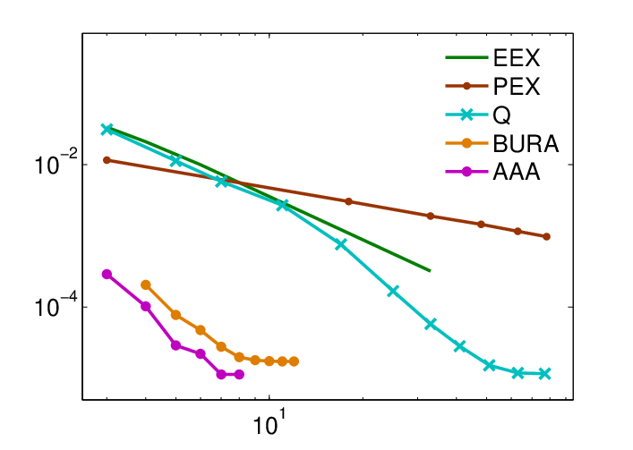
On Figure 7.1 we put together the numerical results of BURA from [38, 40], ${k^{\prime}}$ -Q-method from [14], and the results of three additional methods labeled as: EEX for the elliptic extension method [10] with linear FEM discretization in the auxiliary direction $y$ ; PEX for the pseudo-parabolic extension [71] with Crank-Nicolson discretization in time $t$ ; AAA, based on the Chebfun generated best uniform rational approximation of a discrete set of values of $z^{\alpha}$ on $(\lambda_{1,h},\lambda_{N,h})$ by using the Symbolic Math Toolbox of MATLAB R2008b, [67], introduced and discussed in [43]. The data for these three methods are extracted from Figure 2 of [43]. In agreement with the theory, for any fixed $k$ , BURA outperforms EEX, PEX and ${k^{\prime}}$ -Q methods. We note that rather small $k$ is sufficient to balance the discretization error of order $O(h^{2\alpha})$ (the case if $f\in L^{2}(\Omega)$ ) with BURA error.

As discussed in Section 6.1, the computation of BURA for larger $k$ faces certain problems due to the computational instability of the Remez algorithm. The AAA method avoids this difficulty under the assumption that the extremal eigenvalues of ${\mathbb{A}}$ are available. The so-called “adaptive Antoulas-Anderson” (AAA) [54] algorithm exploits representation of the rational approximant in barycentric form and greedy selection of the support points. The method proposed in [43] is based on AAA approximation of $z^{-\alpha}$ for $z\in[\lambda_{1,h},\lambda_{N,h}]$ , while the BURA method essentially uses the approximation on $[\lambda_{1,h},\infty)$ . According to Remark 6.1, the error of AAA method is always smaller than the error of BURA method. This is also in agreement with the computations of the BURA by Remez algorithm presented in [36]. Figure 7.1 shows that the errors of AAA and BURA have similar behavior with respect to $k$ . When $\lambda_{1,h}$ and $\lambda_{N,h}$ are known, the AAA approximation is cheaper to get for different $\alpha$ and the computations are more stable for larger $k$ . Moreover, if we have bounds $\underline{\lambda}$ and $\overline{\lambda}$ , such that $\underline{\lambda}\leq\lambda_{1,h}$ and $\lambda_{N,h}\leq\overline{\lambda}$ , then the application of AAA method will still generate a good approximation to $z^{-\alpha}$ on $(\underline{\lambda},\overline{\lambda})$ , which gives the AAA method some practical advantage.

7.2. Parallel efficiency

The development of highly efficient parallel algorithms for large-scale problems is a topic of rapidly growing interest. In the case of fractional diffusion problems, the parallel implementation is of even stronger importance.

The following example illustrates how extreme computational demands could appear. Let the problem in $\Omega\subset{\mathbb{R}}^{3}$ be discretized by linear finite elements with a mesh parameter $h$ , and let $f(x)\in L^{2}(\Omega)$ . Then: (i) Standard diffusion: FEM error estimate: $O(h^{2})$ ; $h=10^{-2}$ is needed for $O(10^{-4})$ accuracy, leading to $N=O(10^{6})$ ; (ii) Modest fractional diffusion: FEM error estimate: $O(h^{2\alpha})$ ; for $\alpha=0.5$ , $h=10^{-4}$ is required to get $O(10^{-4})$ accuracy, leading to $N=O(10^{12})$ . The last size is a challenge even for the modern supercomputers.

The first study on parallel solution of fractional diffusion problems was published in [47]. The fractional Laplacian in the unit cube $\Omega=(0,1)^{3}$ is considered, where the seven point stencil is applied to discretize the Laplace operator. The ${k^{\prime}}$ -Q-method with ${k^{\prime}}=1/3$ is used which means 91 auxiliary systems with sparse symmetric and positive definite matrices. The PCG is utilized as a basic iterative solution method for these systems where a parallel multi-grid (MG) implementation from the Trilinos ML package is the preconditioner.

Table 5. Parallel scalability: maximum 61 physical cpu cores per node.

	$N=128^{3}$		$N=256^{3}$
Nodes	T[s]	E[%]	T[s]	E[%]
1	146		989
2	59	124	455	109
4	37	98	244	101

The reported parallel times T[s] and efficiencies E[%] for $\alpha=0.5$ are shown in Table 5. We stress that in this implementation, the distribution of the 91 solves between the nodes is optimized, taking into account the different number of PCG iterations for each of them, needed to reach the stopping criteria of $10^{-10}$ .

Various aspects of the parallel implementation of the surveyed methods are discussed in [22, 23, 52]²² 2 In these papers, the authors have used some of the earlier variants of BURA from [37, 39], which are not robust with respect to the condition number of the matrix ${\mathbb{A}}$ .. A scalability analysis of the PEX, ${k^{\prime}}$ -Q and BURA methods is presented in [23], where the test problem in $\Omega=(0,1)^{3}$ with a CheckerBoard right-hand-side is considered with up to $512^{3}$ unknowns. The EEX method is excluded from the list of studied methods, as less suitable due to the high memory requirements in the 3D case. The discussed question is which parallel algorithm is recommended to achieve a certain accuracy for a given $\alpha\in\{0.25,0.75\}$ .

A less commonly used approach to a comparison analysis of parallel efficiency of EEX, PEX, ${k^{\prime}}$ -Q and BURA methods is proposed in [52]. The presented results are based on using up to 32 nodes of the supercomputer, with a setting of up to 16 cpu cores per node³³ 3 The parallel numerical tests discussed above are performed on the Bulgarian Academy of Sciences supercomputer Avitohol (http://www.iict.bas.bg/avitohol/). . For example, in [52, Table 6.8], the best parallel times to achieve a given accuracy are shown. Similarly, [52, Table 6.9] displays the best speed-ups versus accuracy. The performed analysis has shown that the selection of the best algorithm is problem dependent.

At the end of this section, it is worth to point out that all considered methods have been implemented in their original formulations. Now, after the unified interpretation of all of them (see [43]) as certain rational approximations, the related additive representation as a sum of partial fractions is expected to be used in the development of future parallel algorithms.

8. Challenges beyond the scalar elliptic case

8.1. Time dependent space-fractional diffusion problems

Let us consider the time dependent problem: find $u(x,t)$ for $(x,t)\in\Omega\times(0,T]$ such that

(8.1)

\frac{\partial u(x,t)}{\partial t}+{\mathcal{A}}^{\alpha}u(x,t)=f(x,t)\quad\mbox{and}\quad u(x,0)=v(x),

with $v(x)$ and $T>0$ given initial data, and $T>0$ a real number. In this section, for simplicity of the presentation we will assume that the finite difference method is used to approximate ${\mathcal{A}}$ in space. We introduce also a uniform mesh in time with step size $\tau=T/M$ , $M$ is a given integer parameter. Following the established matrix notations we write the fully explicit two-level scheme in the form:

(8.2)

\frac{{\bf u}^{j+1}-{\bf u}^{j}}{\tau}+{\mathbb{A}}^{\alpha}{\bf u}^{j}=\mathbf{F}^{j},\quad j=1,\ldots,M,

where the upper index $j$ indicates the related mesh function (vector) at the time level $t=j\tau$ . This scheme is conditionally stable.

The following regularized scheme is proposed in [72]

(8.3)

({\mathbb{I}}+\tau{\mathbb{R}})\frac{{\bf u}^{j+1}-{\bf u}^{j}}{\tau}+{\mathbb{A}}^{\alpha}{\bf u}^{j}=\mathbf{F}^{j},\quad j=1,\ldots,M,

${\mathbb{R}}=\sigma(\alpha{\mathbb{A}}+(1-\alpha){\mathbb{I}})$ , proving unconditional stability if $\sigma\geq 0.5$ . To implement the scheme (8.3) one has to perform matrix-vector multiplication with ${\mathbb{A}}^{\alpha}$ . For this purpose the representation ${\mathbb{A}}^{\alpha}={\mathbb{A}}{\mathbb{A}}^{-(1-\alpha)}$ is used and reformulation of the fractional problem to a pseudo-parabolic (see Subsection 4.2) is applied to approximate the solution of systems with ${\mathbb{A}}^{1-\alpha}$ .

The alternative approach proposed in [1] is based on rational approximation of the discrete fractional Laplacian. It is obtained from applying the Gauss-Jacobi quadrature to the integral representation of ${\mathbb{A}}^{\alpha}$ in $[0,1]$ and is described in Subsection 5.2.

The methods form [1, 72] have promising stability properties that are confirmed by numerical tests. The drawback for large scale problems in space is that their accuracy is not robust with respect to the condition number $\kappa({\mathbb{A}})$ . The matrix-vector multiplication with ${\mathbb{A}}^{\alpha}$ could be avoided by applying the unconditionally stable backward Euler scheme

(8.4)

\frac{{\bf u}^{j+1}-{\bf u}^{j}}{\tau}+{\mathbb{A}}^{\alpha}{\bf u}^{j+1}=\mathbf{F}^{j},\quad j=1,\ldots,M.

The implementation of (8.4) requires solution of linear systems with the matrix ${\mathbb{A}}^{\alpha}+\frac{1}{\tau}{\mathbb{I}}$ at each time step $j=1,\ldots,M$ . For this purpose, one can use the BURA method for fractional diffusion reaction problems discussed in Subsection 6.3 with $q=\frac{1}{\tau}$ . The BURA error estimate is robust with respect to $\kappa({\mathbb{A}})$ . In this setting, there appear new challenges related to the numerical stability of the Remez algorithm for $q\gg 1$ . Some combination of BURA and URA methods could be helpful in this context.

8.2. Coupled problems involving fractional diffusion operators

A majority of the real-life applications are described by coupled problems. Among many others, we could mention the fractional diffusion epidemic models, [16], the two-phase flow models based on the Navier-Stokes equations combined with a fractional Allen-Cahn mass-preserving model, [62], or surface quasi-geostrophic flows, [12, 57]. To illustrate some basic ideas and the related challenges we will consider the system of time dependent fractional-in-space diffusion-reaction equations for the unknown functions $u_{\ell}(x,t)$ in the form

(8.5)

\frac{\partial u_{\ell}(x,t)}{\partial t}+{\mathcal{A}}_{\ell}^{\alpha_{\ell}}u(x,t)={\mathcal{R}}_{\ell}(u_{1},\ldots,u_{m})+f_{\ell}(x,t),\quad\ell=1,\ldots,m,

with given initial data $u_{\ell}(x,0)=u_{\ell,0}(x)$ , $\ell=1,\ldots,m$ . The system (8.5) is coupled trough the reaction operators ${\mathcal{R}}_{\ell}(u_{1},\ldots,u_{m})$ . Now, we rewrite the system in the form of abstract Cauchy problem

(8.6)

\frac{\partial U(x,t)}{\partial t}=({\mathcal{A}}^{\alpha}+{\mathcal{R}})U(x,t)+F(x,t),\quad U(x,0)=U_{0}(x),

where ${\mathcal{A}}^{\alpha}:=diag({\mathcal{A}}_{1}^{\alpha_{1}},\dots,{\mathcal{A}}_{m}^{\alpha_{m}})$ and ${\mathcal{R}}$ are the fractional diffusion and the reaction, respectively, $U(x,t)=(u_{1}(x,t),\ldots,u_{m}(x,t))^{T}$ , $F(x,t)=(f_{0}(x,t),\dots,f_{m}(x,t))^{T}$ and $U_{0}(x)=(u_{1,0}(x),\ldots,u_{m,0}(x))^{T}$ .

Nowadays, the operator splitting is a commonly used approach in solving such kind of problems. The basic ideas are associated with the pioneering works of Yanenko, [76], Marchuk, [50] and Strang, [65]. In the case of standard (not fractional) elliptic operator ${\mathcal{A}}$ , i.e. $\alpha_{\ell}\equiv 1$ , the advantages of second (or higher) order splitting methods are well understood. As a principle, they use Crank-Nicolson like approximation of the derivative in time, thus involving in particular matrix-vector multiplication with the discrete diffusion operator. As was discussed in the previous subsection, the development of robust method for multiplication with ${\mathcal{A}}_{h}^{\alpha}$ is still a challenging problem. This is the main reason to restrict our consideration to the following sequential splitting algorithm:

For $(j-1)\tau<t\leq j\tau$ , $j=1,2,\ldots,M$ ,

\begin{array}[]{ll}\quad{\displaystyle\frac{\partial{U_{1}^{j}(x,t)}}{\partial t}}={{\mathcal{A}}^{\alpha}}{U}_{1}^{j}(x,t),\quad{U}_{1}^{j}(x,(j-1)\tau)={U}_{2}^{j-1}(x,(j-1)\tau),&\\ \quad{\displaystyle\frac{\partial{U}_{2}^{j}(x,t)}{\partial t}}={\mathcal{R}}{U}_{2}^{j}(x,t)+F(x,t),\quad{U}_{2}^{j}(x,(j-1)\tau)={U}_{1}^{j}(x,j\tau),&\end{array}

where $\tau=T/M$ is the time step and $U_{2}(x,0)=U_{0}(x)$ . The function $U^{j}_{sp}(x,j\tau)=U^{j}_{2}(x,j\tau)$ is a sequential splitting approximate solution of (8.6).

Here we follow the abstract convergence analysis from [31], assuming that the operators ${\mathcal{A}}$ and $\mathcal{R}$ are bounded with respect to $t\in[0,T]$ and the abstract Cauchy problem (8.6) is well posed. Then, the above sequential splitting is unconditionally stable and the splitting error is $O(\tau)$ [31, Theorem 1]. We will assume also that the backward Euler time-stepping scheme for the fractional diffusion sub-problems is combined with a properly chosen Runge-Kutta solution methods of the sub-problems associated with the reaction operator ${\mathcal{R}}$ , thus ensuring the targeted accuracy of $O(\tau)$ .

There are several different errors in the composite algorithm. Their balancing is of a key importance. Now, for simplicity of the presentation, we will assume that $\alpha_{\ell}=\alpha$ , and that a uniform mesh with mesh parameter $h$ is used for approximation of the diffusion operator. Under certain usual assumptions, the convergence rate of discretization in space of the fractional diffusion problems is $O(h^{2\alpha})$ , see, e.g. [13]. The application of BURA method in the case of backward Euler time-stepping was discussed in the previous subsection, see the paragraph after (8.4). From the numerical data presented in [36] we can deduct that for $q\gg 1$ the BURA error behaves like $O(\frac{1}{q})$ . This follows from the estimate

(8.7)

E_{q,\alpha,k}=C(k,\alpha)E_{\alpha,k}/(q+1)=O\left(e^{-2\pi\sqrt{k\alpha}}/q\right),

which is concluded form (6.18) and the analysis there after (see also, (6.7) and recall that $E_{\alpha,k}=E_{0,\alpha,k}$ ), ((6.8)) and Table 3). Thus, taking $\tau=1/q$ in (8.7) and combining with (6.17), we get the following asymptotic estimate holds true for the BURA error of the fractional diffusion sub-problem with backward Euler discretization in time $O\left(\tau e^{-2\pi\sqrt{k\alpha}}\right)$ , where $k$ is the degree of the best uniform rational approximation. Thus we get that the considered composite sequential splitting algorithm has a total error decay $O(\tau+h^{2\alpha})$ .

9. Concluding remarks

In this survey we discussed various numerical methods for solving equations (3.1) arising in discretization of fractional by powers of multidimensional elliptic problems.

Though quite different in derivation and error analysis these methods have one common underlying feature: they all produce some rational approximation $r_{k}({\mathcal{A}}_{h})=P_{k}({\mathcal{A}}_{h})/Q_{k}({\mathcal{A}}_{h})$ of ${\mathcal{A}}_{h}^{-\alpha}$ so that instead $u_{h}={\mathcal{A}}_{h}^{-\alpha}f_{h}$ we compute $u_{h,k}=r_{k}({\mathcal{A}}_{h})f_{h}$ . Using spectral argument we see easily that the error $u_{h}-u_{h,k}$ is estimated by the error $\max_{z\in[\lambda_{1,h},\lambda_{N,h}]}|z^{-\alpha}-r_{k}(z)|$ . Thus, one concludes that any “good” approximation of $z^{-\alpha}$ on $[\lambda_{1,h},\lambda_{N,h}]$ will produce a solution of (3.1) as well. This is equivalent to finding an approximation of $z^{\alpha}$ on $[\lambda_{N,h}^{-1},\lambda_{1,h}^{-1}]$ , which upon introducing a scaling of ${\mathcal{A}}_{h}$ by $\lambda_{1,h}^{-1}$ , is reduced to minimization in $[\epsilon,1]$ , with $\epsilon=\lambda_{1,h}/\lambda_{N,h}$ .

Since $\epsilon$ is very small (it diminishes like $\min h^{2}$ ) we essentially need to find a “good” approximation on $(0,1]$ to $z^{\alpha}$ , which has singular derivative at $0$ . Remez algorithm for computing this approximation becomes more numerically unstable and computationally expensive for small $\alpha$ and/or large $k$ . Due to the theoretical results [60, Theorem 3], both the zeros $\{\zeta_{i}\}_{1}^{k}$ and poles $\{d_{i}\}_{1}^{k}$ of the BURA $r_{\alpha,k}(z)$ of $z^{\alpha}$ , $z\in[0,1]$ , cluster at zero, when $k$ increases. More precisely, for every choice of $-\infty\leq a\leq b<0$

\lim_{k\to\infty}\frac{1}{\sqrt{k}}card\{\zeta_{i}\in[a,b]\}=\frac{\sqrt{\alpha}}{\pi}\int_{|b|}^{|a|}\frac{dt}{t\sqrt{1+t}}=\lim_{k\to\infty}\frac{1}{\sqrt{k}}card\{d_{i}\in[a,b]\}.

In other words, the number of poles (as well as zeros) on any given interval $(a,b)$ , $a<b<0$ , grows like $\sqrt{k}$ and since the total number is $k$ , this proves that for large $k$ an $O(\sqrt{k})$ of the poles (as well as the zeros) of $r_{\alpha,k}(z)$ are as close to the origin as one wishes. Similar result, [60, Theorem 4] is valid for the extreme points $\{\eta_{i}\}_{1}^{k}$ of the error $r_{\alpha,k}(z)-z^{\alpha}$ . To illustrate the clustering, we give below the distribution of the poles $d_{j}$ , $j=1,\dots,k$ , of $r_{\alpha,k}(t)$ for $k=8$ (see, [36, Table 38]):
$\alpha=0.25$ : $d_{1}=-$ 2.39 e-11, $d_{2}=-$ 8.37 e-9, $d_{3}=-$ 5.95 e-7, $\dots,d_{8}=-$ 1.53;
$\alpha=0.50$ : $d_{1}=-$ 7.35 e-8, $d_{2}=-$ 3.98 e-6, $d_{3}=-$ 7.62 e-4, $\dots,d_{8}=-5.43$ ;
$\alpha=0.75$ : $d_{1}=-$ 2.38 e-6, $d_{2}=-$ 5.93 e-5, $d_{3}=-$ 6.50 e-4, $\dots,d_{8}=-17.9$ .

The clustering of the poles (the extremal points as well) shows that, high numerical accuracy and computer arithmetic precision is needed for computing $r_{\alpha,k}(z)$ , when $\alpha\ll 1$ and/or $k\gg 1$ . This is the most serious challenge for Remez algorithm which exhibits instability while computing $r_{\alpha,k}(z)$ for $k\geq 10$ .

In Section 7.1 we discussed the AAA algorithm. It has been used to generate a best uniform rational approximation of a discrete set of values of $z^{\alpha}$ , $z\in[\lambda_{1,h},\lambda_{N,h}]$ . The Chebfun implementation of AAA algorithm has been successfully used by Hofreither [43] for numerical solution of fractional diffusion problems. The reported numerical results (see, e.g., Fig. 7.1) show that this could be an attractive practical approach allowing to utilize the theoretical advantages of the BURA methods for wide class of applications. But due to the clustering of the poles near zero even this method suffers of instabilities for large $k$ . Based on this observation, Hofreithger in [44] presented a method for computing $r_{\alpha,k}(z)$ using radial basis functions and adaptation procedure. This resulted in an algorithm that is robust with respect to $\alpha$ and $k$ and is the best available method for fining approximately BURA in our opinion.

Moreover, any of the methods discussed in this paper could be rated for accuracy and performance by checking whether they produce a rational approximation with clustering of the poles near the origin. For example, the method of Vabishchevich for solving a pseudo-parabolic equation with constant time stepping (described in Subsection 4.2) will be much less efficient than BURA method. An improvement that uses adaptive time-stepping and produces certain clustering of the poles of the corresponding rational function is presented and justified in [29].

Finally, we conclude with some challenges. As noted in [69], the AAA rational approximation is near-best. By definition, it depends on the spectrum of the system’s matrix. In this sense, the method is not fully robust with respect to the condition number. For example, some further improvements are required to stabilize the convergence, when applied to fractional diffusion reaction problem (6.15) for reaction coefficients $q\gg 1$ , a case beyond the theoretical studies of Stahl [64]. The quality of the AAA approximation depends also from the data (the set of values of the related function) that are approximated. In [43], the values of $z^{\alpha}$ are taken on a uniform mesh of $[\lambda_{1,h},\lambda_{N,h}]$ , in general, not the best choice. One should expect some improvement if the exponential node clustering around the singularity point(s) is taken into account, see e.g., [69]. The last, but not least comment concerns the Chebfun implementation. Although the computational stability of AAA algorithm is ensured, the opportunity to use double (and even higher) precision could be very useful in some more complicated (ill conditioned) problems.

Further progress in computational stability has been recently reported in [44]. The proposed BRASI algorithm is based on the assumption that the best rational approximation of $f(z)$ must interpolate the function at a certain number of interpolation nodes $z_{j}$ . It iteratively rescales the intervals $(z_{j-1},z_{j})$ with the goal of equilibrating the local errors. The barycentric rational formula is used in the implementation. For example, results for $k=93$ , $\alpha=0.25$ and $q=400$ are reported to illustrate the improved stability for $q\gg 1$ .

Acknowledgments

The partial support through the Grant No BG05M2OP001-1.001-0003, financed by the Science and Education for Smart Growth Operational Program (2014-2020) and co-financed by the EU through the European Structural and Investment Funds, and through the Bulgarian NSF Grant No DFNI-DN12/1 is highly appreciated. The work of R. Lazarov has been partially supported by NSF-DMS #1620318 grant.

References

[1] L. Aceto, P. Novati, Rational approximation to the fractional Laplacian operator in reaction-diffusion problems. SIAM J. Sci. Comput. 39, No 1 (2017), A214–A228, DOI: https://doi.org/10.1137/16M1064714.
[2] L. Aceto, P. Novati, Efficient implementation of rational approximations to fractional differential operators. Journal of Scientific Computing 76, No 1 (2018), 651–671, DOI: https://doi.org/10.1007/s10915-017-0633-2.
[3] L. Aceto, P. Novati, Rational approximations to fractional powers of self-adjoint positive operators. Numerische Mathematik 143 (2019), 1–16, DOI: https://doi.org/10.1007/s00211-019-01048-4.
[4] L. Aceto, P. Novati, Fast and accurate approximations to fractional powers of operators. arXiv:2004.09793 (2020).
[5] G. Acosta, J.P. Borthagaray, A fractional Laplace equation: regularity of solutions and finite element approximations. SIAM J. Numer. Anal. 55, No 2 (2017), 472–495, DOI: https://doi.org/10.1137/15M1033952.
[6] G. Acosta, F.M. Bersetche, J.P. Borthagaray, Finite element approximations for fractional evolution problems. Fract. Calc. Appl. Anal. 22, No 3 (2019), 767–794; DOI: 10.1515/fca-2019-0042.
[7] M. Ainsworth, Z. Mao, Fractional phase-field crystal modelling: analysis, approximation and pattern formation. IMA J. of Applied Mathematics 85, No 2 (2020), 231–262, DOI: 10.1093/imamat/hxaa004.
[8] A. Balakrishnan, Fractional powers of closed operators and the semigroups generated by them. Pacific J. Math. 10, No 2 (1960), 419–437.
[9] T. Bærland, M. Kuchta, K.-A. Mardal, Multigrid methods for discrete fractional Sobolev spaces. SIAM J. Sci. Comput. 41, No 2 (2019), A948–A972, DOI: https://doi.org/10.1137/18M1191488.
[10] A. Bonito, J.P. Borthagaray, R.H. Nochetto, E. Otárola, A.J. Salgado, Numerical methods for fractional diffusion. Comput. Visual Sci., 19 (2019), 19–46, DOI: https://doi.org/10.1007/s00791-018-0289-y.
[11] A. Bonito, W. Lei, J.E. Pasciak, Numerical approximation of the integral fractional Laplacian. Numer. Math. 142, No 2 (2019), 235–278, DOI: https://doi.org/10.1007/s00211-019-01025-x.
[12] A. Bonito, M. Nazarov, Numerical simulations of surface-quasi geostrophic flows on periodic domains. Preprint arXiv:2006.01180 (2020).
[13] A. Bonito, W. Lei, J.E. Pasciak, On sinc quadrature approximations of fractional powers of regularly accretive operators. J. of Numerical Mathematics 27, No 2 (2019), 57–68, DOI: 10.1515/jnma-2017-0116.
[14] A. Bonito, J.E. Pasciak, Numerical approximation of fractional powers of elliptic operators. Mathematics of Computation 84, No 295 (2015), 2083–2110, DOI: https://doi.org/10.1090/S0025-5718-2015-02937-8.
[15] A. Bonito, J.E. Pasciak, Numerical approximation of fractional powers of regularly accretive operators. IMA J. Numerical Analysis 37, No 3 (2017), 1245–1273, DOI: https://doi.org/10.1093/imanum/drw042.
[16] D. Brockmann, V. David, A.M. Gallardo, Human mobility and spatial disease dynamics. Reviews of Nonlinear Dynamics and Complexity 2 (2009), 1–24.
[17] L. Caffarelli, L. Silvestre, An extension problem related to the fractional Laplacian. Commun. in Partial Differential Equations 32, No 8 (2007), 1245–1260, DOI: https://doi.org/10.1080/03605300600987306.
[18] L.A. Caffarelli and P.R. Stinga, Fractional elliptic equations, Caccioppoli estimates and regularity. Annales de l’Inst. Henri Poincare (C) Non Linear Analysis, 33, No 3 (2016), 767–807, DOI: https://doi.org/10.1016/j.anihpc.2015.01.004.
[19] A.L. Chang, H.G. Sun, Time-space fractional derivative models for CO2 transport in heterogeneous media. Fract. Calc. Appl. Anal. 21, No 1 (2018), 151–173; DOI: 10.1515/fca-2018-0010.
[20] L. Chen, R. Nochetto, O. Enrique, A.J. Salgado, Multilevel methods for non-uniformly elliptic operators and fractional diffusion. Math. of Computation 85 (2016), 2583–2607, DOI: https://doi.org/10.1090/mcom/3089.
[21] P.G. Ciarlet, The Finite Element Method for Elliptic Problems. Classics in Applied Mathematics, SIAM (2002).
[22] R. Čiegis, V. Starikovičius, S. Margenov, R. Kriauziené, A comparison of accuracy and efficiency of parallel solvers for fractional power diffusion problems. In: Parallel Processing and Applied Mathematics. PPAM 2017. Lecture Notes in Computer Science (Eds: R. Wyrzykowski, J. Dongarra, E. Deelman, K. Karczewski) 10777 (2018), 79–89.
[23] R. Čiegis, V. Starikovičius, S. Margenov, R. Kriauziené, Scalability analysis of different parallel solvers for 3D fractional power diffusion problems. Concurrency and Computation: Practice and Experience, 31, No 19 (2019), DOI: 10.1002/cpe.5163.
[24] R. Čiegis, P.N. Vabishchevich, Two-level schemes of Cauchy problem method for solving fractional powers of elliptic operators. Computers $\&$ Mathematics with Appl. 80, No 2 (2019), 305–315; DOI: 10.1016/j.camwa.2019.08.012.
[25] R. Čiegis, P.N. Vabishchevich, High order numerical schemes for solving fractional powers of elliptic operators. J. of Computational and Appl. Math. 372 (2020); DOI: 10.1016/j.cam.2019.112627.
[26] M. M. Djrbashian, Harmonic Analysis and Boundary Value Problems in the Complex Domain. Birkhäuser Verlag, Basel (1993).
[27] T.A. Driscoll, N. Hale, L. Trefethen, Chebfun Guide. Pafnuty Publications (2014).
[28] V. Druskin, L. Knizhnerman, Extended Krylov subspaces: approximation of the matrix square root and related functions. SIAM J. Matrix Anal. Appl., 19, No 3 (1998), 755–771, DOI: https://doi.org/10.1137/S0895479895292400.
[29] B. Duan, R.D. Lazarov, J.E. Pasciak, Numerical approximation of fractional powers of elliptic operators. IMA J. Numerical Analysis 40, No 3 (2019), 1746–1771; DOI: 10.1093/imanum/drz013.
[30] M. D’Elia, Q. Du, C. Glusa, M. Gunzburger, X. Tian, and Z. Zhou, Numerical methods for nonlocal and fractional models. Preprint arXiv:2002.01401 (2020).
[31] I. Faragó, Splitting methods and their application to the abstract Cauchy problems. In: Numerical Analysis and Its Applications. NAA 2004. Lecture Notes in Computer Science (Eds: Z. Li, L. Vulkov, J. Waśniewski) 3401 (2005), 33–45.
[32] W. H. Gerstle, Introduction to Practical Peridynamics. World Scientific, 2015.
[33] I. Georgieva, S. Harizanov, C. Hofreither, Iterative low-rank approximation solvers for the extension method for fractional diffusion. Computers $\&$ Mathematics with Appl. 80, No 2 (2020), 351–366; DOI: 10.1016/j.camwa.2019.07.016.
[34] G. Gilboa and S. Osher, Nonlocal operators with applications to image processing. Multiscale Modeling & Simulation, 7, No 3 (2008), 1005–1028, DOI: 10.1137/070698592.
[35] G. Grubb, Regularity of spectral fractional Dirichlet and Neumann problems. Mathematische Nachrichten 289, No 7 (2016), 831–844.
[36] S. Harizanov, R. Lazarov, S. Margenov, P. Marinov, The best uniform rational approximation BURA of $t^{\alpha}$ , $t\in[0,1]$ , $\alpha\in(0,1)$ : Applications to solving equations involving fractional powers of elliptic operators. Lecture Notes in Computer Science and Technologies, No 9, IICT-BAS (2019).
[37] S. Harizanov, R. Lazarov, S. Margenov, P. Marinov, Y. Vutov, Optimal solvers for linear systems with fractional powers of sparse SPD matrices. Numerical Linear Algebra with Applications 25, No 4 (2018), 115–128, DOI: 10.1002/nla.2167.
[38] S. Harizanov, R. Lazarov, S. Margenov, P. Marinov, Numerical solution of fractional diffusion–reaction problems based on BURA. Computers $\&$ Mathematics with Appl., 80, No 2, (2020), 316–331; DOI: 10.1016/j.camwa.2019.07.002.
[39] S. Harizanov, R. Lazarov, S. Margenov, P. Marinov, J. Pasciak, Comparison analysis of two numerical methods for fractional diffusion problems based on the best rational approximations of $t^{\gamma}$ on $[0,1]$ . Lecture Notes in Computational Science and Engineering 128 (2019), 165–185.
[40] S. Harizanov, R. Lazarov, S. Margenov, P. Marinov, J. Pasciak. Analysis of numerical methods for spectral fractional elliptic equations based on the best uniform rational approximation. J. of Computational Physics 408 (2020); DOI: 10.1016/j.jcp.2020.109285.
[41] Y. Hatano and N. Hatano, Dispersive transport of ions in column experiments: an explanation of long-tailed profiles. Water Resources Res. 34 (1998), 1027–1033.
[42] N.J. Higham, Functions of Matrices: Theory and Computation. SIAM, 2008.
[43] C. Hofreither, A unified view of some numerical methods for fractional diffusion. Computers & Mathematics with Applications 80, No 2 (2020), 332–350. DOI: 10.1016/j.camwa.2019.07.025.
[44] C. Hofreither, An algorithm for best rational approximation based on barycentric rational interpolation. RICAM-Report No 2020 – 37 (2020).
[45] M. Ilić, I.W. Turner, V. Anh, A numerical solution using an adaptively preconditioned Lanczos method for a class of linear systems related with the fractional Poisson equation. Int. J. Stochastic Analysis 2008 (2009); DOI:10.1155/2008/104525.
[46] T. Kato, Fractional powers of dissipative operators. J. Math. Soc. Japan 13, No 3 (1961), 246–274.
[47] N. Kosturski, S. Margenov, Y. Vutov, Performance Analysis of MG Preconditioning on Intel Xeon Phi: Towards Scalability for Extreme Scale Problems with Fractional Laplacians. In: Large-Scale Sci. Computing. LSSC 2017. Lecture Notes in Computer Sci., Springer, Cham (Eds: I. Lirkov, S. Margenov) 10665 (2018), 304–312.
[48] M. Kwaśnicki, Ten equivalent definitions of the fractional Laplace operator. Fract. Calc. Appl. Anal. 20, No 1, (2017), 7–51; DOI: 10.1515/fca-2017-0002.
[49] A. Lischke, G. Pang, M. Gulian, F. Song, C. Glusa, X. Zheng, Z. Mao, W. Cai, M.M. Meerschaert, M. Ainsworth, G. Karniadakis, What is the fractional Laplacian? A comparative review with new results. J. of Computational Physics 404 (2020); DOI: 10.1016/j.jcp.2019.109009.
[50] G.I. Marchuk, Some applications of splitting-up methods to the solution of problems in mathematical physics. Aplikace Matematiky 1 (1968), 103–132.
[51] P.G. Marinov, A.S. Andreev, A modified Remez algorithm for approximate determination of the rational function of the best approximation in Hausdorff metric. C.R. Acad. Bulg. Sci. 40, No 3 (1987), 13–16.
[52] S. Margenov,T. Rauber, E. Atanassov, F. Almeida, V. Blanco, R. Ciegis, A. Cabrera, N. Frasheri, S. Harizanov, R. Kriauzien, G. Ruenger, P. San Segundo, V. Starikovicius, S. Szabo, B. Zavalnij, Applications for ultra-scale systems. IET Professional Applications of Computing Series 24 (2019), 189–244.
[53] R. Metzler and J. Klafter, The restaurant at the end of the random walk: recent developments in the description of anomalous transport by fractional dynamics. J. Phys. A, 37, No 31 (2004), R161–R208.
[54] Y. Nakatsukasa, O. Séte, L.N. Trefethen, The AAA algorithm for rational approximation, SIAM J. Sci. Comp. 40, No 3 (2018), A1494–A1522, DOI: 10.1137/16M1106122.
[55] R.H. Nochetto, E. Otárola, A.J. Salgado, A PDE approach to fractional diffusion in general domains: a priori error analysis. Found. Comput. Math. 15, No 3 (2015), 733–791.
[56] R.H. Nochetto, E Otárola, A.J. Salgado, A PDE approach to space-time fractional parabolic problems. SIAM J. Numer. Anal. 54, No 2 (2016), 848–873.
[57] J. Pedlosky, Geophysical Fluid Dynamics. Springer Science & Business Media, 2013.
[58] I. Podlubny, Fractional Differential Equations. Acad. Press, San Diego, CA, 1999.
[59] X. Ros-Oton and J. Serra, The Pohozaev identity for the fractional Laplacian. Archive for Rational Mechanics and Analysis 213, No 2, (2014), 587–-628.
[60] E.B. Saff, H. Stahl, Asymptotic Distribution of Poles and Zeros of Best Rational Approximants to $x^{\alpha}$ on $[0,1]$ . Topics in Complex Analysis, Banach Center Publ., Vol. 31, Institute of Mathematics, Polish Academy of Sciences, Warsaw (1995).
[61] A.A. Samarskii, The Theory of Difference Schemes. Ser. Pure and Applied Mathematics, Vol. 240, Marcel Dekker, Inc., New York (2001).
[62] F. Song, C. Xu, G.E. Karniadakis, Computing fractional laplacians on complex-geometry domains: Algorithms and simulations. SIAM J. Sci. Comp., 39, No 4 (2017), A1320–A1344.
[63] H. Stahl, Best uniform rational approximation of $x^{\alpha}$ on $[0,1]$ . Bull. Amer. Math. Soc. (N.S.) 28, No 1 (1993), 116–122.
[64] H.R. Stahl, Best uniform rational approximation of $x^{\alpha}$ on $[0,1]$ . Acta Math. 190, No 2 (2003), 241–306.
[65] G. Strang, On the construction and comparison of difference schemes. SIAM J. Num. Anal. 5 (1968), 506-517.
[66] H.G. Sun, Y. Zhang, D. Baleanu, W. Chen, Y.Q. Chen, A new collection of real world applications of fractional calculus in science and engineering. Commun. Nonlin. Sci. Numer. Simul. 64 (2018), 213–231.
[67] The MathWorks, Numerics::fMatrix–functional calculus for numerical square matrices; http://www.mathworks.com/access/helpdesk/help/toolbox/mupad/numeric/fMatrix.html, (2009).
[68] V. Thomée, Galerkin Finite Element Methods for Parabolic Problems. Springer Ser. in Comput. Mathematics, Vol. 25, Springer-Verlag, Berlin, 2nd Ed. (2006).
[69] L.N. Trefethen, Y. Nakatsukasa, J.A.C. Weideman, Exponential node clustering at singularities for rational approximation, quadrature, and PDEs. arXiv:2007.11828v1 (2020).
[70] P.N. Vabishchevich, Numerical solving the boundary value problem for fractional powers of elliptic operators. CoRR, abs/1402.1636 (2014).
[71] P.N. Vabishchevich, Numerically solving an equation for fractional powers of elliptic operators. J. of Comput. Phys. 282 (2015), 289–302.
[72] P.N. Vabishchevich, Numerical solution of non-stationary problems for a space-fractional diffusion equation. Fract. Calc. Appl. Anal. 19, No 1 (2016), 116–139; DOI: 10.1515/fca-2016-0007.
[73] P.N. Vabishchevich, Numerical solution of time-dependent problems with fractional power elliptic operator. Comput. Methods in Appl. Math. 18, No 1 (2018), 111–128.
[74] P.N. Vabishchevich, Approximation of a fractional power of an elliptic operator. Numer. Lin. Algebra with Appl. 27, No 3 (2020); DOI: 10.1002/nla.2287.
[75] R.S. Varga, A.J. Carpenter, Some numerical results on best uniform rational approximation of $x^{\alpha}$ on [0, 1]. Numerical Algorithms 2, No 2 (1992), 171–185.
[76] N.N. Yanenko, On convergence of the splitting method for heat equation with variable coefficients. J. Comput. Math. Math. Phys. 2, No 5 (1962), 933–937 (in Russian).
[77] J. Xu, L. Zikatanov, The method of alternating projections and the method of subspace corrections in Hilbert space. J. Amer. Math. Soc. 15, No 3 (2002), 573–597, DOI: https://doi.org/10.1090/S0894-0347-02-00398-3.