Kernel regression in high dimensions: Refined analysis beyond double descent
Abstract
In this paper, we provide a precise characterization of generalization properties of high dimensional kernel ridge regression across the under- and over-parameterized regimes, depending on whether the number of training data exceeds the feature dimension . By establishing a bias-variance decomposition of the expected excess risk, we show that, while the bias is (almost) independent of and monotonically decreases with , the variance depends on and can be unimodal or monotonically decreasing under different regularization schemes. Our refined analysis goes beyond the double descent theory by showing that, depending on the data eigen-profile and the level of regularization, the kernel regression risk curve can be a double-descent-like, bell-shaped, or monotonic function of . Experiments on synthetic and real data are conducted to support our theoretical findings.
1 Introduction
Interpolation learning [MM19, HMRT19, BLLT20] has recently attracted growing attention in the machine learning community. This is mainly because current state-of-the-art neural networks appear to be models of this type: they are able to interpolate the training data while still generalize well on test data, even in the presence of label noise [ZBH+16]. It has been empirically observed that other models including random features, decision trees, and as simple as linear regression also exhibit similar phenomenon [BLLT20, BHMM19, LHCS20]. This is somewhat striking as it goes against the conventional wisdom of bias-variance trade-off[CS02]: predictors that generalize well must trade off the model complexity against training data fitting. The double descent theory [BHMM19] resolves this paradox by revisiting the bias-variance trade-off and showing that the model generalization error exhibits a phase transition at the interpolation point: moving away from this point on either side tends to reduce the generalization error.
The double descent phenomenon has recently inspired intense theoretical research [MM19, GLK+20, WX20, LCM20] and has been further extended to multiple descent [CMBK20, LRZ19, AP20] on various models. One line of work formalized the argument that, even when no explicit regularization is imposed, implicit regularization is encoded in the model via the choice of optimization algorithms and techniques, e.g., stochastic gradient descent (SGD) [HRS16], dropout [SHK+14], early stopping [AKT19], and ensemble methods [LJB20]. Different from these “external” schemes, the kernel interpolation estimator [LR20, BRT19] directly benefits from its intrinsic kernel structure that serves as an implicit regularization to help both interpolate and approximate. In fact, (strictly) positive-definite kernels can interpolate an arbitrary number of data points [Wen04], and thus kernel spaces contain (nearly) optimal interpolants [GMMM19, Li20]. Although the kernel space is rich enough to contain models that generalize well, the generalization property of kernel method, for example how it depends on the choice of kernel, its interplay with the data and the level of regularization, still remains unclear. In particular, the question whether the double descent phenomenon exists in the kernel regression models is still unanswered [LR20, BCP20]. As such, refined analyses are needed to have a thorough understanding of kernel estimators, notably in the high dimensional regime of interest. This is indeed the objective of the article.
| eigenvalue decay | (KRR) | |||||
| harmonic decay | ||||||
| 1 | ||||||
| polynomial decay | ||||||
| exponential decay | ||||||
- 1
Here is some constant such that always holds as is required to be large in theory and practice.


Here, we consider the kernel ridge regression (KRR) estimator [CS02, SVGDB+02, LSH+21] in a high dimensional setting with data dimension and size both large, and treat the kernel interpolation as a special case of KRR by taking the explicit regularization to be zero. More precisely, by virtue of the linearization of kernel matrices in high dimensions [LR20, EK10, EKZ+20, LC18, LC19], we disentangle the implicit regularization of kernel interpolation estimators in an explicit manner. As a result, both implicit and explicit regularization schemes can be systematically studied within the proposed framework. Mathematically, KRR aims to solve the following empirical risk minimization problem on a training set with data and responses :
| (1.1) |
where an explicit Tikhonov regularization term induced by a reproducing kernel Hilbert space (RKHS) is added to the least-squares objective. In statistical learning theory [CZ07], the regularization parameter is generally taken to depend on the sample size in such a way that . Here we assume that with some and to cover the interpolation case.
In this paper, we propose a novel bias-variance decomposition of the KRR expected excess risk, and derive non-asymptotic bounds for both bias and variance. This precise assessment leads to fruitful discussions as a function of different data eigenvalue decays and regularization schemes. Our main findings include:
- •
We demonstrate that, for data dimension large, the kernel matrix admits the same eigenvalue decay as , where is the data matrix. So in high dimensions, the eigenvalue decay of is almost determined by the data, as reflected in our error bound for the bias.
- •
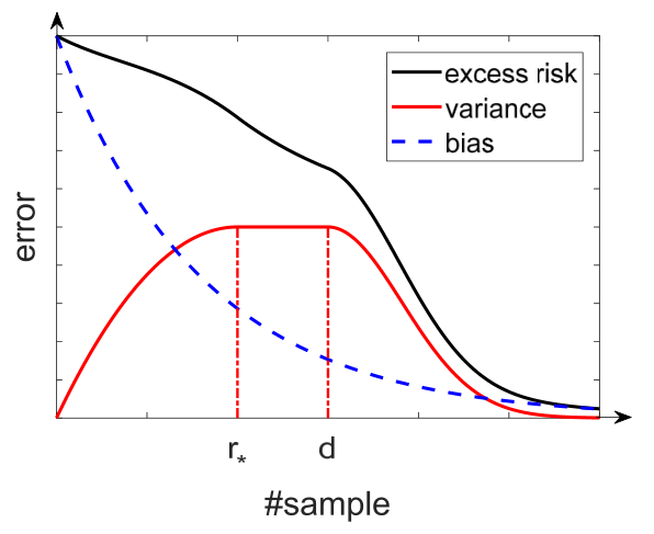
The explicit regularization largely affects the peak point of the variance: a large decreases the model complexity, and thus corresponds to a small value of interpolation point . Table 1 shows that, under a small (or zero) regularization so that with : the error bound for variance monotonically increases with until , as in the red curve of Figure 1(a). Under a moderate regularization with : first increases with until and then decreases. In this case, the peak point will move to the left due to , see the blue curve in Figure 1(a). Under a large regularization with for some constant , monotonically decreases with , as in the green curve of Figure 1(a).
- •
Our error bounds for the bias and the variance exhibit different characteristics. More specifically, the bias bound is (almost) independent of the data/feature dimension and monotonically decreases with at a certain (learning) rate as in the classical learning theory [CZ07, WZ11, SS07]. Besides, the variance bound depends on and , and exhibits monotonic decreasing or unimodal with under different regularizations. Hence, the expected excess risk, as the sum of bias and variance, can be double descent (Figure 1(b)), bell-shaped (Figure 1(c)), or monotonic decreasing (Figure 1(d)), depending on the level of implicit and explicit regularizations. This is in agreement with empirical findings in neural networks [YYY+20].
- •
Our non-asymptotic results show that, for large but fixed , both the variance and bias tends to zero as under , implying that the excess risk approaches zero. Based on this, in the double descent case particularly, the minimum of the expected error in the over-parameterized regime is lower than that in the regime. This claim cannot be obtained from [LR20].
The rest of the paper is organized as follows. We briefly introduce problem settings in Section 2. In Section 3, we present our main results on the generalization property of KRR in high dimensions and briefly sketch the main ideas of the proof. Discussions on the derived error bounds are given in Section 4. In Section 5, we report numerical experiments to support our theoretical results and the conclusion is drawn in Section 6.
2 Problem Settings and Preliminaries
We work in the high dimensional regime for some large with for some constants . For notational simplicity, we denote by : there exists a constant independent of such that , and analogously for and .
2.1 Kernel Ridge Regression Estimator
Let be a metric space and , the instances in the training set are assumed to be independently drawn from a non-degenerate Borel probability measure on . The target function of is defined by
| (2.1) |
where is the conditional distribution of at . Define the response vector and the kernel matrix induced by a positive definite kernel , KRR aims to find a hypothesis such that is a good approximation of the response corresponding to a new instance . This is actually an empirical risk minimization in problem (1.1). By denoting , the closed-form of KRR estimator in Eq. (1.1) is
| (2.2) |
We consider two popular positive definite kernel classes of (i) the inner-product kernel of the form and (ii) the radial kernel function . Here is a nonlinear function that is assumed to be (locally) smooth, as in [EK10, LR20]. Examples include commonly used kernels such as linear kernels, polynomial kernels, Sigmoid kernels, exponential kernels, and Gaussian kernels, to name a few.
The expected (quadratic) risk is defined as and the empirical risk functional is defined on the training set , i.e., . To measure the estimation quality of , one natural way is the expected excess risk: . Specifically, in KRR, the expected excess risk admits , which is exactly in the weighted -space with the norm .
2.2 Background on RKHS
Now we characterize the integral operators defined by a kernel. Given a kernel , its integral operator admits
| (2.3) |
Since is compact, positive definite and self-adjoint, by the spectral theorem (see, Theorem A.5.13 in [SA08]), there exists countable pairs of eigenvalues and eigenfunctions of such that , where are orthogonal basis of and with . Accordingly, by Mercer’s theorem, we have , and there exists a constant such that . It holds by . Based on the data matrix and the integral operator , the empirical integral operator is given by , which converges to the data-free limit at an rate [DMDVR09].
3 Main Results
In this section, we state our main result under some basic/technical assumptions, compare it with existing results, and sketch the main ideas of our proof.
3.1 Basic results
To illustrate our analysis, we need the following three standard assumptions.
Assumption 1.
(Existence of ) We assume .
This is a standard assumption in learning theory and assumes that the target function defined in Eq. (2.1) is indeed realizable, see also [RR19, RR17, CZ07, SS07].
This is a broad model for the noise in the output , containing uniformly bounded or sub-Gaussian noise; and is in fact weaker than the standard Bernstein condition, e.g., in [BK10].
Assumption 3.
This is a standard setting in high-dimensional statistics and random matrix theory [EK10, DW18, LR20, HMRT19, EKZ+20] that assumes that the data are drawn from some not-too-heavy-tailed distribution, with possibly (involved) structure between the entries.
| parameters | inner-product kernels | radial kernels |
|---|---|---|
| 1 |
- 1
, where with and .
To aid our proof, we need some extra results. In [EK10], it has been shown that the kernel matrix in high dimensions can be well approximated by in spectral norm, i.e., as
| (3.1) |
with non-negative parameters , , , and the additional matrix given in Table 2, see some typical examples in Appendix A. Here is the implicit regularization parameter in kernel estimator that depends on the nonlinear function in the kernel and the data structure . According to Eq. (3.1), denote the shortcut , we show in high dimensions that, admits the same eigenvalue decay as and (see details in Appendix B). Subsequently, we introduce the following quantity function
| (3.2) |
which is associated with various quantity functions in [AKT19, DW18, LR20, JŞS+20b, NVKM20] and, as we shall see, plays an important role in determining the variance behavior. We will discuss at length based on different data eigenvalue decays in Section 4.
Formally, our main results of KRR in a high-dimensional regime are stated as follows.
Theorem 1.
Remark: The first term in Eq. (3.3) is the bound of the bias, which is independent of and monotonically decreases with . The sum is the bound of the variance that depends on both and . Note that monotonically decreases with , and approaches to zero for a large . Therefore, the error bound for is the key part of estimates for the variance and will be discussed in in Section 4, where corresponds to the explicit regularization and the implicit regularization. We will demonstrate that can be monotonically decreasing or unimodal under different regularization schemes. Such monotonic bias and unimodal variance can lead to various behaviors of the excess risk, including monotonically decreasing, double descent, and bell-shaped risk curve, as illustrated in Figure 1 of introduction.
3.2 Refined result
Based on the basic result, if we consider two additional assumptions, i.e., extending Assumption 1 by considering the regularity of and studying spectral decay of via complexity of , we can obtain a refined result.
Assumption 4.
(Source condition [CZ07]) For some , there exists satisfying such that .
It has been widely used in the literature of learning theory to assess the regularity of [CZ07, ZDW13, RR17], which indicates belongs to the range space of . Assumption 1 is the worst case of Assumption 4 by choosing since .
Assumption 5.
(Capacity condition [CZ07]) For any , there exist and such that
The notation denotes the “effective dimension” and can be regarded as a “measure of size” of the RKHS. This is a natural and widely used assumption in the literature [CZ07, ZDW13, RR17]. Assumption 5 always holds for and where as is a trace class operator. Its kernel matrix form is [AKM+17, LTOS19]. While Assumption 5 can be further refined to obtain a bound that depends on [PRDVR20], here we focus on the eigenvalue decay of , see Section 4 for details.
Based on the above discussion, we obtain a refined result of Theorem 1 as below.
Theorem 2.
Remark: Compared to classical learning theory results [FS17] achieving learning rates, the parameter in our results only effects the selection range of , which is nearly independent of the learning rates to some extent. That means, the spectral decay of a kernel function in high dimensions is almost irrelevant to its kernel type. In fact, the eigenvalue decay of the kernel matrix in our model largely depends on the data, which is in essence different from classical learning theory results. Therefore, our result reflects a certain “universality” on the kernel function in high dimensional problems, which shows consistency to [EK10].
3.3 Related work
We provide non-asymptotic results that systematically analyze both implicit and explicit regularization schemes within a unified framework.
Implicit regularization in kernel/linear interpolation: Implicit regularization can be induced by minimum norm solutions in linear interpolation [DLM19, KLS20], or the curvature of the kernel function in kernel interpolation [LR20]. Compared to the risk curve in [LR20] that converges to a non-zero constant, the risk curve in our results tends to zero when . Hence our result demonstrates that, in the double descent case, the minimum of the expected risk in the second descent is lower than the first descent; while the same claim cannot be obtained from [LR20]. Besides, under the basic case, our bias bound is based on the eigen-decay (trends) of the kernel matrix and thus can be (almost) independent of , achieving an optimal learning rate in a minimax case. This is different from [LR20] that corresponds to the sum of tailed eigenvalues of . Specifically, if we directly set to zero, our result for the bias still holds, which can be bounded by .
Explicit regularization in kernel/linear regression: We provide non-asymptotic results that refine a series of asymptotic analyses, e.g., the Stieltjes transform approach in [HMRT19, EKZ+20, YYY+20, JŞS+20a] and the statistical mechanic approach in [CBP20]. In fact, by considering the limiting eigenvalue distribution of via its Stieltjes transform , for the solution to the popular Marc̆enko–Pastur equation [MP67], our error bound recovers [HMRT19, Theorem 5] with and isotropic features . Finite sample analyses are often based on a finer control of the Stieltjes transform [JŞS+20b] or the effective rank [BLLT20, CL20]. However, the aforementioned results are generally limited to Gaussian [JŞS+20b, NVKM20] and sub-Gaussian data [BLLT20, CL20, CC20], or Gaussian covariates [RMR20]. Here we consider a much broader family of distributions. Besides, under some specific situations, the regularization parameter in (generalized) linear regression can be negative [KLS20] or optimal tuned [NVKM20, WX20] so as to generalize well. Recent research [GMMM19, LRZ19, BCP20] on kernel regression in shows different trends.
3.4 Proof framework
The proof of our results is fairly technical and lengthy, and we briefly sketch some main ideas of Theorem 2 here. Note that, Theorem 1 is a special case of Theorem 2 by taking and . The modified error decomposition, the error bounds of variance for radial kernels, and estimates for bias are the main elements of novelty in the proof.
In order to estimate the error in the space, we need the following intermediate functions. Define , where is the identity operator, then is actually the minimizer of the following problem . Besides, by defining
we have . Accordingly, the variance-bias decomposition is stated in the following lemma, with proof deferred to Appendix C.
Lemma 3.1.
Let be the minimizer of problem (1.1), can be bounded by
where the bias is defined as
| (3.5) |
where and the variance is defined as
| (3.6) |
where satisfying .
4 Discussion on Error Bounds
In this section, we discuss our Theorem 2 for different eigenvalue profiles of in the two regimes of and . Since shares the same eigenvalue decay as and (see Proposition B.1 in Appendix B), we do not distinguish the eigen-decay of these two data matrices in the subsequent discussions. We first focus on the variance that can be unimodal or monotonically decreasing with under different regularization schemes. Subsequently, we investigate the total risk curve as the sum of bias and variance. Note that has different numbers of non-zero eigenvalues under the two regimes, we denote , which, as we shall see, plays a significant role in characterizing the different cases of our bounds.
4.1 Variance trend for
We consider here three eigenvalue decays of : harmonic, polynomial, and exponential decay [Bac13, LTOS19].
| eigenvalue decay | ||
|---|---|---|
| harmonic decay | 0 | |
| polynomial decay | with | |
| exponential decay | with | |
Proposition 4.1.
Under the three eigenvalue decays in Table 3, denote , then the quantity function with can be bounded by
1) harmonic decay:
.
2) polynomial decay:
, where is some constant.
3) exponential decay: .
Proof The proof can be found in Appendix F. ∎
Harmonic decay: .
For , i.e., the ridgeless case, we have , and , which indicates increases with in the regime. For , taking , we have . To investigate the monotonicity of , define , we find that, a large leads to a small . According to the relationship between , , and , we can conclude that (see Table 1 and the red curve in Figure 1(a)):
When , will increase with until and then remain unchanged when .
When , there are various trends as follows:
1) if , this is the same as the case;
2) if , will increase with until , and then remain unchanged when ;
3) if , will increase with until and then decrease with until , and stay unchanged on ;
4) If such that always holds for some constant , we have increases with until , and then stays unchanged on .
Remark that, for , we have and thus , so that always decreases with until .
Polynomial decay: .
Similar to above, define , we obtain results similar to the case of harmonic decay, but with different thresholds: and , see Table 1 for details.
Exponential decay: .
Here we consider the monotonicity of the function with to study the trend of regarding to . Let be the solution of the equation , then we have the similar conclusion with that of harmonic decay and polynomial decay by the relationship between , , and , see Table 1 for details. More specifically, under some certain conditions, is able to monotonically decrease with , refer to Appendix F.1 for details.
4.2 Variance trends for and total risk
Different from the above case, the current regime admits that has at most non-zero eigenvalues. In this under-parameterized regime, we are particularly interested in the behavior as . In Appendix F.2, we prove that approaches to zero as under the above three eigenvalue decays.
Based on the above discussions in the and regimes, we conclude that, the variance can be unimodal (small regularization) or decreasing (large regularization) as grows, which, together with the fact that the bias is monotonically decreasing with , leads to the following three configurations for the total risk: (i) if the bias dominates at small and then decays fast (i.e., with a small regularization), we observe a double descent curve as in Figure 1(b); (ii) if the bias dominates but decays slowly (with a large regularization), the risk curve will be monotonic decreasing as in Figure 1(d); (iii) if the variance dominates, a bell-shaped risk curve as in Figure 1(c) will be observed.


5 Numerical Results
In this section, experiments are conducted to validate our theoretical results11 1 The source code of our implementation can be found in http://www.lfhsgre.org.. Polynomial kernel of degree and Gaussian kernel are evaluated on 1) a synthetic dataset that satisfies our technical assumptions and 2) a subset of the YearPredictionMSD dataset [Cha08] with 1,000 data samples and , to study our derived error bounds for the bias and variance. More experimental results can be found in Appendix G.
Eigenvalue decay equivalence: Here we study the eigenvalue decay of the original polynomial/Gaussian kernel matrices and their linearization on the subset of YearPredictionMSD dataset. Note that, polynomial kernels admit independent of (see in Table 4), so we use the linearization for this kernel. Results in Figure 2 demonstrate that, the original nonlinear kernels admit the same eigenvalue decay as . More experimental results on various dataset can be found in Appendix G.1.
Risk curves on synthetic dataset: To quantitatively assess our derived error bounds for the bias and variance, we generate a synthetic dataset under a known , with harmonic decay for the data as an illustrating example. More experimental results on different eigenvalue decays refer to Appendix G.2. To be specific, we assume with target function and Gaussian noise having zero-mean and unit-variance. The feature dimension is set to 500. The samples are generated from (and thus with ) by the following steps: (i) take as a diagonal matrix with its diagonal entries following with harmonic decay, i.e., . (ii) take as a random orthogonal matrix22 2 We generate a random Gaussian matrix and use the QR decomposition to obtain an orthogonal matrix [YSC+16]. such that also has a harmonic eigen-decay with having almost i.i.d entries.
Accordingly, the above generation process satisfies Assumption 3, and also admits the same eigenvalue decay as , which can be used to validate our discussion in Section 4. In this setting, the expected excess risk, the bias, and the variance can be directly computed to validate our derived error bounds. The experimental results are validated across 10 trials. Specifically, to disentangle the implicit regularization effect of KRR on the final result, we apply the linearization of the polynomial/Gaussian kernel by setting in Eq. (3.1). In this case, the explicit is the only regularization in KRR. In our model, is empirically set to to avoid a large when is small.
Figures 3 and 4 show results under the harmonic decay setting for the linearization of the polynomial/Gaussian kernel, respectively. We observe that: 1) our error bound exhibits the same trend as the true variance; 2) in this case, the variance dominates and we thus obtain a bell-shaped risk curve that first increases and then decreases; 3) as decreases, increases and the peak point of the variance occurs at smaller and smaller ; 4) the bias monotonically decreases with , which corresponds to our error bound for the bias at a certain rate in Theorem 2 by taking as the used is smooth enough to achieve a good approximation error; 5) in our high-dimensional regimes, different kernels lead to the same convergence rates of the bias, which verifies our results but is different from those in classical learning theory.


Risk curves on the real-world datasets: Figure 5(a) shows the relative mean squared error (RMSE) of kernel ridgeless regression and its linearization in Eq. (3.1) on a subset (1,000 examples) of the YearPredictionMSD dataset averaged on 10 trials. Figure 5(b) shows the classification accuracy of such two methods on the MNIST dataset [LBBH98]. To evaluate the effectiveness of our error bounds, we plot the re-scaled with . It can be found that, kernel interpolation estimator generalizes well due to the implicit regularization, i.e., , which also exhibits a bell-shaped risk curve as our theoretical results suggest. However, in Figure 5(b), the risk curve monotonically decreases with on the MNIST dataset [LBBH98], and at the same time kernel interpolation estimator and its linearization appear to generalize well. This observation may due to the implicit regularization parameter in Eq. (3.1) (of order on this dataset) that plays a fundamental role of “self-regularization”. Accordingly, the proposed analysis provides access to the high-dimensional classification problem that may establish more involved behavior than double descent, despite a clear mismatch between real-world data and the technical Assumption 3, thereby conveying a strong practical motivation for the present analysis.
6 Conclusion
We derived non-asymptotic expressions for the expected excess risk of kernel ridge regression estimators in the under- and over-determined regimes. The used linearization technique of nonlinear smooth kernel allows us to discuss the impact of implicit and explicit regularization in a systematic manner. Our refined analysis demonstrates that the monotonic bias and unimodal variance are able to exhibit various trends of risk curves. Since it is enough to require that the kernel function is differentiable in a neighborhood, our results further extend to the case of Laplace kernels [RZ19].
Acknowledgements
The research leading to these results has received funding from the European Research Council under the European Union’s Horizon 2020 research and innovation program / ERC Advanced Grant E-DUALITY (787960). This paper reflects only the authors’ views and the Union is not liable for any use that may be made of the contained information. This work was supported in part by Research Council KU Leuven: Optimization frameworks for deep kernel machines C14/18/068; Flemish Government: FWO projects: GOA4917N (Deep Restricted Kernel Machines: Methods and Foundations), PhD/Postdoc grant. This research received funding from the Flemish Government (AI Research Program). This work was supported in part by Ford KU Leuven Research Alliance Project KUL0076 (Stability analysis and performance improvement of deep reinforcement learning algorithms), EU H2020 ICT-48 Network TAILOR (Foundations of Trustworthy AI - Integrating Reasoning, Learning and Optimization), Leuven.AI Institute.
References
- [AKM+17] Haim Avron, Michael Kapralov, Cameron Musco, Christopher Musco, Ameya Velingker, and Amir Zandieh, Random Fourier features for kernel ridge regression: Approximation bounds and statistical guarantees, the 34th International Conference on Machine Learning, 2017, pp. 253–262.
- [AKT19] Alnur Ali, J Zico Kolter, and Ryan J Tibshirani, A continuous-time view of early stopping for least squares regression, International Conference on Artificial Intelligence and Statistics, 2019, pp. 1370–1378.
- [AP20] Ben Adlam and Jeffrey Pennington, The neural tangent kernel in high dimensions: Triple descent and a multi-scale theory of generalization, International Conference on Machine Learning, PMLR, 2020, pp. 74–84.
- [Bac13] Francis Bach, Sharp analysis of low-rank kernel matrix approximations, Conference on Learning Theory, 2013, pp. 185–209.
- [BCP20] Blake Bordelon, Abdulkadir Canatar, and Cengiz Pehlevan, Spectrum dependent learning curves in kernel regression and wide neural networks, International Conference on Machine Learning, 2020, pp. 1–11.
- [BHMM19] Mikhail Belkin, Daniel Hsu, Siyuan Ma, and Soumik Mandal, Reconciling modern machine-learning practice and the classical bias–variance trade-off, the National Academy of Sciences 116 (2019), no. 32, 15849–15854.
- [BK10] Gilles Blanchard and Nicole Krämer, Optimal learning rates for kernel conjugate gradient regression, Advances in Neural Information Processing Systems, 2010, pp. 226–234.
- [BLLT20] Peter L. Bartlett, Philip M. Long, Gábor Lugosi, and Alexander Tsigler, Benign overfitting in linear regression, the National Academy of Sciences (2020).
- [BRT19] Mikhail Belkin, Alexander Rakhlin, and Alexandre B Tsybakov, Does data interpolation contradict statistical optimality?, International Conference on Artificial Intelligence and Statistics, 2019, pp. 1611–1619.
- [CBP20] Abdulkadir Canatar, Blake Bordelon, and Cengiz Pehlevan, Statistical mechanics of generalization in kernel regression, arXiv preprint arXiv:2006.13198 (2020).
- [CC20] Emmanuel Caron and Stephane Chretien, A finite sample analysis of the double descent phenomenon for ridge function estimation, arXiv preprint arXiv:2007.12882 (2020).
- [Cha08] Chih-Chung Chang, LibSVM data: Classification, regression, and multi-label, http://www. csie. ntu. edu. tw/˜cjlin/libsvmtools/datasets/ (2008).
- [CL20] Geoffrey Chinot and Matthieu Lerasle, Benign overfitting in the large deviation regime, arXiv preprint arXiv:2003.05838 (2020).
- [CMBK20] Lin Chen, Yifei Min, Mikhail Belkin, and Amin Karbasi, Multiple descent: Design your own generalization curve, arXiv preprint arXiv:2008.01036 (2020).
- [CS02] Felipe Cucker and Steve Smale, On the mathematical foundations of learning, Bulletin of the American mathematical society 39 (2002), no. 1, 1–49.
- [CZ07] Felipe Cucker and Dingxuan Zhou, Learning theory: an approximation theory viewpoint, vol. 24, Cambridge University Press, 2007.
- [DLM19] Michał Dereziński, Feynman Liang, and Michael W Mahoney, Exact expressions for double descent and implicit regularization via surrogate random design, arXiv preprint arXiv:1912.04533 (2019).
- [DMDVR09] Christine De Mol, Ernesto De Vito, and Lorenzo Rosasco, Elastic-net regularization in learning theory, Journal of Complexity 25 (2009), no. 2, 201–230.
- [DW18] Edgar Dobriban and Stefan Wager, High-dimensional asymptotics of prediction: Ridge regression and classification, Annals of Statistics 46 (2018), no. 1, 247–279.
- [EK10] Noureddine El Karoui, The spectrum of kernel random matrices, Annals of Statistics 38 (2010), no. 1, 1–50.
- [EKZ+20] Khalil Elkhalil, Abla Kammoun, Xiangliang Zhang, Mohamed-Slim Alouini, and Tareq Al-Naffouri, Risk convergence of centered kernel ridge regression with large dimensional data, IEEE Transactions on Signal Processing 68 (2020), 1574–1588.
- [FS17] Simon Fischer and Ingo Steinwart, Sobolev norm learning rates for regularized least-squares algorithm, arXiv preprint arXiv:1702.07254 (2017).
- [GLK+20] Federica Gerace, Bruno Loureiro, Florent Krzakala, Marc Mézard, and Lenka Zdeborová, Generalisation error in learning with random features and the hidden manifold model, International Conference on Machine Learning, 2020, pp. 3452–3462.
- [GMMM19] Behrooz Ghorbani, Song Mei, Theodor Misiakiewicz, and Andrea Montanari, Linearized two-layers neural networks in high dimension, Annals of Statistics (2019).
- [GSW17] Zheng-Chu Guo, Lei Shi, and Qiang Wu, Learning theory of distributed regression with bias corrected regularization kernel network, Journal of Machine Learning Research 18 (2017), no. 1, 4237–4261.
- [HMRT19] Trevor Hastie, Andrea Montanari, Saharon Rosset, and Ryan J. Tibshirani, Surprises in high-dimensional ridgeless least squares interpolation, arXiv preprint arXiv:1903.08560 (2019).
- [HRS16] Moritz Hardt, Ben Recht, and Yoram Singer, Train faster, generalize better: Stability of stochastic gradient descent, International Conference on Machine Learning, 2016, pp. 1225–1234.
- [JŞS+20a] Arthur Jacot, Berfin Şimşek, Francesco Spadaro, Clément Hongler, and Franck Gabriel, Implicit regularization of random feature models, International Conference on Machine Learning, 2020, pp. 4631–4640.
- [JŞS+20b] , Kernel alignment risk estimator: Risk prediction from training data, Advances in Neural Information Processing Systems, 2020, pp. 1–9.
- [KLS20] Dmitry Kobak, Jonathan Lomond, and Benoit Sanchez, The optimal ridge penalty for real-world high-dimensional data can be zero or negative due to the implicit ridge regularization, Journal of Machine Learning Research 21 (2020), no. 169, 1–16.
- [LBBH98] Yann Lecun, Leon Bottou, Yoshua Bengio, and Patrick Haffner, Gradient-based learning applied to document recognition, the IEEE 86 (1998), no. 11, 2278–2324.
- [LC18] Zhenyu Liao and Romain Couillet, On the spectrum of random features maps of high dimensional data, the International Conference on Machine Learning, 2018, pp. 3063–3071.
- [LC19] , A large dimensional analysis of least squares support vector machines, IEEE Transactions on Signal Processing 67 (2019), no. 4, 1065–1074.
- [LCM20] Zhenyu Liao, Romain Couillet, and Michael Mahoney, A random matrix analysis of random fourier features: beyond the gaussian kernel, a precise phase transition, and the corresponding double descent, Neural Information Processing Systems, 2020.
- [LD20] Sifan Liu and Edgar Dobriban, Ridge regression: Structure, cross-validation, and sketching, International Conference on Learning Representations, 2020.
- [LGZ17] Shao-Bo Lin, Xin Guo, and Ding-Xuan Zhou, Distributed learning with regularized least squares, Journal of Machine Learning Research 18 (2017), no. 1, 3202–3232.
- [LHCS20] Fanghui Liu, Xiaolin Huang, Yudong Chen, and Johan A.K. Suykens, Random features for kernel approximation: A survey in algorithms, theory, and beyond, arXiv preprint arXiv:2004.11154 (2020).
- [Li20] Weilin Li, Generalization error of minimum weighted norm and kernel interpolation, arXiv preprint arXiv:2008.03365 (2020).
- [LJB20] Daniel LeJeune, Hamid Javadi, and Richard Baraniuk, The implicit regularization of ordinary least squares ensembles, International Conference on Artificial Intelligence and Statistics, 2020, pp. 3525–3535.
- [LR20] Tengyuan Liang and Alexander Rakhlin, Just interpolate: Kernel “ridgeless” regression can generalize, Annals of Statistics 48 (2020), no. 3, 1329–1347.
- [LRZ19] Tengyuan Liang, Alexander Rakhlin, and Xiyu Zhai, On the multiple descent of minimum-norm interpolants and restricted lower isometry of kernels, Annual Conference on Learning Theory, 2019, pp. 1–32.
- [LSH+21] Fanghui Liu, Lei Shi, Xiaolin Huang, Jie Yang, and Johan A.K. Suykens, Analysis of regularized least squares in reproducing kernel kreĭn spaces, Machine Learning (2021), 1–20.
- [LTOS19] Zhu Li, Jean-Francois Ton, Dino Oglic, and Dino Sejdinovic, Towards a unified analysis of random Fourier features, the 36th International Conference on Machine Learning, 2019, pp. 3905–3914.
- [MM19] Song Mei and Andrea Montanari, The generalization error of random features regression: Precise asymptotics and double descent curve, arXiv preprint arXiv:1908.05355 (2019).
- [MP67] Vladimir A Marčenko and Leonid Andreevich Pastur, Distribution of eigenvalues for some sets of random matrices, Mathematics of the USSR-Sbornik 1 (1967), no. 4, 457.
- [NVKM20] Preetum Nakkiran, Prayaag Venkat, Sham Kakade, and Tengyu Ma, Optimal regularization can mitigate double descent, arXiv preprint arXiv:2003.01897 (2020).
- [PRDVR20] Nicolò Pagliana, Alessandro Rudi, Ernesto De Vito, and Lorenzo Rosasco, Interpolation and learning with scale dependent kernels, arXiv preprint arXiv:2006.09984 (2020).
- [RCR13] Alessandro Rudi, Guillermo D Canas, and Lorenzo Rosasco, On the sample complexity of subspace learning, Advances in Neural Information Processing Systems, 2013, pp. 2067–2075.
- [RMR20] Dominic Richards, Jaouad Mourtada, and Lorenzo Rosasco, Asymptotics of ridge (less) regression under general source condition, arXiv preprint arXiv:2006.06386 (2020).
- [RR17] Alessandro Rudi and Lorenzo Rosasco, Generalization properties of learning with random features, Advances in Neural Information Processing Systems, 2017, pp. 3215–3225.
- [RR19] Dominic Richards and Patrick Rebeschini, Optimal statistical rates for decentralised non-parametric regression with linear speed-up, Advances in Neural Information Processing Systems, 2019, pp. 1216–1227.
- [RZ19] Alexander Rakhlin and Xiyu Zhai, Consistency of interpolation with laplace kernels is a high-dimensional phenomenon, Conference on Learning Theory, 2019, pp. 2595–2623.
- [SA08] Ingo Steinwart and Christmann Andreas, Support vector machines, Springer Science and Business Media, 2008.
- [SHK+14] Nitish Srivastava, Geoffrey Hinton, Alex Krizhevsky, Ilya Sutskever, and Ruslan Salakhutdinov, Dropout: a simple way to prevent neural networks from overfitting, Journal of Machine Learning Research 15 (2014), no. 1, 1929–1958.
- [SS07] Ingo Steinwart and Clint Scovel, Fast rates for support vector machines using Gaussian kernels, Annals of Statistics 35 (2007), no. 2, 575–607.
- [SVGDB+02] Johan A.K. Suykens, Tony Van Gestel, Jos De Brabanter, Bart De Moor, and Joos Vandewalle, Least squares support vector machines, World Scientific, 2002.
- [SZ07] Steve Smale and Ding-Xuan Zhou, Learning theory estimates via integral operators and their approximations, Constructive Approximation 26 (2007), no. 2, 153–172.
- [Wen04] Holger Wendland, Scattered data approximation, vol. 17, Cambridge university press, 2004.
- [WX20] Denny Wu and Ji Xu, On the optimal weighted regularization in overparameterized linear regression, Advances in Neural Information Processing Systems, 2020, pp. 1–11.
- [WZ11] Cheng Wang and Ding-Xuan Zhou, Optimal learning rates for least squares regularized regression with unbounded sampling, Journal of Complexity 27 (2011), no. 1, 55–67.
- [YSC+16] Felix Xinnan Yu, Ananda Theertha Suresh, Krzysztof Choromanski, Daniel Holtmannrice, and Sanjiv Kumar, Orthogonal random features, Advances in Neural Information Processing Systems, 2016, pp. 1975–1983.
- [YYY+20] Zitong Yang, Yaodong Yu, Chong You, Jacob Steinhardt, and Yi Ma, Rethinking bias-variance trade-off for generalization of neural networks, the International Conference on Machine Learning, 2020.
- [ZBH+16] Chiyuan Zhang, Samy Bengio, Moritz Hardt, Benjamin Recht, and Oriol Vinyals, Understanding deep learning requires rethinking generalization, arXiv preprint arXiv:1611.03530 (2016).
- [ZDW13] Yuchen Zhang, John Duchi, and Martin Wainwright, Divide and conquer kernel ridge regression, Conference on Learning Theory, 2013, pp. 592–617.
Appendix is organized as follows.
- •
- •
In Section B, we demonstrate that, a kernel matrix in high dimensions admits the same eigenvalue decay as and .
- •
- •
Section F discusses the quantity function based on three eigenvalue decays: harmonic decay, polynomial decay, and exponential decay in the and regimes.
- •
Some additional experiments are presented in Section G to further validate our theoretical results.
Appendix A Examples of kernels and their linearizations
In this section, we present linearization of some typical kernels by Eq. (3.1). Here we assume that to ensure the positive definiteness of the approximated kernel matrix . Table 4 reports the results of three inner-product kernels including polynomial kernel, linear kernel, exponential kernel; as well as a radial kernel: the common-used Gaussian kernel. We can find that . Specifically, avoids a trivial solution.
| kernel | formulation | |||
|---|---|---|---|---|
| polynomial kernels | ||||
| linear kernel | ||||
| exponential kernel | ||||
| Gaussian kernel |
Appendix B Eigenvalue decay equivalence
In this section, we demonstrate that, in high dimensions, a kernel matrix induced by inner-product kernels or radial kernels admits the same eigenvalue decay as and .
For notational simplicity, denote the inner-product kernel matrix and its linearization ; the radial kernel matrix and its linearization .
Proposition B.1.
The inner-product kernel matrix admits the same eigenvalue decay as and .
Proof According to Theorem 2.1 in [EK10], the inner-product kernel matrix can be well approximated by with
in a spectral norm sense, where , , are given in Table 2. As a result, with high probability, the inner-product kernel matrix and its linearization has the same eigenvalue. That means, admits the same eigenvalue decay as via a constant shift .
Next, we shall demonstrate that admits the same eigenvalue decay as . Since is a rank-one matrix with , with Weyl’s inequality and , we have
and
so that the eigenvalue of interlaced with those of . We can thus conclude that the eigenvalue decay of is the same as that of with a constant shift and scaling, which do not effect the trend of eigenvalue decay. Accordingly, the inner-product-type kernel matrix and its linearization , admit the same eigenvalue decay as , which concludes the proof. ∎
Proposition B.1 also provides a justification to study the eigenvalue decay of a radial kernel matrix. According to Theorem 2.2 in [EK10], the radial kernel matrix can be well approximated by with
in a spectral norm sense, where , , are given in Table 2. Recall , where with , we find that is a rank 2 matrix with its eigenvalues , and thus we have .33 3 This can be proved using rank-one decomposition of . Hence, by virtue of Proposition B.1, apart from the top 5 eigenvalues of the radial kernel matrix , its remaining eigenvalues follow with
Accordingly, admits the same eigenvalue decay as .
Appendix C Proof of Lemma 3.1
Proof By virtue of the closed form of the KRR estimator in Eq. (2.2) and , we have
where . According to , we then have
Based on the definition of , we decompose as
which concludes our proof. ∎
Appendix D Proof for the bias
The error bound for the bias is given by the following theorem.
Theorem 3.
In our error decomposition, is independent of data that corresponds to the approximation error in learning theory [CZ07]; while the first term depends on , termed as bias-sample error. To prove Theorem 3, we need to bound the approximation error and the bias-sample error as follows.
D.1 Bound approximation error
In learning theory, the approximation error can be estimated by the source condition in Assumption 4.
D.2 Bound bias-sample error
To bound the bias-sample error , we need the following lemma.
Lemma D.2.
Then the bias-sample error can be decomposed into several parts.
Lemma D.3.
Under Assumption 4, we have
Proof [Proof of Lemma D.3] According to the definition of and , we have
Due to for any bounded positive operator , we have
Further, by virtue of the first order decomposition of operator difference: for any invertible bounded operator and using the source condition in Assumption 4, the above equation can be further expressed as
Besides, using with for any bounded linear operator and positive semi-definite operator in Proposition 9 in [RR17], we have
where we choose , , and . Accordingly, we can conclude our proof due to and . ∎
Remark: The proof framework of Lemma D.3 is similar to Lemma 4 in [RR17] but we consider a more general case than in [RR17]. Although appears to be unattainable as claimed in [RR17], we follow with [LGZ17, GSW17] on a quite general case with .
To prove Theorem 3, we also need the following two lemmas.
Lemma D.4.
(Proposition 6 in [RR17]) Let , it holds with probability at least that
Lemma D.5.
For any , with probability at least , we have
Proof [Proof of Lemma D.5] By virtue of a second order decomposition of operator difference in Lemma 16 [LGZ17], we have
which leads to
| (D.1) |
Accordingly, denote and , we can derive that
where by Lemma D.2. The first inequality holds by with for positive operators and on Hilbert spaces [BK10]. The second inequality can be derived by Eq. (D.1), and . ∎
Remark: Lemma 7.2 in [RCR13] gives by assuming ; whereas our result does not require extra conditions on .
Based on the above lemmas, we are ready to prove Theorem 3.
Proof [Proof of Theorem 3] We first estimate in Lemma D.5 by taking and the capacity condition in Assumption 5: with . Accordingly, we have
where we use due to in the last inequality. Since converges to zero when is large enough, we require to ensure a positive convergence rate, which implies . Then we bound by Lemma D.2. By virtue of for any and , we have
where the second one admits by the capacity condition in Assumption 5. Similarly, to bound by Lemma D.4, we can derive that
Combining the above three inequalities, we have
where is independent of and .
Finally, the bias can be bounded by
where the third inequality holds by due to , and are some constants independent of and . Accordingly, we can conclude the proof. ∎
Appendix E Proof for the variance
Formally, we have the following theorem to bound the variance.
Theorem 4.
For inner-product kernels, our proof framework follows [LR20], and is briefly discussed in Section E.1. Nevertheless, error bound on radial kernels has not been investigated in [LR20] and is more subtle to handle (than that of inner-product kernels) due to the additionally introduced and in Table 2. Accordingly, we mainly focus on proofs for radial kernels.
E.1 Inner-product kernel matrices
In this subsection, we consider the inner-product kernel case with . We briefly introduce our results that can be derived from proofs of Theorem 2 in [LR20] for completeness.
To prove Theorem 4, define
| (E.1) |
and is the transpose of . Note that in corresponds to the implicit regularization and corresponds to the explicit regularization. Now we prove Theorem 4 for inner-product kernels. Proof [Proof of Theorem 4 for inner-product kernels] According to the definition of V, we have
| (E.2) |
where the first inequality comes from Assumption 2. To bound the terms in Eq. (E.2), we need
| (E.3) |
To bound the remaining terms in Eq. (E.2), we also need the following results that can be obtained from [LR20]:
(i) By Proposition A.2 in [LR20], with probability at least , for and any given , we have
and
.
(ii) and provided is large enough such that .
Combining the above results, with probability at least , for any given , The error bound for the variance in Eq. (E.2) can be further given by
which concludes the proof. ∎
E.2 Radial kernel matrices
In this subsection, we consider the radial kernel case with . Since the linearization of radial kernel matrices incurs in two additionally terms and , estimation for radial kernels is more technical than that of inner-product kernels. Accordingly, to prove Theorem 4 for radial kernels, we need to introduce the following notations and auxiliary results.
E.2.1 Auxiliary results
Recall , define
| (E.4) |
where with and for . As discussed in Appendix B, we conclude that admits the same eigenvalue decay as since is a rank-2 matrix. Accordingly, we have the following results.
Proposition E.1.
Given in Eq. (E.4), we have , where does not depend on because each entry in are independent for . Further, is a rank-one matrix with its eigenvalue .
Proof [Proof of Proposition E.1] According to the definition in Assumption 3, with and , we have the following expression
where . Accordingly, can be computed by
Note that, the matrix is a rank-one matrix, which implies . Accordingly, its non-zero eigenvalue admits
Due to and , which, with a central limit theorem argument, implies due to . Accordingly, we can conclude that . ∎
Proposition E.2.
Given in Eq. (E.4), we have . Further, it has only one non-zero eigenvalue that admits .
Proof [Proof of Proposition E.2] By virtue of the following results [EK10]
where does not depend on . Accordingly, each entry in can be computed as
Then we have
Therefore, is a rank-one matrix with . Then can be estimated by
which implies . ∎
Lemma E.3.
Given a radial kernel, under Assumption 3, for , we have with probability at least with respect to the draw of , for large enough, for any given , we have
where is some constant independent of and .
Remark: In fact, we only need the -moment in Assumption 3 but we still follow with it for simplicity.
Proof [Proof of Lemma E.3] We start with the entry-wise Taylor expansion for the smooth kernel at with
where for as defined before. Accordingly, by virtue of and Corollary 2 in [EK10], with probability at least , for any , we have
where we only need -moment. Therefore, with probability at least , for any given , we have
which implies
where and are some constant independent of and . ∎
E.2.2 Proofs of Theorem 4 for radial kernels
Now we are ready to prove Theorem 4 for radial kernels. Proof [Proof of Theorem 4 for radial kernels] Similar to Eq. (E.2), to estimate , we need to bound subsequently the following terms: , , , , and .
In [EK10], the approximation error between radial kernel matrices and their linearization can be decomposed into three parts: the first-order term , the second-order term , and the third-order term
where and admit and . The second-order term admits by Proposition A.2 in [LR20] and [EK10]. Accordingly, with probability at least , for and any given , we have
Appendix F Proof of Proposition 4.1
In this section, we discuss based on three eigenvalue decays: harmonic decay, polynomial decay, and exponential decay under two regimes and .
F.1 case
Recall , and , define where is short for . We notice that, when , is an increasing function of , and thus a decreasing function of when the above three eigenvalue decays are considered. Likewise, when , is a decreasing function of , and thus an increasing function of . Without loss of generality, we assume that the first eigenvalues satisfy with and the remaining eigenvalues satisfy with . Clearly, the integer can be chosen from to . Accordingly, denote which includes the rank-deficient case, can be upper bounded by the Riemann sum as follows.
Harmonic decay for and for
Polynomial decay: with for and for . Hence, we actually aim to bound
Exponential decay: with for and for .
We aim to bound the sum as
Note that, the monotonicity of (also ) with respect to is relatively clear for harmonic decay and polynomial decay but is unclear in the case of exponential decay. Here we study the monotonicity in the exponential decay. Denote the function with , taking , its derivation is
| (F.1) |
which can be rewritten as
It can be found that both and are decreasing functions with . More specifically, their maximum and minimum can be achieved with
and
Accordingly, if , we obtain a decreasing function of , which implies that will decrease with . Here the condition indicates
which is equivalent to
| (F.2) |
Accordingly, if the above inequality holds, will decrease with . In Section G.2, we will experimentally check whether this condition holds or not.
F.2 case and the large limit
In this section, we consider the case, and further study the trend of as . Note that, in this case, has at most non-zero eigenvalues. Accordingly, the Riemann sum is counted to instead of . Similar to the above description, we also consider the following three eigenvalue decays.
Harmonic decay ,
In particular, taking the limit of , we have
Accordingly, by the squeeze theorem, we can conclude, given , tends to zero when .
Polynomial decay: with ,
Since the integral can behave rather differently for different choices of , here we take as an example. Taking the limit of , we have
Exponential decay: with ,
Taking the limit of , we can directly have .
Appendix G Additional Experiments
In this section, we present additional experiments including the following parts:
- •
- •
In Section G.2, our model works in a polynomial kernel setting under the polynomial decay and exponential decay of on the synthetic dataset.
G.1 Eigenvalue decay equivalence
Apart from the YearPredictionMSD dataset in the main text, we add the MNIST dataset [LBBH98] to verify the eigenvalue decay equivalence. We also compute eigenvalues of for validation. Here the parameters depends on the covariate , which can be empirically estimated by the sample covariance .
Results on the polynomial kernel with order 3 and the Gaussian kernel are presented in Figure 6 and 7, respectively. It can be observed that, the nonlinear kernel matrix admits almost the same eigenvalue as with a constant shift , and accordingly exhibits the same eigenvalue decay with and .


Besides, to study eigenvalue decay effected by the order in polynomial kernels, we present results of the order and in Figure 8. Experimental results show that, there is some gap between the original kernel and its linearization in higher orders. This is because, nonlinear kernel approximated by linear model here is based on Taylor expansion, which would incur in some residual errors as higher order in polynomial kernels brings in stronger non-linearity.


G.2 Results on the synthetic dataset
Here we evaluate our model with the polynomial kernel on the synthetic dataset under the polynomial/exponential decay of . The data generation process follows with our experiments part in the main text such that admits the polynomial/exponential decay.
Results on the polynomial decay and the exponential decay are shown in Figure 9 and Figure 10, respectively. We find that, the bias achieves the certain convergence rate on both decays; while the variance shows different configurations on these two decays. To be specific, the tend of on the polynomial decay is unimodal, and thus the risk curve is bell-shaped. However, in Figure 10, on the exponential decay monotonically decreases with even if we set to , for a small regularization scheme.
Here we attempt to explain this phenomenon. In our setting, is set to zero. The condition in Eq. (F.2) can be reformulated as
Clearly, if we choose , the condition in Eq. (F.2) always holds. Hence, will monotonically decreases with . If , we examine our result with and . We conclude that the used , so the tend of is monotonically decreasing with .