Improved Analysis of Clipping Algorithms for Non-convex Optimization

The problem of the central interest in this paper is to minimize a general non-convex function presented below:

where $F(x)$ can be potentially stochastic, i.e.

For non-convex optimization problems in form of (1), since obtaining the global minimum is NP-hard in general, this paper takes the concern on a reasonable relaxed criteria: finding an $\varepsilon$-approximate first-order stationary point such that $\|\nabla F(x)\|\leq\varepsilon$.

We consider gradient-based algorithms to solve (1) and separately study two cases: $\mathrm{i)}$ the gradient of $F$ given a point $x$ is accessible; $\mathrm{ii)}$ only a stochastic estimator is accessible. We shall refer the former as the deterministic setting and the latter as the stochastic setting, and we analyze the (stochastic) gradient complexities to search an approximate first-order stationary point for Problem (1).

Gradient clipping (Pascanu et al. 2012) is a simple and commonly used trick in algorithms that adaptively choose step sizes to make optimization stable. For the task of training deep neural networks (especially for language processing tasks), it is often a standard practice and is believed to be efficient in relieving the exploding gradient problem from empirical studies (Pascanu et al. 2013). More recently, Zhang et al. 2020a proposed an inspiring theoretical justification on the clipping technique via introducing the $(L_{0},L_{1})$-smoothness assumption. The concept of $(L_{0},L_{1})$-smoothness is defined as follows.

This assumption can be further relaxed such that twice differentiability is not required (see Remark 2.3). Therefore the standard $L$-smoothness assumption (i.e. the gradient of $f$ is $L$-Lipschitz continuous) is stronger than the $(L_{0},L_{1})$-smoothness one in the sense that the latter allows $\|\nabla^{2}F(x)\|$ to have a linear growth with respect to $\|\nabla F(x)\|$.

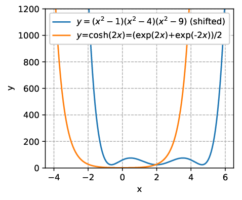
$(L_{0},L_{1})$-smoothness is more realistic than $L$-smoothness. Firstly, it includes a variety of simple and important functions which, unfortunately, do not satisfy $L$-smoothness. For example, all univariate polynomials (which can possibly be non-convex) are $(L_{0},L_{1})$-smooth for $L_{1}=1$, while a simple function $x^{4}$ is not globally $L$-smooth for any $L$. Moreover, $(L_{0},L_{1})$-smoothness also encompasses all functions that belongs to the so-called exponential family. Figure 1(a) presents some simple examples and Figure 1(b) shows that the local smoothness of $(L_{0},L_{1})$-smooth functions strongly correlates to the gradient norm.

Secondly, Zhang et al. 2020a performed experiments to show that $(L_{0},L_{1})$-smoothness is a preciser characterization of the landscapes for objective functions in many real-world tasks, especially for training a deep neural network model. It was observed that the local Lipschitz constant $L_{0}$ near the stationary point is thousands of times smaller than the global one $L$ in the LSTM training (see Figure 1(c) taken from Zhang et al. 2020a).

Seeing this, it is desirable to give a comprehensive and deep analysis on iteration complexities for $(L_{0},L_{1})$-smooth objectives. How fast can we achieve to find a first-order stationary point for $(L_{0},L_{1})$-smooth functions? What are simple algorithms that provably achieve such a convergence rate? In this paper, we give affirmative answers to the above questions. In fact, due to the violent fluctuation of gradients, the efficiency of (stochastic) Gradient Descent with a constant step size degenerates, whereas we will show in this paper that by simply combining the clipping technique, a wide range of algorithms can achieve much better convergence rate for $(L_{0},L_{1})$-smooth functions. In fact, when $\varepsilon$ is small, the complexities (i.e. the number of gradient queries required) are $\mathcal{O}\left(\Delta L_{0}\varepsilon^{-2}\right)$ for the deterministic setting and $\mathcal{O}\left(\Delta L_{0}\sigma^{2}\varepsilon^{-4}\right)$ for the stochastic setting (see Section 3 for details), which are both independent of $L_{1}$. Compared with Zhang et al. 2020a who only studied clipped (stochastic) gradient descent, we consider proposing a unified framework which contains a variety of clipping-based algorithms and achieve much sharper complexities. The main technique for our proof is by introducing a novel Lyapunov function which does not appear in existing studies. We believe that our work provides better understandings for the clipping technique in training deep neural networks. We summarize the contributions of the paper in the following.

• •

  We provide a general framework to analyze the clipping technique for optimizing $(L_{0},L_{1})$-smooth functions. It contains a variety of clipping algorithms, including gradient clipping and momentum clipping as special cases.

• •

  We provide convergence analysis for the general framework we propose. We show that our bounds are tight by comparing with existing lower bounds. For gradient clipping, a special case in our framework, our result is much sharper than that proposed by Zhang et al. 2020a.

• •

  We conduct extensive experiments on a variety of different tasks, and observe that the clipping algorithms consistently perform better than vanilla ones.

Notations. For a vector $x\in\mathbb{R}^{d}$, we denote $\|x\|$ as the $l_{2}$-norm of $x$. For a matrix $A\in\mathbb{R}^{m\times n}$, let $\|A\|$ be the spectral norm of $A$. Given functions $f,g$ : $\mathcal{X}\rightarrow[0,\infty)$ where $\mathcal{X}$ is any set, we say $f=\mathcal{O}(g)$ if there exists a constant $c>0$ such that $f(x)\leq cg(x)$ for all $x\in\mathcal{X}$, and $f=\Omega(g)$ if there exists a constant $c>0$ such that $f(x)\geq cg(x)$ for all $x\in\mathcal{X}$. We say $f=\Theta(g)$ if $f=\mathcal{O}(g)$ and $f=\Omega(g)$.

We aim to present a general framework in which we can provide a unified analysis for commonly used clipping-based algorithms. Since momentum is one of the most popular acceleration technique in optimization community, our framework takes this acceleration procedure into account. We show our framework in Algorithm 1, where we can simply replace $\nabla f(x_{t},\xi_{t})$ by $\nabla F(x_{t})$ for the deterministic setting.

We notice that our framework is similar to the Quasi-Hyperbolic Momentum(QHM) algorithm proposed by Ma and Yarats 2018, while they did not consider the clipping technique. They pointed out that QHM contains a wide range of popular algorithms (e.g. SGD+momentum, Nesterov Accelerated SGD, AccSGD, etc). As a result, for different choice of hyper-parameters, our framework encompasses the clipping version of all these algorithms. We now discuss several representative examples in our framework.

• •

  Gradient Clipping. By choosing $\nu=0$ in Algorithm 1, we obtain the clipped GD/SGD algorithm which can be written as:

  $$x_{t+1}\leftarrow x_{t}-\min\left(\eta,{\gamma}/{\|\nabla f(x_{t},\xi_{t})\|}\right)\nabla f(x_{t},\xi_{t})$$

  It follows that in gradient clipping, the gradient is clipped to have its norm no more than $\gamma/\eta$.

• •

  Momentum Clipping. By choosing $\nu=1$ in Algorithm 1, we perform the update using a clipped version of momentum which can be written as:

  $$x_{t+1}\leftarrow x_{t}-\min\left(\eta,{\gamma}/{\|m_{t+1}\|}\right)m_{t+1}$$

  The approach has already been used in previous works (Zhang et al. 2019; Zhang et al. 2020b), albeit in different settings. To the best of our knowledge, there is no existing analysis of this algorithm even for optimizing standard $L$-smooth functions.

• •

  Mixed Clipping. By choosing $\nu\in(0,1)$, we obtain the mixed clipping algorithm. Although this form of clipping is not widely used in practice, we observe from experiments that it typically converges faster than both gradient clipping and momentum clipping. Some explanations of this observation are provided in Appendix E.

• •

  Normalized Momentum. By choosing $\nu=1$ and $\eta\rightarrow+\infty$ in Algorithm 1, we recover the normalized SGD+momentum algorithm. This algorithm performs a normalized (rather than clipped) update in each iteration. It has been analyzed in Cutkosky and Mehta 2020 for $L$-smooth functions and a layer-wise variant was used in the LARS algorithm (You et al. 2017). We will provide a detailed discussion of this algorithm in the Appendix C.

We conduct extensive experiments and find the clipping algorithms indeed consistently outperform their unclipped counterpart. We present experimental results on three deep learning benchmarks: CIFAR-10 classification using ResNet-32, Imagenet classification using ResNet-50 and language modeling on Penn Treebank (PTB) dataset using AWD-LSTM. We put all the experimental details in the Appendix G. Our code is available at https://github.com/zbh2047/clipping-algorithms.

CIFAR-10 classification with ResNet. We train the standard ResNet-32 (He et al. 2016) architecture on CIFAR-10. We use SGD with momentum for the baseline algorithm with a decaying learning rate schedule, which is the standard choice to train the ResNet architecture. We set learning rate $\eta=1.0$, momentum $\beta=0.9$ and minibatch size 128, following the common practice. For all the clipping algorithms, we choose the best $\eta$ and $\gamma$ based on a course grid search, while keeping other hyper-parameters and training strategy the same as SGD+momentum. We simply set the hyper-parameters $\nu=0.7$ and $\beta=0.999$ in mixed clipping, as suggested in Ma and Yarats 2018 (for its unclipped counterpart QHM). We run 5 times for each algorithm using different random seeds to make the results more reliable.

Figures 2(a) demonstrates the results. It can be seen that all the algorithms achieve a test accuracy more than 93% on CIFAR-10. Note that all clipping algorithms converge faster than SGD+momentum. Particularly, the mixed clipping (Algorithm 1) outperforms SGD+momentum by a large margin in term of training speed. As a result, one can possibly adopt a more aggressive learning rate decaying schedule to reduce training time considerably.

ImagNet classification with ResNet. We train the standard ResNet-50 (He et al. 2016) architecture on ImageNet. For the baseline algorithm, we choose SGD with learning rate $lr=1.0$ and momentum $\beta=0.9$, following Goyal et al. 2017. We use batch size 256 on 4 GPUs.

Figure 2(b) plot the training loss curve and validation accuracy curve on ImageNet. All the algorithms reach a validation accuracy of about 76%. However, all the clipping algorithms train faster than the baseline SGD. Mixed clipping performs the best among the four algorithms.

Language modeling with LSTM. We train the state-of-the-art AWD-LSTM (Merity et al. 2017) on Penn Treebank (PTB) dataset (Mikolov et al. 2010). We first follow the training strategy in Merity et al. 2017, where they use averaged SGD without momentum with learning rate $\eta=30$ and clipping parameter $\gamma=7.5$. Since our purpose is to compare different algorithms rather than to achieve state-of-the-art results, we only train AWD-LSTM for 250 epochs. We then evaluate other algorithms including standard SGD without clipping, momentum clipping, and mixed clipping. We choose the best $\eta$ and $\gamma$ (using validation perplexity criterion) based on a course grid search. Results are shown in Figure 2(c).

Figure 2(c) clearly shows all clipping methods converge much faster than SGD without clipping, and are much better in term of validation perplexity. This is consistent with our theory, in that the vanilla SGD must use a very small learning rate to guarantee convergence (Zhang et al. 2020a), which will be slow and be harmful to generalization on validation set according to previous works (Huang et al. 2017; Kleinberg et al. 2018) . Therefore clipping technique is crucial in LSTM models. We can also find that the training and test curve of mixed clipping is much better than both gradient clipping and momentum clipping. The mixed clipping improves validation perplexity for more than 1 point compared to clipped SGD after 250 epochs.

Other experiments. We also conduct experiments to compare clipping algorithms with Adam, and to directly compare our work with previous results (Zhang et al. 2020a) under the same setting. See Appendix H for details. Finally, we construct a provably $(L_{0},L_{1})$-smooth optimization problem using MNIST dataset. We then run experiments in both deterministic setting and stochastic setting. The results are shown in Appendix I.

This paper proposes a detailed study for clipping methods under a general framework. In particular, we explore the possibility of combining clipping with other popular techniques, e.g. momentum acceleration, in deep learning. We provide a general and tight analysis for the framework, showing the efficiency of clipping methods in optimizing a class of non-convex and non-smooth (in traditional sense) functions. Experiments confirm that these methods have superior performance. We hope that our work affords more understandings on the clipping technique and $(L_{0},L_{1})$ smooth functions.

There are still many open questions that have not yet been answered. Firstly, as discussed in Section 3.3, we are not aware of any lower bounds for general first-order methods that can be applied our setting. Thus, it is interesting to explore such lower bound, or to relax Assumption 2.4 to the more general bounded variance assumption. Secondly, although we have shown the superiority of clipping-based methods, we do not provide theoretical explanation why some clipping schemes are better than others as observed in experiments. We believe that this can only be done by exploring new and better smoothness assumptions. Thirdly, the empirical superiority of other adaptive methods ( e.g. AdaGrad (Duchi et al. 2011), Adam (Kingma and Ba 2014) ) have not been justified from a theoretical point of view. We hope that our analysis is helpful for the analysis of these methods. Finally, we are looking forward to seeing better optimization algorithms with better convergence properties in future work.

This work was supported by National Key R&D Program of China (2018YFB1402600), Key-Area Research and Development Program of Guangdong Province (No. 2019B121204008)] and Beijing Academy of Artificial Intelligence.

In this section, we prove some important properties of $(L_{0},L_{1})$-smooth functions. These properties will be frequently used in subsequent sections.

We first present a basic lemma without proof.

The following result, Lemma A.2 , is a generalization of Lemma 9 in Zhang et al. 2020a.

References

• Abadi et al. [2016] Martin Abadi, Andy Chu, Ian Goodfellow, H Brendan McMahan, Ilya Mironov, Kunal Talwar, and Li Zhang. Deep learning with differential privacy. In Proceedings of the 2016 ACM SIGSAC Conference on Computer and Communications Security, pages 308–318, 2016.
• Arjevani et al. [2019] Yossi Arjevani, Yair Carmon, John C Duchi, Dylan J Foster, Nathan Srebro, and Blake Woodworth. Lower bounds for non-convex stochastic optimization. arXiv preprint arXiv:1912.02365, 2019.
• Carmon et al. [2019] Yair Carmon, John C Duchi, Oliver Hinder, and Aaron Sidford. Lower bounds for finding stationary points i. Mathematical Programming, pages 1–50, 2019.
• Cutkosky and Mehta [2020] Ashok Cutkosky and Harsh Mehta. Momentum improves normalized sgd. arXiv preprint arXiv:2002.03305, 2020.
• Drori and Shamir [2019] Yoel Drori and Ohad Shamir. The complexity of finding stationary points with stochastic gradient descent. arXiv preprint arXiv:1910.01845, 2019.
• Duchi et al. [2011] John Duchi, Elad Hazan, and Yoram Singer. Adaptive subgradient methods for online learning and stochastic optimization. Journal of machine learning research, 12(7), 2011.
• Fang et al. [2018] Cong Fang, Chris Junchi Li, Zhouchen Lin, and Tong Zhang. Spider: Near-optimal non-convex optimization via stochastic path-integrated differential estimator. In Advances in Neural Information Processing Systems, pages 689–699, 2018.
• Ghadimi and Lan [2013] Saeed Ghadimi and Guanghui Lan. Stochastic first-and zeroth-order methods for nonconvex stochastic programming. SIAM Journal on Optimization, 23(4):2341–2368, 2013.
• Goodfellow et al. [2016] Ian Goodfellow, Yoshua Bengio, and Aaron Courville. Deep learning. MIT press, 2016.
• Gorbunov et al. [2020] Eduard Gorbunov, Marina Danilova, and Alexander Gasnikov. Stochastic optimization with heavy-tailed noise via accelerated gradient clipping. arXiv preprint arXiv:2005.10785, 2020.
• Goyal et al. [2017] Priya Goyal, Piotr Dollár, Ross Girshick, Pieter Noordhuis, Lukasz Wesolowski, Aapo Kyrola, Andrew Tulloch, Yangqing Jia, and Kaiming He. Accurate, large minibatch sgd: Training imagenet in 1 hour. arXiv preprint arXiv:1706.02677, 2017.
• Gronwall [1919] T. H. Gronwall. Note on the derivatives with respect to a parameter of the solutions of a system of differential equations. Annals of Mathematics, 20(4):292, 1919.
• He et al. [2016] Kaiming He, Xiangyu Zhang, Shaoqing Ren, and Jian Sun. Deep residual learning for image recognition. In Proceedings of the IEEE conference on computer vision and pattern recognition, pages 770–778, 2016.
• Huang et al. [2017] Gao Huang, Yixuan Li, Geoff Pleiss, Zhuang Liu, John E Hopcroft, and Kilian Q Weinberger. Snapshot ensembles: Train 1, get m for free. arXiv preprint arXiv:1704.00109, 2017.
• Kingma and Ba [2014] Diederik P Kingma and Jimmy Ba. Adam: A method for stochastic optimization. arXiv preprint arXiv:1412.6980, 2014.
• Kleinberg et al. [2018] Bobby Kleinberg, Yuanzhi Li, and Yang Yuan. An alternative view: When does sgd escape local minima? In International Conference on Machine Learning, pages 2698–2707, 2018.
• Levy [2016] Kfir Y Levy. The power of normalization: Faster evasion of saddle points. arXiv preprint arXiv:1611.04831, 2016.
• Ma and Yarats [2018] Jerry Ma and Denis Yarats. Quasi-hyperbolic momentum and adam for deep learning. arXiv preprint arXiv:1810.06801, 2018.
• Menon et al. [2020] Aditya Krishna Menon, Ankit Singh Rawat, Sashank J Reddi, and Sanjiv Kumar. Can gradient clipping mitigate label noise. In International Conference on Learning Representations, 2020.
• Merity et al. [2017] Stephen Merity, Nitish Shirish Keskar, and Richard Socher. Regularizing and optimizing lstm language models. arXiv preprint arXiv:1708.02182, 2017.
• Mikolov [2012] Tomáš Mikolov. Statistical language models based on neural networks. Presentation at Google, Mountain View, 2nd April, 80, 2012.
• Mikolov et al. [2010] Tomáš Mikolov, Martin Karafiát, Lukáš Burget, Jan Černockỳ, and Sanjeev Khudanpur. Recurrent neural network based language model. In Eleventh annual conference of the international speech communication association, 2010.
• Pascanu et al. [2012] Razvan Pascanu, Tomas Mikolov, and Yoshua Bengio. Understanding the exploding gradient problem. CoRR, abs/1211.5063, 2:417, 2012.
• Pascanu et al. [2013] Razvan Pascanu, Tomas Mikolov, and Yoshua Bengio. On the difficulty of training recurrent neural networks. In International conference on machine learning, pages 1310–1318, 2013.
• You et al. [2017] Yang You, Igor Gitman, and Boris Ginsburg. Scaling sgd batch size to 32k for imagenet training. arXiv preprint arXiv:1708.03888, 6, 2017.
• Zhang et al. [2019] Jingzhao Zhang, Sai Praneeth Karimireddy, Andreas Veit, Seungyeon Kim, Sashank J Reddi, Sanjiv Kumar, and Suvrit Sra. Why adam beats sgd for attention models. arXiv preprint arXiv:1912.03194, 2019.
• Zhang et al. [2020a] Jingzhao Zhang, Tianxing He, Suvrit Sra, and Ali Jadbabaie. Why gradient clipping accelerates training: A theoretical justification for adaptivity. In International Conference on Learning Representations, 2020a.
• Zhang et al. [2020b] Jingzhao Zhang, Hongzhou Lin, Suvrit Sra, and Ali Jadbabaie. On complexity of finding stationary points of nonsmooth nonconvex functions. arXiv preprint arXiv:2002.04130, 2020b.
Appendix A  Properties of (L0,L1)(L_{0},L_{1})-smooth functions