Visualizing Color-wise Saliency of
Black-Box Image Classification Models
Abstract
Image classification based on machine learning is being commonly used. However, a classification result given by an advanced method, including deep learning, is often hard to interpret. This problem of interpretability is one of the major obstacles in deploying a trained model in safety-critical systems. Several techniques have been proposed to address this problem; one of which is RISE, which explains a classification result by a heatmap, called a saliency map, that explains the significance of each pixel. We propose MC-RISE (Multi-Color RISE), which is an enhancement of RISE to take color information into account in an explanation. Our method not only shows the saliency of each pixel in a given image as the original RISE does, but the significance of color components of each pixel; a saliency map with color information is useful especially in the domain where the color information matters (e.g., traffic-sign recognition). We implemented MC-RISE and evaluate them using two datasets (GTSRB and ImageNet) to demonstrate the effectiveness of our methods in comparison with existing techniques for interpreting image classification results.
1 Introduction
As machine learning is widely applied to image classification, there is a surging demand for the methods to explain classification results and visualize it. One can use such an explanation to check whether a trained model classifies images based on a rational and acceptable criterion, by which he or she can convince various stakeholders that the model is readily deployed.
One of the most popular ways of the visualization is by a saliency map—a heatmap overlayed on the original image that indicates which part of the image contributes to the classification result [1, 2, 3, 4, 5, 6, 7, 8, 9, 10, 11, 12, 13, 14]. Fig. 1 shows an example of a saliency map generated by a method called RISE [4]. Given the image (a) of a road sign “STOP” and a model that indeed classifies this image as a stop sign, RISE generates the saliency map (b), which indicates the part of (a) that contributes to the classification result by a heatmap. From this saliency map, we can figure out that the part of the sign surrounding the text “STOP” contributes positively to the classification result.
Among the explanation methods proposed so far, model-agnostic techniques such as LIME [1], SHAP [2], and RISE [4] generate a saliency map without accessing the internal information of a model, treating it as a black box. Although these procedures differ in their detail, they all share the following central idea: They compute a saliency map for a classification result by perturbing the given image and observing how the output of the perturbed image changes from the original. Concretely, given an image , a model , and its classification result, they compute a saliency map by (1) generating perturbed image from by masking a part of it, (2) computing the classification result for each perturbed image, and (3) comparing with each . If the output of a perturbed image with a specific part unmasked tends to be the same as , then this part is considered to be important.

Although these model-agnostic explanation techniques give valuable insights about a classification result of an image, there is important information that has been overlooked by these methods: colors. They compute a saliency map indicating each pixel’s existence, but they do not take the color information of a pixel into account. A color-aware explanation is effective especially in the application domains in which the colors in an image convey important information (e.g., traffic-sign recognition).
This paper proposes an extension of RISE [4] so that it generates a color-aware saliency map. We extend the original RISE so that it can compute a saliency map for each color of a given color set; we call our extended method MC-RISE (Multi-Color RISE). Fig. 1 (c) shows the saliency maps generated by MC-RISE. It consists of five heatmaps, each of which corresponds to the significance of a certain color of each pixel; the associated color is shown above each heatmap. We can figure out that the red color at the peripheral part of the stop sign contributes much to the classification result, whereas the other colors do not contribute as much as red.
We also propose an enhancement to debias the original RISE. In our extension, the saliency of the pixels in an input image is close to if it is irrelevant for the classification result. Notice that the heatmaps in Fig. 1 (c) have value close to for the irreverent pixels, whereas the heatmap generated by the original RISE in Fig. 1 (b) does not contain a pixel of value ; it is hard to figure out which part of the image is irreverent to the classification result from the latter saliency map.
The contributions of the paper are summarized as follows. (i) We propose a new model-agnostic explanation method for an image classifier, MC-RISE, which generates color-aware saliency maps for the classifier’s decision. (ii) To improve the interpretability of the saliency map, we propose a method to debias the saliency map of RISE and incorporate it into MC-RISE. (iii) We qualitatively and quantitatively compare our method to existing model-agnostic explanation methods (LIME [1] and RISE [4]) in GTSRB [15] dataset and ImageNet [16] dataset, and showed that our method can extract additional information which can not be obtained by the existing methods, such as color-sensitivity.
2 Related Work
Explanation-generating methods for an image classifier proposed so far can be categorized into the following two groups: (1) ones that treat a model as a black box and (2) ones that treat a model as a white box. The former observes the input–output relation in generating an explanation without using the internal information of a model; whereas the methods in the latter group assume that the internal information is accessible. As far as we know, our method is the first explanation-generating method for black-box models that considers color information in generating an explanation.
Many white-box methods compute a saliency map utilizing the classifier’s gradient information. Grad-CAM [5] and its extension Grad-CAM++ [6] use the gradient with respect to an intermediate feature map to obtain class-specific weights for the feature map. Integrated gradient [7] and SmoothGrad [8] accumulate the gradients with respect to modified input images in order to get a more interpretable sensitivity map than a single gradient map. In [9, 10, 11, 12, 13], the relevance map for an intermediate layer is back-propagated layer-by-layer from the output layer to the input layer with a modified back-propagation rule.
However, it is pointed out that the explanation generated by gradient-based methods are not necessarily faithful to the classifier’s decision process. Adebayo et al. [17] shows that some gradient-based methods are nearly independent of the classifier’s weight, and act like a model-ignorant edge detector rather than an explanation of the classifier. [18, 19, 20] adversarially attack gradient-based methods and can manipulate a saliency map without regard to the classifier’s output. From these results, we expect that the methods based on the input–output relation are more faithful to the classifier’s actual behavior than gradient-based methods.
Other white-box methods include optimization-based methods and attention-based methods. In Meaningful perturbation [21], Extremal Perturbations [22], and FGVis [23], the image region to add perturbation (e.g. blurring, masking) are optimized by gradient descent with respect to an input image, and saliency information is extracted from the perturbed region. In [24], a visual question answering model with the attention mechanism is proposed and the attention maps can be interpreted as the relevant parts in an image.
LIME (Local Interpretable Model-agnostic Explanation) [1] and SHAP [2] are popular explanation-generating methods for a black-box image-classifier. Both perturb the given image preprocessed into a set of superpixels, observe how the output to the perturbed image, and generate an explanation based on the change in the output. Although their merits are widely appreciated, it is known that a generated explanation is not robust to how an image is decomposed into superpixels [25]. Our extension proposed in this paper is based on RISE [4] instead, which does not require a prior preprocessing of an input image. We will explain RISE in detail in §3.
Some black-box methods are based on these black-box techniques. IASSA [14] is an extension of RISE, which refines a saliency map by iteratively adapting the mask sampling process based on the previous saliency map and attention map. As extensions of the LIME framework, LORE [26] generates sample data with a genetic algorithm and fits decision trees instead of the linear regression model in LIME, and [27] incorporates the effect of higher-order interactions between input features.
3 RISE
This section explains an explanation-generating method RISE [4], which is the basis of our method. For a detailed exposition, see Petsiuk et al. [4].
We first designate several definitions to define RISE. An image is a mapping from a finite set of pixels to . For an image and a pixel , the tuple is the RGB value of in . We write for the set of images. We also designate the finite set of labels . We fix an image-classification model throughout this paper; is the model confidence in classifying as . For any , we assume that .
A mask is an element of . A mask represents an image transformation that sets the RGB value of a pixel to if ; the transformation keeps the original value of if Therefore, the image that is obtained by applying the image transformation to an image is defined by .
Given an image and a label , we define the saliency map as , where the expectation is taken over all the possible masks. The intuition behind this definition is that can be considered to positively contribute to the classification of to if the model confidence of classifying the image to remains high when is not masked.
Let be a random variable whose value is a mask. Then, the definition of is equal to
| (1) |
This expression shows that we can compute by computing the model confidence for every mask that does not mask and taking the weighted sum of these values.
Remark 1
In the actual implementation of RISE, the following optimizations are often applied.
- •
It is prohibitively expensive to precisely computing the value of the expression (1). Therefore, is approximated by the Monte-Carlo method. We randomly sample sufficiently many masks and compute
(2) Here, is , is the -th mask, and is the number of samples.
- •
RISE preprocesses a mask by bilinear interpolation before it applies the mask to an image. This is based on the intuition that (1) the saliency of a pixel is not binary and (2) a pixel that is close to an important pixel is often important. After this optimization, a mask is an element of instead of .
Our extensions proposed in this paper also uses these optimizations.
4 Debiased RISE and MC-RISE
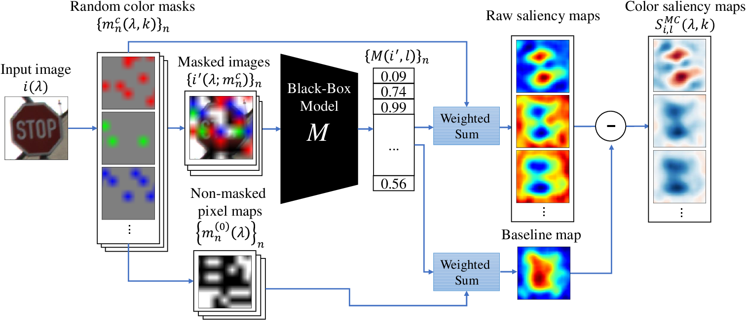
This section describes our extension to RISE. As we mentioned in §1, our extension consists of two enhancements of RISE: (1) MC-RISE, which generates color-aware saliency maps, and (2) debiasing saliency maps, which is a tweak to the RISE procedure so that the value of an irrelevant pixel in a saliency map is close to . We first present (2) in §4.1 and then (1) in §4.2.
4.1 Removing Bias from Saliency Maps
The range of the saliency values of a heatmap generated by RISE is highly variable depending on an input image. For example, the values in the saliency map at the first row in Fig. 4 (c) ranges from to , whereas the one at the third row ranges from to . This variability of saliency values degrades interpretability because it makes thresholding saliency value difficult: There is no clear threshold to decide which pixel is positively important, which is negatively important, and which is irrelevant.
To address this problem, we tweak the definition of RISE so that the saliency value of an irrelevant pixel to be close to , a positively-important pixel to be positive, and a negatively-important pixel to be negative; in other words, our method generates a debiased saliency map. Concretely, we generate a saliency map using the following definition instead of Equation (1):
| (3) |
Intuition behind Equation (3) is that we also need to use negative saliency of a pixel for the classification result in computing a saliency map, not only using the positive saliency as RISE does. The expression indeed expresses the negative saliency of because its value becomes high if masking out the pixel increases the model confidence on average over the masks. To give the saliency as a single number, we calculate the difference of the positive saliency and the negative saliency. As a result, the sign of indicates whether positive or negative saliency is dominant at a given pixel .
Calculating the difference of the positive saliency and the negative saliency also makes the saliency value of an irrelevant pixel to be . We can prove that a saliency map generated from Equation (3) is equipped with the following property (for the proof, see Appendix 0.C):
Proposition 1 (Irrelevant pixels)
If, for all binary mask samples, the output probability of class from a black-box classifier does not vary no matter whether a pixel in the mask is retained or masked (i.e. ), then .
This property justifies the following interpretation of : A pixel whose value of is close to has almost no effect on the classification result. It is worth noting that (1) the sign of the value of carries information on whether the pixel positively/negatively significant for the classification of to and (2) its absolute value expresses how significant is for the classification. In the original RISE, we can observe only that is more/less positively significant than another pixel in the image if the value of is larger/smaller than . In §5.2, we empirically justify the above interpretation and argue that these properties render the interpretation of our saliency map easier than the one of the original RISE.
Equation (3) can be rewritten to the following equation that computes by a weighted sum over all masks (see Appendix 0.A for the detailed derivation):
| (4) |
where . We approximate by Monte Carlo sampling and express it by the following equation:
| (5) |
where is the number of mask samples and are randomly-sampled masks. We remark that Equation (5) is obtained from Equation (2) simply by replacing with ; therefore, we can easily implement our debiasing method by modifying the implementation of RISE.
4.2 Multi-Colored RISE (MC-RISE)
We next present MC-RISE, our extension to RISE that explains the color-wise saliency of each pixel. The main idea of MC-RISE is to use a colored mask instead of a binary mask that RISE uses. Then, we can compute the positive/negative saliency of the given color component of a pixel from the response of the model to the masked image. The pseudocode for MC-RISE is presented in Appendix 0.F.
Color Masks
We explain the method to generate color masks and color-masked images in MC-RISE. We fix a set of colors where each is a 3-tuple of color values in the RGB colorspace. We are to generate a saliency map for each . To this end, MC-RISE generates colored masks instead of the binary masks that RISE uses. The saliency map is computed from the change in the average model confidence for the color-masked image in a similar way to RISE. We will explain the details of the saliency-map computation later.
To generate a colored mask, MC-RISE first generates a low-resolution color mask of the size (which is smaller than the input image’s size), where is the position of a pixel and is the index for masking color in the color set . The low-resolution color mask is generated as follows:
- 1.
For each pixel, MC-RISE randomly decides whether it is masked or not with a masking probability .
- 2.
For each pixel that is decided to be masked, MC-RISE chooses the color used to mask it from the color set with the uniform probabilities.
- 3.
Then, the color mask is defined as follows:
(6)
Then, is converted to a high-resolution color mask by (1) resizing to the size of input images using bilinear interpolation and (2) shifting the resized mask by a random number of pixels from up to (i.e., the size of a low-resolution pixel). We remark that the computation of corresponds to the preprocessing of a mask in RISE mentioned in Remark 1.
We also compute a non-masked pixel map by
| (7) |
is for non-masked pixels and for masked pixels.
From a color mask and an input image , the color-masked image is computed by . Because of Equations (6) and (7), this expression can be seen as the alpha blending of an input image and the images uniformly filled with the masking colors .
In Fig. 2, an example of a color mask , a non-masked pixel map , and a color-masked image are presented.
Color-aware Saliency Map
The saliency map of MC-RISE is defined by
| (8) | |||||
where denotes the probability distribution of color masks induced by the above mask-generation procedure. represents how sensitively the model’s confidence in classifying an image to class responds when the pixel in an input image is masked by the color .
The debiasing method of a saliency map discussed in Section 4.1 is incorporated also into the definition of color saliency maps (Equation (8)), where the baseline saliency map for non-masked pixels (, corresponding to the effect of retaining the pixel ) is subtracted from the raw saliency maps (, corresponding to the effect of masking the pixel ).
The formula to estimate a color saliency map with Monte Carlo sampling can be derived in a similar way to §4.1 (see Appendix 0.B for the detailed derivation);
| (9) | |||||
where is the number of mask sampling and are color masks sampled from the distribution . In our implementation, and in Equation (9) are separately accumulated using the same samples of color masks ; is computed by subtracting the weighted-sum of the second term (baseline map) from that of the first term (raw saliency maps), as illustrated in Fig. 2.
Interpretation of Color Saliency Maps
Since the debiasing method of §4.1 is incorporated into the definition of color saliency maps (Equation (8)), we can interpret the sign of a color saliency map as a positive/negative effect on the decision given by the model as we discussed in §4.1. However, because the sign of a color saliency map represents the expected change in the model confidence by color-masking a pixel , the interpretation of the sign of a saliency value is different from the debiased RISE in §4.1, in which a saliency value represents the effect of retaining original pixels. Therefore, we can interpret the color saliency map as follows:
- •
If has a positive or negative value for all , the model’s output probability of class should increase or decrease by any kind of color mask at a pixel , respectively. This suggests that the original texture at pixel is an obstacle or an important feature to the model, respectively, and its overall color is not relevant to the model’s decision.
- •
If for all , any kind of masking at the pixel should not affect the model’s output. It means that the pixel is irrelevant to the model’s decision.
- •
If for some , the model’s output probability of class should increase by masking the pixel with the color . This indicates that the presence of the color at the pixel is an important feature for the model to classify an image as class , but the original image lacks this feature.
- •
If for some , the model’s output probability of class should decrease by masking the pixel with the color . This suggests that the pixel ’s original color is an influential feature for the model to classify an image as class and masking it with the color degrade the model’s confidence for class .
- •
If for some , color-masking the pixel with the color should not affect the model’s output. It suggests that the color is similar to the original color of the pixel from the viewpoint of the model, therefore masking with other colors would affect the model’s output.
5 Experiments
5.1 Experimental Settings
We use LIME [1] and RISE [4] as the baseline for the evaluation of our methods. We designated two kinds of models trained with different datasets for the evaluation.
- •
Models trained with GTSRB [15] dataset: We trained (1) VGG-16 [30] model with batch normalization and (2) ResNet-50 [31] model. We trained the models for epochs with momentum SGD using cross-entropy loss. We set the learning rate to , the momentum to , and the weight decay to ; we decayed the learning rate by a factor of in every epochs. We resized images to pixels for training and evaluation.
- •
For MC-RISE and RISE, the number of samples was set to and the masking probability was set to . For MC-RISE, we used the following five colors: red ( in the RGB colorspace), green (), blue (), white (), and black (). For LIME, the parameters that we used were the same as the original paper [1].
We also applied MC-RISE to a person re-identification model with metric learning. See Appendix 0.D for details.
5.2 Results
Qualitative Evaluation of the Debiasing Method

We qualitatively evaluated the debiasing method presented in §4.1. Fig. 3 compares the saliency maps of RISE and our debiased saliency map; we used ImageNet dataset to generate these maps. In the saliency map generated by the original RISE (Fig. 3(b)), the saliency values of the background regions—which should be irrelevant to the decision of the model—largely differs depending on the input images both in their absolute values and in their relative magnitude (i.e., pseudo-color in the plots). In our debiased maps (Fig. 3(c)), the background regions of all the images have the saliency values that are close to zero. These results demonstrate that the debiased RISE computes a saliency map in which the saliency values of the irrelevant regions are close to zero as we intend.
The saliency maps on the second and third rows in Fig. 3(c) shows that the saliency values near the objects of the output class (i.e., Drum and Suit) are positive and that the saliency values near the “noisy” objects (i.e., heart-shaped weight and necktie) are negative. These behaviors are also in accordance with the interpretation we presented in §4.1.
Qualitative Evaluation of MC-RISE

Fig. 4 compares saliency maps generated by LIME [1], RISE [4], and our method MC-RISE; we used GTSRB dataset to generate these saliency maps. The saliency values of MC-RISE on the third row are not sensitive to the colors (i.e. the sign and the values of is similar for all ). As we mentioned in §4.2, this suggests that the texture information is important for the model than the color information.
The saliency map of the image on the first row in Fig. 6 is sensitive to colors. In this image, the saliency near the white arrow is negative for all the colors; this suggests that the texture of this region (i.e., the arrow shape) is important for the model. In contrast, the values near the peripheral region of the sign in the green and the blue saliency maps are positive; this suggests that the blue-like color of this region is important for the model’s decision. Notice that LIME nor RISE can detect the sensitivity to colors; in fact, these parts identified as salient in the green and the blue saliency maps are not necessarily identifiable in the saliency maps generated by LIME and RISE.

Fig. 5 shows the comparison of the saliency maps in ImageNet dataset. Compared to maps in the GTSRB dataset, many of the maps in the ImageNet dataset have low color-dependency among the color saliency maps. This suggests that the model’s decision is more dependent on the detailed texture of objects than on the color of image regions. In such cases, we can extract information about positive or negative saliency from the color saliency maps. For example, in the third-row samples in Fig. 5, color saliency maps are interpreted to mean that the upper part of the image is important for the classification output (“Mobile home” class), but the fences in the lower part of the image are reducing the model’s confidence for the output class. From these observations, it is expected that MC-RISE can extract more useful information in domains where the color in image regions is highly important for classification, such as the GTSRB dataset, than domains where detailed texture is important such as the ImageNet dataset.
Quantitative Evaluation of MC-RISE
| Dataset | Model | LIME | RISE | MC-RISE |
|---|---|---|---|---|
| GTSRB | VGG-16 | 0.1324 | 0.0664 | 0.0270 |
| ResNet50 | 0.1294 | 0.0627 | 0.0204 | |
| ImageNet | ResNet50 | 0.1146 | 0.1046 | 0.0980 |
For the quantitative evaluation of MC-RISE, we first would like to establish the evaluation metrics we use. We adapt the deletion metric proposed by Petsiuk et al. [4]—which measures how well a saliency-map–based explanation of an image classification result localizes the important pixels—to our color-aware setting.
To explain the deletion metric, let be an image and be a model. The deletion metric is the AUC value of the plot of where is the model confidence of the image in which the 1st to the -th important pixels are removed. The lower the deletion metric is, the better the saliency map localizes the important region; a lower metric value means that the model confidence drops rapidly because the saliency map successfully points out the important pixels.
Our metric, called CA-deletion (color-aware deletion) is derived from the deletion metric as follows. In the CA-deletion metric, pixels in an input image are removed by masking them with the most sensitive color obtained from the color saliency maps. Concretely, pixel is removed in the ascending order of and the removed pixel is filled by the color where . The model confidence for the pixel-removed images are plotted against the pixel-removal fractions; the CA-deletion value is the area-under-curve (AUC) of the plot. If a color saliency map correctly captures the model’s sensitivity to color masking, this removal method must be effective to reduce the model confidence, resulting in a low value of the CA-deletion metric.11 1 Notice that other common metrics (e.g., pointing game) are not appropriate for evaluating MC-RISE because these metrics focus on the positional saliency; they do not consider the color saliency.
Table 1 shows the evaluation result of MC-RISE in comparison with LIME and RISE. MC-RISE consistently outperforms RISE and LIME especially by a large margin in the GTSRB dataset. This indicates that MC-RISE can correctly capture the color-dependent sensitivity of the model, and effectively localize important pixels in an input image by using this information. The large margin in the GTSRB dataset is in accordance with our expectation that MC-RISE is especially effective in a domain, such as traffic sign classification, where color information conveys important information.
Use Case: Error Analysis Using MC-RISE

We demonstrate a use case of MC-RISE for analyzing misclassified samples. Fig. 6 shows the color saliency maps generated by MC-RISE for a sample in GTSRB dataset that is misclassified by our model. The input is an image of a “Priority road” sign, whereas our model misclassified it as a “No vehicles” sign.
The saliency maps for the output “No vehicles” class show that the colors other than white at the center part of the sign have a negative effect in classifying this image as “No vehicles”. This suggests that, if the color of the center part were not white, then this image would not be classified as “No vehicles” class.
In contrast, in the saliency maps of the GT class (i.e., “Priority road” sign), the saliency map for red color has a strong positive value at the center of the sign, suggesting that the confidence of “Priority Road” class would largely increase if the color of the central part were red. From the above observations, we can hypothesize that the cause of the error is the absence of red color at the center of the sign (possibly due to overexposure). As one can observe, the information obtained by MC-RISE in addition to that obtained by the other methods, such as color-sensitivity or negative saliency, is indeed useful to explore the cause of the misclassification, especially when there is no objects which clearly hinder the correct decision of the model in an input image.
6 Conclusion
We proposed two extensions of a model-agnostic interpretation method RISE [4]. One is debiased RISE; it computes a saliency map in which the saliency of an unimportant pixel is close to ; this makes the interpretation of a saliency map easier than RISE. Another is MC-RISE, which computes color-wise saliency; a saliency map for a color computed by MC-RISE explains the saliency of the color in each pixel. Such color-wise saliency is useful in application domains such as road sign recognition, in which colors convey significant information. We empirically demonstrated the effectiveness of our extensions.
We plan to extend our idea to use other features than colors; for example, by using masks that blur a part of an image, we expect that we can generate a saliency map that explains the significance of the clarity of the region.
Acknowledgment
We thank the reviewers for their fruitful comments.
References
- [1] Ribeiro, M.T., Singh, S., Guestrin, C.: ”why should I trust you?”: Explaining the predictions of any classifier. In: SIGKDD 2016. (2016)
- [2] Lundberg, S.M., Lee, S.I.: A unified approach to interpreting model predictions. In: NIPS 2017. (2017)
- [3] Selvaraju, R.R., Cogswell, M., Das, A., Vedantam, R., Parikh, D., Batra, D.: Grad-cam: Visual explanations from deep networks via gradient-based localization. In: ICCV 2017. (2017)
- [4] Petsiuk, V., Das, A., Saenko, K.: RISE: randomized input sampling for explanation of black-box models. In: BMVC 2018. (2018)
- [5] Selvaraju, R.R., Cogswell, M., Das, A., Vedantam, R., Parikh, D., Batra, D.: Grad-CAM: Visual Explanations from Deep Networks via Gradient-Based Localization. In: 2017 IEEE International Conference on Computer Vision (ICCV). (2017) 618–626 ISSN: 2380-7504.
- [6] Chattopadhay, A., Sarkar, A., Howlader, P., Balasubramanian, V.N.: Grad-CAM++: Generalized Gradient-Based Visual Explanations for Deep Convolutional Networks. In: 2018 IEEE Winter Conference on Applications of Computer Vision (WACV). (2018) 839–847
- [7] Sundararajan, M., Taly, A., Yan, Q.: Axiomatic attribution for deep networks. In: Proceedings of the 34th International Conference on Machine Learning - Volume 70. ICML’17, Sydney, NSW, Australia, JMLR.org (2017) 3319–3328
- [8] Smilkov, D., Thorat, N., Kim, B., Viégas, F., Wattenberg, M.: SmoothGrad: removing noise by adding noise. arXiv preprint (2017) arXiv:1706.03825 arXiv: 1706.03825.
- [9] Zeiler, M.D., Fergus, R.: Visualizing and Understanding Convolutional Networks. In Fleet, D., Pajdla, T., Schiele, B., Tuytelaars, T., eds.: Computer Vision – ECCV 2014. Lecture Notes in Computer Science, Cham, Springer International Publishing (2014) 818–833
- [10] Springenberg, J., Dosovitskiy, A., Brox, T., Riedmiller, M.: Striving for Simplicity: The All Convolutional Net. In: International Conference on Learning Representations. (2015)
- [11] Bach, S., Binder, A., Montavon, G., Klauschen, F., Müller, K.R., Samek, W.: On Pixel-Wise Explanations for Non-Linear Classifier Decisions by Layer-Wise Relevance Propagation. PLOS ONE 10 (2015) e0130140 Publisher: Public Library of Science.
- [12] Shrikumar, A., Greenside, P., Kundaje, A.: Learning Important Features Through Propagating Activation Differences. In Precup, D., Teh, Y.W., eds.: Proceedings of the 34th International Conference on Machine Learning. Volume 70 of Proceedings of Machine Learning Research., International Convention Centre, Sydney, Australia, PMLR (2017) 3145–3153
- [13] Zhang, J., Bargal, S.A., Lin, Z., Brandt, J., Shen, X., Sclaroff, S.: Top-Down Neural Attention by Excitation Backprop. Int J Comput Vis 126 (2018) 1084–1102
- [14] Vasu, B., Long, C.: Iterative and Adaptive Sampling with Spatial Attention for Black-Box Model Explanations. In: The IEEE Winter Conference on Applications of Computer Vision. (2020) 2960–2969
- [15] Stallkamp, J., Schlipsing, M., Salmen, J., Igel, C.: Man vs. computer: Benchmarking machine learning algorithms for traffic sign recognition. Neural Networks 32 (2012)
- [16] Russakovsky, O., Deng, J., Su, H., Krause, J., Satheesh, S., Ma, S., Huang, Z., Karpathy, A., Khosla, A., Bernstein, M., Berg, A.C., Fei-Fei, L.: ImageNet Large Scale Visual Recognition Challenge. Int J Comput Vis 115 (2015) 211–252
- [17] Adebayo, J., Gilmer, J., Muelly, M., Goodfellow, I., Hardt, M., Kim, B.: Sanity Checks for Saliency Maps. In Bengio, S., Wallach, H., Larochelle, H., Grauman, K., Cesa-Bianchi, N., Garnett, R., eds.: Advances in Neural Information Processing Systems 31. Curran Associates, Inc. (2018) 9505–9515
- [18] Heo, J., Joo, S., Moon, T.: Fooling Neural Network Interpretations via Adversarial Model Manipulation. In Wallach, H., Larochelle, H., Beygelzimer, A., Alché-Buc, F.d., Fox, E., Garnett, R., eds.: Advances in Neural Information Processing Systems 32. Curran Associates, Inc. (2019) 2925–2936
- [19] Dombrowski, A.K., Alber, M., Anders, C., Ackermann, M., Müller, K.R., Kessel, P.: Explanations can be manipulated and geometry is to blame. In Wallach, H., Larochelle, H., Beygelzimer, A., Alché-Buc, F.d., Fox, E., Garnett, R., eds.: Advances in Neural Information Processing Systems 32. Curran Associates, Inc. (2019) 13589–13600
- [20] Subramanya, A., Pillai, V., Pirsiavash, H.: Fooling Network Interpretation in Image Classification. In: Proceedings of the IEEE International Conference on Computer Vision. (2019) 2020–2029
- [21] Fong, R.C., Vedaldi, A.: Interpretable Explanations of Black Boxes by Meaningful Perturbation. In: Proceedings of the IEEE International Conference on Computer Vision. (2017) 3429–3437
- [22] Fong, R., Patrick, M., Vedaldi, A.: Understanding deep networks via extremal perturbations and smooth masks. In: ICCV 2019. (2019)
- [23] Wagner, J., Kohler, J.M., Gindele, T., Hetzel, L., Wiedemer, J.T., Behnke, S.: Interpretable and Fine-Grained Visual Explanations for Convolutional Neural Networks. In: Proceedings of the IEEE Conference on Computer Vision and Pattern Recognition. (2019) 9097–9107
- [24] Xu, K., Ba, J., Kiros, R., Cho, K., Courville, A., Salakhudinov, R., Zemel, R., Bengio, Y.: Show, Attend and Tell: Neural Image Caption Generation with Visual Attention. In: International Conference on Machine Learning. (2015) 2048–2057 ISSN: 1938-7228 Section: Machine Learning.
- [25] Schallner, L., Rabold, J., Scholz, O., Schmid, U.: Effect of superpixel aggregation on explanations in LIME — A case study with biological data. CoRR abs/1910.07856 (2019)
- [26] Guidotti, R., Monreale, A., Ruggieri, S., Pedreschi, D., Turini, F., Giannotti, F.: Local Rule-Based Explanations of Black Box Decision Systems. arXiv preprint (2018) arXiv:1805.10820 arXiv: 1805.10820.
- [27] Tsang, M., Cheng, D., Liu, H., Feng, X., Zhou, E., Liu, Y.: Feature Interaction Interpretability: A Case for Explaining Ad-Recommendation Systems via Neural Interaction Detection. In: International Conference on Learning Representations. (2019)
- [28] Ribeiro, M.T., Singh, S., Guestrin, C.: Anchors: High-Precision Model-Agnostic Explanations. In: Thirty-Second AAAI Conference on Artificial Intelligence. (2018)
- [29] Schwab, P., Karlen, W.: CXPlain: Causal Explanations for Model Interpretation under Uncertainty. In Wallach, H., Larochelle, H., Beygelzimer, A., Alché-Buc, F.d., Fox, E., Garnett, R., eds.: Advances in Neural Information Processing Systems 32. Curran Associates, Inc. (2019) 10220–10230
- [30] Simonyan, K., Zisserman, A.: Very deep convolutional networks for large-scale image recognition. arXiv preprint arXiv:1409.1556 (2014)
- [31] He, K., Zhang, X., Ren, S., Sun, J.: Deep residual learning for image recognition. In: CVPR 2016. (2016)
- [32] Paszke, A., Gross, S., Massa, F., Lerer, A., Bradbury, J., Chanan, G., Killeen, T., Lin, Z., Gimelshein, N., Antiga, L., Desmaison, A., Kopf, A., Yang, E., DeVito, Z., Raison, M., Tejani, A., Chilamkurthy, S., Steiner, B., Fang, L., Bai, J., Chintala, S.: PyTorch: An Imperative Style, High-Performance Deep Learning Library. In Wallach, H., Larochelle, H., Beygelzimer, A., Alché-Buc, F.d., Fox, E., Garnett, R., eds.: Advances in Neural Information Processing Systems 32. Curran Associates, Inc. (2019) 8026–8037
- [33] Zheng, L., Shen, L., Tian, L., Wang, S., Wang, J., Tian, Q.: Scalable person re-identification: A benchmark. In: Proceedings of the IEEE International Conference on Computer Vision (ICCV). (2015)
- [34] Zhou, K., Yang, Y., Cavallaro, A., Xiang, T.: Omni-scale feature learning for person re-identification. In: Proceedings of the IEEE/CVF International Conference on Computer Vision (ICCV). (2019)
- [35] Zhou, K., Xiang, T.: Torchreid: A library for deep learning person re-identification in pytorch. arXiv preprint arXiv:1910.10093 (2019)
Appendix 0.A Derivation of Equation (4)
Appendix 0.B Derivation of Equation (9)
Following the similar derivation in §0.A, the definition of (Equation (8)) can be expressed as
| (14) | |||||
In the mask generation process, whether a pixel is masked or retained is randomly determined with the masking probability , and for a masked pixel, the masking color is sampled from the uniform distribution over colors; hence, and . Substituting them in the expression of (Equation (14)) yields Equation (9);
| (15) |
Appendix 0.C Proof of Proposition 1
Let be a fixed pixel and be the set of all possible masks. We define a disjoint partition of by and . From the definition of (Equation (3)), we get
| (16) | |||||
because if and vice versa.
Let be the function which flips the mask value at pixel . induces a one-to-one correspondence between the masks in and . Therefore, Equation (16) is expressed as
| (17) | |||||
We can rewrite as
| (18) | |||||
where is the Kronecker delta and is the masking probability for a pixel. Therefore, Equation (17) is rewritten as
| (19) | |||||
Appendix 0.D Additional Experiments with Person ReID model
This section presents the application of MC-RISE to a metric-learning-based person re-identification (ReID) model.
A metric-learning-based person ReID model takes an image of a person as input and outputs the feature vector for the input image. The model is trained so that, if it is given a pair of images and , then the distance between and is small if and are likely to be the images of the same person. We designate a set of gallery images; at inference time, we compare the feature vector of a query image with those of the gallery images and retrieve a gallery image that belongs to the same person as the query.
We adapted MC-RISE as follows to apply it to a person ReID model.
- •
Unlike a standard classification task where an image belongs to a unique class, a person ReID task has multiple correct gallery images for one query image in general. In this experiment, we only consider the gallery image of the top-1 match to a query image as the correct label; the feature distance to the top-1 match image is used as the output of the black-box model , that is used by MC-RISE. Hence, MC-RISE visualizes how the similarity to the top-1 match image responds to the color masking of an input image.
- •
As for the definition of feature distance, the simple Euclidean distance between feature vectors is not appropriate because the weighted sum of color masks would be dominated by outlier samples with large feature distance, resulting in the uninterpretable saliency maps. We computed by the following formula:
(21) Here, is the feature distance between an input image and the top-1 match image, and is a typical scale of the distance, for which we used the feature distance between the original query image and the top-1 match image. The resulting saliency maps are not much affected by the outliers since Equation (21) becomes nearly zero for an outlier with a large distance.
In our experiment, we visualized the color saliency maps for the Market-1501 dataset [33]. For the evaluation, we used the pretrained OSNet() [34] model provided by Torchreid library [35]. The parameters for MC-RISE were the same as §5.1 except that the masking probability was set to .

Fig. 7 shows the saliency maps generated for the Market-1501 dataset. For most of the query images, the saliency maps have negative values on the entire body as the top row sample shows. This suggests that the model compares the whole parts of the body in a query image with that of the gallery images; if the colors of corresponding parts disagree, it largely diminishes the similarity between images. However, for some queries such as the ones in the middle or the bottom row, the saliency maps indicate that the model pays close attention to a specific part of the body (e.g., head in the middle row sample) or the specific color of clothing (e.g., green color clothing in the bottom row sample). These results demonstrate that MC-RISE can also be applied to metric learning problems, such as person ReID task, and can visualize the characteristics of the model’s decision.
Appendix 0.E MC-RISE with

In the experiments with GTSRB dataset in §5, we applied MC-RISE by setting the number of colors to (i.e., ). Fig. 8 shows several saliency maps generated by MC-RISE wherein we set to ; the other settings are kept the same as in §5.
Although the tendency of the saliency maps is by and large the same as that in §5, it is worth noting that, by using more colors, we can read out more information from the saliency map in the bottom row in Fig. 8 than that in Fig. 4 in §5. We can observe that, in addition to red at the center of the sign, stronger yellow and magenta at the center would make the confidence more solid.
Appendix 0.F Pseudocode of MC-RISE
The pseudocode of MC-RISE is presented in Algorithm 1.