A recursive logit model with choice aversion and its application to transportation networks
(Forthcoming at Transportation Research Part B: Methodological)Thanks: The results in this paper were circulated earlier as two separate papers: “Choice aversion in directed networks,” by Lorca and Melo, and “A recursive logit model with choice aversion and its application to path choice analysis,” by Knies and Melo. Please address correspondence to: Emerson Melo, Department of Economics, Indiana University, 307 Wylie Hall, 100 S Woodlawn Ave Bloomington, IN 47408, U.S.A. Email: emelo@iu.edu. Austin Knies, Department of Economics, Indiana University-Bloomington, ausknies@iu.edu. Jorge Lorca, Central Bank of Chile. The views expressed herein are those of the authors and do not necessarily represent the opinion of Central Bank of Chile or its board. We are very grateful to Mogens Fosgerau, Emma Frejinger, and Tien Mai for facilitating the codes used in this paper. This research was partially funded by the National Science Foundation NRT grant 1735095, “Interdisciplinary Training in Complex Networks and Systems.” We are also very grateful to the Associate Editor and three anonymous referees for their very valuable comments and suggestions that greatly improved the paper.
Abstract.
We propose a recursive logit model which captures the notion of choice aversion by imposing a penalty term that accounts for the dimension of the choice set at each node of the transportation network. We make three contributions. First, we show that our model overcomes the correlation problem between routes, a common pitfall of traditional logit models, and that the choice aversion model can be seen as an alternative to these models. Second, we show how our model can generate violations of regularity in the path choice probabilities. In particular, we show that removing edges in the network may decrease the probability for existing paths. Finally, we show that under the presence of choice aversion, adding edges to the network can make users worse off. In other words, a type of Braess’s paradox can emerge outside of congestion and can be characterized in terms of a parameter that measures users’ degree of choice aversion. We validate these contributions by estimating this parameter over GPS traffic data captured on a real-world transportation network.
Keywords: choice aversion, recursive logit, IIA, directed networks, transportation networks. JEL classification: D001, C00, C51, C61
1. Introduction
Discrete choice models have been used extensively to understand the behavior of participants (who we will refer to as users) in transportation networks (McFadden 1978a; McFadden 1981 and Ben-Akiva and Lerman 1985). In this context, users choose a path that maximizes total utility (or, equivalently, minimizes their total cost) of traveling. A prominent model that has arisen from this literature is the Multinomial Logit (MNL) Model, whose main advantage is its tractability and closed-form choice probabilities.
Despite its popularity, the MNL presents some drawbacks when applied to the case of transportation networks. In particular, the MNL can predict unrealistic choice probabilities for paths sharing common edges in the network. The root of this problem traces back to the Independence of Irrelevant Alternatives (IIA) axiom that is required to derive the MNL.
To explain the severity of the overlapping paths problem, consider the simple transportation network displayed in Figure 1.11 1 This example follows the discussion in Ben-Akiva and Bierlarie 1999.
In this network we have three paths: , , and . Assume the utility of each path is 1. At the edge level, assume that the utility of edge is , the utility of edges and is , and, finally, the utility of edge is 1. The value of is assumed to satisfy .
For the setting described above, the MNL will predict that each path is chosen with probability . However, these choice probabilities are unrealistic when paths lack distinctiveness or independence from another. In particular, an assignment in which path is chosen with probability and paths and are chosen with probability 1/4 is more sensible. More explicitly, this latter solution takes into account the fact that paths and share the common edge and in terms of total cost they are equivalent to each other as well as the cost of path . The reason why the MNL model cannot accommodate situations where the path costs are correlated is that the MNL relies on the property of Independence of Irrelevant Alternatives (IIA).22 2 We remark that whether the IIA property holds or not in the network discussed above does not depend on the choice of utilities associated to each edge. In fact, a similar conclusion holds when we allow for general link utilities. The violation of IIA is a result that paths and share the common link . This latter fact is what generates the failure of IIA. As the discussion above shows, the IIA property is hardly satisfied even in simple transportation networks.33 3 An in-depth discussion on path correlation and IIA can be found in McFadden 1974, which discusses the canonical red bus/blue bus problem.
Recognizing this pitfall, the transportation literature has proposed several corrections to the MNL. This class of extensions is known as Path Size Logit (PSL). The idea of this class of models is to correct the problem of overlapping paths by adding an extra correlation-penalizing term to path costs. Thus, when the choice probabilities are generated through a standard MNL, the correction will account for the degree of overlapping between different paths.
While its usefulness in correction is clear, the PSL class has two problems. First, the type of correction employed by the different models do not have a theoretical justification in terms of users’ behavior. In particular, the parameters describing the corrections do not have a direct interpretation from an economic viewpoint. Second, it is not clear how PSL models can be used to carry out welfare analysis in transportation networks. For instance, it is hard to interpret and predict the changes on welfare when edges are added to, or severed from, the network.
In this paper, we propose the use of a recursive logit (RL) model which incorporates the idea of choice aversion (choice overload) in users’ behavior. In doing so we adapt the approach of Fudenberg and Strzalecki 2015 to the context of directed graphs. Simply put, the choice aversion hypothesis states that an increase in the number of alternatives to choose from may lead to adverse consequences, such as lesser motivation to actually choose or lower satisfaction ex post (cf. Sheena and Lepper 2000 and Scheibehenne et al. 2010).
Formally, we consider a transportation network with source node and designated sink node . In this setting, we model users’ behavior as a sequential choice process: when assessing an edge at some node , users evaluate both the flow utility and the appropriate continuation value associated to such an edge. Following Fudenberg and Strzalecki 2015, we introduce a term that penalizes the size of each choice set that stems subsequently from every current edge under scrutiny. In particular, when considering an edge at node , users will penalize the number of outgoing edges at . In other words, when facing a set of alternatives in order to depart from a specific node, users incorporate the size of the ensuing choice set when they appraise the continuation value of each outgoing edge. Formally, at each node , we consider the penalty , where is the cardinality of the set of outgoing edges at node and is a parameter that captures users’ choice aversion degree at node .
We make three contributions. First, we show that RL with choice aversion can overcome the problem of overlapping in transportation networks. In particular, the parameters plays a critical role in the form of the correction. We show that our model performs as well as the recent Adaptive PSL model introduced by Duncan et al. 2020. However, our correction has two main advantages. First, it is a simple correction based on users’ optimal behavior. Second, the parameters have a clear interpretation in terms of users’ attitude with respect to size of choice sets.
In our second contribution, we show how our model captures violations of regularity (Luce and Suppes 1965). Formally, we show that removing an edge in a particular node can decrease the choice probabilities of some paths in the network. To grasp how this result works, we note that removing an edge at node is equivalent to removing the set of all paths in which is a member. When removing an edge in the traditional MNL (i.e., the choice aversion model with for all ), the choice probability of the remaining paths increase proportionally. However, in our model, removing the edge not only reduces the set of available paths (passing through node ) but also decreases the choice aversion costs associated to these paths. This latter reduction makes the set of paths passing through node comparatively more valuable than those not using node . As a consequence, the path choice probabilities of paths passing through node may increase due to the reduction in the set of available paths and the choice aversion cost reduction.
We formalize the failure of regularity in terms of a precise relationship between the parameters and the choice probabilities of paths using the node where the edge is removed. As far as we know, this result is new to the literature on recursive models in transportation networks. From a practical standpoint, accounting for the failure of regularity provides useful information to planners who must predict flows in transportation networks.
In our final contribution, we study how our model can capture a Braess’s-like paradox. In particular, we show how adding edges to the network can decrease users’ welfare. Similarly to regularity failure, we also characterize this result in terms of the degree of choice aversion . Unlike existing models and extensions, the behavioral foundation of the choice aversion model and its formulation allows for a tradeoff between instantaneous route utilities and choice aversion penalization such that decreases in users’ welfare can be observed even in the absence of congestion. To our knowledge, this is also a novel result that can shed light on the design of transportation networks and its effects on welfare.
To ground these contributions, we conclude with an empirical analysis of the choice aversion model and measure its performance relative to other RL models. The results of these maximum likelihood estimation routines provide empirical support that real-world network users experience choice overload and display choice averse behavior. Additionally, we show that the simplicity of the choice aversion model allows for the model to be estimated much more quickly than other RL models, all while providing similar corrections to path predictions as well as maintaining a clear economic and behavioral interpretation.
1.1. Related Literature
RL models have been studied by Baillon and Cominetti 2008, Fosgerau et al. 2013, Mai et al. 2015, and Mai 2016.44 4 For an up to date survey on recursive models in traffic networks we refer the reader to Zimmermann and Frejinger 2020. Our paper differs from theirs in at least two dimensions. First, we extend their recursive approach to incorporate the notion of choice aversion. Second, we show how our model can handle the problem of path overlapping, violations of regularity, and Braess’s-like paradoxes. It is worth pointing out that the papers by Mai et al. 2015 and Mai 2016 correct the overlapping problem by using a Nested Recursive Logit (NRL) and a Generalized Recursive Extreme Value model, which allow for correlation among the stochastic terms. Our approach preserves the independence of the random terms, where the choice aversion penalty allows us to capture and correct the degree of overlapping between paths.
With respect to PSL models, the existing literature is extensive (Ben-Akiva and Bierlarie 1999 and Frejinger and Bierlarie 2007), and Duncan et al. 2020 present an up-to-date discussion of the PSL approach.55 5 We must also mention that the papers by Chu 1989, Koppelman and Wen 2000, Vosha 1997, Vosha and Bekhor 1997, and Wen and Koppelman 2001 propose variants of the MNL model in an attempt to generate flexible discrete choice models that allow for correlation between different paths. In addition, they propose an alternative correction denominated as the Adaptive Path Size Logit (APSL) model. Our results differ from theirs in the type of the behavioral foundation we use.
From a behavioral standpoint, a similar approach to this paper is found in Fosgerau and Jiang 2019 and Jiang et al. 2020, who incorporate a rational inattention model into the context of transportation networks. While choice aversion and rational inattention are interconnected in terms of information processing, we model a particular variant of costly decision-making in the form of aversion to increasing choices, rather than mutual information through observing a signal. This modeling choice allows us to generate clear path choice predictions, violations of regularity, and Braess’s-like paradox phenomena.
Finally, we mention that our paper is related to Acemoglu et al. 2018. They study a congestion game introducing the notion of information-constrained Wardrop Equilibrium, which allows users to possess different information sets about the congestion level in the network. They show that providing more information to users can make them worse off. Our work differs from theirs in at least three aspects. First, we focus on the notion of choice aversion while they focus on the concept of information sets. Second, we show our Braess’s-like result in the context of a RL model, while they study a deterministic and non-recursive model. Finally, we show that Braess’s paradox may occur even in uncongested networks while they focus in the case of congested networks.
The rest of the paper is organized as follows. Section 2 introduces the RL model with choice aversion. Section 3 explores the use of choice aversion in the path choice model and in comparison to existing Path Size Logit (PSL) models. Section 4 discusses the failure of regularity. Section 5 discusses a type of Braess’s paradox observed as a consequence of choice aversion. Section 6 conducts an empirical analysis to estimate the role of choice aversion in real-world contexts. Section 7 concludes. Technical details, proofs, and further welfare analyses are gathered in Appendixes A, B, and C, respectively.
2. Recursive logit in Directed Networks
In this section we propose a recursive discrete choice model in directed networks. Formally, we model a set of users as solving a dynamic programming problem over a directed, acyclic graph. In a noticeable departure from previous literature, we adapt the choice aversion formulation of Fudenberg and Strzalecki 2015 into the context of directed graphs, and then we analyze the consequences on equilibria and welfare.66 6 Throughout the text we use the term choice overload to refer to choice aversion.
2.1. Directed graphs
Consider a directed (not assumed acyclic) graph where is the set of nodes and the set of edges, respectively. We denote the set of ingoing edges to node by , and the set of outgoing edges from node by . We refer accordingly to the out-degree of node as .
Without loss of generality, we assume that has a single source-sink pair, where and stand for the source (origin) and sink (destination) nodes, respectively. Let be the node that has been reached through edge . We therefore define a path as a sequence of edges with for all .
The set of paths connecting nodes and is denoted by . The set of paths connecting nodes and is denoted by . Similarly, the set of all paths connecting nodes and is denoted as . Let denote the set of paths passing through . Finally, let denote the set of paths not passing through node .77 7 We note that , and are subsets of .
A deterministic utility component is associated with each edge for all . Path utilities are assumed to be edge additive; that is, for a path , its associated utilities are given by .
We assume that at node there is a unitary mass of network users who must choose a path from the set . For the sake of exposition, the mass of users is summarized by the canonical vector , which has a 1 in the position of node and zero elsewhere. The dimension of is .
2.2. Choice aversion
We now develop a RL choice model over that incorporates choice overload by means of an specific kind of penalty on ensuing choice sets stemming from each edge appraisal. In particular, we adapt the choice aversion approach from Fudenberg and Strzalecki 2015 into the environment described by as follows: for each we associate a collection of i.i.d. random variables such that the recursive utility associated to edge is defined as:
| (1) |
where denotes the instantaneous utility associated to edge and the term
is the adjusted continuation value associated to the selection of . Notice that the latter term includes the factor , which is a penalty term that captures the size of the set , where .88 8 Fudenberg and Strzalecki 2015 study a RL model in the context of intertemporal choice. In doing so, they consider a discount factor . We focus on a digraph without discounting.
Following Fudenberg and Strzalecki 2015, we impose the following assumption on the random variables .
Assumption 1 (Logit choice rule).
At each node the collection of random variables follows a Gumbel distribution with scale parameter .
Under this assumption, Eq. (1) can be expressed as:
| (2) |
where provides a closed-form expression for the adjusted continuation value.99 9 See Train 2009, Chapter 3.
Let us define and for all . Accordingly, Eq. (2) can be rewritten as:
| (3) |
The previous expression deserves some remarks. First, the adjusted continuation value in Eq. (3) captures the complexity of the choice sets , as measured by , with . Intuitively, the expression penalizes the size of the choice sets at different nodes, where the parameter measures users’ attitudes towards the size of . In particular, is a decreasing function of .
Second, when for , the expression in Eq. (3) boils down to a traditional RL model where users are choice-loving: they always prefer to add additional items into the menu, as in the “preference for flexibility” of Kreps 1979. To see this, note when , the function is increasing in . As a consequence, the recursive utility increases as the size of increases. This latter feature implies that traditional RL models in transportation networks (e.g., Baillon and Cominetti 2008, Fosgerau et al. 2013, Mai et al. 2015, and Mai 2016) can be associated with an intrinsic taste for plentiful options.
On the other hand, the case of may be interpreted as a situation where the users prefer to include additional edges (alternatives) to the menu, provided the new options are not too much worse than the current average. The case of captures a situation where the users want to remove choices (links) that are worse than the average: they worry about choosing such additional alternatives by accident given appraisal costs—such as Ortoleva 2013’s thinking aversion—that may offset the benefits of the corresponding random draw associated to . Finally, the case of should be interpreted as a situation in which the users only wish to add alternatives that are perceived to be sufficiently better.
We remark that the three cases of possible values that may take provide us the flexibility to capture different users’ attitudes with respect to the size of the choice set at each node. In sum, the collection of parameters encapsulates the scale of penalties on the set of ensuing actions arising from each nonterminal node, which unlocks keen consequences on users’ attitudes towards marginally increasing the set of edges.1010 10 In our analysis we focus on a digraph with a single origin-destination pair. However, our analysis can be adapted to the case where we have multiple origin-destination pairs. In particular, we can specify a parameter where denotes a particular origin-destination pair for
Following Fudenberg and Strzalecki 2015, we identify as the users’ choice aversion parameters.
2.3. Flow allocation
Each user is looking for an optimal path connecting and . Now, when they reach node , they observe the realization of the random utilities for all , and consequently choose the alternative with the highest utility.
This process is repeated at each subsequent node giving rise to a recursive discrete choice model, where the expected flow entering node splits among the alternatives according to the choice probability:
| (4) |
As increases, the edge choice probability is increasingly penalized by the size of the choice set , reflecting the cost of choice overload onto a user’s edge utility from nodes with large choice sets. This is a fundamental difference with the traditional RL model, which assumes as we mentioned before.
Mathematically, the recursive process just described induces a Markov chain over the graph , where the transition probabilities are given by Eq. (5). Let be the expected flow entering at node towards sink node . Then the flow received by edge is given by:
| (6) |
with denoting the expected flow vector.
In addition, let denote the restriction to the set of nodes . Then the expected demand vector may be expressed as which generates the following stochastic conservation flow equations
| (7) |
A flow vector satisfying (7) is called feasible. It is worth mentioning that there exists a unique flow vector satisfying the flow constraints (7). In fact, using Baillon and Cominetti 2008, it is possible to show that is well-defined. Then is the unique vector that satisfies and for all ,
2.4. Path choice and choice aversion
In this section we note that the solution of our recursive choice model can be equivalently written in terms of path choice probabilities. In doing so, assume that for each path the utility associated to it is a random variable defined as
| (8) |
where and is a collection of absolutely continuous random variables satisfying Assumption 1.
Under these conditions, the probability of choosing path is defined as:
| (9) |
Equations (8) and (9) jointly define a path choice model over , where we again refer to the Gumbel assumption to obtain:
| (10) |
However, it is well known that the path choice probability can be decomposed in terms of the edge probabilities (e.g., Fosgerau et al. 2013 and Gilbert et al. 2014). Formally, we have that for each path with , the following equality holds
| (11) |
The previous characterization will play a key role in later sections. Intuitively, Eq. (11) establishes that the can be decomposed in terms of the recursive choice probabilities. This equivalence allows us to highlight the role and effect of the terms in the path choice probabilities . In particular, Eq. (11) takes the form
| (12) |
where and .
2.5. Cycles
Fosgerau et al. 2013 discuss the RL when the graph may contain cycles, a situation where paths may contain loops and be arbitrarily long. They show that, in general, there will be infinitely many potential paths that connect an origin to a destination, but the probability of choosing a particular path is given by the MNL model, where the choice set is discrete but infinite. In particular, under the existence of cycles, the set of paths is replaced by the infinite set , which contains all possible paths. Accordingly, the probability of choosing a particular path is given by:
From the previous formula, it is easy to see that we can incorporate cycles in the same way as Fosgerau et al. 2013. However, an important difference with Fosgerau et al. 2013 is the fact that incorporates the terms . In particular, the ratio of choice probabilities between and depends on the difference .
3. Choice aversion and the IIA property
In the context of path choice models, it is well known that the traditional MNL model is restricted by the IIA property, which does not hold in the context of route choice due to the overlapping paths problem. The main implication of overlapping paths is that the traditional MNL produces unrealistic path choice probabilities (Ben-Akiva and Ramming 1998 and Ben-Akiva and Bierlarie 1999).
In order to solve this problem, the route choice literature has proposed the Path Size Logit (PSL) approach. In simple terms, PSL models extend the MNL by adding a correction term to path utilities which account for the degree of overlapping among paths. For instance, Ben-Akiva and Lerman 1985, Ben-Akiva and Bierlarie 1999, Frejinger and Bierlarie 2007, and, recently, Duncan et al. 2020 propose different corrections to the MNL in order to solve the overlapping problem. From a behavioral point of view, PSL models try to correct the fact that the IIA property should be relaxed in contexts where paths are not distinct or independent.
Following Luce 1959, the IIA property can stated as follows: Given ,
| (13) |
From (13) it follows that the IIA property establishes that the ratio between the probabilities of choosing and is independent of the choice set containing and . In other words, the comparison between paths and should not be affected by expanding (shrinking) the set of paths, e.g., by adding (severing) links in some nodes.
PSL models described above allow for violations of Eq. (13). In this section we show how our recursive model also allows for violations of condition (13).1111 11 Our model allows for violations of the IIA property at the route level. However, we remark that at the node level, edge choice probabilities satisfy the IIA condition. Thus, the notion of choice aversion can be seen as a natural mechanism that overcomes the problem of overlapping paths in transportation networks.
To see how our model works, for ease of exposition assume for all , let us rewrite Eq. (12) in §2 as follows:
| (14) |
where , , and is the (homogeneous) choice aversion parameter.1212 12 Note that equation (12) simplifies to (14) when the choice aversion parameters are fixed across nodes. In this case, .
Expression (14) deserves some comments. First, for , the term can be seen as a penalty term that accounts for the size of choice sets at each of the nodes accessed along path .1313 13 Note that paths passing through a common node would share the penalty . However, different from traditional corrections in the PSL literature, is link additive. Second, the penalty accounts for the degree of overlapping among different paths. In particular, adding or severing links to some of the nodes crossed by path will modify the value of .
To gain some intuition , consider two paths and with associated probabilities and respectively. Computing the probability ratio between and we get:
| (15) |
Expression (15) shows that the ratio depends on the ratio between the utilities associated to paths and times the ratio between and . This latter term incorporates information about and regarding choice sets at each node crossed by these paths. This information is captured by the terms and respectively.
Concretely, in Eq. (15), it is easy to see that adding or deleting links in a particular node crossed by (or ) will affect the ratio , and as a consequence will be modified. In other words, is not independent of the set . Furthermore, we note that when , then and we recover the IIA property in the MNL model.
It is worth remarking that if paths and cross through the same nodes, we get , so that Thus, the factor captures the degree of overlapping between different paths.
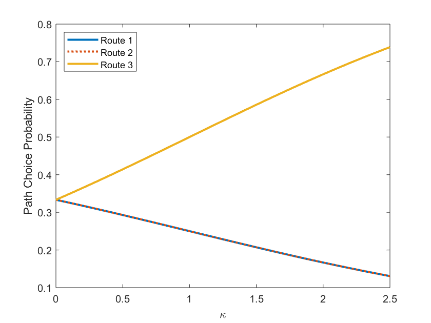
In order to see how our model overcomes the overlapping problem, we study a concrete case. Let us reintroduce the network in Figure 2 where the set of paths is given by with , , and . For this example, let and assume , , and .
As we have previously discussed for this network structure, paths and overlap, sharing the common edge . Under this parameterization of instantaneous utility, coupled with , it follows that , and, consequently, the logit choice rule (14) assigns one third of flow to each path. In other words, with , we get . However, since paths and are identical in utility, the assignment and is a more appropriate allocation.
However, as , the logit model with choice aversion predicts a flow allocation approaching . To understand this, we look at the probability ratio between paths , , and :
| (16) |
From the previous expression, it follows that the value of will affect the ratios and , but not . In particular, Eq. (16) shows that the ratios and are decreasing in . In other words, as the degree of choice aversion increases, the probabilities and decrease while the probability associated to increases.
Now assume that a new edge is added at node which connects to destination node . This implies that the new set of paths is . In terms of Eq. (16), adding implies that:
This latter expression makes explicit the fact that changes in will change the probability ratio between different paths, i.e., IIA does not hold.
3.1. Choice aversion compared to the Adaptive PSL model
What the analysis just laid out shows—which applies to the general case of directed networks—is that from the vantage point of path selection, choice aversion is a robust way to derive path choice probabilities, even in the case of overlapping of different routes. This robustness feature makes our approach similar to the class of PSL models, which is widely used in applied work (e.g. Duncan et al. 2020).
In this section we compare our approach with the APSL model, a state-of-the-art extension of the class of PSL models introduced by Duncan et al. 2020.1414 14 For ease of exposition, we provide the details of the APSL and other PSL models in Appendix A. Figure 4 displays a network topology similar to one featured in Fosgerau et al. 2013. We test the performance of the choice aversion model on this network in calculating path choice probabilities. We assume that this is a directed acyclical graph, where the set of paths is given by with , , , and . Similar to the previous section, let for each edge .
This graph represents a more complex uncongested network topology where the cost of all routes are equal. Thus, the only difference in routes 1 through 4 are the choice sets at each node along the path. The MNL model (equivalent to in the choice aversion model) predicts equal path choice probabilities, i.e., for .
Figure 5(A) shows choice probabilities as increases from 0 to 10. As the choice aversion penalization grows larger, approaches 1, since it is the only route with no alternatives for the user to decide between once the user travels beyond node 1. On the other hand, while and have equivalent choice aversion terms, has the advantage of lacking an additional downstream choice in comparison, allowing for until the choice aversion parameter grows so large that the respective route choice probabilities converge and approach zero.


The prediction in Figure 5(A) differs from route choice probabilities generated by the RL in Fosgerau et al. 2013 and the APSL model proposed by Duncan et al. 2020. This latter model is shown in Figure 5(B). In the Adaptive PSL model, the overlapping path correction is based on correlation of routes through link-path incidence rather than a penalization for size of choice sets along the path. As a result, we see that for the APSL model, for all values of , not as in the choice aversion model.
In other words, the APSL model assigns equal probability to paths 1 and 3 because they share equal edge costs and degrees of overlap with other paths, even as the sequence of costs differs. On the other hand, the choice aversion model assigns equal flow to paths 1 and 2 because they are equal in cost and number of outgoing links at path nodes, where we note that one outgoing link results in a choice aversion penalization of zero.1515 15 We thank an anonymous referee by suggesting this paragraph.
We remark that the behavioral nature of the choice aversion model allows for a different type of correction than APSL model. The choice aversion and the APSL model work in a similar way in the sense of overcoming the overlapping path problem. However, the choice aversion model has a simple and clear behavioral interpretation. This feature sets the choice aversion model apart from other APSL and other PSL models both in terms of interpretation and performance.1616 16 We note that for paths crossing the same nodes, the IIA property holds. To see this, consider paths and , crossing exactly the same nodes. Thus in this case and .
3.2. Fosgerau et al. 2013’s RL and the overlapping path problem
The paper by Fosgerau et al. 2013 proposes a link additive correction attribute called Link Size (LS). The LS correction is similar in spirit to PSL models. However, instead of correcting for the number of paths sharing a given link, the LS correction considers the expected link flow as a proxy for the amount of overlap between paths. Our choice aversion correction is similar to the LS approach in the sense that is link additive, but the mechanism behind the correction of the overlapping paths problem is quite different. Our correction penalizes choice sets while LS penalizes common links. In other words, we focus at the node level while Fosgerau et al. 2013 focus at the link level. Thus, both approaches can be seen as alternatives to each other.
In addition, we mention that our approach differs from Fosgerau et al. 2013 in two important aspects. First, we show that our approach can generate violations of regularity. Second, we show how our model can be useful to characterize changes on welfare when the network is modified. We discuss these two topics in §4 and 5, respectively, and we provide an empirical comparison of these models in §6.
3.3. Mai et al. 2015’s NRL model
The paper by Mai et al. 2015 introduces a Nested Recursive Logit (NRL) model to overcome the overlapping paths problem. Using an approach similar to the Nested Logit (McFadden 1978b), their model allows for path utilities to be correlated where the links can have different scale parameters.
Formally, Mai et al. 2015 extend the RL model in Fosgerau et al. 2013, by allowing the scale parameter of the Gumbel-distributed random variables to be link-specific (in contrast with our Assumption 1). To see how their approach works, consider a link and a node where . Let be an link-specific parameter. Accordingly, the continuation value associated to node is defined as:
| (17) |
From (17) it follows that the link-specific scale parameter affects the continuation values. Based on expression (17), Mai et al. 2015 show that the IIA property can be relaxed using different scale parameters. More importantly, they show how by allowing correlation between path utilities, the NRL generates more realistic path choice probabilities.
Our approach shares the recursive structure of the NRL. However, both models differ in a few key aspects. First, the choice aversion term modifies the level of the associated continuation value, while the link-specific parameter modifies the shape of it. Second, as we discussed above, the inclusion of the choice aversion term allows us to relax the IIA condition. Mai et al. 2015 relax the IIA assumption by allowing correlation across stochastic terms at each node and through the scale parameters . Thus, choice aversion exploits the topology of the network to relax IIA, while the NRL exploits the correlation between the random variables at each node. Third, as we shall see in §4, our approach allows for the failure of the regularity property in the path choice probabilities. This pattern is not captured by the NRL model. A final difference is the fact that our approach allows us to characterize how modifications to the network can be welfare-improving or not. In §5, we discuss this type of exercise.
It is worth remarking that Mai et al. 2015 model the parameter as a function of . Thus, they are able to capture the effect of in the edge and choice probabilities. This latter fact can be seen as an alternative way of capturing the notion of choice aversion. However, there are some key differences between their approach and our choice aversion model.
In order to visualize the differences between the NRL and choice aversion models, we compare path predictions using the example network shown in Figure 6, which was first introduced in Mai et al. 2015.
Figure 6 has five nodes {A, B, C, D, E} and 10 links between the source node A and sink node D. There are six paths from A to D: , , , , , and . We denote these paths by , , , , , and , respectively. Following Mai et al. 2015, link is not considered in the example routes, but its existence affects the continuation values for overlapping paths in the NRL model. Naturally, in the choice aversion model, link is included as an option in the choice set at node .
Following Mai et al. 2015, we use the parameterization and . In addition, we model and as follows:
| (18) |
where refers to the number of outgoing links. Intuitively, captures how the number of outgoing links affects the magnitude of . Given that , we can see from (18) that . Mai et al. 2015 also provide further empirical evidence that . Thus, in order to compare our approach with theirs, we set .
| Route | Route Choice Probabilities | ||
|---|---|---|---|
| Nested RL | Choice Aversion | CA | |
| (, ) | (, ) | () | |
| =() | 0.5541 | 0.4227 | 0.4775 |
| =() | 0.0750 | 0.1555 | 0.1757 |
| =() | 0.0110 | 0.0572 | 0.0323 |
| =() | 0.0567 | 0.0679 | 0.0323 |
| =() | 0.1037 | 0.1120 | 0.1065 |
| =() | 0.1938 | 0.1847 | 0.1757 |
Table 1 displays the differences in choice probabilities predicted by NRL and choice aversion models for the network in Figure 6. For the choice aversion model, we also include a baseline parameterization where for all nodes . Here, we see the difference in predictions between the choice aversion model, which penalizes large choice sets directly, and the NRL model, where more options indirectly adjust the scaling of error terms. In other words, we incorporate the effect of a large choice set in a linear way, while Mai et al. 2015’s approach is nonlinear.
In terms of path choices, the NRL predicts a higher choice probability for routes and relative to the choice aversion model. The reason for this comes from the fact that from a behavioral standpoint, when , the NRL model predicts that the role of the random shocks in user utilities is smaller. In other words, as the magnitude of increases, users’ choice of paths becomes more precise. This effect is particularly important for paths with a large degree of overlapping. In contrast, the choice aversion model predicts lower likelihoods of selecting the least costly routes as choice sets grow larger, which is aligned with the idea that in larger sets of options, the cost of thinking associated to choice aversion increases (Ortoleva 2013 and Fudenberg and Strzalecki 2015).
Finally, we close this section noticing that, given the recursive nature of the choice aversion problem, we can combine our approach with the NRL. To see this note that Eq. (17) can be rewritten as:
Studying the properties of combining these two models is left for future research.
3.4. Mai 2016 versus choice aversion
Mai 2016 proposes a way to estimate a recursive route choice model, which generalizes other existing recursive models in the literature. In particular, this approach can incorporate Multivariate Extreme Value models at each node, which allows him to accommodate general patterns of substitution between different paths. However, Mai 2016 does not consider the problem treated in this paper. In particular, his model can generate neither a failure of regularity nor Braess’s-like phenomena. Furthermore, and similar to Fosgerau et al. 2013 and Mai et al. 2015, the model in Mai 2016 predicts that adding links (or paths) to the network always increases users’ welfare.
4. Choice aversion and the failure of regularity
In the standard MNL (i.e., for all ), adding an additional alternative to the choice set cannot increase the probability that an existing action is selected (and vice versa). This is known as the regularity property in Random Utility models (Luce and Suppes 1965).
Formally, in the context of a route choice, the regularity property states that, given the set of routes and with , we will have:
| (19) |
Intuitively, condition (19) establishes that removing a path from a set should (weakly) increase the choice probability of the remaining paths. Alternatively, adding new paths to the choice set should (weakly) decrease the choice probability of the existing paths in .
In this section, we show that there exists a critical value of , which allows us to understand how varying the network can generate violations of regularity. In order to gain some intuition, we discuss a simple network that allows us to show how regularity may break down. In particular, we study another nested network structure considered in Mai et al. 2015. Figure 7 is a simplified version of Figure 6, such that links and are no longer present. There are still six possible paths from A to D: , , , , , and . Again, we denote these paths by , , , , , and , respectively.
Tables 2 and 3 display route choice probabilities when links , , , and are removed from the nested network in Figure 7. Table 2 shows the results when choice parameters are homogeneous (i.e., ), and Table 3 shows the results when , all else held equal.
| Route | Choice Pr. | Route Choice Probabilities when Edge is Removed | |||
|---|---|---|---|---|---|
| = () | 0.4485 | - | 0.6174 (38%) | 0.4185 (-7%) | 0.4429 (-1%) |
| = () | 0.1650 | 0.3726 (126%) | - | 0.1539 (-7%) | 0.1629 (-1%) |
| = () | 0.0607 | 0.1371 (126%) | 0.0836 (38%) | 0.0566 (-7%) | 0.0599 (-1%) |
| = () | 0.0607 | 0.0914 (51%) | 0.0557 (-8%) | - | 0.0899 (48%) |
| = () | 0.1001 | 0.1506 (51%) | 0.0918 (-8%) | 0.1401 (40%) | - |
| = () | 0.1650 | 0.2484 (51%) | 0.1514 (-8%) | 0.2309 (40%) | 0.2444 (48%) |
| Route | Choice Pr. | Route Choice Probabilities when Edge is Removed | |||
|---|---|---|---|---|---|
| = () | 0.5730 | - | 0.7712 (35%) | 0.5138 (-10%) | 0.5317 (-7%) |
| = () | 0.2108 | 0.5535 (163%) | - | 0.1890 (-10%) | 0.1956 (-7%) |
| = () | 0.0775 | 0.2036 (163%) | 0.1044 (35%) | 0.0695 (-10%) | 0.0720 (-7%) |
| = () | 0.0258 | 0.0453 (75%) | 0.0232 (-10%) | - | 0.0540 (109%) |
| = () | 0.0426 | 0.0746 (75%) | 0.0382 (-10%) | 0.0860 (102%) | - |
| = () | 0.0703 | 0.1230 (75%) | 0.0630 (-10%) | 0.1417 (102%) | 0.1467 (109%) |
From Table 2, we note that when link is removed, the choice probabilities of remaining paths {, …, } increase. Note that the probabilities of paths and increase in the same proportion (126%). Similarly, the probabilities of paths , , and also increase in the same proportion (51%). Each increase is even more pronounced in Table 3 where . However, in both tables, the increase is not proportional across paths crossing different nodes. This feature comes from the IIA property, which holds within nodes (nests) but not across them.
Now, consider the case of removing edge . In Table 2, the probabilities of paths and increase proportionally (38%). However, the probability of paths , , and actually decrease. This counterintuitive result is a consequence of the fact that removing edge not only reduces the number of available paths but also decreases the cost associated to paths and . In other words, this effect can be decomposed into two parts. First, the IIA property implies that the probabilities of , , , , and will increase upon removing edge . The second force behind this counterintuitive result is that removing edge reduces the choice set when taking paths and . For a choice averse user, this latter effect implies that reduces to , which makes paths and relatively more attractive than , , and , such that the probabilities of , , and decrease. When this second effect dominates, we will observe the failure of regularity associated with removing edge .
It may be tempting to think that the effect in path choices described above may be driven by the assumption that is homogeneous. However, Table 3 shows that a similar pattern occurs when we consider and . In this case, the failure of regularity is even more pronounced through relatively larger changes to remaining path probabilities.
We formalize the previous intuition in Proposition 1 below. In doing so, recall that is the set of paths passing through node . Similarly, the set of paths not passing through node is defined as . In addition, define as the set of paths passing through node after removing edge at node . Finally, let and .
Proposition 1.
The probability of choosing a path decreases after removing an edge if
| (20) |
Some remarks are in order. First, Proposition 1 provides a simple condition to know when removing an edge at node will decrease the probability of paths not crossing node . Condition (20) captures the fact that removing an edge at node will not only modify the set of available paths but also the choice aversion cost. Concretely, condition (20) establishes a lower bound on the parameter in terms of the path choice probabilities and and the magnitude of and . To the best of our knowledge, this result is new to the literature on recursive discrete choice models in transportation networks.
Second, we note that, from a practical point of view, Proposition 1 is useful because it allows us to understand how modifying the structure of the network can have different effects in terms of flow prediction (choice probability). In particular, (20) establishes a simple condition to understand the choice behavior as a function of the parameter , which is node-specific. Thus, when designing interventions in transportation networks, Proposition 1 helps us to understand how users’ behavior will react to such interventions.
Third, Proposition 1 predicts that removing edge can decrease the probability of paths passing through nodes different from . We have identified this phenomenon as a failure of regularity in the sense of Luce and Suppes 1965. However, behind this result is the factor that reducing the cardinality of reduces the penalization associated with choice aversion. This reduction effect can dominate, making paths crossing node more attractive than before. As a consequence, the choice probabilities of paths crossing node should increase while the choice probability of paths not crossing node should decrease.
In the context of rational inattention, Matějka and McKay 2015 have shown that regularity may fail in the logit model. Our result is different in two aspects. First, we study a RL model with choice aversion in the context of transportation networks. Second, our result highlights the role of choice aversion by providing a specific condition on . Matějka and McKay 2015 use the idea of information acquisition in order to derive their result.1717 17 We note that Matějka and McKay 2015’s analysis has been extended to the general class of additive random utility models by Fosgerau et al. 2020.
Finally, we mention that a particular case of Proposition 1 is when for all .
In order to see how Proposition 1 applies in the concrete case of the network in Figure 7, Table 4 summarizes the information after removing edges , , , and , respectively. The main message from this table is the simplicity in checking Proposition 1.
| Edge Removed | Condition |
|---|---|
5. Welfare Analysis and Braess’s Paradox
In previous sections we have shown how the recursive choice aversion model corrects the problem of predicting routing behavior when there are overlapping paths. Similarly, we have shown how this model may generate violations of regularity when some edge of the network is removed.
In this section, we show how choice aversion can capture changes to users’ welfare when the network topology is modified. Formally, we show that under the presence of choice aversion, adding edges to the network can decrease users’ welfare. In particular, we show how a type of Braess’s paradox (Braess 1968 and Braess et al. 2005) can emerge even in the case of uncongested networks.
5.1. Welfare
Following McFadden 1981, we define the users’ welfare as follows:
| (21) |
where the last equality follows from Assumption 1 and . Notice that this definition exploits the equivalence in Eq. (11) and makes explicit the dependence of users’ welfare on the choice aversion parameters . We say that iff for all
Following the literature on discrete choice models, expression (21) can be interpreted as the inclusive value of paths in , which is equivalent to say that measures the inclusive value of the source node . In particular, represents the expected utility faced by the network users.
We now establish some properties of .
Proposition 2.
The function satisfies the following properties:
- a)
Let . Then .
- b)
Consider a node and an edge . Then
- c)
Consider a node . Then
Part a) of Prop. 2 shows an intuitive result: users’ welfare decreases when the choice aversion parameter vector increases. Part b) establishes that an increase in the utility of an edge , , subsequently increases users’ welfare by the amount of flow received by edge . Finally, part c) of Prop. 2 allows us to predict precisely how much users’ welfare decreases when the choice aversion parameter increases. Quantitatively, decreases by the sum of the path choice probabilities of all paths passing through node , multiplied by the natural log of the size of the choice set at node , .
Next, we show how changes in response to adding or deleting edges to the network To that end, we connect changes on with changes on when the network is modified. Formally, we have the following:
Proposition 3.
Fix a node . Suppose that a new link is added to node . Then increases if and only if the following condition holds:
| (22) |
It is worth stressing three implications of this result. First, Proposition 3 underscores the way in which local effects—namely, the addition of alternatives at the node level—propagate throughout the transportation network and unlock aggregate welfare effects. Second, it connects the axiomatic characterization of stochastic choice in dynamic settings from Fudenberg and Strzalecki 2015 with transportation networks. In particular, our Proposition 3 extends their Proposition 3 to the case of transportation networks and graph-related settings. Finally, and most notably, it shows that Braess’s network paradox may equivalently stem from choice aversion with no allusion to congestion whatsoever.
From an economic standpoint, Proposition 3 characterizes how adding an edge to the network is welfare-improving as a function of the value of . In particular, after the new edge has been added, Eq. (22) can be easily checked to know whether increases or decreases. Subsequently, the choice aversion model predicts that there exists a range of values for the choice aversion parameter where the addition of new edges can lead to a decrease in welfare, even if the utility of newly created routes is higher than existing routes. Thus, we can predict the emergence of Braess’s paradox-like phenomena in the case of uncongested transportation networks through Proposition 3. §5.2 discusses this result in detail.
We note that from an empirical point of view, Eq. (22) can be estimated providing a simple test to understand when modifications to the network are welfare-improving or not.
Finally, we point out that, in Appendix C, we carry out a welfare analysis comparing our approach with several PSL models, including the APSL.
5.2. Braess’s paradox as the outcome of choice aversion
Proposition 3 provides a simple condition that characterizes the way in which an improvement at the node level may increase consumer surplus. This result can be connected to Braess’s paradox, which states that adding free routes into a transportation network makes every decision maker worse off (Braess 1968; Braess et al. 2005). The connection we establish is that we may generate this phenomenon as a consequence of choice aversion in a general directed network.
In order to see how our result is related to Braess’s paradox, consider the special directed networks given in Figures 8(A) and 8(B). Figure 8(A) shows a parallel serial network with paths and . The set of paths therefore is given by , and welfare described by
Now assume that the network in Figure 8(A) is modified by means of adding a new edge starting at node and ending at node , as Figure 8(B) shows. Now the new set of paths is given by , where and are defined as before and . Users’ surplus for this modified network is given by:
Proposition 3 allows us to characterize the effects of adding edge into the original network. In particular, iff
In other words, moving from network 8(A) to 8(B) improves users’ welfare if and only if the probability of choosing is strictly greater than , which is automatically satisfied when . To state this condition in terms of , we assume and with . Given this parameterization, it is easy to see that and .
Then if and only if
which can be rewritten as
It is easy to see that for we have if and only if .1818 18 Note that for we have .
As we mentioned in §2, the case of corresponds to a situation where users only want to add alternatives that are sufficiently better that the existing ones. In this case, network users want to add edge whenever . In particular, for values of , improving the network can make all users worse off. Thereby, under choice aversion, we can obtain the very same type of paradox described by Braess 1968 and Braess et al. 2005. However, while this paradox is usually obtained as a consequence of network users’ selfish behavior in a congestion game, we derive it as a consequence of choice aversion, which provides a different perspective to the problem of network design.
6. Empirical Analysis
In this section, we move beyond calibration of the choice aversion model and econometrically estimate the choice aversion parameter . Using observed data on paths taken across a given real-world network structure, we can employ maximum likelihood estimation (MLE) procedures to estimate . Previous literature on RL models in transportation networks use MLE routines to analyze the performance and strength of existing models (Fosgerau et al. 2013, Mai et al. 2015, Zimmermann et al. 2017a, Zimmermann and Frejinger 2020). Following this precedence, we exploit a similar approach, incorporating the choice aversion penalization in the utility function of the network user to estimate the value of alongside other network attributes.1919 19 The MATLAB code used for the empirical exercises in this section are available online or upon request, along with all other code used for this paper.
Through the following empirical analysis, we demonstrate a set of key strengths of the choice aversion model. First, we show that the obtained estimates for the choice aversion parameter are similar to calibrations given for the simulations on example networks, thus validating the legitimacy of the model and previous inferences from such exercises. Second, we show that the choice aversion model exhibits a similar performance to other RL models in terms of mechanical path prediction on transportation flows. Finally, because of the parsimonious nature of the choice aversion penalty, we show that the model is less computationally demanding, performing at much faster speeds than other corrective additions to the RL model.
6.1. Illustrative Tutorial Example in Zimmermann et al. 2017b
We first test the choice aversion model on an illustrative example network used as a tutorial for estimation of the RL model (Zimmermann et al. 2017b) and depicted in Figure 9. This network contains 17 nodes and 29 edges, with 2 origin-destination source-sink pairs (1 to 17 and 2 to 17). There are 100 synthetic path observations over this network generated by a linear utility specification with three attributes: link length, existence of a traffic signal, and a link constant.
For this network, we estimate the traditional RL model, a RL that incorporates the choice aversion attribute, and a RL model with the Link Size attribute introduced by Fosgerau et al. 2013 and discussed in Section 3.2. For the straightforward RL specification, we follow the original authors and estimate coefficients for link length, traffic signal, and a link constant. In addition to this specification, we incorporate the choice aversion term to estimate , the choice aversion parameter.2020 20 For simplicity, we assume that is homogeneous across nodes in the network. We anticipate future empirical work to relax and test this condition. For the sake of comparison, we also incorporate the Link Size attribute, which allows users to account for expected flows based on link attributes. We test these specifications both separately and together, as well as allowing for an interaction term between choice aversion and Link Size. These specifications are detailed formally in Eq. (23).2121 21 Note that for is equivalent to for . We have made this modification for the empirical section of the paper to be consistent with testing our hypothesis alongside other attributes in the RL framework.
| (23) |
Table 5 displays the estimates obtained through the MLE routine conducted across the network for each specification previously mentioned. As may be expected for this tutorial data, the coefficients for link length and traffic signal are the only attributes where significant estimates are consistently observed across specifications.
| RL | RL-CA | RL-LS | CA & LS | CA LS | |
| -2.323 | -2.284 | -2.269 | -2.023 | -2.392 | |
| Std. Error | (0.304) | (0.301) | (0.475) | (0.362) | (0.564) |
| t-test | -7.642 | -7.586 | -5.651 | -5.582 | -4.243 |
| -0.337 | -0.253 | -0.297 | 0.235 | -0.275 | |
| Std. Error | (0.105) | (0.120) | (0.115) | (0.418) | (0.123) |
| t-test | -3.225 | -2.103 | -2.575 | 0.562 | -2.232 |
| 0.061 | 0.196 | 0.355 | 0.082 | 0.202 | |
| Std. Error | (0.231) | (0.224) | (0.373) | (0.253) | (0.401) |
| t-test | 0.264 | 0.875 | 0.951 | 0.325 | 0.505 |
| — | -0.539 | — | -0.559 | -0.261 | |
| Std. Error | - | (0.364) | - | (0.374) | (0.497) |
| t-test | -1.481 | -1.495 | -0.525 | ||
| — | — | -0.628 | 0.455 | 0.499 | |
| Std. Error | - | - | (0.695) | (0.381) | (1.025) |
| t-test | -0.904 | 1.194 | 0.487 | ||
| — | — | — | — | -1.119 | |
| Std. Error | - | - | - | - | (1.298) |
| t-test | -0.862 | ||||
| N | 100 | 100 | 100 | 100 | 100 |
| LL | 2.374 | 2.361 | 2.370 | 2.354 | 2.357 |
| Elapsed Time (sec) | 0.576 | 0.628 | 2.441 | 3.243 | 5.350 |
In contrast, it does not appear that either choice aversion or Link Size are important attributes to network users under this construction, although they appear to cut into the explanatory power of the preceding variables in some specifications. Given this, we note that the estimated choice aversion parameter is consistently negative, while the Link Size attribute ranges between positive and negative values. Additionally, we note that incorporating the Link Size attribute in the specification dramatically decreases the speed of the MLE routine.
6.2. Borlänge Traffic Network
Next, we test our model on GPS vehicle data observed in the city of Borlänge, Sweden. This traffic data set is well known and has been previously used to test RL models in Fosgerau et al. 2013 and Mai et al. 2015. Over a span of two years, a sample of 1,832 trips (using a minimum of five links) were observed across a network with 3,077 nodes and 7,459 links (21,452 link pairs). This network includes 466 unique destinations and 1,420 different origin-destination pairs. Most importantly, network users have over 37,000 link choices, making this real-world network a suitable application for testing the choice aversion model.
Using this data, we proceed with the standard RL model with and without choice aversion and the Link Size attribute as in Section 6.1. The specifications used for the MLE routines in this section are identical to those shown by Eq. (23), except there is no traffic signal attribute to this data.2222 22 Fosgerau et al. 2013 and Mai et al. 2015 include additional network attributes regarding turn angles in their empirical analysis. We omit these from our analysis for the sake of simplicity and clarity.
| RL | RL-CA | RL-LS | CA & LS | CA LS | |
| -3.901 | -3.738 | -3.930 | -3.582 | -3.525 | |
| Std. Error | (-0.127) | (0.124) | (0.136) | (0.145) | (0.141) |
| t-test | -30.828 | -30.062 | -28.918 | -24.725 | -25.031 |
| -1.155 | -0.936 | -1.251 | -0.567 | -0.744 | |
| Std. Error | (0.015) | (0.049) | (0.018) | (0.040) | (0.056) |
| t-test | -77.294 | -18.923 | -69.314 | -14.180 | -13.380 |
| — | -0.199 | — | -0.624 | -0.481 | |
| Std. Error | - | (0.042) | - | (0.035) | (0.048) |
| t-test | -4.715 | -17.279 | -10.060 | ||
| — | — | -0.557 | -0.475 | -0.031 | |
| Std. Error | - | - | (0.018) | (0.017) | (0.086) |
| t-test | -31.124 | -27.470 | -0.365 | ||
| — | — | — | — | -0.419 | |
| Std. Error | - | - | - | - | (0.078) |
| t-test | -5.395 | ||||
| N | 1832 | 1832 | 1832 | 1832 | 1832 |
| LL | 5.648 | 5.627 | 4.874 | 4.978 | 4.957 |
| Elapsed Time (sec) | 49.413 | 85.832 | 3738.069 | 5130.600 | 5357.333 |
Table 6 displays the results for each specification on the Borlänge network. For this data, the estimated choice aversion parameter is significant and negative, ranging between and . This result provides evidence that network users are indeed choice averse and to a degree that is consistent with calibrations presented in Sections 2-5. We note that and are similar in range of values and are both significant across specifications, demonstrating that choice aversion has the capability of providing predictive power on transportation networks like Link Size and other additions to the RL model.
We note that for a complex network such as Borlänge, choice aversion does not even double the speed of the MLE routine, while incorporating the Link Size attribute may cause the time required for convergence to increase exponentially. While we also observed a decrease in speed of Link Size for the tutorial data, the decline observed with this data is much sharper moving from the RL to the RL-LS (by over a factor of 75). From an applied perspective, the combination of speed, tractability, and economic interpretation of the choice aversion model should prove attractive when compared to other RL models.
The last column in Table 6 displays a coefficient for Link Size that is not significant, while also displaying a negative and significant estimate for the interaction term . It is intuitive that expected flows and choice aversion are in tandem with one another in terms of affecting individual routing decisions. We interpret this result as an indicator that there is more to understand about the role of choice aversion among users in complex, congested networks. We leave this discussion to be explored more deeply in future empirical and experimental work.
Finally, we note that using the RL-LS rather than the RL-CA results in a larger improvement of the log-likelihood compared to the RL, suggesting that the RL-LS may outperform the RL-CA in this regard. In Appendix D, we conduct an out-of-sample validation analysis to compare performance across RL models. The main conclusion of this exercise is that the RL-LS and RL-CA exhibit similar out-of-sample performance.
7. Final Remarks
The recursive choice model with choice aversion is a highly tractable extension of the standard RL model that can be used to predict reasonable route choice probabilities and provide welfare interpretations in transportation networks. Upon testing our approach against existing PSL models, our model exhibits the power to provide reasonable corrections and predictions with the benefit of a microfoundation in choice overload.
In addition, we explore how the choice aversion model allows for a break in the regularity condition typically preserved by path choice probabilities in logit models and extensions. In doing so, we show that, conditional on the degree of choice aversion, removing edges in the network can lead to a decrease in choice probability of certain existing paths.
We also simulate the welfare implications of the choice aversion model and find a novel prediction: even in uncongested networks, a decrease in welfare akin to Braess’s paradox can arise when costless edges are added. Here, we also provide a simple characterization for welfare changes conditional on choice aversion which is testable in empirical settings.
Furthermore, we estimate our model providing evidence that users in transportation networks suffer from choice aversion. An important extension of this work is to consider the role of choice aversion in the context of congested traffic networks and the respective modeling approach. One way to study this question is to extend the model in Baillon and Cominetti 2008 by introducing choice aversion in their recursive approach.
Finally, we remark that there is much work to be done regarding the empirical support of choice aversion in transportation networks. We anticipate there is more to understand regarding the role of node-specific (or nest-specific) choice aversion within complex real-world environments. Similarly, we point out that our empirical analysis assumes a homogeneous choice aversion parameter. However, in real-life transportation networks, it is reasonable to assume that depends on users’ characteristics. We leave for future research the econometric analysis of this type of model.
Future work regarding experiments on behavior of participants in transportation networks would help establish a better understanding of the significance of choice overload in making routing choices.
References
- Acemoglu et al. (2018) Acemoglu, D., Makhdoumi, A., Malekian, A., and Ozdaglar, A. (2018). Informational braess’ paradox: The effect of information on traffic congestion. Operations Research, 66(4):893–917.
- Baillon and Cominetti (2008) Baillon, J. B. and Cominetti, R. (2008). Markovian traffic equilibrium. Math Program. Ser. B, 111:33–56.
- Ben-Akiva and Bierlarie (1999) Ben-Akiva, M. and Bierlarie, M. (1999). Discrete choice methods and their applications to short term travel decisions. Handbook of transportation Science, pages 5–34.
- Ben-Akiva and Lerman (1985) Ben-Akiva, M. and Lerman, S. (1985). Discrete Choice Analysis: Theory and Application to Travel Demand. MIT Press, Cambridge, 1 edition.
- Ben-Akiva and Ramming (1998) Ben-Akiva, M. and Ramming, M. S. (1998). Lecture notes: discrete choice models of traveler behavior in networks. Prepared for Advanced Methods for Planning and Management of Transportation Networks .
- Braess (1968) Braess, D. (1968). Uber ein paradoxon aus der verkehrsplanung. Unternehmensforschung, 12(1):258–268.
- Braess et al. (2005) Braess, D., Nagurney, A., and Wakolbinger, T. (2005). On a paradox of traffic planning. Transportation Science, 39(4):446–450.
- Chu (1989) Chu, C. (1989). A paired combinatorial logit model for travel demand analysis. Transport Policy, Management and Technology Towards 2001:Selected Proceedings of the Fifth World Conference on Transport Research, 4:295–309.
- Duncan et al. (2020) Duncan, L. C., Watling, D. P., Connors, R. D., Rasmussen, T. K., and Nielsen, O. A. (2020). Path size logit route choice models: Issues with current models, a new internally consistent approach, and parameter estimation on a large-scale network with gps data. Transportation Research Part B: Methodological, 135:1 – 40.
- Fosgerau et al. (2013) Fosgerau, M., Frejinger, E., and Karlstrom, A. (2013). A link based network route choice model with unrestricted choice set. Transportation Research Part B: Methodological, 56:70–80.
- Fosgerau and Jiang (2019) Fosgerau, M. and Jiang, G. (2019). Travel time variability and rational inattention. Transportation Research Part B: Methodological, 120:1 – 14.
- Fosgerau et al. (2020) Fosgerau, M., Melo, E., de Palma, A., and Shum, M. (2020). Discrete choice and rational inattention: A general equivalence result. International Economic Review, 61(4):1569–1589.
- Frejinger and Bierlarie (2007) Frejinger, E. and Bierlarie, M. (2007). Capturing correlation with subnetworks in route choice models. Transportation Research Part B, pages 363–378.
- Fudenberg and Strzalecki (2015) Fudenberg, D. and Strzalecki, T. (2015). Dynamic logit with choice aversion. Econometrica, 83(2):651–691.
- Gilbert et al. (2014) Gilbert, F., Marcotte, P., and Savard, G. (2014). Logit network pricing. Computers & Operations Research, 41.
- Jiang et al. (2020) Jiang, G., Fosgerau, M., and Lo, H. K. (2020). Route choice, travel time variability, and rational inattention. Transportation Research Part B: Methodological, 132:188 – 207. 23rd International Symposium on Transportation and Traffic Theory (ISTTT 23).
- Koppelman and Wen (2000) Koppelman, F. S. and Wen, C.-H. (2000). The paired combinatorial logit model: properties, estimation and application. Transportation Research Part B: Methodological, 34(2):75 – 89.
- Kreps (1979) Kreps, D. (1979). A representation theorem for “preference for flexibility”. Econometrica, 47(3):565–577.
- Luce (1959) Luce, D. R. (1959). Individual Choice Behavior: A Theoretical Analysis (Dover Books on Mathematics). Dover Publications, 1 edition.
- Luce and Suppes (1965) Luce, D. R. and Suppes, P. (1965). Preference, utility, and subjective probability. New York: John Wiley & Sons, 1 edition.
- Mai (2016) Mai, T. (2016). A method of integrating correlation structures for a generalized recursive route choice model. Transportation Research Part B: Methodological, 93:146–161.
- Mai et al. (2015) Mai, T., Fosgerau, M., and Frejinger, E. (2015). A nested recursive logit model for route choice analysis. Transportation Research Part B: Methodological, 75:100 – 112.
- Matějka and McKay (2015) Matějka, F. and McKay, A. (2015). Rational inattention to discrete choices: A new foundation for the multinomial logit model. American Economic Review, 105(1):272–98.
- McFadden (1974) McFadden, D. (1974). Conditional logit analysis of qualitative choice behavior. Frontiers in Econometrics, pages 105–142.
- McFadden (1978a) McFadden, D. (1978a). Behavioural travel modelling, chapter 13: Quantitive methods for analyzing travel behaviour of individuals: some recent developments, pages 279–318. Croom Helm London.
- McFadden (1978b) McFadden, D. (1978b). Modeling the choice of residential location. in A. Karlqvis, A., Lundqvist, L., Snickars, L., Weibull, J. (eds.), Spatial Intearction Theory and Planning Models (North Holland, Amsterdam), pages 531–551.
- McFadden (1981) McFadden, D. (1981). Structural Analysis of Discrete Data with Econometric Applications, chapter Econometric Models of Probabilistic Choice, pages 198–272. Cambridge: MIT.
- Ortoleva (2013) Ortoleva, P. (2013). The price of flexibility: Towards a theory of thinking aversion. Journal of Economic Theory, 148(3):903 – 934.
- (29) Ramming, M. S. Network knowledge and route choice. Ph.D. Thesis, Massachusetts Institute of Technology.
- Scheibehenne et al. (2010) Scheibehenne, B., Greifeneder, R., and Todd, P. M. (2010). Can There Ever Be Too Many Options? A Meta-Analytic Review of Choice Overload. Journal of Consumer Research, 37(3):409–425.
- Sheena and Lepper (2000) Sheena, I. and Lepper, M. R. (2000). When choice is demotivating: can one desire too much of a good thing ? Journal of Personality and Social Psychology, 79(6):995–1006.
- Train (2009) Train, K. (2009). Discrete Choice Methods with Simulation. Cambridge University Press, second edition.
- Vosha (1997) Vosha, P. (1997). The cross-nested logit model: application to mode choice in the Tel-Aviv metropolitan area. Transportation Research Record, pages 6–15.
- Vosha and Bekhor (1997) Vosha, P. and Bekhor, S. (1997). The cross-nested logit model: application to mode choice in the Tel-Aviv metropolitan area. Transportation Research Record, pages 6–15.
- Wen and Koppelman (2001) Wen, C.-H. and Koppelman, F. S. (2001). The generalized nested logit model. Transportation Research Part B, 35:627–641.
- Zimmermann and Frejinger (2020) Zimmermann, M. and Frejinger, E. (2020). A tutorial on recursive models for analyzing and predicting path choice behavior. EURO Journal on Transportation and Logistics, 9(2):100004.
- Zimmermann et al. (2017a) Zimmermann, M., Mai, T., and Frejinger, E. (2017a). Bike route choice modeling using gps data without choice sets of paths. Transportation Research Part C: Emerging Technologies, 75:183–196.
- Zimmermann et al. (2017b) Zimmermann, M., Mai, T., and Frejinger, E. (2017b). The recursive logit model tutorial. Cirrelt Seminar, August 2017.
Appendix A Path size logit models
PSL models include correction terms to penalize routes that share links with other routes, so that the deterministic utility of route is where is a correction term for route The probability that a user chooses path is given by:
| (24) |
Following Ben-Akiva and Bierlarie 1999, Path Size Logit (PSL) models adopt the form where is the path size scaling parameter, and is the path size term for route
Let , where is the instantaneous cost of all edges along path and is a cost scaling parameter. A distinct route with no shared links has a path size term equal to resulting in no penalization. Less distinct routes have smaller path size terms and incur greater penalization. The probability that a user chooses route is:
The Path Size Logit (PSL) model was first proposed by Ben-Akiva and Ramming 1998, and states that the PSL path size term for route is defined as follows:
| (25) |
where if edge belongs to path and otherwise.
In Eq. (25), each link in route is penalized (in terms of decreasing the path size term and increasing the cost of the path) according to the number of paths in the choice set that also use that and the significance of the penalization is weighted according to how prominent edge is in route , i.e. the cost of edge in relation to the total cost of path , .
A.1. Generalized Path Size Logit (GPSL)
Ben-Akiva and Bierlarie 1999 formulate an alternative PSL model (PSL’) that attempts to reduce the contributions of excessively expensive routes to the path size terms of more realistic routes in the choice set. The PSL’ model states that the PSL path size term for route is defined as follows:
| (26) |
where if edge is in path and otherwise.
In Eq. (26) the contribution of route to path size terms is weighted according to the ratio of route and the cheapest route in the choice set and hence contributions of high costing routes compared to the cheapest alternative are reduced.
As Ramming describes, however, when a route is completely distinct its path size term is not always equal to 1 which results in an undesired penalization upon the utility of that route. To combat this, Ramming proposes the Generalized Path Size Logit (GPSL) model. The GPSL model states that the GPSL path size term for route is defined as follows:
| (27) |
where if edge is in path and otherwise and . It is easy to see that the GPSL model is equivalent to the PSL model when In Eq. (27) the contribution of route to the path size term of route (the path size contribution factor) is weighted according to the cost ratio between the routes, and hence the contributions of high costing routes to the path size terms of low costing routes is reduced. is the path size contribution scaling parameter to be estimated.
A.2. Adaptive Path Size Logit Model (APSL)
In an attempt to improve on existing PSL models and extensions, Duncan et al. 2020 propose an internally consistent PSL model where all components assess the feasibility of routes according to its relative attractiveness due to travel cost and distinctiveness. Formally, their correction can be defined as follows:
Definition 1.
The APSL choice probabilities, are a solution to the fixed-point problem where:
| (28) | |||||
| (29) | |||||
| (30) |
Despite the fact that there is no closed-form representation of the choice probabilities for the APSL model, the APSL model corrects for many of the internal consistency issues in route cost and distinctiveness that trouble other PSL models, which makes its recent introduction in the literature particularly useful in working to predict route choice probabilities more appropriately.
Appendix B Proofs
B.1. Proof of Proposition 1
First, recall that is the set of paths passing through node , and similarly, the set of paths not passing through node is defined as . We note here that and . Finally, recall that is the set of paths passing through node after removing edge at node . Note that before and after removing an edge the set is the same.
We remark that after the edge at node is removed, the utility of paths in can be expressed as
where . Note that is constant across all paths in . Finally, recall that and .
Without loss of generality, fix a path . Let and be the probability of choosing path before and after removing edge at node , respectively. We want to show under what conditions
we have for any path .
Note that can be written as:
Dividing the numerator and denominator by , we find that:
From the previous expression, it follows that can be expressed as:
Since , it follows that is negative iff
Rearranging this expression, we get
Using the fact that , we get
Noting that , then we conclude:
The following lemma shows that the utility associated to paths passing through node can be decomposed in a simple way.
Lemma 1.
For each node the following holds:
where .
Proof. Let be defined as with , and let be defined as . Then it follows that we can construct the utility associated to all paths of the form as . In particular, we have . Exploiting the recursive structure of the problem, it is easy to see that .
This latter expression implies that
Adding up over all we conclude that:
Previous analysis holds for all node , then the conclusion follows.
B.2. Proof of Proposition 2
a) Consider a path and assume that . By the definition of , let us set . Then it is easy to see that for all . In particular and summing over all we get:
Taking the log in the previous expression, we conclude .
b) By Lemma 1 it is easy to see that
Taking the differential with respect to , we get
Noting that we conclude that:
c) Using the definitions of and , can be written as:
Computing the differential, we find:
Noting that , we conclude that
B.3. Proof of Proposition 3
The proof of this result exploits the recursive structure of the problem. Let denote the set of paths after adding a new link . Accordingly, define . Let and be consumer surplus before and after the addition of , respectively. Note that and .
Adding edge increases consumers’ surplus if and only if the following hold:
Noting that previous conditions boils down to:
| (31) |
By Lemma 1 we can write the following:
Similarly
where denotes the recursive utility (1) after adding edge .
Then Eq. (31) can be written as follows:
| (32) |
Previous expression can be written as:
Then after some algebra we find:
Using the fact that we can conclude that if and only if
Appendix C Welfare exercises using PSL and the choice aversion model
In this appendix we discuss how, in addition to being able to compute changes on welfare using the choice aversion model, we also compute changes in welfare using several PSL models. In particular, for this class of models, the welfare is defined as follows:
| (33) |
where is a parameter vector describing the specific PSL model and represents the adjusted utility after applying the respective correction.
It is worth pointing out that the PSL models are not designed to capture changes on welfare. So, Eq. (33) should be interpreted as an adapted welfare measure. The reason to consider these measures is to compare how traditional PSL models might be used to compute welfare changes with the choice aversion model.
C.1. Braess’s Paradox
As we have seen in Section 5.2, the choice aversion model reveals that welfare decreases can arise naturally even when networks are uncongested through increasing choice set cardinality.2323 23 Note that in the case of uncongested networks, users do not get involved in strategic interaction. In this section of the appendix, we will compare how the choice aversion model handles welfare changes relative to existing PSL models. Let , and consider the parameterization of Figure 8(A) where with and . As we saw in Section 5, this figure depicts the case of a simple parallel serial link network where the set of paths is given by with and .
Figure 8(B) shows the network with edge added to the directed acyclical graph, connecting to . For the purpose of observing Braess’s paradox, we set . The set of paths is given by , where . We calculate the welfare according to (21) for 8(A) and 8(B) and compare the difference.
According to Proposition 3, we can compute the threshold for that determines when adding links is welfare improving.2424 24 For a concise reading, we refer to simply as , since it is clear we are referring to node in this example. In particular, we have that adding a link is welfare-improving when
After some algebra, we can express a relationship between and as follows:
| (34) |
From (34) it is easy to see that when adding an edge is welfare improving when , approximately. Similarly, when , the welfare increases when . In particular, Eq. (34) shows that there is an inverse relationship between and .
Based on this observation, we show how changes when varies for a constant . Figure 10 shows the welfare change for the choice aversion model with as well as the MNL model and other PSL models and extensions mentioned in Section 4.
The choice aversion model where matches this characterization, reflecting a welfare upgrade for and a welfare downgrade when .

In contrast, the MNL model only reflects a nonnegative change in welfare from adding edge , a symptom of a model where additional gains in welfare are realized from any additional route added to the choice set of the agent. From a theoretical standpoint, this feature of the MNL model captures the preference for flexibility in users’ preferences (Kreps 1979).
Interestingly, most PSL models and extensions shown in Figure 10 reflect a welfare change similar to each other: a initial welfare gain which decreases in , ultimately leading to a decrease in welfare.
However, Duncan et al. 2020’s Adaptive PSL model breaks from the welfare change pattern observed by other models. For this model, the difference in welfare is positive and decreasing until , but for , the change in welfare is zero. This is a compelling result which speaks to the strengths of this PSL extension.2525 25 To understand why the APSL differs from traditional PSL models, we note that when , with the equality holding only for . Here, it is reasonable that we would observe an increase in welfare when is added to the network: for an uncongested network, we are adding a cheaper route choice for users, and it is intuitive that this would improve welfare. Indeed, this result is consistent with most models as shown in Figure 10. However, for , where , the APSL model reflects no decrease in welfare. Again, this is intuitive: when , adding costless edge does not provide users with a cheaper route choice. Since the users would incur cheaper costs from choosing routes or , the APSL model considers to be an irrelevant addition to the choice set and thus would not contribute to, nor detract from, welfare.
As we have discussed in great detail already, an important property of the choice aversion model is its microfoundation based in the behavioral concept of choice overload, which provides justification for the penalization term in the utility function as well as the observed outcomes. While there is a similar welfare difference observed among the choice aversion model with and other PSL models and extensions, this microfoundation sets the choice aversion model apart from other models.
It is important to note the contrast in welfare change between and for the choice aversion model. For , Figure 10 clearly shows that there is no value of such that a positive welfare change will be observed. Again, the decrease in welfare stems from a dominating penalization on path utilities by the choice aversion term, amplified by the choice aversion parameter . This contrast is important and draws our attention to how welfare changes as varies for a fixed .


Figure 11(A) shows how the difference in welfare calculated by the choice aversion model responds to an increase in from 0 to 10 for fixed . For each value of displayed, we first see a positive difference in welfare for low values of . As increases, the difference in welfare continues to decrease until the welfare change is negative. In other words, we see that the threshold (i.e., the where the welfare change from adding edge is no longer positive) decreases in . This occurrence stems from the fact that for low values of , the instantaneous cost of each route dominates the choice aversion term in the users’ utility functions. Thus, for low values of , the welfare change is initially positive, but as increases, the choice aversion term is updated with increasing weight until the user’s aversion to choice dominates any increase in utility from an additional route created by .
While the choice aversion model predicts this welfare decrease as a result of its behavioral motivation, other logit models may not provide the same outcome. For example, the APSL model does not show a welfare decrease for any value of as shown by Figure 11(B). Rather, this model seems to predict that the welfare change is nonnegative for all values of and only positive for .2626 26 Despite the difference in behavioral foundation, in the choice aversion model and in most PSL models, including the APSL model, serve a similar purpose of correcting the degree of overlapping between routes sharing common links. However, quantitatively we cannot compare and . While this may be sensible for , we would expect that a model looking to explain decision-making behavior accurately would display a continuous tradeoff between route costs and aversion to increasing choice set cardinality. However, we see that the threshold , where the welfare change is no longer positive, is approximately 1 for all values of featured and most notably for . The APSL model does not seem to be capable of taking into account the tradeoff mentioned above, perhaps as a result of its corrective nature and intentional design. While the APSL model and other PSL models may have a strength in producing more intuitive route choice probabilities, there appears to be a weakness in predicting reasonable welfare changes from a behavioral point of view.
To summarize, while PSL models and extensions are developed to correct the outcome of a standard logit model and provide what may be deemed as more reasonable choice probabilities for a given network topology, what they often lack is the behavioral foundation for any penalties or adjustments in the cost function of the network user, which would justify the outcomes they provide. Their designs also limit their capability to model changes in welfare with respect to internal parameters. This is not to say that the existing PSL models are inferior; indeed, these models are powerful and useful in various applications at providing reasonable predictions in network flow allocations.2727 27 For instance, Duncan et al. 2020 analyze an example similar to Figure 2. Their conclusions, while being quantitatively different, agree with the predictions made by the choice aversion model. We simply wish to speak to the strengths of the choice aversion model in the context of applications in transportation networks where choice overload is a factor in users’ decision-making, as well as encourage a convergence of the PSL literature with choice aversion models in transportation network applications.
Appendix D Out-of-Sample Validation
Accompanying our empirical results, we also perform out-of-sample validation analysis for the models compared in Section 6. We follow a similar procedure to the existing RL literature (e.g., Mai et al. 2015): we generate 40 unique random samples from the GPS vehicle data observed in the city of Borlänge, Sweden. Half of the random samples include 80% of the total path observations and are used to train the models and estimate parameters using the MLE routine from Section 6. The remaining 20 testing samples contain 20% of the total path observations and are held out to calculate predicted log-likelihood using the estimated parameters from the training samples.
Following Mai et al. 2015, we use the predicted log-likelihood to compute the test errors
| (35) |
where is the size of testing sample and is the set of estimated coefficients from the training sample corresponding with . Put simply, we weight the negative predicted log-likelihood by the size of the testing sample to calculate the test error.
Figure 12 displays the test errors for each testing sample when estimating the training sample with each model: the standard RL with no corrections, the RL with choice aversion penalization, and the RL with Link Size (Fosgerau et al. 2013). We note that the RL-CA demonstrates a similar performance to the RL and RL-LS models, with either a test error equal to or below RL and RL-LS errors for most holdout samples.