Classification theorem and properties of singular solutions to the Tolman-Oppenheimer-Volkoff equation
Abstract
The Tolman-Oppenheimer-Volkoff (TOV) equation admits singular solutions in addition to regular ones. Here, we prove the following theorem. For any equation of state that (i) is obtained from an entropy function, (ii) has positive pressure and (iii) satisfies the dominant energy condition, the TOV equation can be integrated from a boundary inwards to the center. Hence, the thermodynamic consistency of the EoS precludes pathological solutions in which the integration terminates at finite radius (because of horizons, or divergences / zeroes of energy density). At the center, the mass function either vanishes (regular solutions) or it is negative (singular solutions). For singular solutions, the metric at the center is locally isomorphic to negative-mass Schwarzschild spacetime. This means that matter is stabilized because the singularity is strongly repulsive. We show that singular solutions are causally well behaved: they are bounded-acceleration complete, and they are conformal to a globally hyperbolic spacetime with boundary. Finally, we show how to modify unphysical equations of state in order to obtain non-pathological solutions, and we undertake a preliminary investigation of dynamical stability for singular solutions.
1 Introduction
The Tolman-Oppenheimer-Volkoff (TOV) equation describes a static, spherically symmetric matter configuration with gravitational self interaction. Regular solutions to the TOV equation provide the simplest models of compact stars (white dwarves, neutron stars), in which rotation can be ignored. They have been studied ever since the 1930s and their properties are well understood.
However, regular solutions to the TOV equations form a set of measure zero in the set of all solutions. Most solutions to the TOV equation are singular. With few exceptions [1, 2, 3, 4, 5], singular solutions have been ignored in the bibliography, possibly because they are characterized by a naked singularity at the center. In this paper, we study these solutions with general equations of state (EoS) for matter. In particular, we analyze the TOV equation as an initial value problem, where the equation is integrated from an outside boundary (e.g., a star’s surface) inwards. In contrast, regular solutions are usually specified by conditions both at the center (regularity) and at the boundary.
In this paper, we focus on the analytic and geometric properties of singular solutions. We make no effort to argue about their physical relevance. We want to separate between the mathematical facts about these solutions and their physical interpretation. The latter will be presented in a different publication.
The motivation for this work is three-fold. First, we want to provide a classification of all singular solutions to the TOV equation. We find it quite surprising that such a classification is absent in the bibliography, given the fact that the TOV equation is a key paradigm of relativistic astrophysics. We show that all singular solutions share a common structure, including the geometry of the singularities.
Second, in Ref. [3] we proposed that singular solutions to the TOV equation are essential for the thermodynamic consistency of gravitating matter, even if they are viewed solely as virtual solutions. Thermodynamic consistency requires a consistent assignment of entropy to the singularities of these solutions. This entropy assignment provides a concrete implementation of Penrose’s conjecture about a relation between spacetime singularities and entropy [6, 7]. We believe that the result of Ref. [3] can be generalized to timelike singularities in generic static spacetimes. The present classification of static spherically symmetric spacetimes is the first step towards such a generalization.
Third, the solutions studied here may be important for understanding gravitational collapse. Spherically symmetric gravitational collapse leads to the formation of naked singularities for generic (spherically symmetric) initial conditions [8, 9]. The detailed properties of the naked singularities are model-dependent, and there is a long-standing discussion about their physical relevance—see, [10, 11] and references therein. The naked singularities considered in this paper do not involve non-extendible geodesics, and in this sense they are much milder than the ones appearing in existing models. For this reason, it would be important to understand whether the solutions studied here can be obtained as end states of gravitational collapse.
A reason that complicates the study of singular solutions to the TOV equation is that the integration of the latter from a boundary inwards often terminates at finite radius. There, the pressure diverges, or it vanishes, or a horizon is present. Such pathologies are common in many widely used EoS for matter, like the polytropic ones.
In this work, we show that these pathological behaviors are artefacts of thermodynamically inconsistent EoS. A consistent EoS for matter must be derived from an entropy density function, subject to the fundamental thermodynamic axioms [12]. Many popular EoS employed in the study of compact stars are not thermodynamically consistent in this sense. They are designed in order to reflect a relation between pressure and density that is valid in a particular range of densities / temperatures. Outside this range, their behavior may be physically problematic. We show that the pathologies that appear in the integration of the TOV equation originate solely from inconsistencies in the EoS.
We prove the following theorem. For any thermodynamically consistent EoS that satisfies the dominant energy condition ) the TOV equation is always integrated up to the center. Hence, there are only two types of solution: regular at the center and singular at the center.
We find that all singular solutions share the same structure and they are characterized by a curvature singularity at the center. The latter is locally isomorphic to the singularity of the negative-mass Schwarzschild spacetime. The singularity repulses all matter in its vicinity, and this repulsion stops the collapse of the exterior layers.
We also analyse the causal structure of the singular solutions, and we find that if the singularity is treated as a boundary, then, the spacetime is causal-geodesic complete. In fact, it is conformal to a globally hyperbolic spacetime with boundary.
Finally, we undertake a preliminary study of dynamical stability for singular solutions. We consider radial adiabatic perturbations. We find that the singularity, in general, enhances stability, and that instability is caused by surfaces of high blue-shift in the outer layers. We give reasons why we expect stable solutions to be generic, and we verify this expectation in a simple model.
The structure of this paper is the following. In Sec. 2, we describe the main background results on thermodynamics of gravitating systems. We also formulate a precise integrability condition that must be satisfied by any thermodynamically consistent EoS. In Sec. 3, we derive our main result, the theorem that the TOV equation can be integrated up to the center, and we identify the common structure shared by all singular solutions. In Sec. 4, we analyse the causal properties of singular solutions. In Sec. 5, we consider the zero temperature limit of singular solutions, and we show how pathological EoS can be remedied by changing their low- and high-temperature behavior. In Sec. 6, we discuss stability under radial adiabatic perturbations. In Sec. 7, we discuss our results.
2 Thermodynamics of gravitating systems
2.1 Key properties
We consider a static, globally hyperbolic spacetime with four-metric
| (1) |
expressed in terms of the spatial coordinates and the time coordinate . The time coordinate defines a spacelike foliation on in terms of spacelike surface . is the lapse function, and is a -independent Riemannian three-metric on . The time-like unit normal on the foliation is and the extrinsic curvature tensor on vanishes.
Let be a compact spatial region, with boundary . contains an isotropic fluid in thermal and dynamical equilibrium, described by the stress-energy tensor
| (2) |
where and are the energy density and the pressure, respectively.
The continuity equation for the metric (1) is
| (3) |
We assume that the fluid consists of particle species. The associated particle-number densities , , together with the energy density define the thermodynamic state space. All local thermodynamic properties of the fluid are encoded in the entropy-density functional . The first law of thermodynamics takes the form
| (4) |
where is the chemical potential associated to particle species and is the local temperature. The pressure is defined through the Euler equation
| (5) |
Combining Eqs. (5) and (4), we derive the Gibbs-Duhem relation, .
The total entropy for matter is given by , where is the determinant of the three-metric . We maximize for fixed values of the total particle numbers in , . To this end, we vary the function
| (6) |
with respect to , where are Lagrange multipliers. is a Massieu function obtained by the Legendre transform of entropy. We will refer to it as the free entropy of the system. The name is analogous to the free energies (Gibbs and Helmholtz) that are defined as Legendre transforms of the internal energy functions in thermodynamics.
Variation with respect to
| (7) |
leads to . Hence, for equilibrium configurations the thermodynamic variables are constant in . We will refer to as the activity of the particle species . (The names ”activity” and ”fugacity” is sometimes employed for .)
The free entropy density is the Legendre transform of the entropy density with respect to
| (8) |
Obviously,
| (9) |
Substituting Eq. (8) into Eq. (4), we obtain
| (10) |
It follows that and . The Gibbs-Duhem relation becomes
| (11) |
For entropy-maximizing configurations, , hence,
| (12) |
Combining with Eq. (3), we obtain
| (13) |
which leads to Tolman’s relation between local temperature and lapse function
| (14) |
where is the temperature seen by an observer at infinity (where ).
2.2 The free-entropy representation: examples
The above analysis demonstrates that gravitating fluids are best described in the free-entropy representation. In this representation, the fundamental thermodynamic quantities depend only on the energy density and the activities , and the latter are constant for entropy-maximizing solutions. As the temperature has a simple relation to the lapse function , it is convenient solve the equation for , to express the energy density , the pressure and the number densities as functions of and .
The standard textbook treatment of free fermion and boson gases leads to expressions for and as a function of and [15],
| (15) | |||||
| (16) |
where stands for a particle’s energy as a function of the momentum , applies to fermions, to bosons and is the spin degeneracy. The density is obtained by . Note that in this example there is only one type of fermion, so the index is dropped.
For ultra-relativistic particles () with ,
| (17) | |||
| (18) |
where , , , and ; is the polylogarithm.
It is then straightforward to derive the equation of state and the free entropy functional
| (19) |
For photons, the particle numbers are not preserved, hence, we set in Eq. (19). Note that the ultra-relativistic limit is identical to the limit .
Of interest is also the case of cold dilute gases, which correspond to constant and , where is the particle mass. In this regime, , and for ,
| (20) | |||
| (21) |
We recover the ideal gas EoS: , and
| (22) |
The ideal gases have a thermodynamically consistent behavior at both limits and , according to the criterion that will be presented in Sec. 2.4.
2.3 Thermodynamic inequalities
Thermodynamic variables are subject to constraints due to energy conditions and the requirement of thermodynamic stability.
First, a standard thermodynamic assumption is that the energy density , the pressure and the temperature are positive. It follows that . Hence,
| (23) |
In equilibrium, the activities are constant. Hence, pressure is an increasing function of temperature.
Thermodynamic stability implies that entropy function is concave with respect to all arguments. Its Legendre transform is concave with respect to and convex with respect to . It follows that . Since , we conclude that
| (24) |
Hence, energy density is an increasing function of temperature.
We also assume that the fluid satisfies the dominant energy condition, which implies that . Since , we obtain . This inequality has the trivial solution , where is a function of the activities . For non-zero pressure, it implies that
| (25) |
Hence, both the pressure and the energy density grow at least with . Note that the weak energy condition implies the weaker inequality .
Eq. (25) implies that
| (26) |
In the limit with fixed11 1 The usual limit that is employed in textbooks when treating phenomena like fermion degeneracy pressure or Bose-Einstein condensates is taken with constant (rather than constant)., the chemical potentials vanish. Hence, by Eq. (5) . Since both and are non-negative, we conclude that
| (27) |
Eq. (25) implies that both and drop at least as fast as as .
2.4 Thermodynamic consistency
The Einstein equations for gravitating matter in equilibrium form a closed system of equations if a functional relation between pressure and energy density is specified. This relation is usually referred to as an equation of state. Indeed, thermodynamics predict a functional relation between and for constant . However, not all functional relations of this form are thermodynamically consistent.
For fixed , let for some differentiable function . By Eq. (12),
| (28) |
where . The universality of temperature implies that in thermodynamic systems, temperature can take any value in . Hence, the dynamical system (28) must admit a smooth solution for all . Then, the following criterion of thermodynamic consistency of an EoS follows.
Thermodynamic Integrability. An EoS is thermodynamically consistent, if and only if the vector field on is complete.
An incomplete vector field may lead to either infinite or zero density for finite temperature .
For example, consider a function with asymptotic behavior as , for . By the dominant energy condition, . Take . For sufficiently large , Eq. (28) implies that . Integrating from a point with density and temperature , we find
| (29) |
We note that , for . Only the exponent is viable for the asymptotic behavior of at large .
Similarly, consider a function such that as , for . By the dominant energy condition, . Take . For sufficiently small , Eq. (28) implies that . Integrating from a point with density and temperature , we find
| (30) |
We find that for . Only the exponent is viable for the asymptotic behavior of at small .
3 Characterization of solutions to the TOV equation
3.1 Preliminaries
Consider a static spherically symmetric geometry
| (31) |
where is the lapse function, is the mass function, and is the adapted coordinate system.
Einstein’s equations for the metric (31) lead to the Tolman-Oppenheimer-Volkoff (TOV) equation
| (32) |
where is the density and is the pressure of matter. The TOV equation is supplemented by an equation for the mass function
| (33) |
while Eq. (3) becomes
| (34) |
The set of equations (32) and (33) is closed if an EoS that related pressure and energy density is specified. In what follows, we will assume that the EoS is thermodynamically consistent, in the sense that it satisfies the integrability condition of Sec. 2.4.
A thermodynamically consistent description of matter implies that the pressure and the energy density are functions of temperature and the activities : and . These functions are defined for all temperatures . Since the activities are constant in equilibrium, the only independent variables in the set of equations (32) and (33) is the temperature and the mass function. Using Eq. (12), Eqs. (32, 33) can be written equivalently as
| (35) | |||||
| (36) |
Eqs. (35) and (36) are to be integrated from a boundary point inwards, i.e., for . Hence, they define an initial value problem with and . For any given , the general solution to Eqs. (35) and (36) is characterized by the parameters (recall, is the number of particle species). We assume that the functions and satisfy all thermodynamic inequalities of Sec. 2.3.
It is convenient to assume that for , the metric corresponds to a Schwarzschild solution of mass . The surface then places the role of a bounding box. The usual stellar boundary conditions correspond to . However, the condition is physically sufficient for a stellar surface.
It is convenient to introduce the variables
| (37) | |||||
| (38) | |||||
| (39) | |||||
| (40) | |||||
| (41) |
| (42) | |||
| (43) |
The equations above are integrated from to (), with initial conditions and .
In the remaining of the section, we will consider solutions to the above equations, with the stated boundary conditions. We will prove the following theorem.
Theorem 1. Integration of the TOV equations from the boundary inwards for a thermodynamically consistent EoS proceeds all the way to the center. There are two types of solutions: regular ones () and singular ones with . For an EoS that satisfies , singular solutions have finite and temperature that vanishes with as .
3.2 Absence of horizons
Lemma 1. The function satisfies for all .
Proof. Since , assume for contradiction that first becomes unity at some point . For , is at least a function of , and . For sufficiently small, Eqs. (35) and (36) become
| (44) | |||
| (45) |
To reach , as , hence, . It follows that and hence, .
If , then Eq. (45) implies that is well approximated by in the vicinity of . Hence, there is a referennce point and a constant such that , for all . Eq. (32) becomes . Integrating both terms from to , we obtain
| (46) |
It follows that diverges as with . This implies that also diverges at , hence, so does , contradicting the condition .
For , we write for some function that vanishes for . Hence, . Hence and is a function that vanishes faster than as . Integrating from a reference point to , we find , and again diverges as .
Thus, we demonstrated that the assumption leads to contradiction.
Hence, no horizon is encountered when integrating the TOV from the boundary inwards. However, in some cases the function may take values very close to unity. For example, in self-gravitating radiation (), achieves a maximum value , where is approximately proportional to . Hence, can become arbitrarily small by choosing sufficiently small boundary pressure as initial condition [4]. These ”approximate horizon” solutions can be used in order to model a black hole in a box, at equilibrium with its Hawking radiation.
Lemma 1 relies crucially on the positivity of pressure. For sufficiently large negative pressure, the temperature would not blow up on the horizon and the TOV would be consistent with the presence of horizon. Some examples are described in Ref. [4].
A trivial corollary of Lemma 1 is that for any finite interval , there is a maximal value of , such that .
Lemma 1 implies that for all . Hence, cannot take positive values as . Hence, either or . The former case corresponds to regular solutions; the latter case corresponds to singular solutions.
3.3 Singular solutions: vanishing of the mass function
The regular solutions to the TOV equation have been exhaustively studied in the literature, and we will not consider them in this paper. We remind the reader that for any given EoS, there is a mass , the Oppenheimer-Volkoff limit, such that there are no regular solutions with . There exists also EoS-independent bounds to for regular solutions [18, 19, 20], like the Buchdahl limit, .
Singular solutions are defined by the condition , and they exist for all values of and of . Since , continuity implies that singular solutions are characterized by a radius , such that . When integrating from the boundary inwards, we will encounter negative values of the mass function, unless integration is interrupted first by a singularity. In Ref. [21], it was proven that no such singularities appear for positive , hence, integration from the boundary inwards always encounters a point , where . Ref. [21] then uses this result, in order to prove our Lemma 1. The proof of Ref. [21] is more general than ours, in that it does not assume thermodynamic consistency for the EoS; the restrictions to the EoS are much milder.
The assumption of thermodynamic consistency allows for a simpler proof, following directly from the Picard-Lindelöf theorem [22] for the local existence and uniqueness of solutions to ordinary differential equations.
Lemma 2. Integration from the boundary inwards encounters a point , where .
Proof. Consider an interval with . Let be the maximum value of in this interval. When writing the system of Eqs. (35) and (36) as
| (47) |
we note that the domain of the functions and excludes the singular points (by definition) and (by Lemma 1). If and are differentiable functions of the temperature , then and are differentiable functions of and . They satisfy the conditions of the Picard-Lindelöf theorem starting from any . Since can be brought arbitrarily close to , the solution connects either to a regular or a singular solution. In the former case , in the latter case .
Corollary 1. If , then is finite and non-zero.
Proof. Since for , . Since is a regular point of the system, does not diverge there.
Evidently, and are also finite and non-zero.
We also note that there is a point , where takes its maximal value. If , then corresponds to a local maximum of . If , then is decreasing in , and coincides with .
3.4 Non-monotonicity of temperature
Consider a solution with = 0 for , or equivalently , where . Since for , for all .
By Eq. (43), , i.e., the temperature increases towards the center. However, this property does not extend to all .
Lemma 3. For any solution with bounded mass function, there exists , such that .
Proof. By contradiction, if for all , then for all . This implies that , hence, . Then, Eq. (43) becomes , which implies that , for some . This implies that the mass function grows at least with as , hence, it is not bounded.
In solutions with unbounded mass function, and diverge faster than at the center, hence, energy density and pressure diverging faster than . Such solutions are unphysical but Lemma 3 does not forbid them. The key point here is that these solutions strongly depend on the behavior of the EoS as . If we constrain the asymptotic behavior of the allowed EoS, then these solutions disappear.
We will assume that the EoS satisfies
| (48) |
An asymptotic behavior of this form is well justified by our analysis of the integrability condition in Sec. 2.4. The natural choice for is , which expresses the hypothesis that for sufficiently high energy all particles behave like massless particles even in presence of interactions22 2 This discussion relates to an old problem, namely, what conditions an EoS must satisfy in order to be compatible with relativity. The causality condition is well accepted, since it guarantees that the speed of sound on the material never exceeds the speed of light. Other conditions have been suggested but they are not universally accepted. For example, Landau and Lifschitz proposed [25] that . Counterexamples exist [26, 27]; however, theories characterized by asymptotic freedom are expected to saturate the Landau-Lifschitz condition for .. The limiting value corresponds to the stiffest equation of state proposed by Zel’dovitch [28]
By Eq. (12), we find that asymptotically
| (49) |
Lemma 4. Eq. (48) disallows solutions with unbounded mass function.
Proof. Consider Eqs. (36) and (35) as . For solutions with unbounded negative ,
| (50) |
Integrating we find that . By Eq. (36), the energy density is proportional to . Eq. (49) then implies that
| (51) |
for some .
For , the general solution to Eq. (51) is , for . This solution is bounded as , in contradiction to the hypothesis.
In the limiting case , the solution to Eq. (51) is , where . This solution is also bounded as , also contradicting the hypothesis.
The condition (48) does not constrain physics, because it refers solely to asymptotic properties of the EoS. Any known physical EoS is valid up to a maximum temperature . To remove solutions with unbounded mass function, it suffices that the extrapolation of the EoS to temperatures satisfies Eq. (48).
3.5 Integration to the center
We assume an EoS that satisfies Eq. (48). Hence, there exists a point where vanishes, or equivalently .
Lemma 5. for all .
Proof. We calculate
| (52) |
where is given by Eq. (25). For , the first two terms in the right-hand side of Eq. (52) are negative. This implies that , hence, is a local maximum of . By continuity, there exists a point , such that for all .
We integrate Eq. (53) from to any , to obtain . Hence .
Integration then proceeds smoothly to all .
Lemma 6. As , and .
Proof. Integrating the inequality from to any , we obtain . We note that
| (54) |
It follows that as , and . This implies that vanishes as , hence, drops to zero faster than . By Eq. (43), , hence, .
Hence, tends to a negative constant as and vanishes with . By Tolman’s law, the lapse function diverges with . Theorem 1 has been proven.
To summarize, for any thermodynamically consistent EoS subject to the asymptotic condition (48), the TOV equations can be integrated from the boundary inwards to . There are two types of solutions: (i) regular, with , and singular with . All singular solutions are characterized by a point at which the mass function vanishes, and by a point that is a local maximum of temperature. Temperature (and hence, density and pressure) decreases for and vanishes with as . A schematic representation of the structure of a singular solution is given in Fig. 1, while a plot of a representative solution is shown in Fig. 2.

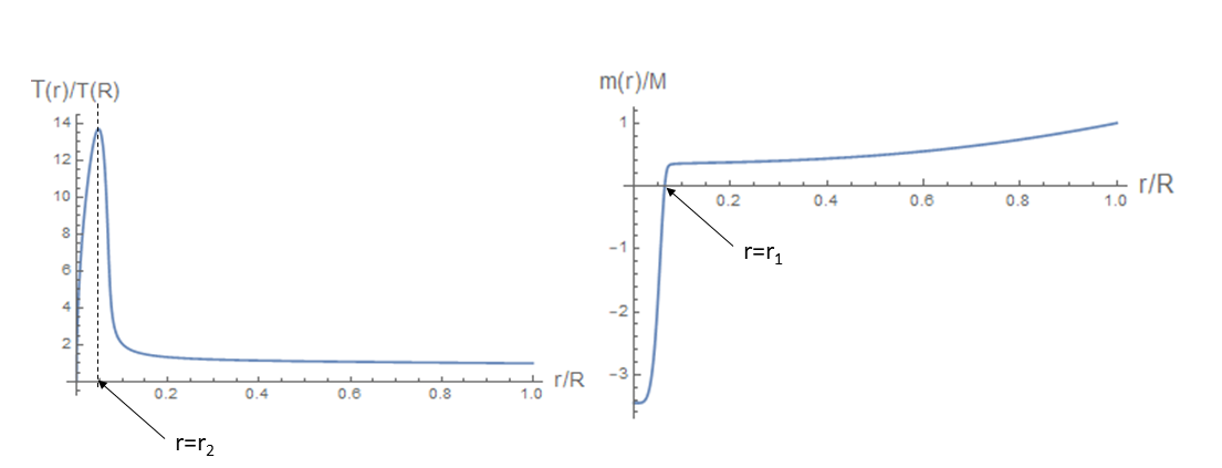
In the next section, we will discuss properties of the singular solution in more detail, emphasizing in particular the nature of the singularity at .
4 Properties of singular solutions
4.1 Relation to the negative-mass Schwarzschild singularity
As shown in the previous section, a singular solution to the TOV equations is characterized by for positive and by a lapse function that diverges as
| (55) |
for some constant . The two parameters and fully characterize the structure of the solutions near .
Around , the metric (31) becomes
| (56) |
The metric Eq. (56) has the same asymptotic behavior with a Schwarzschild solution with negative mass , modulo a time rescaling. Indeed, Eq. (56) can be expressed as
| (57) |
where .
Next we evaluate the sub-leading terms to and as . Since vanishes at least with as with fixed, grows at most with near . By Eq. (33), vanishes at least with . Hence, , where and .
It follows that the metric component
| (58) |
is equal with the metric component of a negative-mass Schwarzschild geometry, up to terms of order . The first matter-dependent term appears at order or higher.
Eq. (35) implies that near
| (59) |
Since grows at most with near zero, Eq. (59) becomes
| (60) |
up to terms of order at least . Hence,
| (61) |
This means that for , the metric corresponds to a vacuum solution of Einstein’ equation. There is little matter in the vicinity of the singularity.
The curvature around can be calculated using the negative-mass Schwarzschild spacetime. This means that the Ricci tensor vanishes, while the Kretschmann scalar is given by
| (62) |
Hence, is a curvature singularity, and it is naked as it is not covered by any horizon.
We also note that the area to volume ratio of a small sphere of area around , decreases with , while the same quantity around a regular point decreases with .
4.2 Geodesics near the singularity
Next, we analyze the properties of the singularity at in relation to the causality and predictability properties of the spacetime. To this end, we study the geodesic equation near ,
| (63) |
where and are constants. For causal geodesics, correspond to energy per unit mass and it satisfies
| (64) |
is the angular momentum per unit mass, and it satisfies . The parameter takes the value for timelike, for spacelike and for null geodesics. The dot denotes derivative with respect to an affine parameter that increases towards the future direction.
The singularity strongly repulses all test particles. No timelike geodesics arrive at the singularity. Incoming massive particles reach at most up to a minimal radius, (achieved for ), and then they bounce back. Hence, all timelike geodesics that start from past timelike infinity reach the future timelike infinity . The spacetime is timelike geodesically complete.
Null geodesics with also reach a minimal radius . The only causal geodesics that reach the singularity are radial () null geodesics, and these form a set of measure zero in the space of all null geodesics. These satisfy ; hence, , for a path parameter that vanishes at . By Eq. (64), , for some constant . The solution corresponds to outgoing geodesics and the solution to incoming geodesics.
In a recent analysis of the singularity in negative-mass Schwarzschild spacetime [30], the divergence of curvature at was given as a justification for the incompleteness of these geodesics. This statement presupposes that the point has been excised from the spacetime manifold. If, however, is treated as a spacetime boundary or ideal point in the sense of Geroch, Kronheimer and Penrose [29], we can interpret as the point where incoming future directed geodesic becomes outcoming future directed geodesics33 3 Contrast this situation with radial null geodesics in the positive-mass Schwarzschild spacetime. The only future-directed geodesics around , are of the form , because is a past-directed timelike vector field near . Incoming geodesics terminate at .. The radial geodesics are continuous but non-differentiable at , and they can be defined as the limit of differentiable geodesics with nonzero angular momentum , at the limit —see, Fig. 3. Hence, all null geodesics that start from the past null infinity end at the future null infinity .
Note that null geodesic propagation through takes place at finite time. Consider a static observer at and on the equatorial plane who sends a light ray towards the center. Consider also a mirror at and that reflects the outgoing ray. The initial observer will detect the reflected light ray after finite proper time that vanishes as .

To summarize, singular solutions to the TOV equations are causally complete. The only trouble at the level of causal geodesics is the non-differentiability of radial null geodesics at the singularity. Hence, the singularity at is much more benign than black hole singularities, despite its nakedness.
4.3 Bounded acceleration paths
Causal geodesic completeness is a minimal condition for a spacetime to be considered singularity-free [32]. Of course, observers are not necessarily free-falling, they may be accelerated. However, any spaceship moving towards the singularity can only have finite acceleration and it can carry only a finite amount of fuel. This implies that the physically relevant criterion is the completeness of bounded-acceleration trajectories [33]. We will study the singularity at in relation to this criterion.
The acceleration one-form for static observers near the singularity is
| (65) |
The minus sign in Eq. (65) implies a repulsive force. The proper acceleration diverges like as . In static configurations, infinite pressure is required in order to push a material element towards the singularity.
Next, we consider an infalling observer on a timelike curve with four-velocity . Since ,
| (66) |
If and are bounded, then
| (67) |
as . Hence, approximates the four-velocity of a static observer. By Eq. (65), the observer requires infinite acceleration to reach the singularity.
We examine the possibility that diverges as . Since the tangential acceleration does not affect whether the observer reaches the singularity or not, the divergence of or is irrelevant.
Let diverges with or more slowly. Then, Eq. (67) still applies and the earlier conclusion remains unchanged. If diverges faster that , then by Eq. (66),
| (68) |
However, this expression is not compatible with bounded acceleration. Taking for , we find that , hence, divergent.
We conclude that no observer with finite proper acceleration reaches the singularity. There are no incomplete timelike paths with bounded acceleration. The spacetime is bounded-acceleration complete.
This conclusion allows us to characterize the singularity at as an ideal point [29] in the following sense. Let be the set of all points in the past of along a timelike curve of bounded acceleration. Then, can be identified with part of the boundary of , where is the future timelike infinity. This characterization is compatible with the characterization of as a conformal boundary, to be presented next.
4.4 The surface as a conformal boundary
Consider a singular conformal transformation of a singular solution to the TOV equations. We choose . Around , the metric is
| (69) |
where and . The spacetime described by the metric (69) has a boundary at , and the pull-back of the four metric on is a Lorentzian metric. Hence, is a spacetime with timelike boundary [31].
The metric is ultrastatic. In ultrastatic spacetimes, causal geodesics correspond to geodesics of the pull-backed three metric
| (70) |
on the spatial manifold that is described by the local coordinates .
is a manifold with boundary. The boundary is defined by . A submanifold of constant is a two-sphere of area . The solid angle of a sphere of proper radius around goes to zero with .
The three-metric (70) has negative curvature near , and the Ricci scalar diverges as as . Despite the divergence of the curvature, curves can be continued across the singularity. In this sense, the boundary behaves like a conical singularity.
To see this, we first note that the singularity at is reached only by radial geodesics. These geodesics are complete, but they are not differentiable at the singularity. Furthermore, the proper distance of any point from the singularity is finite and equal to . We do not provide a proof of these statements, as they follow from an analysis that is almost identical to that of Sec. 4.2.
The key point is that the causal structure of an ultrastatic spacetime is Newtonian, with the time as a Newtonian time parameter. This is because the vector field is covariantly constant. This implies that all continuous timelike paths can be parameterized by , and that each (inextendible) path intersects a surface of constant only once. Hence, the spacetime is a globally hyperbolic spacetime with boundary [31].
A Penrose diagram for the spacetime is given in Fig. 4.

5 Limiting and pathological cases
In this section, we consider pathological behaviors that appear when integrating the TOV equations from the boundary inwards. By Thm. 1, these pathologies do not appear in systems with thermodynamically consistent EoS. We noted already that horizons can appear if we let pressure become negative. Here, we will focus on pathologies that arise by violating the thermodynamic integrability condition, and we will explain how they can be fixed.
5.1 Zero temperature solutions
The EoS employed in the study of compact stars often correspond to the limit of zero temperature. The limit is taken for constant , rather than for constant , resulting to a functional relation between pressure and density that is not integrable. In what follows, we will describe the thermodynamically consistent way of taking the limit in an equation of state, and describe the associated singular solutions to the TOV equations.
For concreteness, we will employ the original Oppenheimer-Volkoff EoS [17] that describes a single species of free fermions with mass . Since we consider a single species of fermions, we drop the index in and . The EoS for an ideal gas of free relativistic fermions is
| (71) | |||||
| (72) | |||||
| (73) |
where and . stands for the generalized Fermi integral
| (74) |
The regime of highly degenerate fermions corresponds to and . For and , is suppressed exponentially: . In Eq. (71—73), . We will employ the variable . Then, for .
It is convenient to view the thermodynamic variables (71—73) as functions of and . Hence, Eqs. (71—73) become
| (75) |
For , the functions drop sharply as decreases from to ; the width of the transition region is of order . In the limit , , and vanish for , while for we can use the approximation
| (76) |
In this limit, the functions and depend only on ,
| (77) | |||||
| (78) | |||||
| (79) |
The above expressions for and are the dominant terms in the thermodynamic variables at the limit of arbitrarily small (but non-vanishing) temperature, and arbitrarily large (but finite) . They are exact up to terms of order .
Next, we define the dimensionless variables , and , and we express Eqs. (32—34) as
| (80) | |||||
| (81) |
We integrate Eqs. (80—81) from the boundary inwards, for constant and with initial conditions (zero pressure at the stellar surface) and , where . The local temperature at the stellar surface is , hence,
| (82) |
By lemma 3, there is a point , such that for . The solution continues to , where . By continuity, there is a point , such that . For , and are exponentially suppressed as approaches the singularity. In fact, numerical integration stops before , because the values of and reach machine precision.
Integrating Eq. (80) from to , we obtain
| (83) |
where . Since for , in . For and , is an increasing function of at constant . Hence, in Eq. (83) is bounded above by . By Eq. (73), , where . We conclude that
| (84) |
As , becomes -independent and it is determined by using the limiting expressions (77—79) in the TOV equation (81). Hence, and coincide up to terms of order .
The total number of particles contained in the ball is
| (85) |
For , and . It follows that
| (86) |
Eqs. (84) and (86) imply that the spacetime geometry for can be approximated by a vacuum solution of Einstein’s equation, namely, Schwarzschild solution with negative mass , where . In this approximation, , and
| (87) |
for all . The approximation is accurate to order , and it becomes exact in the limit . Since , the limiting behavior of near leads to the identification
| (88) |

5.2 Non integrable EoS
Consider an EoS . If is a smooth function, non-integrability is due to the asymptotic behavior of at infinity or near zero. As shown in Sec. 2.4, if grows more slowly than a linear function at large , the energy density diverges at a finite value of temperature, say, . Hence, if the integration of the TOV equations leads to a value at some point (recall that is the point where becomes an increasing function), the energy density will diverge there.
This pathology is easy to fix, as it arises from the asymptotic behavior of the EoS as . We only have to modify the EoS for ultra-high temperatures, well beyond any regime that is currently known, so that condition (48) applies. Then, the density divergence at high densities will be removed.
In the opposite regime, the faster-than-linear vanishing of as leads to a zero for at finite temperature, say, . If appears in the integration of the TOV equations (usually at ), then the integration stops, as cannot take negative values. This is a very common behavior of many popular EoS employed in the study of compact stars. This is more difficult to correct, because the low density regime is familiar to us, and we cannot impose arbitrary mathematical conditions.
For concreteness, we will consider a popular EoS in the study of compact stars, that originates from Gratton [34]
| (89) |
where is a reference pressure and . The EoS (89) is polytropic at densities smaller than ; where is the usual polytropic index. For , the EoS describes radiation.
We solve Eq. (12) to obtain
| (90) | |||||
| (91) |
where is an integration constant. For , . Hence, for Gratton’s EoS leads the integration of the TOV equations towards the center stops at a value of where the temperature is reached.
To correct this behavior we need to extrapolate Eqs. (90) and (91) to . Gratton’s EoS is supposed to describe fermionic degenerate matter, so the limit of low densities (and temperature) essentially describes a cold dilute gas of fermions of mass . The latter is given by Eqs. (20—22). Hence, we need to connect Eqs. (90) and (91), with the EoS for a dilute gas
| (92) |
for some constant . Since , it suffices to connect the functions at some point . Since we have two parameters and , we can always choose and its first derivative to be continuous at .
In the EoS for a cold dilute gas of fermions, pressure and energy density drop exponentially as as temperature decreases. In this sense, the condition is analogous to the condition of the model in Sec. 5.1. Hence, we can treat the associated solutions to the TOV equation the same way. Let be a point such that in a solution. The total mass contained in the ball is suppressed by a factor . If , it is a good approximation to treat the solution in as a vacuum solution, with negative mass given by . Hence, we will obtain a solution similar to that of Fig. (5).
6 Dynamical stability
The vanishing of the pressure at the center of a singular solution to the TOV equation may appear counter intuitive, when compared with the usual insight that compact stars are stabilized as a result of high central pressure. Indeed, one would expect that all solutions with positive pressure gradients are dynamically unstable. However, this physical intuition follows from the study of regular solutions. Singular solutions have the novel feature that the singularity repulses the interior matter layers. The issue is whether this repulsion suffices to compensate for the lack of central pressure, as fa stability is concerned. In this section, we undertake a preliminary investigation of this issue, by studying adiabatic radial perturbations.
6.1 Adiabatic radial perturbations
A stationary solution to Einstein’s equations is (linearly) dynamically stable, if no linearized perturbation admits runaway solutions. Here, we discuss radial perturbations that are typically characterized by the strongest instabilities.
Consider spherically symmetric metrics of the form
| (93) |
with time-dependent lapse and mass function that perturb a static solution to Einstein’s equations.
The linearized perturbations to Einstein’s equation can be expressed in terms of an appropriately chosen function that satisfies a hyperbolic equation [23, 24]
| (94) |
where and are functions of that are determined by the equilibrium solution. A dot denotes differentiation with respect to and a prime denotes differentiation with respect to .
For adiabatic perturbations, the functions and are given by [23]
| (95) | |||||
| (96) | |||||
| (97) |
where refer to the equilibrium solution; is the fluid’s adiabatic index.
For oscillatory perturbations with frequency , Eq. (94) becomes
| (98) |
Eq. (98) is a Sturm-Liouville equation. The usual boundary conditions for are , and [23]. For these boundary conditions, the Sturm-Liouville operator , defined by is self-adjoint. Hence, its eigenvalue are real valued.
Suppose we order the eigenvalues of as . A negative eigenvalue signifies a mode growing unboundedly; hence, dynamical instability. It follows that is a necessary and sufficient condition for dynamical stability.
The smallest eigenvalue can be determined from a variational principle,
| (99) |
where is the Rayleigh-Ritz functional
| (100) |
The minimum in Eq. (99) is taken over the set of all differentiable function , with finite , that satisfy the boundary conditions. Hence, dynamical stability requires that
| (101) |
for any .
It is well known that in regular solutions, instability appears at high central temperatures and pressures. This can be seen from the ratio as ,
| (102) |
where we use the overbar to denote the value of a variable at the center.
This ratio gives the strength of the negative contribution to near the center. In contrast, the ratio as is proportional to , and it is bounded with increasing central temperature. This suggests that for solutions with sufficiently large central temperature, the negative contribution from dominates, and negative eigenvalues occur.
6.2 Enhanced stability
The behavior of the Rayleigh-Ritz functional is very different for singular solutions. First, we note that for solutions to the TOV equations, implies that . Indeed, the latter inequality is equivalent to , which is always valid, because for . It follows that for .
The function remains negative up to a point . The point can be characterized by , where on it; varies between 0 at and 2 at . Substituting Eq. (42) into Eq. (97), we find that has the same sign with the quantity
| (103) |
This quantity is always positive if and . It is always negative if and . Combining these inequalities, we find that lies between and . It follows that remains negative in a large neighborhood of the maximum-temperature point .
We conclude that the interior layers of the singular solution () always contribute a positive term to the Rayleigh-Ritz functional. Hence, the repulsive singularity at the center enhances dynamical stability. Dynamical instability necessitates a negative contribution to the Rayleigh-Ritz functional from that overcome the positive contributions from the inner layers. This is possible if the maximum value of is very close to unity, as grows with and with . Hence, instabilities are correlated with the existence of surfaces of high blue-shift in the outer layers. Since many singular solutions do not have such surfaces, we expect that stable singular solutions are generic.
6.3 An example
As an example, we consider the stability of the solutions that were studied in Sec. 5.1. At the limit of very large , the -dependence factors out, so that the space of solutions is two-dimensional. We parameterize this space by the dimensionless mass and the compactness . Regular solution define an one-dimensional submanifold of that is plotted in Fig. 5.
The OV limit for this model corresponds to . For , there are no regular solutions. For , there are regular solutions. For , there is only one regular solution for each , for there are more than one solutions.
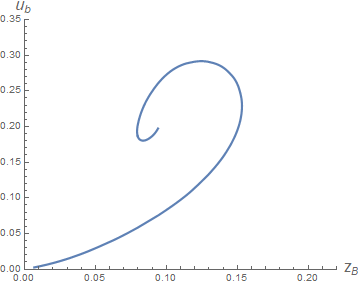
We constructed the Reyleigh-Ritz functional for this class of solutions. For each , we estimated the smallest eigenvalue using a variational method. We found it convenient to employ the function
| (104) |
If , then the solution with is stable, otherwise, it is unstable. In Fig. 6, we plot as a function of for representative values of .

Our conclusions from the numerical study of are the following.
- 1.
For all , the solutions are stable for sufficiently small , and unstable for sufficiently large .
- 2.
For , there is one or more islands of stability between regions of that describe unstable solutions.
- 3.
For , is discontinuous at points that correspond to regular solutions.
- 4.
For , is continuous, and there is a single point of transition from stable to unstable solutions.
6.4 Thermodynamical stability
A solution to the TOV equation is physically meaningful if it is both dynamically and thermodynamically relevant. We showed that dynamical stability is plausible for singular solutions, even though the analysis of more general types of perturbation are needed. Thermodynamic stability is a more complex issue, in fact, the thermodynamic consistency of solutions to the TOV equation is one of the main motivations for this work [3].
We will undertake the thermodynamic analysis in a future work. The reason is that such an analysis requires the introduction of entropy associated to the singularity [3]. The arguments in support for this singularity entropy goes beyond the scope of this work, and it does involve a degree of conjecture, as it goes beyond classical General Relativity. We only note that such an analysis was undertaken in Ref. [3] for self-gravitating radiation. There, it was shown that singular solutions are not thermodynamically stable for masses smaller than the Oppenheimer-Volkoff limit , and that some thermodynamically stable singular solutions exist for . We believe that this result can be generalized to all solutions of the TOV equation that were considered in this paper.
7 Conclusions
Our results provide a complete characterization of all solutions to the TOV equation, including singular ones. All singular solutions share the same structure and have a curvature singularity at the center. The singularity strongly repulses any matter that approaches it. The repulsion enhances stability, and also results to only a subset of measure zero of all geodesics reaching the singularity.
We will explore the possibility that singular solutions to the TOV equations correspond to actual astrophysical objects in a different publication. Here, we summarize the reasons why these solutions are of significant interest. They are generic solutions a paradigmatic equation of relativistic astrophysics, and for this reason, it is natural to expect that they appear in final stages of gravitational collapse. They describe a geometry in which a region with matter interpolates between a negative-mass Schwarzschild spacetime at the center to a positive-mass Schwarzschild spacetime at infinity. They provide an tractable model of a spacetime with timelike singularity that is bounded acceleration complete. Their stability analysis is intriguingly novel: stability is enhanced by the repulsive singularity at the center and it is disrupted by high blue-shift surfaces at the outer layers of the solution.
References
- [1] W. H. Zurek and D. N. Page, Black-hole Thermodynamics and Singular Solutions of the Tolman-Oppenheimer-Volkoff Equation, Phys. Rev. D29, 628 (1984).
- [2] G. L. Comer and J. Katz, Some Conditions for Existence of Tension Stars, MNRAS 267, 51 (1994).
- [3] C. Anastopoulos and N. Savvidou, Entropy of Singularities in Self-Gravitating Radiation, Class. Quant. Grav. 29, 025004 (2012).
- [4] C. Anastopoulos and N. Savvidou, The Thermodynamics of a Black Hole in Equilibrium Implies the Breakdown of Einstein Equations on a Macroscopic Near-Horizon Shell, JHEP 144 (2016).
- [5] H. C. Kim, Classifying Self-Gravitating Radiations, Phys. Rev. D 95, 044021 (2017).
- [6] R. Penrose, Singularities and Time-Asymmetry, in Einstein Centenary Volume, S. W. Hawking and G. Ellis (eds.) (Cambridge University Press, Cambridge 1979).
- [7] R. Penrose, The Problem of Spacetime Singularities: Implications for Quantum Gravity?, in The Future of Theoretical Physics and Cosmology, G. Gibbons, P. Shellard and S. Rankin (eds.) (Cambridge University Press, Cambridge 2002).
- [8] D. M. Eardley and L. Smarr, Time Functions in Numerical Relativity: Marginally Bound Dust Collapse,Phys. Rev. D19, 2239 (1979).
- [9] D. Christodoulou, Violation of Cosmic Censorship in the Gravitational Collapse of a Dust Cloud, Commun. Math. Phys. 93, 171 (1984).
- [10] P. S. Joshi, Gravitational Collapse and Spacetime Singularities (Cambridge University Press, Cambridge 2007).
- [11] P. S. Joshi and D. Malafarina, Recent Developments in Gravitational Collapse and Spacetime Singularities, Int. J. Mod. Phys. D20, 2641 (2011).
- [12] H. B. Callen, Thermodynamics and an Introduction to Thermostatistics (John Wiley, New York, 1985).
- [13] J. Katz and Y. Manor, Entropy Extremum of Relativistic Self-Bound Systems: A Geometric Approach, Phys. Rev. D12, 956 (1975).
- [14] N. Savvidou and C. Anastopoulos, The Thermodynamics of Self-gravitating Systems in Equilibrium is Holographic, Class. Quant. Grav. 31, 055003 (2014).
- [15] K. Huang, Statistical Mechanics, 2nd ed. (Wiley, 1987).
- [16] R. C. Tolman, Static Solutions of Einstein’s Field Equations for Spheres of Fluid, Phys. Rev. 55, 364 (1939).
- [17] J.R. Oppenheimer and G.M. Volkoff, On Massive Neutron Cores, Phys. Rev. 55, 374 (1939).
- [18] H. A. Buchdahl, General Relativistic Fluid Spheres, Phys. Rev. 116, 1027 (1959).
- [19] H. Andreasson, Sharp Bounds on of General Spherically Symmetric Static Objects, J. Diff. Equations 245, 2243 (2008); P. Karageorgis and J. Stalker, Sharp bounds on 2m/r for static spherical objects, Class. Quant. Grav. 25, 195021 (2008).
- [20] N. Dadhich, Buchdahl Compactness Limit and Gravitational Field Energy, JCAP 04, 035 (2020).
- [21] J. Smoller and B. Temple, On the Oppenheimer‐Volkoff Equations in General Relativity, Arch. Rational Mech. Anal. 142, 177 (1998).
- [22] E. A. Coddington and N. Levinson, Theory of Ordinary Differential Equations (McGraw-Hill, New York, 1955).
- [23] C. W. Misner, K. S. Thorne and J. A. Wheeler, Gravitation (W. H. Freeman and Co, 1973).
- [24] S. Yabushita, Pulsational Instability of Isothermal Gas Spheres within the Framework of General Relativity, Mon. Not. R. Astron. Soc. 165, 17 (1973).
- [25] L. D. Landau and E. M. Lifshitz, The Classical Theory of Fields, 4th edition (Pergamon Press, 1975), pg. 87.
- [26] Y. B. Zel’dovich, Equation of State at a Superhigh Density and Relativistic Restrictions, JETP 41, 1609 (1961).
- [27] R. P. Geroch and D. J. Hegyi, Relativistic Equations of State, Nature 215, 501 (1967).
- [28] Y. B. Zel’dovich, The equation of state at ultrahigh densities and its relativistic limitations, Soviet Phys. JETP 14, 1143 (1962); Y. B. Zel’dovich, A hypothesis, unifying the structure and the entropy of the Universe, Mon. Not. R. Astron. Soc. 160, 1 (1972).
- [29] R. Geroch , E. H. Kronheimer and R. Penrose, Ideal points in space-time, Proc. Roy. Soc. A327, 545 (1972).
- [30] S. Vargas-Serdio and H. Quevedo, Singularity Theorems in Schwarzschild Spacetimes, Eur. Phys. J. Plus 135, 636 (2020).
- [31] A. L. Hau, J. L. Flores and M. Sanchez, Structure of globally hyperbolic spacetimes with timelike boundary, Rev. Mat. Iberoam, doi: 10.4171/rmi/1201 [arXiv:1808.04412].
- [32] S. W. Hawking and G. R. F. Ellis, The Large Scale Structure of Spacetime (Cambridge University Press, Cambridge 1973).
- [33] R. P. Geroch, What is a Singularity in General Relativity?, Ann. Phys. (New York), 48, 526 (1968).
- [34] L. Gratton, Rend. Accad. Nasionale dei Lincei 38, 354 (1964).