跳到论文正文
W Papers独立论文阅读器 arXiv:2010.02126 论文正文 计算阅读时间 · 0%
引用这篇论文根据当前论文元数据生成,正式投稿前建议核对。


License: arXiv.org perpetual non-exclusive license
arXiv:2010.02126v4 [math.ST] 25 Sep 2022

Bayesian Fixed-domain Asymptotics for Covariance Parameters in a Gaussian Process Model

Cheng Li Thanks: stalic@nus.edu.sg Affiliation: Department of Statistics and Data Science, National University of Singapore
Abstract

Gaussian process models typically contain finite dimensional parameters in the covariance function that need to be estimated from the data. We study the Bayesian fixed-domain asymptotics for the covariance parameters in a universal kriging model with an isotropic Matérn covariance function, which has many applications in spatial statistics. We show that when the dimension of domain is less than or equal to three, the joint posterior distribution of the microergodic parameter and the range parameter can be factored independently into the product of their marginal posteriors under fixed-domain asymptotics. The posterior of the microergodic parameter is asymptotically close in total variation distance to a normal distribution with shrinking variance, while the posterior distribution of the range parameter does not converge to any point mass distribution in general. Our theory allows an unbounded prior support for the range parameter and flexible designs of sampling points. We further study the asymptotic efficiency and convergence rates in posterior prediction for the Bayesian kriging predictor with covariance parameters randomly drawn from their posterior distribution. In the special case of one-dimensional Ornstein-Uhlenbeck process, we derive explicitly the limiting posterior of the range parameter and the posterior convergence rate for asymptotic efficiency in posterior prediction. We verify these asymptotic results in numerical experiments.

Keywords: Fixed-domain asymptotics, Limiting posterior distribution, Matérn covariance function, Asymptotic efficiency in posterior prediction

1 Introduction

Gaussian processes (GP) have been widely used in spatial statistics, computer experiments, machine learning, and many other fields. In this paper, we consider the observation from the following spatial Gaussian process regression model, known as the universal kriging model (Chapter 3 Section 3.4, Cressie 1993):

Y⁡(si)\displaystyle Y(s_{i}) =m(si)⊤β+X(si),for i=1,…,n.\displaystyle=\mathrm{m}(s_{i})^{\top}\beta+X(s_{i}),\quad\text{for }i=1,\ldots,n. (1)

In the model (1), 𝒮n={s1,…,sn}\Scal_{n}=\{s_{1},\ldots,s_{n}\} is a sequence of distinct sampling points in the fixed domain 𝒮=[0,T]d\Scal=[0,T]^{d}, and 0<T<∞0<T<\infty is a known constant and the dimension d∈{1,2,3}d\in\{1,2,3\}. Such a dimension dd is of primary interest in spatial statistics. Here m⁡(⋅)=(m1​(⋅),…,mp​(⋅))⊤\mathrm{m}(\cdot)=(\mathrm{m}_{1}(\cdot),\ldots,\mathrm{m}_{p}(\cdot))^{\top} is a pp-dimensional vector of linearly independent and known deterministic functions defined on 𝒮\Scal, and β∈ℝp\beta\in\mathbb{R}^{p} is the regression coefficient vector. In applications, m1,…,mp\mathrm{m}_{1},\ldots,\mathrm{m}_{p} can include the constant function 11, and hence β\beta can include an intercept term. In the model (1), X⁡(⋅)X(\cdot) is a mean-zero Gaussian stochastic process X={X⁡(s):s∈𝒮}X=\left\{X(s):s\in\Scal\right\}. We assume that the covariance function of XX is the isotropic Matérn covariance function given by

Cov(X⁡(s),X⁡(t))\displaystyle\Cov(X(s),X(t)) =σ2​Kα,ν​(s−t)=σ2​21−νΓ⁡(ν)​(α​‖s−t‖)ν​𝒦ν⁡(α​‖s−t‖),\displaystyle=\sigma^{2}K_{\alpha,\nu}(s-t)=\sigma^{2}\frac{2^{1-\nu}}{\Gamma(\nu)}\left(\alpha\|s-t\|\right)^{\nu}\Kcal_{\nu}\left(\alpha\|s-t\|\right), (2)

for any s,t∈𝒮s,t\in\Scal, where ν>0\nu>0 is the smoothness parameter, σ2>0\sigma^{2}>0 is the variance (or partial sill) parameter, and α>0\alpha>0 is the inverse range (or length-scale) parameter, 𝒦ν⁡(⋅)\Kcal_{\nu}(\cdot) is the modified Bessel function of the second kind (Kreh 2012), and ∥⋅∥\|\cdot\| is the Euclidean norm. The Matérn covariance function is popular in applications of spatial statistics and computer experiments because the smoothness parameter ν\nu provides flexibility in controlling the smoothness of sample paths (Stein 1999a). The observed data from the model (1) are Yn=(Y⁡(s1),…,Y⁡(sn))⊤Y_{n}=(Y(s_{1}),\ldots,Y(s_{n}))^{\top}. Parameter estimation and prediction of Y⁡(⋅)Y(\cdot) at a new spatial location (known as kriging) is based on YnY_{n}. For simplicity, we call α\alpha the range parameter in the rest of the paper.

In Bayesian inference on GP models (Handcock and Stein 1993, De Oliveira et al. 1997), it is common practice to assign prior distributions on the regression coefficient β\beta and the covariance parameters (σ2,α)(\sigma^{2},\alpha), and the prediction of Y⁡(s∗)Y(s^{*}) at a new location s∗s^{*} is based on the posterior distribution of (β,σ2,α)(\beta,\sigma^{2},\alpha). There is abundant literature in Bayesian spatial statistics on speeding up the costly GP posterior computation for spatial datasets with a large sample size nn (Banerjee et al. 2008, Sang and Huang 2012, Datta et al. 2016, Guhaniyogi et al. 2022, Heaton et al. 2019, etc.) However, there is a clear lack of theoretical understanding of the asymptotic properties of the Bayesian posterior distributions of covariance parameters (σ2,α)(\sigma^{2},\alpha). This theory is important because in Bayesian inference, instead of taken as fixed values, the covariance parameters (σ2,α)(\sigma^{2},\alpha) are randomly drawn from their posterior using sampling algorithms such as Markov chain Monte Carlo (MCMC), which eventually affect the posterior prediction performance of the GP model.

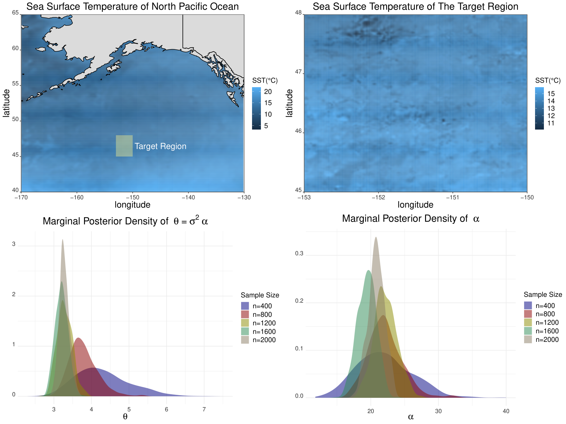
To illustrate our motivation, we fit a Bayesian universal kriging model in (1) to the sea surface temperature (SST) data. The data is obtained from National Oceanographic Data Centres (NODC) World Ocean Database (https://www.ncei.noaa.gov/products/world-ocean-database) and the entire data corresponds to sea surface temperature measured by remote sensing satellites on 16th August 2016. The data we test come from the Pacific Ocean between 45∘45^{\circ}–48∘48^{\circ} north latitudes and 150∘150^{\circ}–153∘153^{\circ} west longitudes. The original dataset is high-resolution on a 0.025∘×0.025∘0.025^{\circ}\times 0.025^{\circ} fine grid. We choose subsets of size {400,800,1200,1600,2000}\{400,800,1200,1600,2000\} on equispaced grids. For the regressors m⁡(⋅)\mathrm{m}(\cdot), we include all p=10p=10 monomials of the latitude and longitude up to degree 3, since on average SST is lower at higher latitudes. We set ν=1/2\nu=1/2, and assign a flat prior π⁡(β)∝1\pi(\beta)\propto 1 on β\beta, an inverse gamma prior with shape and rate parameters both equal to 2 on σ2\sigma^{2} and an independent Uniform​(0.01,300)\text{Uniform}(0.01,300) prior on α\alpha. The marginal posterior densities of α\alpha and θ=σ2​α\theta=\sigma^{2}\alpha are shown in Figure 1 below. As the sample size increases, the marginal posterior density of the parameter θ=σ2​α\theta=\sigma^{2}\alpha seems to contract faster with nn than that of the range parameter α\alpha. Even with sample size n=2000n=2000, the posterior of α\alpha still has a relatively large uncertainty. It is natural to ask the following questions: (i) Do the posteriors of (σ2,α)(\sigma^{2},\alpha) (or (θ,α)(\theta,\alpha)) converge, and if so, at what rates? (ii) How does the posterior uncertainty in (σ2,α)(\sigma^{2},\alpha) affect the posterior prediction of the response Y⁡(⋅)Y(\cdot) at a new location?

Refer to caption
Figure 1: Example of the Sea Surface Temperature (SST) data. Top left: The SST data in North Pacific Ocean and the target region of our sampled data. Top right: The SST data in the target region. Bottom left: The marginal posterior densities of θ=σ2​α\theta=\sigma^{2}\alpha for sample sizes n=400,800,1200,1600,2000n=400,800,1200,1600,2000. Bottom right: The marginal posterior densities of α\alpha for sample sizes n=400,800,1200,1600,2000n=400,800,1200,1600,2000. The posterior densities are based on 2000 MCMC draws.

We provide an answer to (i) by studying the limiting posterior distributions of the covariance parameters (σ2,α)(\sigma^{2},\alpha) in the Matérn covariance function in (2), under the fixed-domain asymptotics (or infill asymptotics) framework (Stein 1988, Stein 1999a, Zhang 2004). We further answer (ii) and show that the randomness in (σ2,α)(\sigma^{2},\alpha) in general does not affect the posterior prediction performance. To the best of our knowledge, this paper is the first theoretical work on the fixed-domain asymptotics for the Bayesian posterior distribution of the finite dimensional parameters in Gaussian process covariance functions. In the following, we explain the reasons we adopt the fixed-domain asymptotics regime and the main technical challenges.

1.1 Why fixed-domain asymptotics?

In the fixed-domain asymptotics regime, the domain 𝒮\Scal remains fixed and bounded regardless of the increasing sampling size nn. This implies that as nn goes to infinity, the sampling points 𝒮n\Scal_{n} become increasingly dense in the domain 𝒮\Scal, leading to increasingly stronger dependence between adjacent observations in YnY_{n}. Besides the fixed-domain asymptotics regime, there are also increasing-domain asymptotics (Mardia and Marshall 1984) and mixed-domain asymptotics (Chang et al. 2017), in which the domain is assumed to increase as nn goes to infinity and therefore the minimum distance between two adjacent sampling points is either not decreasing or decreasing slowly with nn.

Compared to these alternatives, the fixed-domain setup has several advantages. First and foremost, a fixed domain matches up with the reality in many spatial applications. The advances in remote sensing technology make it possible to collected spatial data in larger volume and higher resolution in a given region (Sun et al. 2018). The motivating example above of the SST data from NODC has millions of observations with high-resolution on the 0.025∘×0.025∘0.025^{\circ}\times 0.025^{\circ} fine grid (about 2∼42\sim 4km range). Second, since the model (1) has a stationary Matérn covariance function, this stationarity assumption of GP is more likely to hold on a fixed domain rather than an expanding domain. Therefore, the fixed-domain asymptotics regime is more suitable for interpolation of spatial processes; see Section 3.3 of Stein 1999a for a cogent argument. Third, Zhang and Zimmerman 2005 has shown that the fixed-domain asymptotics has better parameter estimation performance than the increasing-domain asymptotics.

1.2 What are the main difficulties in Bayesian fixed-domain asymptotics?

Theoretically, the increasingly stronger spatial dependence among the observed data YnY_{n} in fixed-domain asymptotics leads to a lack of consistent estimation for the covariance parameters (σ2,α)(\sigma^{2},\alpha) (Zhang 2004) and therefore poses significant challenges to theory development. When the dimension of sampling points d=1,2,3d=1,2,3, a well known fixed-domain asymptotics result Zhang 2004 says that it is only possible to consistently estimate the microergodic parameter θ=σ2​α2​ν\theta=\sigma^{2}\alpha^{2\nu} in an isotropic Matérn covariance function, but not the individual variance parameter σ2\sigma^{2} and the range parameter α\alpha. The microergodic parameter is defined to be the parameter that uniquely determines the Gaussian measure induced by a Gaussian process, such that different values of microergodic parameter will lead to mutually orthogonal Gaussian measures; see Section 6.2 of Stein 1999a for a detailed explanation on this definition. On the other hand, both the variance and range parameters (σ2,α)(\sigma^{2},\alpha) can be consistently estimated if d≥5d\geq 5, with the case of d=4d=4 still open (Anderes 2010). Nevertheless, the cases with d=1,2,3d=1,2,3 are of primary interest in spatial and spatiotemporal applications and will be our main focus.

The standard Bayesian asymptotic theory consists of results such as posterior consistency, posterior convergence rates, and the Bernstein-von Mises (BvM) theorem (Ghosal and van der Vaart 2017). For parametric models, the BvM theorem typically relies on the local asymptotic normality (LAN) condition and the existence of uniformly consistent tests; see for example, Chapter 10 in van der Vaart 1998. Since no consistent frequentist estimator exists for (σ2,α)(\sigma^{2},\alpha) under fixed-domain asymptotics, one cannot expect to establish posterior consistency for (σ2,α)(\sigma^{2},\alpha). Instead, we will consider the microergodic parameter θ=σ2​α2​ν\theta=\sigma^{2}\alpha^{2\nu} which can be consistently estimated, and reparametrize the covariance function (2) by (θ,α)(\theta,\alpha). Crowder 1976 is an early work on the asymptotic normality of maximum likelihood estimator (MLE) in the presence of dependent observations and nuisance parameters. We will establish the LAN condition for the microergodic parameter θ\theta, uniformly over a wide range of values of the “nuisance” range parameter α\alpha. Such a uniform LAN condition based on data with increasingly stronger dependence is new in the literature and differs significantly from the LAN in classic parametric models with independent or weakly dependent data. The asymptotic normality for microergodic parameter θ\theta is crucial and guarantees the posterior prediction performance of Y⁡(⋅)Y(\cdot) at a new location.

For Bayesian inference on the GP covariance parameters, the only theoretical work we are aware of is Shaby and Ruppert 2012, who have worked under the increasing-domain asymptotics regime and have established that the joint posterior of all parameters in the tapered covariance functions converges to a limiting normal distribution. This is similar to the classic BvM theorem since the dependence among data does not get stronger under increasing-domain asymptotics. A key assumption in Shaby and Ruppert 2012 is that the observed covariance matrix have lower and upper bounded eigenvalues, which no longer holds under fixed-domain asymptotics.

We define some universal notation. Let ℝ+=(0,+∞)\mathbb{R}^{+}=(0,+\infty). For two positive sequences ana_{n} and bnb_{n}, we use an⪯bna_{n}\preceq b_{n} and bn⪰anb_{n}\succeq a_{n} to denote the relation lim supn→∞an/bn<+∞\limsup_{n\to\infty}a_{n}/b_{n}<+\infty, and an≍bna_{n}\asymp b_{n} to denote the relation an⪯bna_{n}\preceq b_{n} and an⪰bna_{n}\succeq b_{n}. For any integers k,mk,m, we let IkI_{k} be the k×kk\times k identity matrix, 0k0_{k} and 1k1_{k} be the kk-dimensional column vectors of all zeros and all ones, 0k×m0_{k\times m} be the k×mk\times m zero matrix. For any generic matrix AA, c​AcA denotes the matrix of AA with all entries multiplied by the number cc, and |A||A| denotes the determinant of AA. If AA is positive semidefinite, then λmin​(A)\lambda_{\min}(A) and λmax​(A)\lambda_{\max}(A) denote the smallest and largest eigenvalues of AA. Let 𝒩⁡(μ,Σ)\Ncal(\mu,\Sigma) be the normal distribution with mean μ\mu and covariance matrix Σ\Sigma. Sometimes to highlight the random variable Z∼𝒩⁡(μ,Σ)Z\sim\Ncal(\mu,\Sigma), we also write 𝒩⁡(z,μ,Σ)\Ncal(z;\mu,\Sigma) and the normal measure as 𝒩⁡(dz,μ,Σ)\Ncal(\mathrm{d}z;\mu,\Sigma).

The remainder of the paper is organized as follows. In Section 2 we introduce the basic model setup and present the main theorems on limiting posterior distribution of covariance parameters under fixed-domain asymptotics. Section 3 presents the theory on asymptotic efficiency in posterior prediction. Section 4 presents some empirical results from simulation study to verify the main theory. Section 5 includes some discussion on further extensions. The technical proofs of all theorems, propositions, lemmas, corollaries and additional simulation results are in the Supplementary Material.

2 Limiting Posterior Distribution for Covariance Parameters

2.1 Bayesian Model Setup

We consider the Bayesian estimation of (β,σ2,α)(\beta,\sigma^{2},\alpha) in the model (1) based on the observed data YnY_{n}. Throughout the paper, we assume that the domain dimension satisfies d∈{1,2,3}d\in\{1,2,3\}, and that the smoothness parameter ν>0\nu>0 is fixed and known. Estimation of the smoothness parameter ν\nu is an important research topic with some recent developments in frequentist literature (Loh 2015, Loh et al. 2021), but is beyond the scope of the current paper. We let the true parameter values in the Matérn covariance function that generates XX be (σ02,α0)(\sigma^{2}_{0},\alpha_{0}) and let the true regression coefficient vector be β0\beta_{0}. We use the notation X∼GP(0,σ02​Kα0,ν)X\sim\gp(0,\sigma_{0}^{2}K_{\alpha_{0},\nu}) and hence Y∼GP(m⊤​β0,σ02​Kα0,ν)Y\sim\gp(\mathrm{m}^{\top}\beta_{0},\sigma_{0}^{2}K_{\alpha_{0},\nu}).

Let Yn=(Y⁡(s1),…,Y⁡(sn))⊤Y_{n}=(Y(s_{1}),\ldots,Y(s_{n}))^{\top}. Let MnM_{n} be the n×pn\times p matrix by stacking the row vectors m​(si)⊤\mathrm{m}(s_{i})^{\top} for i=1,…,ni=1,\ldots,n. Throughout the paper, we assume that MnM_{n} is a rank-pp matrix without loss of generality, since all our results are asymptotic with n→∞n\to\infty. Let RαR_{\alpha} be the implied n×nn\times n Matérn correlation matrix on 𝒮n\Scal_{n} indexed by α\alpha, whose (i,j)(i,j)th entry is Rα,i​j=Kα,ν​(si−sj)R_{\alpha,ij}=K_{\alpha,\nu}(s_{i}-s_{j}), for i,j∈{1,…,n}i,j\in\{1,\ldots,n\}. We omit the dependence of RαR_{\alpha} on ν\nu. The covariance matrix of XnX_{n} is then σ2​Rα\sigma^{2}R_{\alpha}. Therefore, the model (1) can be equivalently written as Yn=Mn​β+XnY_{n}=M_{n}\beta+X_{n}. The log-likelihood function based on YnY_{n} is

ℒn⁡(β,σ2,α)\displaystyle\Lcal_{n}(\beta,\sigma^{2},\alpha) =−n2​log⁡σ2−12​log⁡|Rα|−12​σ2​(Yn−Mn​β)⊤​Rα−1​(Yn−Mn​β).\displaystyle=-\frac{n}{2}\log\sigma^{2}-\frac{1}{2}\log|R_{\alpha}|-\frac{1}{2\sigma^{2}}(Y_{n}-M_{n}\beta)^{\top}R_{\alpha}^{-1}(Y_{n}-M_{n}\beta). (3)

We study the Bayesian posterior distribution based on the log-likelihood (3). We follow the common practice in Bayesian spatial modeling literature (Banerjee et al. 2008, Sang and Huang 2012, Datta et al. 2016, Guhaniyogi et al. 2022, Heaton et al. 2019, Peruzzi et al. 2022, etc.) and assign the conjugate normal prior on β\beta, given by

β|σ2,α∼𝒩⁡(0p,σ2​Ωβ−1),\displaystyle\beta~|~\sigma^{2},\alpha\sim\Ncal\big(0_{p},\sigma^{2}\Omega_{\beta}^{-1}\big), (4)

which uses a rescaling with σ2\sigma^{2}, and the prior precision matrix Ωβ∈ℝp×p\Omega_{\beta}\in\mathbb{R}^{p\times p} is assumed to be symmetric positive semidefinite. Here we can set the prior mean to be 0p0_{p} without any loss of generality. This is because if the prior is β|σ2,α∼𝒩⁡(μβ,σ2​Ωβ−1)\beta|\sigma^{2},\alpha\sim\Ncal(\mu_{\beta},\sigma^{2}\Omega_{\beta}^{-1}) and the prior mean is μβ≠0p\mu_{\beta}\neq 0_{p}, we can always define a new response variable Y′​(s)=Y⁡(s)−m​(s)⊤​μβY^{\prime}(s)=Y(s)-\mathrm{m}(s)^{\top}\mu_{\beta}, the new regression coefficient vector β′=β−μβ\beta^{\prime}=\beta-\mu_{\beta}, and rewrite the original model (1) as Y′​(s)=m​(s)⊤​β′+X⁡(s)Y^{\prime}(s)=\mathrm{m}(s)^{\top}\beta^{\prime}+X(s) for s∈𝒮s\in\Scal, where Y′​(s)Y^{\prime}(s) is still fully observable on 𝒮n\Scal_{n} given that m⁡(⋅)\mathrm{m}(\cdot) is observable and μβ\mu_{\beta} is known. Furthermore, we allow the precision matrix Ωβ\Omega_{\beta} to be arbitrarily small, leading to a prior of β\beta with arbitrarily large variance. In particular, all our later theory covers the extreme case of improper noninformative prior π⁡(β|σ2,α)∝1\pi(\beta|\sigma^{2},\alpha)\propto 1 (Berger et al. 2001, Gu et al. 2018), which corresponds to Ωβ=0p×p\Omega_{\beta}=0_{p\times p}. The joint posterior density of (β,σ2,α)(\beta,\sigma^{2},\alpha) is then π⁡(β,σ2,α|Yn)∝exp⁡{ℒn⁡(β,σ2,α)}​π​(β|σ2,α)​π​(σ2,α)\pi(\beta,\sigma^{2},\alpha|Y_{n})\propto\exp\{\Lcal_{n}(\beta,\sigma^{2},\alpha)\}\pi(\beta|\sigma^{2},\alpha)\pi(\sigma^{2},\alpha). Since π⁡(β|σ2,α)\pi(\beta|\sigma^{2},\alpha) is the normal prior density, it is straightforward to obtain the conditional posterior of β\beta:

β|σ2,α,Yn∼𝒩⁡(β~α,σ2​(Mn⊤​Rα−1​Mn+Ωβ)−1),\displaystyle\beta~|~\sigma^{2},\alpha,Y_{n}\sim\Ncal\left(\widetilde{\beta}_{\alpha},\sigma^{2}\big(M_{n}^{\top}R_{\alpha}^{-1}M_{n}+\Omega_{\beta}\big)^{-1}\right), (5)

where β~α=(Mn⊤​Rα−1​Mn+Ωβ)−1​Mn⊤​Rα−1​Yn\widetilde{\beta}_{\alpha}=\big(M_{n}^{\top}R_{\alpha}^{-1}M_{n}+\Omega_{\beta}\big)^{-1}M_{n}^{\top}R_{\alpha}^{-1}Y_{n} and the subscript is to highlight its dependence on α\alpha but not σ2\sigma^{2}. We can further integrate out β\beta and obtain the marginal posterior density of the covariance parameters (σ2,α)(\sigma^{2},\alpha). We write π⁡(σ2,α|Yn)∝exp⁡{ℒn⁡(σ2,α)}​π​(σ2,α)\pi(\sigma^{2},\alpha|Y_{n})\propto\exp\{\Lcal_{n}(\sigma^{2},\alpha)\}\pi(\sigma^{2},\alpha), where the restricted log-likelihood ℒn⁡(σ2,α)\Lcal_{n}(\sigma^{2},\alpha) is given by

ℒn⁡(σ2,α)\displaystyle\Lcal_{n}(\sigma^{2},\alpha) =−12​σ2​Yn⊤​[Rα−1−Rα−1​Mn​(Mn⊤​Rα−1​Mn+Ωβ)−1​Mn⊤​Rα−1]​Yn\displaystyle=-\frac{1}{2\sigma^{2}}Y_{n}^{\top}\left[R_{\alpha}^{-1}-R_{\alpha}^{-1}M_{n}\big(M_{n}^{\top}R_{\alpha}^{-1}M_{n}+\Omega_{\beta}\big)^{-1}M_{n}^{\top}R_{\alpha}^{-1}\right]Y_{n}
−n−p2​log⁡σ2−12​log|Rα|−12​log⁡|Mn⊤​Rα−1​Mn+Ωβ|.\displaystyle\quad-\frac{n-p}{2}\log\sigma^{2}-\frac{1}{2}\log|R_{\alpha}|-\frac{1}{2}\log\big|M_{n}^{\top}R_{\alpha}^{-1}M_{n}+\Omega_{\beta}\big|. (6)

In spatial statistical theory, it is well known (Zhang 2004) that the parameters (σ2,α)(\sigma^{2},\alpha) cannot be consistently estimated under fixed-domain asymptotics. The main reason is that for two Gaussian measures GP(0,σj2​Kαj,ν)\gp(0,\sigma_{j}^{2}K_{\alpha_{j},\nu}) (j=1,2j=1,2) on the space of sample paths on the domain 𝒮=[0,T]d\Scal=[0,T]^{d} and d∈{1,2,3}d\in\{1,2,3\}, they are equivalent (or mutually absolutely continuous) as long as σ12​α12​ν=σ22​α22​ν\sigma_{1}^{2}\alpha_{1}^{2\nu}=\sigma_{2}^{2}\alpha_{2}^{2\nu}, and they are orthogonal otherwise. As a result, one cannot tell from a finite sample which parameter values (σj2,αj)(\sigma_{j}^{2},\alpha_{j}) (j=1,2j=1,2) are correct. Empirically, this phenomenon has been also observed (Anderes 2010, Fuglstad et al. 2019). Despite the lack of consistent estimator for (σ2,α)(\sigma^{2},\alpha), the microergodic parameter θ=σ2​α2​ν\theta=\sigma^{2}\alpha^{2\nu} can still be consistently estimated (Zhang 2004). For a fixed α>0\alpha>0, we maximize ℒn⁡(σ2,α)\Lcal_{n}(\sigma^{2},\alpha) with respect to σ2\sigma^{2} (and so θ\theta) to derive the restricted maximum likelihood estimator (REML), given by

σ~α2\displaystyle\widetilde{\sigma}^{2}_{\alpha} =1n−p​Yn⊤​[Rα−1−Rα−1​Mn​(Mn⊤​Rα−1​Mn+Ωβ)−1​Mn⊤​Rα−1]​Yn,θ~α=α2​ν​σ~α2.\displaystyle=\frac{1}{n-p}Y_{n}^{\top}\left[R_{\alpha}^{-1}-R_{\alpha}^{-1}M_{n}\big(M_{n}^{\top}R_{\alpha}^{-1}M_{n}+\Omega_{\beta}\big)^{-1}M_{n}^{\top}R_{\alpha}^{-1}\right]Y_{n},~~\widetilde{\theta}_{\alpha}=\alpha^{2\nu}\widetilde{\sigma}^{2}_{\alpha}. (7)

In (7), we have slightly extended the meaning of REML such that we can account for general prior precision matrix Ωβ\Omega_{\beta}, including the special case of Ωβ=0p×p\Omega_{\beta}=0_{p\times p} where β\beta can be viewed as normal random effects of m⁡(⋅)\mathrm{m}(\cdot), such that σ~α2\widetilde{\sigma}^{2}_{\alpha} (and θ~α\widetilde{\theta}_{\alpha}) can be viewed as the conventional REML of σ2\sigma^{2} (and θ\theta) in random effects models. We can plug in θ~α\widetilde{\theta}_{\alpha} in (3) to obtain the profile restricted log-likelihood of α\alpha (up to an additive constant), which plays an important role in our theory:

ℒ~n​(α)\displaystyle\widetilde{\Lcal}_{n}(\alpha) ≡ℒn⁡(α−2​ν​θ~α,α)\displaystyle\equiv\Lcal_{n}(\alpha^{-2\nu}\widetilde{\theta}_{\alpha},\alpha)
=−n−p2​log⁡{1n−p​Yn⊤​[Rα−1−Rα−1​Mn​(Mn⊤​Rα−1​Mn+Ωβ)−1​Mn⊤​Rα−1]​Yn}\displaystyle=-\frac{n-p}{2}\log\left\{\frac{1}{n-p}Y_{n}^{\top}\left[R_{\alpha}^{-1}-R_{\alpha}^{-1}M_{n}\big(M_{n}^{\top}R_{\alpha}^{-1}M_{n}+\Omega_{\beta}\big)^{-1}M_{n}^{\top}R_{\alpha}^{-1}\right]Y_{n}\right\}
−12​log⁡|Rα|−12​log⁡|Mn⊤​Rα−1​Mn+Ωβ|−n−p2.\displaystyle\quad-\frac{1}{2}\log\left|R_{\alpha}\right|-\frac{1}{2}\log\big|M_{n}^{\top}R_{\alpha}^{-1}M_{n}+\Omega_{\beta}\big|-\frac{n-p}{2}. (8)

The frequentist asymptotic normality for the MLE of θ\theta has been studied for the model (1) without the regression term, i.e., Y⁡(⋅)≡X⁡(⋅)∼GP(0,σ2​Kα,ν)Y(\cdot)\equiv X(\cdot)\sim\gp(0,\sigma^{2}K_{\alpha,\nu}). For this simplified model, Ying 1991 first studied the special case of d=1d=1 and ν=1/2\nu=1/2, followed by Zhang 2004, Du et al. 2009, Wang and Loh 2011, and Kaufman and Shaby 2013 for a general ν>0\nu>0. If α∈[α1,α2]\alpha\in[\alpha_{1},\alpha_{2}] for some constants 0<α1<α2<∞0<\alpha_{1}<\alpha_{2}<\infty, the MLE of θ\theta, denoted by θ^\widehat{\theta}, satisfies that n​(θ^−θ0)​→𝒟​𝒩​(0,2​θ02)\sqrt{n}(\widehat{\theta}-\theta_{0})\overset{\Dcal}{\rightarrow}\mathcal{N}(0,2\theta_{0}^{2}) as n→∞n\to\infty under fixed-domain asymptotics, where θ0=σ02​α02​ν\theta_{0}=\sigma_{0}^{2}\alpha_{0}^{2\nu} is the true value, and →𝒟\overset{\Dcal}{\rightarrow} is the convergence in distribution.

We study the fixed-domain asymptotic limit for the Bayesian posterior distribution of (σ2,α)(\sigma^{2},\alpha) based on the log-likelihood (2.1). We reparametrize the model using (θ,α)(\theta,\alpha), with θ=σ2​α2​ν\theta=\sigma^{2}\alpha^{2\nu} being the microergodic parameter. This reparametrization has been suggested in Stein 1999a (p.175) and also used in recent Bayesian GP works such as Fuglstad et al. 2019. For the consistency of notation, we will still maintain the parametrization of (σ2,α)(\sigma^{2},\alpha) for the log-likelihood functions and quantities related to the probability distributions, such as P(β,σ2,α)P_{(\beta,\sigma^{2},\alpha)} for the probability distribution of GP(m⊤​β,σ2​Kα,ν)\gp(m^{\top}\beta,\sigma^{2}K_{\alpha,\nu}). The change of variable from σ2\sigma^{2} to θ=σ2​α2​ν\theta=\sigma^{2}\alpha^{2\nu} is often clear from the context. We assign prior distributions on (θ,α)(\theta,\alpha) and write the joint prior density as π⁡(θ,α)=π⁡(θ|α)​π​(α)\pi(\theta,\alpha)=\pi(\theta|\alpha)\pi(\alpha). The joint posterior density of (θ,α)(\theta,\alpha) is given by

π⁡(θ,α|Yn)\displaystyle\pi(\theta,\alpha|Y_{n}) =exp⁡{ℒn⁡(θ/α2​ν,α)}​π​(θ|α)​π​(α)∫0∞∫0∞exp⁡{ℒn⁡(θ′/α2′​ν,α′)}​π​(θ′|α′)​π​(α′)​d​α′​d​θ′.\displaystyle=\frac{\exp\left\{\Lcal_{n}(\theta/\alpha^{2\nu},\alpha)\right\}\pi(\theta|\alpha)\pi(\alpha)}{\int_{0}^{\infty}\int_{0}^{\infty}\exp\left\{\Lcal_{n}(\theta^{\prime}/\alpha^{{}^{\prime}2\nu},\alpha^{\prime})\right\}\pi(\theta^{\prime}|\alpha^{\prime})\pi(\alpha^{\prime})\mathrm{d}\alpha^{\prime}\mathrm{d}\theta^{\prime}}. (9)

We will use Π⁡(d​θ,d​α|Yn)\Pi(\mathrm{d}\theta,\mathrm{d}\alpha|Y_{n}) to denote the posterior probability measure with the density in (9).

2.2 Main Results

We first present the limiting posterior distribution of θ\theta conditional on a fixed α>0\alpha>0. Let L2​(𝒮)L_{2}(\Scal) be the space of square integrable functions on 𝒮\Scal and ‖f‖2\|f\|_{2} be the L2​(𝒮)L_{2}(\Scal) norm of ff for any f∈L2​(𝒮)f\in L_{2}(\Scal). Let 𝗃=(j1,…,jd)\mathsf{j}=(j_{1},\ldots,j_{d}) with j1,…,jd∈ℕj_{1},\ldots,j_{d}\in\mathbb{N}, |j|=∑i=1dji|j|=\sum_{i=1}^{d}j_{i}, and 𝖣𝗃\mathsf{D}^{\mathsf{j}} be the partial differentiation operator of order 𝗃\mathsf{j}. For k>0k>0, define the Sobolev space 𝒲2k(𝒮)={f∈L2(𝒮):∥f∥𝒲2k⁡(𝒮)2=∑𝗃∈ℕd:|𝗃|≤k‖𝖣𝗃f‖22<∞}\Wcal_{2}^{k}(\Scal)=\Big\{f\in L_{2}(\Scal):\|f\|^{2}_{\Wcal_{2}^{k}(\Scal)}=\sum_{\mathsf{j}\in\mathbb{N}^{d}:|\mathsf{j}|\leq k}\left\|\mathsf{D}^{\mathsf{j}}f\right\|_{2}^{2}<\infty\Big\}. We make the following assumptions.

  1. (A.1)

    mj∈𝒲2ν+d/2⁡(𝒮)\mathrm{m}_{j}\in\Wcal_{2}^{\nu+d/2}(\Scal) for each j=1,…,pj=1,\ldots,p. MnM_{n} is a rank-pp matrix for all 𝒮n\Scal_{n} with n≥pn\geq p.

  2. (A.2)

    The prior of β\beta given (σ2,α)(\sigma^{2},\alpha) is 𝒩⁡(0p,σ2​Ωβ−1)\Ncal(0_{p},\sigma^{2}\Omega_{\beta}^{-1}) for a symmetric positive semidefinite matrix Ωβ\Omega_{\beta}. The conditional prior density of θ\theta given α\alpha, π⁡(θ|α)\pi(\theta|\alpha), is a proper prior density that is continuously differentiable in θ\theta, continuous in α\alpha, and finite everywhere for all θ∈ℝ+\theta\in\mathbb{R}^{+} and α∈ℝ+\alpha\in\mathbb{R}^{+}. π⁡(θ|α)\pi(\theta|\alpha) does not depend on nn. π⁡(θ0|α)>0\pi(\theta_{0}|\alpha)>0 for all α>0\alpha>0.

Assumption (A.1) is the regularity assumption on the regression functions m1,…,mp\mathrm{m}_{1},\ldots,\mathrm{m}_{p}. By Theorem 10.35 of Wendland 2005, 𝒲2ν+d/2⁡(𝒮)\Wcal_{2}^{\nu+d/2}(\Scal) is norm equivalent to the reproducing kernel Hilbert space (RKHS) associated with the Matérn kernel σ02​Kα0,ν\sigma_{0}^{2}K_{\alpha_{0},\nu}. As a result, Assumption (A.1) implies that m1​(⋅),…,mp​(⋅)\mathrm{m}_{1}(\cdot),\ldots,\mathrm{m}_{p}(\cdot) are smoother functions than the sample paths from GP(0,σ2​Kα,ν)\gp(0,\sigma^{2}K_{\alpha,\nu}) for any (σ2,α)∈ℝ+×ℝ+(\sigma^{2},\alpha)\in\mathbb{R}^{+}\times\mathbb{R}^{+}; see for example, Corollary 4.15 of Kanagawa et al. 2018. Such a smoothness assumption is necessary. Otherwise, if m1,…,mp\mathrm{m}_{1},\ldots,\mathrm{m}_{p} are rougher functions than the sample path of XX, their roughness will overwhelm the information contained in the smoother GP(0,σ02​Kα0,ν)\gp(0,\sigma_{0}^{2}K_{\alpha_{0},\nu}), and one cannot expect to estimate any covariance parameter consistently, including θ\theta. As argued in p.12 of Stein 1999a, m1​(⋅),…,mp​(⋅)\mathrm{m}_{1}(\cdot),\ldots,\mathrm{m}_{p}(\cdot) in applications are often highly regular functions such as monomials, which are infinitely differentiable on 𝒮\Scal and therefore, satisfy Assumption (A.1). Assumption (A.2) on π⁡(θ|α)\pi(\theta|\alpha) is mild and satisfied in most applications.

For two probability measures P1,P2P_{1},P_{2}, let ‖P1​(⋅)−P2​(⋅)‖TV=sup𝒜|P1​(𝒜)−P2​(𝒜)|\|P_{1}(\cdot)-P_{2}(\cdot)\|_{\tv}=\sup_{\Acal}|P_{1}(\Acal)-P_{2}(\Acal)|, where the supremum is taken over all measurable sets 𝒜\Acal.

Theorem 1 (Limiting Distribution for Conditional Posterior).

Suppose that α>0\alpha>0 is fixed and does not depend on nn. Under Assumptions (A.1) and (A.2), the REML θ~α\widetilde{\theta}_{\alpha} defined in (7) is asymptotically normal, with n​(θ~α−θ0)​→𝒟​𝒩⁡(0,2​θ02)\sqrt{n}\big(\widetilde{\theta}_{\alpha}-\theta_{0}\big)\overset{\Dcal}{\rightarrow}\Ncal(0,2\theta_{0}^{2}) as n→∞n\to\infty. Furthermore, the conditional posterior distribution of θ\theta given α>0\alpha>0 satisfies that

‖Π(dθ|Yn,α)−𝒩(dθ|θ~α,2θ02/n)‖TV⪯n−1/2log3n→0,\displaystyle\left\|\Pi(\mathrm{d}\theta|Y_{n},\alpha)-\Ncal\left(\mathrm{d}\theta\big|\widetilde{\theta}_{\alpha},2\theta_{0}^{2}/n\right)\right\|_{\tv}\preceq n^{-1/2}\log^{3}n\rightarrow 0, (10)

as n→∞n\to\infty almost surely P(β0,σ02,α0)P_{(\beta_{0},\sigma_{0}^{2},\alpha_{0})}, where θ~α\widetilde{\theta}_{\alpha} is given in (7), and Π(⋅|Yn,α)\Pi(\cdot|Y_{n},\alpha) is the conditional posterior probability measure of θ\theta given a fixed α>0\alpha>0 with the density

π⁡(θ|Yn,α)=exp⁡{ℒn⁡(θ/α2​ν,α)}​π​(θ|α)∫0∞exp⁡{ℒn⁡(θ′/α2​ν,α)}​π​(θ′|α)​d​θ′.\displaystyle\pi(\theta|Y_{n},\alpha)=\frac{\exp\left\{\Lcal_{n}(\theta/\alpha^{2\nu},\alpha)\right\}\pi(\theta|\alpha)}{\int_{0}^{\infty}\exp\left\{\Lcal_{n}(\theta^{\prime}/\alpha^{2\nu},\alpha)\right\}\pi(\theta^{\prime}|\alpha)\mathrm{d}\theta^{\prime}}. (11)

Theorem 1 shows that under fixed-domain asymptotics, the REML θ~α\widetilde{\theta}_{\alpha} is asymptotically normal, and the conditional posterior π⁡(θ|Yn,α)\pi(\theta|Y_{n},\alpha) is asymptotically close the normal distribution 𝒩⁡(θ~α,2​θ02/n)\mathcal{N}(\widetilde{\theta}_{\alpha},2\theta_{0}^{2}/n) in total variation distance. Some comments are in order.

First, to the best of our knowledge, Theorem 1 is the first in the literature to establish both frequentist and Bayeisan asymptotic normality for the microergodic parameter θ\theta for any ν>0\nu>0 and d∈{1,2,3}d\in\{1,2,3\} in the universal kriging model (1) with regression terms m​(⋅)⊤​β\mathrm{m}(\cdot)^{\top}\beta. Most of the existing frequentist fixed-domain asymptotic theory has considered either only the GP model with mean zero and no regression terms (Zhang 2004, Du et al. 2009, Anderes 2010, Wang and Loh 2011, Kaufman and Shaby 2013, Bachoc and Lagnoux 2020), or only for some particular values of ν\nu (such as ν=1/2\nu=1/2 in Ying 1991, Ying 1993, Chen et al. 2000, Chang et al. 2014, Velandia et al. 2017, Bachoc et al. 2019, and ν=3/2\nu=3/2 in Loh 2005). Theorem 3 of Ying 1991 has shown the asymptotic normality for the MLE of θ\theta in the GP model with regression terms, but only for the special case of ν=1/2\nu=1/2 and d=1d=1, and their proof techniques cannot be generalized to any ν>0\nu>0 and d>1d>1. Our proof is based on the general RKHS theory and spectral analysis of isotropic Matérn covariance functions; see Section S1 of the Supplementary Material. Theorem 3 of Ying 1991 almost needs that m1,…,mp∈𝒲21⁡([0,1])\mathrm{m}_{1},\ldots,\mathrm{m}_{p}\in\Wcal_{2}^{1}([0,1]) in the special case of ν=1/2\nu=1/2 and d=1d=1, i.e., they are bounded functions with square integrable derivatives (following the comments after their Theorem 3), which is exactly the same as the space 𝒲2ν+d/2⁡(𝒮)\Wcal_{2}^{\nu+d/2}(\Scal) assumed in our Assumption (A.1).

Second, if the model (1) does not have regression terms m​(⋅)⊤​β\mathrm{m}(\cdot)^{\top}\beta, i.e., if p=0p=0 and we observe Yn=XnY_{n}=X_{n} directly from GP(0,σ02​Kα0,ν)\gp(0,\sigma_{0}^{2}K_{\alpha_{0},\nu}), then the REML θ~α\widetilde{\theta}_{\alpha} in (7) coincides with the MLE of θ\theta, and 2​θ022\theta_{0}^{2} is also the asymptotic variance of this MLE (Wang and Loh 2011, Kaufman and Shaby 2013).

Third, the posterior convergence of (10) Theorem 1 has a similar format to the classic BvM theorem in regular parametric models for independent data, such as Theorem 8.2 in [47] and Theorem 10.1 in [76], where the limiting normal distribution is centered at the MLE with variance equal to the asymptotic variance of MLE. However, the classic BvM theorem usually relies on the LAN condition and the existence of uniformly consistent tests (Theorem 10.1 in [76]) which can be readily verified for models with independent and weakly dependent data. The main technical challenge for proving Theorem 1 is to establish the LAN condition for data with increasingly stronger dependence under fixed-domain asymptotics. We need the asymptotic normality of the REML θ~α\widetilde{\theta}_{\alpha} at a given range parameter α>0\alpha>0 which can be different from the true α0\alpha_{0}. Our proof leverages the spectral analysis of Matérn covariance functions (see Section S1.4 in the Supplementary Material (Li 2020)), which has also been used in the previous works for the MLE of θ\theta for GP with mean zero ([22], [82], and [41]), though they have not considered the model with regression terms as ours. Finally, we provide an explicit convergence rate n−1/2log3nn^{-1/2}\log^{3}n for the convergence in total variation distance. The log3⁡n\log^{3}n term is mainly used to ensure the strong mode of almost sure convergence.

In most spatial applications, the range parameter α\alpha is unknown and assigned a prior π⁡(α)\pi(\alpha). Next, we present a much stronger theorem for the limit of the joint posterior distribution of (θ,α)∈ℝ+×ℝ+(\theta,\alpha)\in\mathbb{R}^{+}\times\mathbb{R}^{+}. The consistency of the REML of θ\theta and the nonexistence of consistent frequentist estimator for α\alpha indicates that the posterior of θ\theta should converge to a normal limit, while the posterior of α\alpha does not necessarily converge to any fixed value under fixed-domain asymptotics. We prove this idea rigorously.

We define two small positive constants κ¯\underline{\kappa} and κ¯\overline{\kappa} that depend on the smoothness ν>0\nu>0 and the dimension dd (d∈{1,2,3}d\in\{1,2,3\}), together with two deterministic sequences α¯n\underline{\alpha}_{n} and α¯n\overline{\alpha}_{n}:

κ¯=12​min⁡{0.9(2​d+0.94)​(8​ν+3​d−0.9),14​(3​ν+d),0.01},α¯n=n−κ¯,\displaystyle\underline{\kappa}=\frac{1}{2}\min\left\{\frac{0.9}{(2d+0.94)(8\nu+3d-0.9)},~~\frac{1}{4(3\nu+d)},~~0.01\right\},\quad\underline{\alpha}_{n}=n^{-\underline{\kappa}},
κ¯=12​min⁡{0.9(2​d+0.94)​(8​ν+5​d+0.9),12​(2​ν+d),0.01},α¯n=nκ¯.\displaystyle\overline{\kappa}=\frac{1}{2}\min\left\{\frac{0.9}{(2d+0.94)(8\nu+5d+0.9)},~~\frac{1}{2(2\nu+d)},~~0.01\right\},\quad\overline{\alpha}_{n}=n^{\overline{\kappa}}. (12)

The choices of κ¯\overline{\kappa} and κ¯\underline{\kappa} in (2.2) are not unique and can be replaced by other sufficiently small positive numbers; see Lemma S.20 in the Supplementary Material. By definition, α¯n→0\underline{\alpha}_{n}\to 0 and α¯n→+∞\overline{\alpha}_{n}\to+\infty as n→∞n\to\infty, and both are in slow polynomial rates. A key result below is that uniformly for all α\alpha in the slowly expanding interval [α¯n,α¯n][\underline{\alpha}_{n},\overline{\alpha}_{n}], the difference between θ~α\widetilde{\theta}_{\alpha} and θ~α0\widetilde{\theta}_{\alpha_{0}} converges to zero at a faster rate than n−1/2n^{-1/2}.

Lemma 1 (Monotonicity and Uniform Convergence of θ~α\widetilde{\theta}_{\alpha}).

Suppose that Assumption (A.1) holds. Then for the REML θ~α\widetilde{\theta}_{\alpha} defined in (7),

  • (i)

    θ~α\widetilde{\theta}_{\alpha} is a non-decreasing function of α\alpha for all α∈ℝ+\alpha\in\mathbb{R}^{+};

  • (ii)

    There exists a large integer N1N_{1} and a positive constant τ∈(0,1/2)\tau\in(0,1/2) that only depend on ν,d,T,β0,θ0,α0\nu,d,T,\beta_{0},\theta_{0},\alpha_{0} and the 𝒲2ν+d/2⁡(𝒮)\Wcal_{2}^{\nu+d/2}(\Scal) norms of m1​(⋅),…,mp​(⋅)\mathrm{m}_{1}(\cdot),\ldots,\mathrm{m}_{p}(\cdot), such that for all n>N1n>N_{1},

    Pr(supα∈[α¯n,α¯n]n​|θ~α−θ~α0|≤θ0​n−τ)≥1−exp⁡(−2​log2​n),\displaystyle\pr\left(\sup_{\alpha\in[\underline{\alpha}_{n},\overline{\alpha}_{n}]}\sqrt{n}\left|\widetilde{\theta}_{\alpha}-\widetilde{\theta}_{\alpha_{0}}\right|\leq\theta_{0}n^{-\tau}\right)\geq 1-\exp(-2\log^{2}n),

    where Pr(⋅)\pr(\cdot) denotes the probability under the true probability measure P(β0,σ02,α0)P_{(\beta_{0},\sigma_{0}^{2},\alpha_{0})}.

Lemma 1 involves a new discovery in Part (i) that the REML θ~α\widetilde{\theta}_{\alpha} is monotone in α\alpha for the universal kriging model (1). The monotonicity of θ~α\widetilde{\theta}_{\alpha} for the universal kriging model (1) has significantly extended the previous work of Kaufman and Shaby 2013 which only considered the MLE of θ\theta for GP with mean zero. Previously Wang and Loh 2011 has shown that |θ~α−θ~α0|\big|\widetilde{\theta}_{\alpha}-\widetilde{\theta}_{\alpha_{0}}\big| can be small, but only for a fixed and known value of range parameter α\alpha and only for GP with mean zero. In Part (ii) of Lemma 1, we make a novel utilization of the monotonicity of θ~α\widetilde{\theta}_{\alpha} in α\alpha, and prove in Lemma 1 that the difference |θ~α−θ~α0|\big|\widetilde{\theta}_{\alpha}-\widetilde{\theta}_{\alpha_{0}}\big| can be uniformly small over an expanding interval [α¯n,α¯n][\underline{\alpha}_{n},\overline{\alpha}_{n}] for the more general model (1) with regression terms. Even though the REML θ~α\widetilde{\theta}_{\alpha} defined in (7) is in fact a stochastic process indexed by α\alpha, our techniques using the monotonicity property of θ~α\widetilde{\theta}_{\alpha} have the advantage of completely circumventing any empirical process argument. Our proof of Part (ii) also develops a much strengthened concentration inequality for θ~α\widetilde{\theta}_{\alpha} using more detailed spectral analysis of Matérn covariance functions than Wang and Loh 2011.

The non-decreasing property of θ~α\widetilde{\theta}_{\alpha} in (7) is crucial for both establishing the uniform convergence of θ~α\widetilde{\theta}_{\alpha} on the interval [α¯n,α¯n][\underline{\alpha}_{n},\overline{\alpha}_{n}] and understanding the asymptotic behavior of the joint posterior π⁡(θ,α|Yn)\pi(\theta,\alpha|Y_{n}). Based on the uniform convergence in Lemma 1, a heuristic argument to extend the limiting conditional posterior in Theorem 1 to the joint posterior π⁡(θ,α|Yn)\pi(\theta,\alpha|Y_{n}) is as follows: For each α∈[α¯n,α¯n]\alpha\in[\underline{\alpha}_{n},\overline{\alpha}_{n}], the conditional posterior π⁡(θ|Yn,α)\pi(\theta|Y_{n},\alpha) can be approximated by the normal distribution 𝒩⁡(θ~α,2​θ02/n)\mathcal{N}(\widetilde{\theta}_{\alpha},2\theta_{0}^{2}/n). Since the center θ~α\widetilde{\theta}_{\alpha} only differs from θ~α0\widetilde{\theta}_{\alpha_{0}} by a higher order term O(n−1/2−τ)O(n^{-1/2-\tau}), this normal distribution can be further approximated by 𝒩⁡(θ~α0,2​θ02/n)\mathcal{N}(\widetilde{\theta}_{\alpha_{0}},2\theta_{0}^{2}/n), whose mean parameter only depends on the data YnY_{n} but not α\alpha. Hence, the limiting distribution of θ\theta is approximately independent of α\alpha.

To solidify this idea, we need additional prior conditions such that the posterior probabilities outside the interval [α¯n,α¯n][\underline{\alpha}_{n},\overline{\alpha}_{n}] can be made small, such that the convergence to the normal limit inside [α¯n,α¯n][\underline{\alpha}_{n},\overline{\alpha}_{n}] is dominant in driving the asymptotics of the joint posterior π⁡(θ,α|Yn)\pi(\theta,\alpha|Y_{n}). We specify the following general assumptions on the prior densities π⁡(θ|α)\pi(\theta|\alpha) and π⁡(α)\pi(\alpha).

  1. (A.3)

    There exist positive constants Cπ,1C_{\pi,1}, Cπ,2C_{\pi,2}, and Cπ,3C_{\pi,3} that can depend on ν,d,T,α0,θ0\nu,d,T,\alpha_{0},\theta_{0}, such that 0<Cπ,1+Cπ,2<1/20<C_{\pi,1}+C_{\pi,2}<1/2, 0<Cπ,3<10<C_{\pi,3}<1, and for α¯n\underline{\alpha}_{n} and α¯n\overline{\alpha}_{n} defined in (2.2), for all sufficiently large nn,

    supα∈[α¯n,α¯n]supθ∈(θ0/2,2​θ0)|∂log⁡π⁡(θ|α)∂θ|≤nCπ,1,\displaystyle\sup_{\alpha\in[\underline{\alpha}_{n},\overline{\alpha}_{n}]}\sup_{\theta\in(\theta_{0}/2,2\theta_{0})}\left|\frac{\partial\log\pi(\theta|\alpha)}{\partial\theta}\right|\leq n^{C_{\pi,1}}, (13)
    supα∈[α¯n,α¯n]supθ∈(θ0/2,2​θ0)π⁡(θ|α)π⁡(θ0|α)≤nCπ,2,\displaystyle\sup_{\alpha\in[\underline{\alpha}_{n},\overline{\alpha}_{n}]}\sup_{\theta\in(\theta_{0}/2,2\theta_{0})}\frac{\pi(\theta|\alpha)}{\pi(\theta_{0}|\alpha)}\leq n^{C_{\pi,2}}, (14)
    infα∈[α¯n,α¯n]log⁡π⁡(θ0|α)≥−nCπ,3.\displaystyle\inf_{\alpha\in[\underline{\alpha}_{n},\overline{\alpha}_{n}]}\log\pi(\theta_{0}|\alpha)\geq-n^{C_{\pi,3}}. (15)
  2. (A.4)

    The marginal prior π⁡(α)\pi(\alpha) is a proper and continuous density function on ℝ+\mathbb{R}^{+}. π⁡(α)\pi(\alpha) does not depend on nn. π⁡(α0)>0\pi(\alpha_{0})>0. ∫0∞π⁡(θ0|α)​π​(α)​𝑑α<∞\int_{0}^{\infty}\pi(\theta_{0}|\alpha)\pi(\alpha)\mathrm{d}\alpha<\infty. There exist positive constants cπ¯<(ν+d/2)​κ¯\underline{c_{\pi}}<(\nu+d/2)\underline{\kappa} and cπ¯<(ν+d/2)​κ¯\overline{c_{\pi}}<(\nu+d/2)\overline{\kappa} for κ¯\underline{\kappa} and κ¯\overline{\kappa} defined in (2.2), such that for α¯n\underline{\alpha}_{n} and α¯n\overline{\alpha}_{n} defined in (2.2), and for all sufficiently large nn,

    max⁡{∫0α¯nα−n⁡(ν+d/2)​π​(α)​𝑑α,∫0α¯nα−n⁡(ν+d/2)​π​(θ0|α)​π​(α)​𝑑α}≤exp⁡(cπ¯​n​log​n),\displaystyle\max\left\{\int_{0}^{\underline{\alpha}_{n}}\alpha^{-n(\nu+d/2)}\pi(\alpha)\mathrm{d}\alpha,\int_{0}^{\underline{\alpha}_{n}}\alpha^{-n(\nu+d/2)}\pi(\theta_{0}|\alpha)\pi(\alpha)\mathrm{d}\alpha\right\}\leq\exp\left(\underline{c_{\pi}}n\log n\right), (16)
    max⁡{∫α¯n∞αn⁡(ν+d/2)​π​(α)​𝑑α,∫α¯n∞αn⁡(ν+d/2)​π​(θ0|α)​π​(α)​𝑑α}≤exp⁡(cπ¯​n​log​n).\displaystyle\max\left\{\int_{\overline{\alpha}_{n}}^{\infty}\alpha^{n(\nu+d/2)}\pi(\alpha)\mathrm{d}\alpha,\int_{\overline{\alpha}_{n}}^{\infty}\alpha^{n(\nu+d/2)}\pi(\theta_{0}|\alpha)\pi(\alpha)\mathrm{d}\alpha\right\}\leq\exp\left(\overline{c_{\pi}}n\log n\right). (17)

We will discuss these two assumptions in greater detail after presenting our main theorem for the joint posterior of (θ,α)(\theta,\alpha).

Theorem 2 (Limiting Distributions for Joint and Marginal Posteriors).

Under Assumptions (A.1), (A.2), (A.3), and (A.4), the posterior distributions of θ\theta and α\alpha are asymptotically independent, in the sense that the joint posterior distribution of (θ,α)(\theta,\alpha) satisfies

‖Π⁡(d​θ,d​α|Yn)−𝒩⁡(d​θ|θ~α0,2​θ02/n)×Π~​(d​α|Yn)‖TV→0,\displaystyle\left\|\Pi(\mathrm{d}\theta,\mathrm{d}\alpha|Y_{n})-\mathcal{N}\left(\mathrm{d}\theta\big|\widetilde{\theta}_{\alpha_{0}},2\theta_{0}^{2}/n\right)\times\widetilde{\Pi}(\mathrm{d}\alpha|Y_{n})\right\|_{\tv}\rightarrow 0, (18)

as n→∞n\to\infty almost surely P(β0,σ02,α0)P_{(\beta_{0},\sigma_{0}^{2},\alpha_{0})}, where Π~​(d​α|Yn)\widetilde{\Pi}(\mathrm{d}\alpha|Y_{n}) is the profile posterior distribution with density π~​(α|Yn)\widetilde{\pi}(\alpha|Y_{n}) given by

π~​(α|Yn)\displaystyle\widetilde{\pi}(\alpha|Y_{n}) =exp⁡{ℒ~n​(α)}​π​(α|θ0)∫0∞exp⁡{ℒ~n​(α′)}​π​(α′|θ0)​d​α′,\displaystyle=\frac{\exp\big\{\widetilde{\Lcal}_{n}(\alpha)\big\}\pi(\alpha|\theta_{0})}{\int_{0}^{\infty}\exp\big\{\widetilde{\Lcal}_{n}(\alpha^{\prime})\big\}\pi(\alpha^{\prime}|\theta_{0})\mathrm{d}\alpha^{\prime}}, (19)

where the profile restricted log-likelihood ℒ~n​(α)\widetilde{\Lcal}_{n}(\alpha) is given in (2.1) and π⁡(α|θ0)\pi(\alpha|\theta_{0}) is the conditional prior density of α\alpha given θ=θ0\theta=\theta_{0}. Furthermore, this profile posterior density π~​(α|Yn)\widetilde{\pi}(\alpha|Y_{n}) is well defined for any given n≥pn\geq p almost surely P(β0,σ02,α0)P_{(\beta_{0},\sigma_{0}^{2},\alpha_{0})}. As a result, the total variation distance between Π⁡(d​θ|Yn)\Pi(\mathrm{d}\theta|Y_{n}) and 𝒩⁡(d​θ|θ~α0,2​θ02/n)\mathcal{N}\big(\mathrm{d}\theta\big|\widetilde{\theta}_{\alpha_{0}},2\theta_{0}^{2}/n\big) converges to zero, and the total variation distance between Π⁡(d​α|Yn)\Pi(\mathrm{d}\alpha|Y_{n}) and Π~​(d​α|Yn)\widetilde{\Pi}(\mathrm{d}\alpha|Y_{n}) converges to zero, as n→∞n\to\infty almost surely P(β0,σ02,α0)P_{(\beta_{0},\sigma_{0}^{2},\alpha_{0})}.

Theorem 2 provides a clear description of the limiting behavior of the joint posterior of (θ,α)(\theta,\alpha) in the universal kriging model (1). Under fixed-domain asymptotics, the microergodic parameter θ\theta and the range parameter α\alpha have asymptotically independent posterior distributions. The posterior of θ\theta is centered at the REML θ~α0\widetilde{\theta}_{\alpha_{0}} and the variance is the same 2​θ02/n2\theta_{0}^{2}/n as the asymptotic variance of REML θ~α0\widetilde{\theta}_{\alpha_{0}} in Theorem 1. In fact, according to Part (ii) of Lemma 1, the center θ~α0\widetilde{\theta}_{\alpha_{0}} can be replaced by θ~α1\widetilde{\theta}_{\alpha_{1}} for any fixed α1>0\alpha_{1}>0, since α1\alpha_{1} will be eventually covered by the slowly expanding interval [α¯n,α¯n][\underline{\alpha}_{n},\overline{\alpha}_{n}], and the difference between θ~α0\widetilde{\theta}_{\alpha_{0}} and θ~α1\widetilde{\theta}_{\alpha_{1}} is negligible compared to the limiting normal standard deviation 2​θ02/n\sqrt{2\theta_{0}^{2}/n}.

The posterior convergence of microergodic parameter θ\theta with a varying range parameter α\alpha shows that we can consistently estimate the equivalent class of Gaussian measures using the Bayesian procedure even if the range parameter α\alpha has possibly large posterior uncertainty. An important consequence is that based on a random draw of parameters (θ,α)(\theta,\alpha) from the posterior, the predictive variance at a new location is asymptotically close to the predictive variance based on the true parameters (θ0,α0)(\theta_{0},\alpha_{0}). We will elaborate this in Section 3.

Theorem 2 has three advantages in its generality. First, the theorem works for the universal kriging model with regression terms m​(⋅)⊤​β\mathrm{m}(\cdot)^{\top}\beta. Second, it allows an unbounded prior support for α\alpha, which is not available in previous frequentist fixed-domain asymptotics literature. Third, the theorem does not require any assumption on the design points 𝒮n\Scal_{n}. In other words, the asymptotic factorization and normality works for arbitrary design of the sampling points 𝒮n\Scal_{n}, not even requiring 𝒮n\Scal_{n} to be dense in the domain 𝒮\Scal. Theorem 2 also shows that the marginal posterior density of α\alpha can be approximated by the more abstract profile posterior with density π~​(α|Yn)\widetilde{\pi}(\alpha|Y_{n}), which is based on the profile restricted likelihood of α\alpha. Using the result in Gu et al. 2018, we can show that this profile posterior is always well defined. On the other hand, without further assumptions on 𝒮n\Scal_{n}, it is not likely that the form of the profile posterior density π~​(α|Yn)\widetilde{\pi}(\alpha|Y_{n}) can be simplified. In general, this profile posterior of α\alpha does not necessarily converge to any point mass. In Theorem 3 below, for a special case of 1-dimensional Ornstein-Uhlenbeck process (Matérn with ν=1/2\nu=1/2) observed on an equispaced grid without regression terms, we approximate π~​(α|Yn)\widetilde{\pi}(\alpha|Y_{n}) using an explicit density of α\alpha that asymptotically does not contract to any fixed value with high probability. Such non-converging property of π⁡(α|Yn)\pi(\alpha|Y_{n}) explains the seemingly slow convergence of posterior of α\alpha in our SST data example in Section 1. We also demonstrate this phenomenon using simulation examples in Section 4.

The difficulty in the estimation of range parameter α\alpha is a well-known problem in the GP literature (Kennedy and O’Hagan 2001). Gaussian processes with different values of α\alpha but the same microergodic parameter θ\theta in the Matérn covariance function (2) can have similar sample paths (Fuglstad et al. 2019), making it difficult to infer an appropriate value for α\alpha from the data. Zhang 2004 and many others have observed that for a fixed value of θ>0\theta>0, ℒn⁡(θ/α2​ν,α)\Lcal_{n}(\theta/\alpha^{2\nu},\alpha) has a long right tail in 1/α1/\alpha that creates problem for finding the MLE of α\alpha. The sampling distribution of the MLE of α\alpha does not show any sign of convergence as n→∞n\to\infty. For Bayesian inference, Gu et al. 2018 identifies prior conditions using the objective priors in Berger et al. 2001 for robust estimation of 1/α1/\alpha in finite samples. Though we do not study point estimation of α\alpha, our technical proofs have derived some new properties for the profile posterior π~​(α|Yn)\widetilde{\pi}(\alpha|Y_{n}), which could be of independent interest for Matérn covariance functions; see Section S2 of the Supplementary Material for details.

Theorem 2 works for the domain dimension d∈{1,2,3}d\in\{1,2,3\}. For completeness, we also derive a similar theorem for the limiting joint posterior distribution when d≥5d\geq 5 under additional assumptions; see Section S3.4 of the Supplementary Material.

2.3 On the Prior Assumptions

We discuss the two technical prior assumptions (A.3) and (A.4). The inequalities (13) and (14) in (A.3) require that the conditional prior π⁡(θ|α)\pi(\theta|\alpha) does not vary too dramatically in a neighborhood of θ0\theta_{0} and in the slowly expanding interval [α¯n,α¯n][\underline{\alpha}_{n},\overline{\alpha}_{n}]. The interval (θ0/2,2​θ0)(\theta_{0}/2,2\theta_{0}) in principle can be replaced by any neighborhood of the true parameter θ0\theta_{0}, such as (θ0−δ0,θ0+δ0)(\theta_{0}-\delta_{0},\theta_{0}+\delta_{0}) for some 0<δ0<θ00<\delta_{0}<\theta_{0}. The inequality (15) in (A.3) requires that the prior assigns a minimum of exp⁡(−nCπ,3)\exp(-n^{C_{\pi,3}}) prior mass on the true parameter θ0\theta_{0} uniformly over all α∈[α¯n,α¯n]\alpha\in[\underline{\alpha}_{n},\overline{\alpha}_{n}]. Such minimal prior mass assumption is often necessary for achieving the basic posterior consistency in Bayesian models (Ghosal and van der Vaart 2017). In particular, we can verify Assumption (A.3) for the following examples of the prior π⁡(θ|α)\pi(\theta|\alpha), some of which are commonly used in applications.

Proposition 1.

Suppose that the prior π⁡(θ|α)\pi(\theta|\alpha) does not depend on the sample size nn. Then Assumption (A.3) holds in either one of the following cases:

  • (i)

    π⁡(θ|α)=π⁡(θ)\pi(\theta|\alpha)=\pi(\theta) is independent of α\alpha. π⁡(θ)\pi(\theta) has continuous first derivative on ℝ+\mathbb{R}^{+} and π⁡(θ)>0\pi(\theta)>0 for all θ∈ℝ+\theta\in\mathbb{R}^{+}.

  • (ii)

    π⁡(α)\pi(\alpha) is supported on a compact interval [α1,α2][\alpha_{1},\alpha_{2}], with constant lower and upper bounds 0<α1<α2<∞0<\alpha_{1}<\alpha_{2}<\infty. π⁡(θ|α)\pi(\theta|\alpha) is positive for all (θ,α)∈ℝ+×ℝ+(\theta,\alpha)\in\mathbb{R}^{+}\times\mathbb{R}^{+}, continuous in α∈ℝ+\alpha\in\mathbb{R}^{+}, and has continuous first derivative with respect to θ\theta on ℝ+\mathbb{R}^{+} for all α∈ℝ+\alpha\in\mathbb{R}^{+}.

  • (iii)

    The prior of σ2\sigma^{2} is independent of α\alpha and belongs to the broad distribution family of the generalized beta of the second kind (or the Feller-Pareto family, Arnold 2015), with the density π⁡(σ2)=Γ⁡(γ1+γ2)Γ⁡(γ1)​Γ​(γ2)​(σ2/b)γ2/γ−1b​γ​[1+(σ2/b)1/γ]γ1+γ2\pi(\sigma^{2})=\frac{\Gamma(\gamma_{1}+\gamma_{2})}{\Gamma(\gamma_{1})\Gamma(\gamma_{2})}\frac{(\sigma^{2}/b)^{\gamma_{2}/\gamma-1}}{b\gamma[1+(\sigma^{2}/b)^{1/\gamma}]^{\gamma_{1}+\gamma_{2}}} with parameters b>0,γ>0,γ1>0,γ2>0b>0,\gamma>0,\gamma_{1}>0,\gamma_{2}>0.

Proposition 1 shows that Assumption (A.3) about π⁡(θ|α)\pi(\theta|\alpha) is satisfied by a wide range of prior distributions on θ\theta with continuously differentiable densities. Case (i) says that (A.3) holds as long as the priors of θ\theta and α\alpha are independent. Case (ii) says that (A.3) holds as long as the support of the prior of α\alpha is bounded away from zero and infinity. Compactly supported priors for the range parameter α\alpha have been widely used in Bayesian spatial statistics literature; see for example, Banerjee et al. 2008, Sang et al. 2011, Datta et al. 2016, Guhaniyogi et al. 2022, etc. Case (iii) provides the example in which an independent prior is assigned on the variance parameter σ2\sigma^{2} instead of on θ\theta. The generalized beta of the second kind (or Feller-Pareto family, Brazauskas 2002, Arnold 2015) has polynomially decaying tails at both σ2→0+\sigma^{2}\to 0+ and σ2→+∞\sigma^{2}\to+\infty. This family covers a wide range of continuous distributions on (0,+∞)(0,+\infty) including the half-Student’s tt distributions, the FF distributions, the log-logistic distributions, the Burr distributions, and many others (Arnold 2015). Case (iii) mainly illustrates that if π⁡(α)\pi(\alpha) has a full support on [0,+∞)[0,+\infty), then π⁡(θ|α)\pi(\theta|\alpha) cannot decay too fast in the two tails. For example, if π⁡(θ|α)\pi(\theta|\alpha) has exponentially decaying tails at either θ→0+\theta\to 0+ and θ→+∞\theta\to+\infty, then (A.3) is not satisfied when π⁡(α)\pi(\alpha) has a full support on [0,+∞)[0,+\infty). Fortunately, most spatial applications use a compactly supported prior for α\alpha, and (A.3) is satisfied as in Case (ii).

Next, we discuss Assumption (A.4), which imposes some technical conditions on the tail behavior of π⁡(α)\pi(\alpha) as α→0+\alpha\to 0+ and α→+∞\alpha\to+\infty.

Proposition 2.

Let κ¯,κ¯,α¯n,α¯n\underline{\kappa},\overline{\kappa},\underline{\alpha}_{n},\overline{\alpha}_{n} be defined in (2.2). If a nonnegative function p⁡(α)p(\alpha) for α>0\alpha>0 satisfies either one of the following conditions:

  • (i)

    p⁡(α)≤exp⁡(−αδ1)p(\alpha)\leq\exp\left(-\alpha^{\delta_{1}}\right) for all α>α¯n\alpha>\overline{\alpha}_{n}, for some constant δ1>1/κ¯\delta_{1}>1/\overline{\kappa} and for all sufficiently large nn;

  • (ii)

    p⁡(α)≤nδ3​exp⁡(−nδ2​α)p(\alpha)\leq n^{\delta_{3}}\exp\left(-n^{\delta_{2}}\alpha\right) for all α>α¯n\alpha>\overline{\alpha}_{n}, for some constant 1−κ¯<δ2≤δ3<∞1-\overline{\kappa}<\delta_{2}\leq\delta_{3}<\infty and all sufficiently large nn;

then there exists a constant 0<cπ¯<(ν+d/2)​κ¯0<\overline{c_{\pi}}<(\nu+d/2)\overline{\kappa} such that for all sufficiently large nn,

∫α¯n∞αn⁡(ν+d/2)​p​(α)​𝑑α≤exp⁡(cπ¯​n​log⁡n),\displaystyle\int_{\overline{\alpha}_{n}}^{\infty}\alpha^{n(\nu+d/2)}p(\alpha)\mathrm{d}\alpha\leq\exp(\overline{c_{\pi}}n\log n), (20)

Similarly, if a nonnegative function p⁡(α)p(\alpha) for α>0\alpha>0 satisfies either one of the following conditions:

  • (i)

    p⁡(α)≤exp⁡(−α−δ1)p(\alpha)\leq\exp\left(-\alpha^{-\delta_{1}}\right) for all 0<α<α¯n0<\alpha<\underline{\alpha}_{n}, for some constant δ1>1/κ¯\delta_{1}>1/\underline{\kappa} and for all sufficiently large nn;

  • (ii)

    p(α)≤nδ3exp(−nδ2/α)p(\alpha)\leq n^{\delta_{3}}\exp\left(-n^{\delta_{2}}/\alpha\right) for all 0<α<α¯n0<\alpha<\underline{\alpha}_{n}, for some constant 1−κ¯<δ2≤δ3<∞1-\underline{\kappa}<\delta_{2}\leq\delta_{3}<\infty and all sufficiently large nn;

then there exists a constant 0<cπ¯<(ν+d/2)​κ¯0<\underline{c_{\pi}}<(\nu+d/2)\underline{\kappa} such that for all sufficiently large nn,

∫0α¯nα−n⁡(ν+d/2)​p​(α)​𝑑α≤exp⁡(cπ¯​n​log⁡n).\displaystyle\int_{0}^{\underline{\alpha}_{n}}\alpha^{-n(\nu+d/2)}p(\alpha)\mathrm{d}\alpha\leq\exp(\underline{c_{\pi}}n\log n). (21)

Whilst having formulated Proposition (2) for a generic function p⁡(α)p(\alpha), we have in mind to apply it to the priors π⁡(α)\pi(\alpha) and π⁡(θ0|α)​π​(α)\pi(\theta_{0}|\alpha)\pi(\alpha) in (16) and (17) in Assumption (A.4). Since ∫0∞π⁡(θ0|α)​π​(α)​𝑑α<∞\int_{0}^{\infty}\pi(\theta_{0}|\alpha)\pi(\alpha)\mathrm{d}\alpha<\infty as in (A.4), the tail conditions on π⁡(θ0|α)​π​(α)\pi(\theta_{0}|\alpha)\pi(\alpha) are the same as the tail conditions on π⁡(α|θ0)\pi(\alpha|\theta_{0}). Two types of tail decaying conditions are given in Proposition 2. In the first case, the tail of π⁡(α)\pi(\alpha) or π⁡(α|θ0)\pi(\alpha|\theta_{0}) decays at the exponential power rate exp⁡(−αδ1)\exp(-\alpha^{\delta_{1}}) in the right tail (or exp⁡(−α−δ1)\exp(-\alpha^{-\delta_{1}}) in the left tail), with some lower conditions on δ1\delta_{1} depending on the values of κ¯\overline{\kappa} (or κ¯\underline{\kappa}). This condition requires that π⁡(α)\pi(\alpha) and π⁡(α|θ0)\pi(\alpha|\theta_{0}) decay very fast in the right (or left) tail. One example of π⁡(α)\pi(\alpha) is that α1/min⁡(κ¯,κ¯)\alpha^{1/\min(\underline{\kappa},\overline{\kappa})} follows the inverse Gaussian distribution, since the inverse Gaussian distribution has exponentially decaying tails at zero and infinity. In the second case of Proposition 2, we allow the tails of π⁡(α)\pi(\alpha) and π⁡(α|θ0)\pi(\alpha|\theta_{0}) to be upper bounded by some exponential rate in α\alpha that depends on nn. These tail decaying conditions in Proposition 2 and Assumption (A.4) can ensure that the convergence to a normal limit will be dominant in the joint posterior of (θ,α)(\theta,\alpha).

We remark that the tail conditions in (A.4) are often stronger than necessary in practice. This is partly because we have made no assumption on the design of the sampling points 𝒮n\Scal_{n}. Even when 𝒮n\Scal_{n} is highly unevenly distributed in 𝒮\Scal or is not dense in the full space of 𝒮\Scal, Theorem 2 still holds true under (A.4), which allows the prior π⁡(α)\pi(\alpha) to have a full support in [0,+∞)[0,+\infty). If one is willing to impose more assumptions on 𝒮n\Scal_{n}, for example, the maximum distance between two adjacent points decreases at a certain rate to zero, then it is possible to relax the tail conditions in (A.4). Furthermore, such assumptions on the sampling design 𝒮n\Scal_{n} may also improve how fast the total variation distance between the joint posterior distribution Π⁡(d​θ,d​α|Yn)\Pi(\mathrm{d}\theta,\mathrm{d}\alpha|Y_{n}) and its limiting distribution in Theorem 2 converges to zero. For a general smoothness parameter ν\nu, analyzing the effect of design 𝒮n\Scal_{n} inevitably requires more sophisticated matrix theory for the properties of the Matérn correlation matrix RαR_{\alpha} and the related quantities Yn⊤​Rα−1​YnY_{n}^{\top}R_{\alpha}^{-1}Y_{n} and |Rα||R_{\alpha}| as α→0+\alpha\to 0+ and α→+∞\alpha\to+\infty, since these two terms determine the properties of the profile restricted log-likelihood function (2.1). We will see in Theorem 3 below that in a special case when the sampling points are from an equispaced grid, the tail conditions in (A.4) can be significantly weakened and the conclusion of Theorem 2 can hold for a broader class of priors on α\alpha.

2.4 Limiting Posterior Distribution for 1-Dimensional Ornstein-Uhlenbeck Process

For a concrete example of Theorem 2, we consider the special case of d=1d=1, 𝒮=[0,1]\Scal=[0,1], and ν=1/2\nu=1/2 in the Matérn covariance function. The covariance function becomes Cov(X⁡(s),X⁡(t))=σ2​exp⁡(−α​|s−t|)\Cov(X(s),X(t))=\sigma^{2}\exp(-\alpha|s-t|) for s,t∈[0,1]s,t\in[0,1], which is also known as the exponential covariance function. The resulted stochastic process XX is the 1-dimensional Ornstein-Uhlenbeck process (Rasmussen and Williams 2006). We assume that the sampling points in 𝒮n\Scal_{n} are on the equispaced grid with si=i/ns_{i}=i/n for i=1,…,ni=1,\ldots,n. For the regression terms, we consider two different cases:

  • (i)

    Model (1) without the regression term m​(⋅)⊤​β\mathrm{m}(\cdot)^{\top}\beta, i.e., p=0p=0, Y⁡(s)=X⁡(s)Y(s)=X(s) for any s∈[0,1]s\in[0,1], which implies that Yn∼𝒩⁡(0,σ02​Rα0)Y_{n}\sim\Ncal(0,\sigma_{0}^{2}R_{\alpha_{0}});

  • (ii)

    Model (1) with a constant regression term, i.e., p=1p=1, m1​(⋅)≡1\mathrm{m}_{1}(\cdot)\equiv 1, β∈ℝ\beta\in\mathbb{R}, Y⁡(s)=β+X⁡(s)Y(s)=\beta+X(s) for any s∈[0,1]s\in[0,1], which implies that Yn∼𝒩⁡(1n​β0,σ02​Rα0)Y_{n}\sim\Ncal(1_{n}\beta_{0},\sigma_{0}^{2}R_{\alpha_{0}}), where 1n1_{n} denotes the nn-dimensional column vector of all 1’s.

For Case (i), we derive an explicit formula for the limiting posterior of α\alpha and relax the condition on the tail of π⁡(α)\pi(\alpha) in the new Assumption (A.4’). For Case (ii), we show that the posterior of β\beta does not converge to the true parameter β0\beta_{0} as n→∞n\to\infty.

For the model in Case (i), the frequentist MLE of (θ,α)(\theta,\alpha) under fixed-domain asymptotics has been extensively studied in Ying 1991, Ying 1993, Chen et al. 2000, Du et al. 2009, etc. Since si=i/ns_{i}=i/n for i=1,…,ni=1,\ldots,n, the inverse matrix Rα−1R_{\alpha}^{-1} is given by

(Rα−1)i​i\displaystyle(R_{\alpha}^{-1})_{ii} ={(1−e−2α/n)−1,i=1,n(1+e−2α/n)/(1−e−2α/n),i=2,…,n−1,\displaystyle=\left\{\begin{array}[]{ll}(1-\mathrm{e}^{-2\alpha/n})^{-1},&~~i=1,n\\ (1+\mathrm{e}^{-2\alpha/n})/(1-\mathrm{e}^{-2\alpha/n}),&~~i=2,\ldots,n-1,\end{array}\right.
(Rα−1)i,i+1\displaystyle(R_{\alpha}^{-1})_{i,i+1} =(Rα−1)i+1,i=−e−α/n(1−e−2α/n)−1,i=1,…,n−1,\displaystyle=(R_{\alpha}^{-1})_{i+1,i}=-\mathrm{e}^{-\alpha/n}(1-\mathrm{e}^{-2\alpha/n})^{-1},~~i=1,\ldots,n-1,

and all other entries of RαR_{\alpha} are zero. Furthermore, the determinant of RαR_{\alpha} is |Rα|=(1−e−2α/n)n−1|R_{\alpha}|=(1-\mathrm{e}^{-2\alpha/n})^{n-1}. Since the model does not contain β\beta, the profile restricted log-likelihood in (2.1) has the explicit form

ℒ~n(α)=−n2log(A1e−2α/n−2A2e−α/n+A3)+12log(1−e−2α/n),\displaystyle\widetilde{\Lcal}_{n}(\alpha)=-\frac{n}{2}\log\left(A_{1}\mathrm{e}^{-2\alpha/n}-2A_{2}\mathrm{e}^{-\alpha/n}+A_{3}\right)+\frac{1}{2}\log(1-\mathrm{e}^{-2\alpha/n}), (24)
where A1=∑i=2n−1Y​(si)2,A2=∑i=1n−1Y⁡(si)​Y​(si+1),A3=∑i=1nY​(si)2.\displaystyle\text{where }\quad A_{1}=\sum_{i=2}^{n-1}Y(s_{i})^{2},\quad A_{2}=\sum_{i=1}^{n-1}Y(s_{i})Y(s_{i+1}),\quad A_{3}=\sum_{i=1}^{n}Y(s_{i})^{2}. (25)

For the prior of α\alpha, instead of Assumption (A.4), we use a weaker alternative assumption.

  1. (A.4’)

    The marginal prior π⁡(α)\pi(\alpha) is a proper and continuous density on ℝ+\mathbb{R}^{+}. π⁡(α)\pi(\alpha) does not depend on nn. π⁡(α0)>0\pi(\alpha_{0})>0. ∫0∞π⁡(θ0|α)​π​(α)​𝑑α<∞\int_{0}^{\infty}\pi(\theta_{0}|\alpha)\pi(\alpha)\mathrm{d}\alpha<\infty. ∫0∞α​π​(θ0|α)​π​(α)​𝑑α<∞\int_{0}^{\infty}\sqrt{\alpha}\pi(\theta_{0}|\alpha)\pi(\alpha)\mathrm{d}\alpha<\infty. ∫0∞α​π​(α)​𝑑α<∞\int_{0}^{\infty}\sqrt{\alpha}\pi(\alpha)\mathrm{d}\alpha<\infty. Furthermore, for α¯n\underline{\alpha}_{n} and α¯n\overline{\alpha}_{n} defined in (2.2), the following relations hold as n→∞n\to\infty:

    n​∫0α¯nα​π​(α)​𝑑α→0,n​∫α¯n∞α​π​(α)​𝑑α→0.\displaystyle\sqrt{n}\int_{0}^{\underline{\alpha}_{n}}\sqrt{\alpha}\pi(\alpha)\mathrm{d}\alpha\rightarrow 0,\qquad\sqrt{n}\int_{\overline{\alpha}_{n}}^{\infty}\sqrt{\alpha}\pi(\alpha)\mathrm{d}\alpha\rightarrow 0. (26)

Assumption (A.4’) is considerably weaker than Assumption (A.4). Assumption (A.4’) only requires that π⁡(α)\pi(\alpha) and π⁡(θ0|α)​π​(α)\pi(\theta_{0}|\alpha)\pi(\alpha) (or equivalently, π⁡(α|θ0)\pi(\alpha|\theta_{0})) to have polynomially decaying tails at zero and infinity, compared to the exponential power tails as in Proposition 2. With appropriate choice of hyperparameters, π⁡(α)\pi(\alpha) in (A.4’) can be taken as gamma, inverse gamma, inverse Gaussian, or the family of generalized beta of the second kind defined in Proposition 1; see the beginning of Section S5 in the Supplementary Material for detailed discussion on the choice of hyperparameters.

Theorem 3.

Consider the model (1) with p=0p=0, d=1d=1, 𝒮=[0,1]\Scal=[0,1], ν=1/2\nu=1/2, and observations YnY_{n} on the equispaced grid si=i/ns_{i}=i/n for i=1,…,ni=1,\ldots,n. Suppose that Assumptions (A.2), (A.3), and (A.4’) hold. Then

‖Π⁡(d​θ,d​α|Yn)−𝒩⁡(d​θ|θ~α0,2​θ02/n)×Π~​(d​α|Yn)‖TV→0,\displaystyle\left\|\Pi(\mathrm{d}\theta,\mathrm{d}\alpha|Y_{n})-\mathcal{N}\left(\mathrm{d}\theta\big|\widetilde{\theta}_{\alpha_{0}},2\theta_{0}^{2}/n\right)\times\widetilde{\Pi}(\mathrm{d}\alpha|Y_{n})\right\|_{\tv}\rightarrow 0, (27)
‖Π⁡(d​θ,d​α|Yn)−𝒩⁡(d​θ|θ~α0,2​θ02/n)×Π∗​(d​α|Yn)‖TV→0,\displaystyle\left\|\Pi(\mathrm{d}\theta,\mathrm{d}\alpha|Y_{n})-\mathcal{N}\left(\mathrm{d}\theta\big|\widetilde{\theta}_{\alpha_{0}},2\theta_{0}^{2}/n\right)\times\Pi_{*}(\mathrm{d}\alpha|Y_{n})\right\|_{\tv}\rightarrow 0, (28)

as n→∞n\to\infty in P(σ02,α0)P_{(\sigma_{0}^{2},\alpha_{0})}-probability, where θ~α0=n−1​α02​ν​Yn⊤​Rα0−1​Yn\widetilde{\theta}_{\alpha_{0}}=n^{-1}\alpha_{0}^{2\nu}Y_{n}^{\top}R_{\alpha_{0}}^{-1}Y_{n}, the profile posterior distribution Π~​(d​α|Yn)\widetilde{\Pi}(\mathrm{d}\alpha|Y_{n}) has the density π~​(α|Yn)∝exp⁡{ℒ~n​(α)}⋅π⁡(α|θ0)\widetilde{\pi}(\alpha|Y_{n})\propto\exp\big\{\widetilde{\Lcal}_{n}(\alpha)\big\}\cdot\pi(\alpha|\theta_{0}) with ℒ~n​(α)\widetilde{\Lcal}_{n}(\alpha) given in (24), and the distribution Π∗​(d​α|Yn)\Pi_{*}(\mathrm{d}\alpha|Y_{n}) has the density

π∗​(α|Yn)∝α​exp⁡{−(α−u∗)22​v∗}⋅π⁡(α|θ0), for all ​α∈ℝ+,\displaystyle\pi_{*}(\alpha|Y_{n})\propto\sqrt{\alpha}\exp\left\{-\frac{(\alpha-u_{*})^{2}}{2v_{*}}\right\}\cdot\pi(\alpha|\theta_{0}),~~\text{ for all }\alpha\in\mathbb{R}^{+},
where    u∗=n⁡(A1−A2)A1,v∗=n⁡(A1−2​A2+A3)A1,\displaystyle u_{*}=\frac{n(A_{1}-A_{2})}{A_{1}},\quad v_{*}=\frac{n(A_{1}-2A_{2}+A_{3})}{A_{1}},

and A1,A2,A3A_{1},A_{2},A_{3} are defined in (25). Furthermore, |u∗|⪯1|u_{*}|\preceq 1, v∗>0v_{*}>0 and v∗≍1v_{*}\asymp 1 as n→∞n\to\infty in P(σ02,α0)P_{(\sigma_{0}^{2},\alpha_{0})}-probability. Therefore, π⁡(α|Yn)\pi(\alpha|Y_{n}) does not converge to any point mass distribution as n→∞n\to\infty in P(σ02,α0)P_{(\sigma_{0}^{2},\alpha_{0})}-probability.

Theorem 3 provides a concrete form for the limiting joint posterior distribution of (θ,α)(\theta,\alpha) in the 1-dimensional Ornstein-Uhlenbeck process under fixed-domain asymptotics. Since the model does not contain β\beta, we write P(σ02,α0)P_{(\sigma_{0}^{2},\alpha_{0})} instead of P(β0,σ02,α0)P_{(\beta_{0},\sigma_{0}^{2},\alpha_{0})} in Theorem 3. Compared to Theorem 2, Theorem 3 shows the same limiting distribution under the weaker (A.4’). Furthermore, Theorem 3 simplifies the profile posterior density π~​(α)\widetilde{\pi}(\alpha) to a more explicit form π∗​(α|Yn)\pi_{*}(\alpha|Y_{n}), which is a polynomially tilted normal density (Bochkina and Green 2014) times the conditional prior density π⁡(α|θ0)\pi(\alpha|\theta_{0}). The “normal” part of π∗​(α|Yn)\pi_{*}(\alpha|Y_{n}) is centered at u∗u_{*} with scale v∗v_{*}. Both center u∗u_{*} and the scale v∗v_{*} are of constant order in P(σ02,α0)P_{(\sigma_{0}^{2},\alpha_{0})}-probability. Moreover, (A.2) and (A.4’) ensure that π⁡(α|θ0)\pi(\alpha|\theta_{0}) is positive for all α∈ℝ+\alpha\in\mathbb{R}^{+}. Therefore, the limiting distribution π∗​(α|Yn)\pi_{*}(\alpha|Y_{n}) has a continuous and positive density with a non-shrinking variance on ℝ+\mathbb{R}^{+}. If π⁡(α|θ0)\pi(\alpha|\theta_{0}) does not depend on nn, then as a result of the convergence in total variation distance in (28), the marginal posterior π⁡(α|Yn)\pi(\alpha|Y_{n}) also cannot converge to any point mass distribution as n→∞n\to\infty. Therefore, the posterior of α\alpha does not converge to the true parameter α0\alpha_{0}. This Bayesian asymptotic result matches with the frequentist theory in Zhang 2004 that there exists no consistent estimator for α\alpha under fixed-domain asymptotics.

Next we consider Case (ii). To simplify the expressions, we assume the noninformative prior π⁡(β|σ2,α)∝1\pi(\beta|\sigma^{2},\alpha)\propto 1 which corresponds to Ωβ=0p×p\Omega_{\beta}=0_{p\times p} in Assumption (A.2). We notice that in Case (ii), m1​(⋅)≡1m_{1}(\cdot)\equiv 1 and it is infinitely differentiable on [0,1][0,1] with all derivatives equal to zero. Hence it lies in 𝒲2ν+d/2⁡([0,1])\Wcal_{2}^{\nu+d/2}([0,1]) for any ν>0\nu>0 and d∈{1,2,3}d\in\{1,2,3\}, and Assumption (A.1) is satisfied. We have the following corollary from Theorem 2.

Corollary 1.

Consider the model (1) with p=1p=1, m1​(⋅)≡1\mathrm{m}_{1}(\cdot)\equiv 1, π⁡(β|σ2,α)∝1\pi(\beta|\sigma^{2},\alpha)\propto 1, d=1d=1, 𝒮=[0,1]\Scal=[0,1], ν=1/2\nu=1/2, and observations YnY_{n} on the equispaced grid si=i/ns_{i}=i/n for i=1,…,ni=1,\ldots,n. Suppose that Assumptions (A.2), (A.3), and (A.4) hold. Then

β|Yn,θ,α∼𝒩⁡(B2−B1e−α/n(n−2)(1−e−α/n)+2,θ(1+e−α/n)[(n−2)(1−e−α/n)+2]α),\displaystyle\beta~|~Y_{n},\theta,\alpha\sim\Ncal\left(\frac{B_{2}-B_{1}\mathrm{e}^{-\alpha/n}}{(n-2)(1-\mathrm{e}^{-\alpha/n})+2},\frac{\theta\left(1+\mathrm{e}^{-\alpha/n}\right)}{\left[(n-2)(1-\mathrm{e}^{-\alpha/n})+2\right]\alpha}\right), (29)
‖Π⁡(d​θ,d​α|Yn)−𝒩⁡(d​θ|θ~α0,2​θ02/n)×Π~​(d​α|Yn)‖TV→0,,\displaystyle\left\|\Pi(\mathrm{d}\theta,\mathrm{d}\alpha|Y_{n})-\mathcal{N}\left(\mathrm{d}\theta\big|\widetilde{\theta}_{\alpha_{0}},2\theta_{0}^{2}/n\right)\times\widetilde{\Pi}(\mathrm{d}\alpha|Y_{n})\right\|_{\tv}\rightarrow 0,, (30)

as n→∞n\to\infty almost surely P(β0,σ02,α0)P_{(\beta_{0},\sigma_{0}^{2},\alpha_{0})}, where the profile posterior distribution Π~​(d​α|Yn)\widetilde{\Pi}(\mathrm{d}\alpha|Y_{n}) has the density π~​(α|Yn)∝exp⁡{ℒ~n​(α)}⋅π⁡(α|θ0)\widetilde{\pi}(\alpha|Y_{n})\propto\exp\big\{\widetilde{\Lcal}_{n}(\alpha)\big\}\cdot\pi(\alpha|\theta_{0}), and the formulas of θ~α\widetilde{\theta}_{\alpha} and ℒ~n​(α)\widetilde{\Lcal}_{n}(\alpha) are given by

θ~α=α(1−e−2α/n)−1n−1{(A1e−2α/n−2A2e−α/n+A3)−(1−e−α/n)(B2−B1e−α/n)2(n−2)(1−e−α/n)+2},\displaystyle\widetilde{\theta}_{\alpha}=\frac{\alpha(1-\mathrm{e}^{-2\alpha/n})^{-1}}{n-1}\left\{\left(A_{1}\mathrm{e}^{-2\alpha/n}-2A_{2}\mathrm{e}^{-\alpha/n}+A_{3}\right)-\frac{(1-\mathrm{e}^{-\alpha/n})(B_{2}-B_{1}\mathrm{e}^{-\alpha/n})^{2}}{(n-2)(1-\mathrm{e}^{-\alpha/n})+2}\right\},
ℒ~n(α)=−n−12log{(A1e−2α/n−2A2e−α/n+A3)−(1−e−α/n)(B2−B1e−α/n)2(n−2)(1−e−α/n)+2}\displaystyle\widetilde{\Lcal}_{n}(\alpha)=-\frac{n-1}{2}\log\left\{\left(A_{1}\mathrm{e}^{-2\alpha/n}-2A_{2}\mathrm{e}^{-\alpha/n}+A_{3}\right)-\frac{(1-\mathrm{e}^{-\alpha/n})(B_{2}-B_{1}\mathrm{e}^{-\alpha/n})^{2}}{(n-2)(1-\mathrm{e}^{-\alpha/n})+2}\right\}
+12​log⁡1+e−α/n(n−2)(1−e−α/n)+2,\displaystyle\qquad\qquad+\frac{1}{2}\log\frac{1+\mathrm{e}^{-\alpha/n}}{(n-2)(1-\mathrm{e}^{-\alpha/n})+2},

where B1=∑i=2n−1Y⁡(si)B_{1}=\sum_{i=2}^{n-1}Y(s_{i}), B2=∑i=1nY⁡(si)B_{2}=\sum_{i=1}^{n}Y(s_{i}), and A1,A2,A3A_{1},A_{2},A_{3} are as defined in (25).

Furthermore, for any η∈(0,1/4)\eta\in(0,1/4), there exists constants ϵ0>0\epsilon_{0}>0, δ0∈(0,1)\delta_{0}\in(0,1) and a large integer N2N_{2}, such that Pr(Π⁡(|β−β0|>ϵ0|Yn)>δ0)>1−η\pr\left(\Pi(|\beta-\beta_{0}|>\epsilon_{0}|Y_{n})>\delta_{0}\right)>1-\eta for all n>N2n>N_{2}. Therefore, the posterior distribution of β\beta is inconsistent for the true parameter β0\beta_{0}.

Corollary 1 provides a concrete example that the posterior of β\beta is not consistent under fixed-domain asymptotics. In fact, this can be seen from the conditional posterior variance of β\beta given in (29). For a fixed α\alpha, this variance is close to 2​θ0/[α⁡(α+2)]2\theta_{0}/[\alpha(\alpha+2)] as n→∞n\to\infty since θ\theta drawn from the posterior is close to θ0\theta_{0}. Therefore, the posterior variance of β\beta does not vanish as n→∞n\to\infty. We expect that this is also true for general m⁡(⋅)\mathrm{m}(\cdot) functions, since one cannot expect to consistently estimate the regression coefficients β\beta only based on a single sample path Y⁡(⋅)Y(\cdot). This echoes the frequentist result that the MLE of β\beta is inconsistent under fixed-domain asymptotics; see for example, Lemma 5 of Gu and Anderson 2018.

2.5 Relation to Previous Bayesian Results

Relation to previous BvM results. In the presence of nuisance parameters, Shen 2002 and Bickel and Kleijn 2012 have developed general machinery for proving BvM results in the presence of possibly nonparametric nuisance parameters. They assume that the model depends on an identifiable parameter and a nuisance parameter. Bickel and Kleijn 2012 first establish a LAN result for each value of the identifiable parameter inside a neighborhood of the “least-favorable submodel”, which is a contracting neighborhood of the nuisance parameter around the minimizer of the Kullback-Leibler divergence. Then their Theorem 4.2 gives the integral LAN property with integration over the nuisance parameter. They further proposes a rate free BvM theorem in their Corollary 5.2 that allows a non-contracting posterior for the nuisance parameter, which can be related to the posterior distribution of α\alpha in our GP model.

Despite the similarity, we adopt a more direct proof technique for the GP model with isotropic Matérn covariance function, instead of checking the condition on Hellinger distance in Bickel and Kleijn 2012 for uniform tests. There are several additional challenges. First, the likelihood function in our GP model cannot be written in an independent product form. The design of the sampling points 𝒮n\Scal_{n} is arbitrary, making Rα−1R_{\alpha}^{-1} and |Rα||R_{\alpha}| completely intractable. This determines that the LAN condition in our model is fundamentally different from that for independent or weakly dependent data considered in Bickel and Kleijn 2012. We instead use the tools of RKHS theory and spectral analysis to establish the LAN condition for θ\theta. We integrate out θ\theta for each given α\alpha and obtain the profile posterior distribution of α\alpha as in (19). Second, our LAN condition holds uniformly over all α∈[α¯n,α¯n]\alpha\in[\underline{\alpha}_{n},\overline{\alpha}_{n}], but we still need to handle those α\alpha outside [α¯n,α¯n][\underline{\alpha}_{n},\overline{\alpha}_{n}]. We derive sufficient tail conditions on π⁡(α)\pi(\alpha) such that the posterior probability outside [α¯n,α¯n][\underline{\alpha}_{n},\overline{\alpha}_{n}] vanishes as n→∞n\to\infty. This involves detailed analysis on the properties of the profile posterior distribution in (19); see Section S2 of the Supplementary Material.

In the broader sense, our work contributes a new example to the literature of limiting posterior distribution for nonregular models; see for example, Chernozhukov and Hong 2004, Kleijn and Knapik 2012, Bochkina and Green 2014, Jun et al. 2015, Chen et al. 2018, etc.

Relation to partially identified models. Our theorems for the covariance parameters can also be related to the Bayesian literature of partially identified models. Such models have been studied extensively in statistics and econometrics literature, but only for independent and weakly dependent data ([52], [73], [30]). In partially identified models, the probability distribution of the data is compatible with a set of different parameter values. This parameter set is referred to as the identification region. As a result, consistent point estimator for the true parameter does not exist, though one can still consistently estimate the identification region. The asymptotic property of posterior distributions in partially identified models have been studied in [54], [29], [36], [15], [37], etc. However, the Bayesian theory from these works only applies to independent data and weakly dependent data, and does not apply to our GP model. Depending on the assumptions, the limiting posterior of the nuisance parameter can either only depend on the prior ([54]), or depend on the prior and some asymptotically deterministic function of the identifiable part of the parameter vector ([36]).

Our paper contributes a new example to the Bayesian partial identification literature. Consider the model (1) with isotropic Matérn covariance function σ2​Kα,ν\sigma^{2}K_{\alpha,\nu} and without regression terms, i.e., Y⁡(⋅)=X⁡(⋅)Y(\cdot)=X(\cdot). Under fixed-domain asymptotics, the distribution of YnY_{n} is asymptotically compatible with any parameters on the curve Γθ0={(σ2,α)∈ℝ+×ℝ+:σ2​α2​ν=θ0}\Gamma_{\theta_{0}}=\{(\sigma^{2},\alpha)\in\mathbb{R}^{+}\times\mathbb{R}^{+}:\sigma^{2}\alpha^{2\nu}=\theta_{0}\}, which is the identification region in our problem. Different from Moon and Schorfheide 2012, our Theorem 2 shows that both the prior and the data YnY_{n} play important roles in the posterior of α\alpha. The data YnY_{n} influences the posterior through the profile restricted likelihood function. Different from Jiang 2017, Theorem 3 shows that the influence from YnY_{n} is always stochastic instead of asymptotically deterministic, as the polynomially tilted normal distribution π∗​(α|Yn)\pi_{*}(\alpha|Y_{n}) has a scale v∗v_{*} dependent on YnY_{n} and not converging to any point limit asymptotically.

3 Asymptotic Efficiency and Convergence Rate of Posterior Prediction

The limiting theorems in Section 2 shows that the posterior of the microergodic parameter θ\theta in the Matérn covariance function satisfies the same n−1/2n^{-1/2}-convergence to a normal limit. This result has an important implication for the Bayesian GP (or kriging) prediction with covarinace parameters randomly drawn from the posterior distribution at a new location s∗∈𝒮\𝒮ns^{*}\in\Scal\backslash\Scal_{n}, i.e., s∗s^{*} is an arbitrary point in 𝒮\Scal but different from the sampling points 𝒮n\Scal_{n}. We first show that for the general model (1), the Bayesian GP predictive variance is almost equal to the one with a known θ0\theta_{0}. Then we discuss the detailed posterior asymptotic efficiency for the model without regression terms and the convergence rates for the model with regression terms. We also present results both for a fixed α\alpha and for a range of α\alpha values.

Consider the linear prediction (or kriging) of Y⁡(s∗)Y(s^{*}) using the data YnY_{n}. Let rα​(s∗)=(Kα,ν​(s1−s∗),…,Kα,ν​(sn−s∗))⊤r_{\alpha}(s^{*})=(K_{\alpha,\nu}(s_{1}-s^{*}),\ldots,K_{\alpha,\nu}(s_{n}-s^{*}))^{\top} be the correlation vector between s∗s^{*} and {s1,…,sn}\{s_{1},\ldots,s_{n}\}. Then under a possibly misspecified model Y∼GP(m⊤​β,σ2​Kα,ν)Y\sim\gp\left(\mathrm{m}^{\top}\beta,\sigma^{2}K_{\alpha,\nu}\right), the best linear unbiased predictor (BLUP) for Y⁡(s∗)Y(s^{*}) using (Section 1.5 of Stein 1999a) is

Y^​(s∗,β,α)\displaystyle\widehat{Y}(s^{*};\beta,\alpha) =m​(s∗)⊤​β+rα​(s∗)⊤​Rα−1​(Yn−Mn​β).\displaystyle=\mathrm{m}(s^{*})^{\top}\beta+r_{\alpha}(s^{*})^{\top}R_{\alpha}^{-1}\left(Y_{n}-M_{n}\beta\right). (31)

This kriging predictor only depends on (β,α)(\beta,\alpha) but not σ2\sigma^{2}. Now under the Bayesian setup, we randomly draw (β,σ2,α)(\beta,\sigma^{2},\alpha) from the posterior Π(⋅|Yn)\Pi(\cdot|Y_{n}) to predict Y⁡(s∗)Y(s^{*}). We denote the predicted variable as Y~​(s∗)\widetilde{Y}(s^{*}). Using the Gaussian process predictive distribution, we have

Y~​(s∗)|Yn,β,σ2,α\displaystyle\widetilde{Y}(s^{*})|Y_{n},\beta,\sigma^{2},\alpha ∼𝒩⁡(Y^​(s∗,β,α),σ2​{1−rα​(s∗)⊤​Rα−1​rα​(s∗)}).\displaystyle\sim\Ncal\left(\widehat{Y}(s^{*};\beta,\alpha),~\sigma^{2}\left\{1-r_{\alpha}(s^{*})^{\top}R_{\alpha}^{-1}r_{\alpha}(s^{*})\right\}\right).

We can integrate out β\beta using (5) to derive that

Y~​(s∗)|Yn,σ2,α∼𝒩⁡(Y^​(s∗,α),vn​(s∗,σ2,α)),\displaystyle\widetilde{Y}(s^{*})|Y_{n},\sigma^{2},\alpha\sim\Ncal\Big(\widehat{Y}(s^{*};\alpha),\mathrm{v}_{n}(s^{*};\sigma^{2},\alpha)\Big), (32)
where Y^​(s∗,α)=rα​(s∗)⊤​Rα−1​Yn+bα​(s∗)⊤​(Mn⊤​Rα−1​Mn+Ωβ)−1​Mn⊤​Rα−1​Yn,\displaystyle\widehat{Y}(s^{*};\alpha)=r_{\alpha}(s^{*})^{\top}R_{\alpha}^{-1}Y_{n}+b_{\alpha}(s^{*})^{\top}\big(M_{n}^{\top}R_{\alpha}^{-1}M_{n}+\Omega_{\beta}\big)^{-1}M_{n}^{\top}R_{\alpha}^{-1}Y_{n},
vn​(s∗,σ2,α)=σ2​{1−rα​(s∗)⊤​Rα−1​rα​(s∗)}+σ2​bα​(s∗)⊤​(Mn⊤​Rα−1​Mn+Ωβ)−1​bα​(s∗),\displaystyle{\mathrm{v}}_{n}(s^{*};\sigma^{2},\alpha)=\sigma^{2}\left\{1-r_{\alpha}(s^{*})^{\top}R_{\alpha}^{-1}r_{\alpha}(s^{*})\right\}+\sigma^{2}b_{\alpha}(s^{*})^{\top}\big(M_{n}^{\top}R_{\alpha}^{-1}M_{n}+\Omega_{\beta}\big)^{-1}b_{\alpha}(s^{*}),
and bα​(s∗)=m⁡(s∗)−Mn⊤​Rα−1​rα​(s∗), for any ​s∗∈𝒮.\displaystyle b_{\alpha}(s^{*})=\mathrm{m}(s^{*})-M_{n}^{\top}R_{\alpha}^{-1}r_{\alpha}(s^{*}),\text{ for any }s^{*}\in\Scal.

The detailed derivation of (32) is in Section S6.1 of the Supplementary Material. This normal predictive distribution is the same as in Equation (2.4) of Handcock and Stein 1993 which is for the special case of Ωβ=0p×p\Omega_{\beta}=0_{p\times p}. The predictive variance of Y~​(s∗)\widetilde{Y}(s^{*}), vn​(s∗,σ2,α)\mathrm{v}_{n}(s^{*};\sigma^{2},\alpha) in (32), is the main focus of this section, because it directly quantifies the Bayesian uncertainty of GP prediction.

We first show that if (σ2,α)(\sigma^{2},\alpha) is randomly drawn from the posterior Π(⋅|Yn)\Pi(\cdot|Y_{n}), then the GP predictive variance vn​(s∗,σ2,α){\mathrm{v}}_{n}(s^{*};\sigma^{2},\alpha) is almost equal to vn​(s∗,θ0/α2​ν,α){\mathrm{v}}_{n}(s^{*};\theta_{0}/\alpha^{2\nu},\alpha), i.e., as if the true microergodic parameter θ0\theta_{0} were known. We notice that vn​(s∗,σ2,α){\mathrm{v}}_{n}(s^{*};\sigma^{2},\alpha) is random due to the randomness in the posterior distribution of (σ2,α)(\sigma^{2},\alpha).

Theorem 4.

(Posterior asymptotic efficiency compared to the half oracle model)

  • (i)

    Under Assumptions (A.1) and (A.2), for any fixed α>0\alpha>0, as n→∞n\to\infty, almost surely P(β0,σ02,α0)P_{(\beta_{0},\sigma_{0}^{2},\alpha_{0})},

    Π[sups∗∈𝒮\𝒮n|vn​(s∗,σ2,α)vn​(s∗,θ0/α2​ν,α)−1|>7n−1/2logn|Yn,α]→0.\displaystyle\Pi\left[\sup_{s^{*}\in\Scal\backslash\Scal_{n}}\left|\frac{{\mathrm{v}}_{n}(s^{*};\sigma^{2},\alpha)}{{\mathrm{v}}_{n}(s^{*};\theta_{0}/\alpha^{2\nu},\alpha)}-1\right|>7n^{-1/2}\log n\Bigg|Y_{n},\alpha\right]\rightarrow 0.
  • (ii)

    Under Assumptions (A.1), (A.2), (A.3) and (A.4), as n→∞n\to\infty, almost surely P(β0,σ02,α0)P_{(\beta_{0},\sigma_{0}^{2},\alpha_{0})},

    Π[sups∗∈𝒮\𝒮n|vn​(s∗,σ2,α)vn​(s∗,θ0/α2​ν,α)−1|>7n−1/2logn|Yn]→0.\displaystyle\Pi\left[\sup_{s^{*}\in\Scal\backslash\Scal_{n}}\left|\frac{{\mathrm{v}}_{n}(s^{*};\sigma^{2},\alpha)}{{\mathrm{v}}_{n}(s^{*};\theta_{0}/\alpha^{2\nu},\alpha)}-1\right|>7n^{-1/2}\log n\Bigg|Y_{n}\right]\rightarrow 0.

Theorem 4 shows that the GP predictive variance at an arbitrary new location s∗s^{*} evaluated under the measure P(β,σ2,α)P_{(\beta,\sigma^{2},\alpha)} is asymptotically equal to the predictive MSE evaluated under the measure P(β0,θ0/α2​ν,α)P_{(\beta_{0},\theta_{0}/\alpha^{2\nu},\alpha)}. Part (i) and Part (ii) are the direct consequence of Theorem 1 for the posterior of θ\theta given α\alpha and Theorem 2 for the joint posterior of (θ,α)(\theta,\alpha), respectively. We also give the explicit convergence rate n−1/2lognn^{-1/2}\log n, in which the log⁡n\log n factor is to ensure the almost sure convergence. Theorem 4 shows that the prediction performance from a random draw of (θ,α)(\theta,\alpha) from the posterior is as good as the “half oracle” model with the true microergodic parameter θ0\theta_{0} and the same range parameter α\alpha. It is half oracle because Theorem 4 has not yet set the range parameter at the true α0\alpha_{0} and compared with vn​(s∗,θ0/α02​ν,α0){\mathrm{v}}_{n}(s^{*};\theta_{0}/\alpha_{0}^{2\nu},\alpha_{0}). On the other hand, Theorem 4 only requires the same conditions as Theorem 2.

In the following, we will compare vn​(s∗,σ2,α){\mathrm{v}}_{n}(s^{*};\sigma^{2},\alpha) with vn​(s∗,θ0/α02​ν,α0){\mathrm{v}}_{n}(s^{*};\theta_{0}/\alpha_{0}^{2\nu},\alpha_{0}), the predictive variance from the full oracle model where both θ\theta and α\alpha are set at their true values. We first study a simplified model without regression terms and prove the asymptotic efficiency in posterior prediction with respect to the full oracle model, and then consider the general model (1) and show the same optimal posterior convergence rates as the full oracle model.

3.1 Posterior Asymptotic Efficiency Without Regression Terms

In this subsection, we consider a special case of the model (1) where the regression term m​(⋅)⊤​βm(\cdot)^{\top}\beta is absent and the model simplifies to

Y⁡(s)=X⁡(s),for any ​s∈𝒮,X∼GP(0,σ2​Kα,ν).\displaystyle Y(s)=X(s),\quad\text{for any }s\in\Scal,\quad X\sim\gp(0,\sigma^{2}K_{\alpha,\nu}). (33)

We observe Yn∼𝒩⁡(0,σ02​Rα0)Y_{n}\sim\Ncal(0,\sigma_{0}^{2}R_{\alpha_{0}}) at the sampling points 𝒮n\Scal_{n}. This is equivalent to setting p=0p=0. For this model, we prove the strong result that vn​(s∗,σ2,α){\mathrm{v}}_{n}(s^{*};\sigma^{2},\alpha) with (σ2,α)(\sigma^{2},\alpha) randomly drawn from the posterior is asymptotically equal to vn​(s∗,θ0/α02​ν,α0){\mathrm{v}}_{n}(s^{*};\theta_{0}/\alpha_{0}^{2\nu},\alpha_{0}) and quantify the convergence rate. We need the following dense assumption.

  1. (A.5)

    The sequence of 𝒮n={s1,…,sn}\Scal_{n}=\{s_{1},\ldots,s_{n}\} is getting dense in 𝒮=[0,T]d\Scal=[0,T]^{d} as n→∞n\to\infty, in the sense that sups∗∈𝒮min1≤i≤n⁡‖s∗−si‖→0\sup_{s^{*}\in\Scal}\min_{1\leq i\leq n}\|s^{*}-s_{i}\|\to 0 as n→∞n\to\infty.

The sets 𝒮1,𝒮2,…\Scal_{1},\Scal_{2},\ldots are increasingly dense in the fixed domain 𝒮\Scal, so that we can predict at any new location accurately. But we do not require the sequence 𝒮1,𝒮2,…\Scal_{1},\Scal_{2},\ldots to be nested.

In the model (33), the BLUP of Y⁡(s∗)Y(s^{*}) is Y^​(s∗,α)=rα​(s∗)⊤​Rα−1​Yn\widehat{Y}(s^{*};\alpha)=r_{\alpha}(s^{*})^{\top}R_{\alpha}^{-1}Y_{n}, and vn​(s∗,σ2,α)=σ2​{1−rα​(s∗)⊤​Rα−1​rα​(s∗)}\mathrm{v}_{n}(s^{*};\sigma^{2},\alpha)=\sigma^{2}\left\{1-r_{\alpha}(s^{*})^{\top}R_{\alpha}^{-1}r_{\alpha}(s^{*})\right\} from (32). We notice that in this case, another interpretation of vn​(s∗,σ2,α)\mathrm{v}_{n}(s^{*};\sigma^{2},\alpha) is the GP prediction mean squared error of the BLUP Y^​(s∗,α)\widehat{Y}(s^{*};\alpha) (Kaufman and Shaby 2013). That is, if we let en​(s∗,α)=Y^​(s∗,α)−Y⁡(s∗)e_{n}(s^{*};\alpha)=\widehat{Y}(s^{*};\alpha)-Y(s^{*}), then vn​(s∗,σ2,α)=E(σ2,α){en​(s∗,α)2}\mathrm{v}_{n}(s^{*};\sigma^{2},\alpha)={\EE}_{(\sigma^{2},\alpha)}\left\{e_{n}(s^{*};\alpha)^{2}\right\}. The optimal “oracle” predictive MSE using the true parameters is vn​(s∗,σ02,α0)=E(σ02,α0){en​(s∗,α0)2}\mathrm{v}_{n}(s^{*};\sigma_{0}^{2},\alpha_{0})={\EE}_{(\sigma_{0}^{2},\alpha_{0})}\left\{e_{n}(s^{*};\alpha_{0})^{2}\right\}. Under the true model GP(0,σ02​Kα0,ν)\gp(0,\sigma_{0}^{2}K_{\alpha_{0},\nu}), the predictive MSE based on a misspecified α\alpha is

E(σ02,α0){en​(s∗,α)2}\displaystyle{\EE}_{(\sigma_{0}^{2},\alpha_{0})}\left\{e_{n}(s^{*};\alpha)^{2}\right\} =σ02​{1−2​rα​(s∗)⊤​Rα−1​rα0​(s∗)+rα​(s∗)⊤​Rα−1​Rα0​Rα−1​rα​(s∗)}.\displaystyle=\sigma_{0}^{2}\Big\{1-2r_{\alpha}(s^{*})^{\top}R_{\alpha}^{-1}r_{\alpha_{0}}(s^{*})+r_{\alpha}(s^{*})^{\top}R_{\alpha}^{-1}R_{\alpha_{0}}R_{\alpha}^{-1}r_{\alpha}(s^{*})\Big\}.

We are interested in whether E(σ2,α){en​(s∗,α)2}{\EE}_{(\sigma^{2},\alpha)}\left\{e_{n}(s^{*};\alpha)^{2}\right\}, the predictive MSE under the true measure E(σ02,α0){en​(s∗,α)2}{\EE}_{(\sigma_{0}^{2},\alpha_{0})}\left\{e_{n}(s^{*};\alpha)^{2}\right\}, and the oracle predictive MSE E(σ02,α0){en​(s∗,α)2}{\EE}_{(\sigma_{0}^{2},\alpha_{0})}\left\{e_{n}(s^{*};\alpha)^{2}\right\} are close to each other. In a series of works Stein 1988, Stein 1990a, Stein 1990b, Stein 1993, Stein 1997 and Stein 1999b, Stein has systematically studied the GP prediction problem and shown that if an incorrect Gaussian process model is used for prediction, the predictive variance at s∗s^{*} is asymptotically equal to the predictive variance at s∗s^{*} using the incorrect model but evaluated under the true Gaussian process model, as long as the two Gaussian measures are compatible (or mutually absolutely continuous). For our GP model with mean-zero and isotropic Matérn covariance function with d∈{1,2,3}d\in\{1,2,3\}, the compatibility of the incorrect model GP(0,σ2​Kα,ν)\gp(0,\sigma^{2}K_{\alpha,\nu}) and the true model GP(0,σ02​Kα0,ν)\gp(0,\sigma_{0}^{2}K_{\alpha_{0},\nu}) simplifies to the equivalence condition σ2​α2​ν=θ0=σ02​α02​ν\sigma^{2}\alpha^{2\nu}=\theta_{0}=\sigma_{0}^{2}\alpha_{0}^{2\nu}, i.e., they have the same microergodic parameter θ0\theta_{0}. If the equivalence condition holds, then Stein 1988, Stein 1990a, and Stein 1990b have shown that for the model without regression terms (33), as n→∞n\to\infty,

sups∗∈𝒮\𝒮n|E(σ2,α){en​(s∗,α)2}E(σ02,α0){en​(s∗,α)2}−1|→0,sups∗∈𝒮\𝒮n|E(σ2,α){en​(s∗,α)2}E(σ02,α0){en​(s∗,α0)2}−1|→0,\displaystyle\sup_{s^{*}\in\Scal\backslash\Scal_{n}}\left|\frac{{\EE}_{(\sigma^{2},\alpha)}\left\{e_{n}(s^{*};\alpha)^{2}\right\}}{{\EE}_{(\sigma_{0}^{2},\alpha_{0})}\left\{e_{n}(s^{*};\alpha)^{2}\right\}}-1\right|\to 0,\sup_{s^{*}\in\Scal\backslash\Scal_{n}}\left|\frac{{\EE}_{(\sigma^{2},\alpha)}\left\{e_{n}(s^{*};\alpha)^{2}\right\}}{{\EE}_{(\sigma_{0}^{2},\alpha_{0})}\left\{e_{n}(s^{*};\alpha_{0})^{2}\right\}}-1\right|\to 0, (34)

which is called asymptotic efficiency in linear prediction. The first convergence shows that for the BLUP (31), the predictive MSEs are almost the same under either the incorrect Gaussian measure P(σ2,α)P_{(\sigma^{2},\alpha)} or the true Gaussian measure P(σ02,α0)P_{(\sigma_{0}^{2},\alpha_{0})}. The second convergence shows that the predictive MSEs obtained from the incorrect model GP(0,σ2​Kα,ν)\gp(0,\sigma^{2}K_{\alpha,\nu}) is asymptotically equal to the optimal predictive MSE from the true model GP(0,σ02​Kα0,ν)\gp(0,\sigma_{0}^{2}K_{\alpha_{0},\nu}).

Using the weakened conditions in Stein 1993, Theorem 4 of Kaufman and Shaby 2013 shows that in the model (33), for a given α>0\alpha>0, the prediction based on the MLE of σ2\sigma^{2} for a fixed α>0\alpha>0 satisfies that

sups∗∈𝒮\𝒮n|E(σ~α2,α){en​(s∗,α)2}E(σ02,α0){en​(s∗,α)2}−1|→0,\displaystyle\sup_{s^{*}\in\Scal\backslash\Scal_{n}}\left|\frac{{\EE}_{(\widetilde{\sigma}^{2}_{\alpha},\alpha)}\left\{e_{n}(s^{*};\alpha)^{2}\right\}}{{\EE}_{(\sigma_{0}^{2},\alpha_{0})}\left\{e_{n}(s^{*};\alpha)^{2}\right\}}-1\right|\to 0,

as n→∞n\to\infty almost surely P(σ02,α0)P_{(\sigma_{0}^{2},\alpha_{0})}, where σ~α2=n−1​Yn⊤​Rα−1​Yn\widetilde{\sigma}^{2}_{\alpha}=n^{-1}Y_{n}^{\top}R_{\alpha}^{-1}Y_{n} is the MLE of σ2\sigma^{2}.

Motivated by these works, we establish the Bayesian version of (34), called asymptotic efficiency in posterior prediction, which is the posterior asymptotic efficiency compared to the full oracle model. In Bayesian inference, we randomly draw (σ2,α)(\sigma^{2},\alpha) from the joint posterior distribution, and compute the predictive MSE at a new location s∗∈𝒮\𝒮ns^{*}\in\Scal\backslash\Scal_{n} using the Gaussian measure P(σ2,α)P_{(\sigma^{2},\alpha)}.

For a given α>0\alpha>0, we define the following sequence ςn​(α)\varsigma_{n}(\alpha) which will be useful

ςn​(α)\displaystyle\varsigma_{n}(\alpha) =max⁡{sups∗∈𝒮\𝒮n|E(θ0/α2​ν,α){en​(s∗,α)2}E(σ02,α0){en​(s∗,α)2}−1|,sups∗∈𝒮\𝒮n|E(θ0/α2​ν,α){en​(s∗,α)2}E(σ02,α0){en​(s∗,α0)2}−1|}.\displaystyle=\max\left\{\sup_{s^{*}\in\Scal\backslash\Scal_{n}}\left|\tfrac{{\EE}_{(\theta_{0}/\alpha^{2\nu},\alpha)}\big\{e_{n}(s^{*};\alpha)^{2}\big\}}{{\EE}_{(\sigma_{0}^{2},\alpha_{0})}\big\{e_{n}(s^{*};\alpha)^{2}\big\}}-1\right|,\sup_{s^{*}\in\Scal\backslash\Scal_{n}}\left|\tfrac{{\EE}_{(\theta_{0}/\alpha^{2\nu},\alpha)}\big\{e_{n}(s^{*};\alpha)^{2}\big\}}{{\EE}_{(\sigma_{0}^{2},\alpha_{0})}\big\{e_{n}(s^{*};\alpha_{0})^{2}\big\}}-1\right|\right\}. (35)

For a given α>0\alpha>0, as n→∞n\to\infty, Theorem 3.1 of Stein 1990a shows that the first rate in ςn​(α)\varsigma_{n}(\alpha) in (35) converges to zero, and Theorem 1 of Stein 1990b further implies that the second rate in ςn​(α)\varsigma_{n}(\alpha) in (35) converges to zero. To handle a random range parameter α\alpha, we need the following uniform convergence condition.

  1. (A.6)

    There exists a positive deterministic sequence ςn→0\varsigma_{n}\to 0 as n→∞n\to\infty, such that supα∈[α¯n,α¯n]ςn​(α)≤ςn\sup_{\alpha\in[\underline{\alpha}_{n},\overline{\alpha}_{n}]}\varsigma_{n}(\alpha)\leq\varsigma_{n} for the sequence ςn​(α)\varsigma_{n}(\alpha) defined in (35).

We have the following theorem for the prediction MSE in the model (33).

Theorem 5.

(Posterior asymptotic efficiency compared to the full oracle model under (33))

  • (i)

    (For a fixed α\alpha) Under Assumptions (A.2) and (A.5), as n→∞n\to\infty, almost surely P(σ02,α0)P_{(\sigma_{0}^{2},\alpha_{0})},

    Π[sups∗∈𝒮\𝒮n|E(σ2,α){en​(s∗,α)2}E(σ02,α0){en​(s∗,α)2}−1|>max{16n−1/2logn,2ςn(α)}|Yn,α]→0,\displaystyle\Pi\left[\sup_{s^{*}\in\Scal\backslash\Scal_{n}}\left|\frac{{\EE}_{(\sigma^{2},\alpha)}\big\{e_{n}(s^{*};\alpha)^{2}\big\}}{{\EE}_{(\sigma_{0}^{2},\alpha_{0})}\big\{e_{n}(s^{*};\alpha)^{2}\big\}}-1\right|>\max\left\{16n^{-1/2}\log n,2\varsigma_{n}(\alpha)\right\}\Bigg|Y_{n},\alpha\right]\rightarrow 0,
    Π[sups∗∈𝒮\𝒮n|E(σ2,α){en​(s∗,α)2}E(σ02,α0){en​(s∗,α0)2}−1|>max{16n−1/2logn,2ςn(α)}|Yn,α]→0,\displaystyle\Pi\left[\sup_{s^{*}\in\Scal\backslash\Scal_{n}}\left|\frac{{\EE}_{(\sigma^{2},\alpha)}\big\{e_{n}(s^{*};\alpha)^{2}\big\}}{{\EE}_{(\sigma_{0}^{2},\alpha_{0})}\big\{e_{n}(s^{*};\alpha_{0})^{2}\big\}}-1\right|>\max\left\{16n^{-1/2}\log n,2\varsigma_{n}(\alpha)\right\}\Bigg|Y_{n},\alpha\right]\rightarrow 0,

    where ςn​(α)\varsigma_{n}(\alpha) is given in (35);

  • (ii)

    (For random α\alpha) Under Assumptions (A.2), (A.3), (A.4), (A.5) and (A.6), as n→∞n\to\infty, almost surely P(σ02,α0)P_{(\sigma_{0}^{2},\alpha_{0})},

    Π[sups∗∈𝒮\𝒮n|E(σ2,α){en​(s∗,α)2}E(σ02,α0){en​(s∗,α)2}−1|>max(16n−1/2logn,2ςn)|Yn]→0,\displaystyle\Pi\left[\sup_{s^{*}\in\Scal\backslash\Scal_{n}}\left|\frac{{\EE}_{(\sigma^{2},\alpha)}\big\{e_{n}(s^{*};\alpha)^{2}\big\}}{{\EE}_{(\sigma_{0}^{2},\alpha_{0})}\big\{e_{n}(s^{*};\alpha)^{2}\big\}}-1\right|>\max\left(16n^{-1/2}\log n,2\varsigma_{n}\right)\Bigg|Y_{n}\right]\rightarrow 0,
    Π[sups∗∈𝒮\𝒮n|E(σ2,α){en​(s∗,α)2}E(σ02,α0){en​(s∗,α0)2}−1|>max(16n−1/2logn,2ςn)|Yn]→0,\displaystyle\Pi\left[\sup_{s^{*}\in\Scal\backslash\Scal_{n}}\left|\frac{{\EE}_{(\sigma^{2},\alpha)}\big\{e_{n}(s^{*};\alpha)^{2}\big\}}{{\EE}_{(\sigma_{0}^{2},\alpha_{0})}\big\{e_{n}(s^{*};\alpha_{0})^{2}\big\}}-1\right|>\max\left(16n^{-1/2}\log n,2\varsigma_{n}\right)\Bigg|Y_{n}\right]\rightarrow 0, (36)

    where ςn\varsigma_{n} is given in Assumption (A.6).

We emphasize again that E(σ2,α){en​(s∗,α)2}=vn​(s∗,σ2,α){\EE}_{(\sigma^{2},\alpha)}\big\{e_{n}(s^{*};\alpha)^{2}\big\}={\mathrm{v}}_{n}(s^{*};\sigma^{2},\alpha) and E(σ02,α0){en​(s∗,α0)2}=vn​(s∗,σ02,α0){\EE}_{(\sigma_{0}^{2},\alpha_{0})}\big\{e_{n}(s^{*};\alpha_{0})^{2}\big\}={\mathrm{v}}_{n}(s^{*};\sigma_{0}^{2},\alpha_{0}) for the model (33) without regression terms. Part (i) of Theorem 5 establishes two posterior convergence results. The first convergence is about the ratio of the predictive MSEs using a misspecified range parameter α\alpha evaluated under the measure P(σ2,α)P_{(\sigma^{2},\alpha)} and the true measure P(σ02,α0)P_{(\sigma_{0}^{2},\alpha_{0})}, which implies that these two predictive MSEs are asymptotically equal. The second convergence is about the ratio of the predictive MSEs using the incorrect model P(σ2,α)P_{(\sigma^{2},\alpha)} and the full oracle optimal predictive MSE using the true model P(σ02,α0)P_{(\sigma_{0}^{2},\alpha_{0})}. This implies that the predictive MSE computed with random parameters (θ,α)(\theta,\alpha) drawn from the posterior can asymptotically recover the exact full oracle optimal predictive MSE. Both convergence rates depend on two parts: one is the posterior convergence rate of θ\theta to θ0\theta_{0}, which is as fast as n−1/2lognn^{-1/2}\log n; the other is the convergence rate from the convergence of the two ratios in the definition of ςn​(α)\varsigma_{n}(\alpha) in (35), which has been shown before by Stein 1990a and Stein 1990b.

Part (ii) of Theorem 5 is similar to Part (i) with the same interpretation of asymptotic efficiency, except that α\alpha is also random and (σ2,α)(\sigma^{2},\alpha) is drawn from their joint posterior. Furthermore, Assumption (A.6) is used to guarantee the uniform convergence over the majority of α\alpha values in the interval [α¯n,α¯n][\underline{\alpha}_{n},\overline{\alpha}_{n}]. Part (ii) shows that the predictive MSE computed from randomly drawn (σ2,α)(\sigma^{2},\alpha) from the posterior is asymptotically equal to the oracle optimal predictive MSE with the true parameters.

We emphasize that the posterior asymptotic efficiency in Theorem 5 automatically implies that E(σ2,α){en​(s∗,α)2}{\EE}_{(\sigma^{2},\alpha)}\big\{e_{n}(s^{*};\alpha)^{2}\big\} with (σ2,α)(\sigma^{2},\alpha) randomly drawn from the posterior must always converge at exactly the same rate to zero as E(σ02,α0){en​(s∗,α0)2}{\EE}_{(\sigma_{0}^{2},\alpha_{0})}\big\{e_{n}(s^{*};\alpha_{0})^{2}\big\}, regardless of how fast E(σ02,α0){en​(s∗,α0)2}{\EE}_{(\sigma_{0}^{2},\alpha_{0})}\big\{e_{n}(s^{*};\alpha_{0})^{2}\big\} converges to zero. Therefore, the posterior asymptotic efficiency is stronger than posterior convergence rate results.

To clarify the rate ςn\varsigma_{n} in Assumption (A.6), we revisit the 1-dimensional Ornstein-Uhlenbeck process in Case (i) in Section 2.4 and derive an explicit form for ςn\varsigma_{n}.

Theorem 6.

For the case of d=1d=1, ν=1/2\nu=1/2, 𝒮=[0,1]\Scal=[0,1], and equispaced grid si=i/ns_{i}=i/n, for i=1,…,ni=1,\ldots,n, Assumption (A.6) is satisfied with ςn=3n−1/2+(κ¯+κ¯/2)\varsigma_{n}=3n^{-1/2+(\overline{\kappa}+\underline{\kappa}/2)}, where κ¯\overline{\kappa} and κ¯\underline{\kappa} are defined in (2.2). As a result, under Assumptions (A.2), (A.3), (A.4), (A.5), as n→∞n\to\infty, almost surely P(σ02,α0)P_{(\sigma_{0}^{2},\alpha_{0})},

Π[sups∗∈𝒮\𝒮n|E(σ2,α){en​(s∗,α)2}E(σ02,α0){en​(s∗,α)2}−1|>6n−1/2+(κ¯+κ¯/2)|Yn]→0,\displaystyle\Pi\left[\sup_{s^{*}\in\Scal\backslash\Scal_{n}}\left|\frac{{\EE}_{(\sigma^{2},\alpha)}\big\{e_{n}(s^{*};\alpha)^{2}\big\}}{{\EE}_{(\sigma_{0}^{2},\alpha_{0})}\big\{e_{n}(s^{*};\alpha)^{2}\big\}}-1\right|>6n^{-1/2+(\overline{\kappa}+\underline{\kappa}/2)}\Bigg|Y_{n}\right]\rightarrow 0,
Π[sups∗∈𝒮\𝒮n|E(σ2,α){en​(s∗,α)2}E(σ02,α0){en​(s∗,α0)2}−1|>6n−1/2+(κ¯+κ¯/2)|Yn]→0.\displaystyle\Pi\left[\sup_{s^{*}\in\Scal\backslash\Scal_{n}}\left|\frac{{\EE}_{(\sigma^{2},\alpha)}\big\{e_{n}(s^{*};\alpha)^{2}\big\}}{{\EE}_{(\sigma_{0}^{2},\alpha_{0})}\big\{e_{n}(s^{*};\alpha_{0})^{2}\big\}}-1\right|>6n^{-1/2+(\overline{\kappa}+\underline{\kappa}/2)}\Bigg|Y_{n}\right]\rightarrow 0.

To prove Theorem 6, we use the result in Stein 1990b and relate the rate ςn\varsigma_{n} in Assumption (A.6) to the convergence rate of the finite sample version of the symmetrized Kullback-Leibler divergence between two equivalent Gaussian measures towards its limit. Since κ¯\overline{\kappa} and κ¯\underline{\kappa} are both small positive numbers as given in (2.2), the two posterior convergence rates for asymptotic efficiency in Theorem 6 are both close to the rate n−1/2n^{-1/2}.

3.2 Optimal Rates for GP Predictive Variance with Regression Terms

We now consider the general universal kriging model (1) with the regression term m​(⋅)⊤​β\mathrm{m}(\cdot)^{\top}\beta. Like Theorem 5, we also need a similar assumption to Assumption (A.6).

  1. (A.6’)

    There exists a positive deterministic sequence ς~n→0\tilde{\varsigma}_{n}\to 0 as n→∞n\to\infty, such that

    supα∈[α¯n,α¯n]sups∗∈𝒮\𝒮n|(θ0/α2​ν)​[1−rα​(s∗)⊤​Rα−1​rα​(s∗)]σ02​[1−rα0​(s∗)⊤​Rα0−1​rα0​(s∗)]−1|≤ς~n.\displaystyle\sup_{\alpha\in[\underline{\alpha}_{n},\overline{\alpha}_{n}]}\sup_{s^{*}\in\Scal\backslash\Scal_{n}}\left|\frac{(\theta_{0}/\alpha^{2\nu})[1-r_{\alpha}(s^{*})^{\top}R_{\alpha}^{-1}r_{\alpha}(s^{*})]}{\sigma_{0}^{2}[1-r_{\alpha_{0}}(s^{*})^{\top}R_{\alpha_{0}}^{-1}r_{\alpha_{0}}(s^{*})]}-1\right|\leq\tilde{\varsigma}_{n}. (37)

Because the relative error in (37) is exactly the second relative error in the definition of ςn​(α)\varsigma_{n}(\alpha) in (35), Assumption (A.6’) is weaker than and implied by Assumption (A.6). Therefore, by Theorem 6, we can take ς~n=3n−1/2+(κ¯+κ¯/2)\tilde{\varsigma}_{n}=3n^{-1/2+(\overline{\kappa}+\underline{\kappa}/2)} for 1-dimensional Ornstein-Uhlenbeck process in Assumption (A.6’).

To quantify the convergence rate of vn​(s∗,σ2,α){\mathrm{v}}_{n}(s^{*};\sigma^{2},\alpha), we follow the literature on kriging and define the fill distance given a set of design points 𝒮n={s1,…,sn}\Scal_{n}=\{s_{1},\ldots,s_{n}\} as

h𝒮n\displaystyle h_{\Scal_{n}} =sups∈𝒮minsi∈𝒮n⁡‖s−si‖.\displaystyle=\sup_{s\in\Scal}\min_{s_{i}\in\Scal_{n}}\|s-s_{i}\|. (38)

The fill distance quantifies the space-filling properties of 𝒮n\Scal_{n}. The convergence rates of kriging in Model (1) can often be expressed as a function of h𝒮nh_{\Scal_{n}} (Wendland 2005, Wang et al. 2019, Tuo and Wang 2020, Wynne et al. 2021). Then we have the following theorem on the posterior convergence rate of Bayesian GP predictive variance.

Theorem 7.

Suppose that Assumptions (A.1), (A.2), (A.3), (A.4), (A.5), and (A.6’) hold. Let Cm=∑j=1p‖mj‖𝒲2ν+d/2⁡(𝒮)2C_{\mathrm{m}}=\sum_{j=1}^{p}\|\mathrm{m}_{j}\|_{\Wcal_{2}^{\nu+d/2}(\Scal)}^{2}. For an index set ℐ⊆{1,…,n}\Ical\subseteq\{1,\ldots,n\}, let |ℐ||\Ical| be its cardinality and MℐM_{\Ical} be the submatrix of MnM_{n} with row indexes in ℐ\Ical. Assume that for each 𝒮n\Scal_{n}, λ¯​(Mn,p)=\underline{\lambda}(M_{n},p)= maxℐ⊆{1,…,n},|ℐ|=p⁡λmin​(Mℐ⊤​Mℐ)/p>0\max_{\Ical\subseteq\{1,\ldots,n\},|\Ical|=p}\lambda_{\min}\left(M_{\Ical}^{\top}M_{\Ical}\right)/p>0. Then for any η,δ∈(0,1)\eta,\delta\in(0,1), there exist large constants Cv,1>0,Cv,2>0C_{\mathrm{v},1}>0,C_{\mathrm{v},2}>0 that depend on σ02,α0,ν,d,T\sigma_{0}^{2},\alpha_{0},\nu,d,T, and a large constant Cv,3>0C_{\mathrm{v},3}>0 and large integer N3N_{3} that depend on η,δ,σ02,α0,ν,d,T\eta,\delta,\sigma_{0}^{2},\alpha_{0},\nu,d,T, such that for all n>N3n>N_{3},

sups∗∈𝒮vn​(s∗,σ02,α0)≤Cv,1​[Cm​σ02​λ¯​(Mn,p)−1+1]​h𝒮n2​ν,and\displaystyle\sup_{s^{*}\in\Scal}{\mathrm{v}}_{n}(s^{*};\sigma_{0}^{2},\alpha_{0})\leq C_{\mathrm{v},1}\left[C_{\mathrm{m}}\sigma_{0}^{2}\underline{\lambda}(M_{n},p)^{-1}+1\right]h_{\Scal_{n}}^{2\nu},\quad\text{and }
Pr⁡(Π⁡[sups∗∈𝒮vn​(s∗,σ2,α)≤Cv,2​[Cv,3​Cm​λ¯​(Mn,p)−1+1]​h𝒮n2​ν|Yn]>1−δ)>1−η.\displaystyle\Pr\left(\Pi\left[\sup_{s^{*}\in\Scal}{\mathrm{v}}_{n}(s^{*};\sigma^{2},\alpha)\leq C_{\mathrm{v},2}\left[C_{\mathrm{v},3}C_{\mathrm{m}}\underline{\lambda}(M_{n},p)^{-1}+1\right]h_{\Scal_{n}}^{2\nu}~\Big|~Y_{n}\right]>1-\delta\right)>1-\eta. (39)

Theorem 7 essentially shows that with (σ2,α)(\sigma^{2},\alpha) randomly drawn from the posterior distribution Π(⋅|Yn)\Pi(\cdot|Y_{n}), the Bayesian GP predictive variance vn​(s∗,σ2,α){\mathrm{v}}_{n}(s^{*};\sigma^{2},\alpha) converges to zero at almost the same rate as the oracle predictive variance vn​(s∗,σ02,α0){\mathrm{v}}_{n}(s^{*};\sigma_{0}^{2},\alpha_{0}) using the true parameters (σ02,α0)(\sigma_{0}^{2},\alpha_{0}), as n→∞n\to\infty in P(σ02,α0)P_{(\sigma_{0}^{2},\alpha_{0})}-probability. Given that the posterior support of (σ2,α)(\sigma^{2},\alpha) is unbounded, sups∗∈𝒮vn​(s∗,σ2,α)\sup_{s^{*}\in\Scal}{\mathrm{v}}_{n}(s^{*};\sigma^{2},\alpha) with vn​(s∗,σ2,α){\mathrm{v}}_{n}(s^{*};\sigma^{2},\alpha) defined in (32) could be potentially very large if σ2\sigma^{2} is large. However, our Theorem 7 shows that the posterior convergence rate can still be controlled even with (σ2,α)(\sigma^{2},\alpha) randomly drawn from the posterior with unbounded support. The proof of Theorem 7 crucially depends on the limiting posterior distribution of (θ,α)(\theta,\alpha) proved in Theorem 2.

The convergence rates of GP predictive error have been extensively studied in the frequentist literature (Yakowitz and Szidarovszky 1985, Stein 1990a, Wang et al. 2019, Tuo and Wang 2020, etc.) Wu and Schaback 1993 has shown that the squared L2L_{2} kriging prediction error for the GP with a Matérn covariance function, fixed covariance parameters, and no regression terms is O⁡(h𝒮n2​ν)O(h_{\Scal_{n}}^{2\nu}) for sufficiently small h𝒮nh_{\Scal_{n}}. Ritter 2000 and Tuo and Wang 2020 have proved that for the GP with isotropic Matérn σ02​Kα0,ν\sigma_{0}^{2}K_{\alpha_{0},\nu} and no regression terms, the optimal convergence rate of squared L2L_{2} kriging prediction error is n−2ν/dn^{-2\nu/d}, which is also a lower bound and not improvable. This optimal rate n−2ν/dn^{-2\nu/d} can be attained when 𝒮n\Scal_{n} has the quasi-uniform design, such as a regular grid in 𝒮\Scal, such that h𝒮n≍n−1/dh_{\Scal_{n}}\asymp n^{-1/d}; see Table 1 of Tuo and Wang 2020. If Cm​λ¯​(Mn,p)−1C_{\mathrm{m}}\underline{\lambda}(M_{n},p)^{-1} in Theorem 7 is of constant order, then Theorem 7 provides the upper bound of the order h𝒮n2​ν/d≍n−2ν/dh_{\Scal_{n}}^{2\nu/d}\asymp n^{-2\nu/d} for the Bayesian GP predictive variance vn​(s∗,σ2,α){\mathrm{v}}_{n}(s^{*};\sigma^{2},\alpha) with a quasi-uniform design 𝒮n\Scal_{n}, which matches up with the optimal rate of squared L2L_{2} kriging prediction error.

The multiplicative factor Cm​λ¯​(Mn,p)−1C_{\mathrm{m}}\underline{\lambda}(M_{n},p)^{-1} in the upper bounds in Theorem 7 is due to the regression terms m​(⋅)⊤​β\mathrm{m}(\cdot)^{\top}\beta. The same factor also appears in the frequentist kriging error bound in Theorem 2 of Wang et al. 2019 under a fixed covariance functions. By Assumption (A.1), CmC_{\mathrm{m}} is already a constant. In many applications, the term λ¯​(Mn,p)\underline{\lambda}(M_{n},p) is bounded from below by constant for fixed pp as n→∞n\to\infty, for example, when 𝒮n\Scal_{n} is either some regular grid in 𝒮\Scal or drawn from some sampling distribution (Wang et al. 2019). Then Theorem 7 leads to the optimal convergence rate for the posterior predictive variance with randomly drawn (σ2,α)(\sigma^{2},\alpha).

In the special case of p=1p=1, m1​(⋅)≡1\mathrm{m}_{1}(\cdot)\equiv 1, and Matérn with d=1d=1 and ν=1/2\nu=1/2, Putter and Young 2001 has shown the stronger frequentist asymptotic efficiency in linear prediction. Therefore, one can possibly establish the Bayesian posterior asymptotic efficiency similar to Theorem 5 for this special case. However, posterior asymptotic efficiency for the general universal kriging model (1) with p>1p>1 regression functions, a general smoothness parameter ν>0\nu>0 and d∈{1,2,3}d\in\{1,2,3\} is technically very challenging and likely to involve more demanding assumptions on the functions m1​(⋅),…,mp​(⋅)\mathrm{m}_{1}(\cdot),\ldots,\mathrm{m}_{p}(\cdot) and the sampling design of 𝒮n\Scal_{n}. While we leave this general problem for future research, we provide some empirical evidence of this posterior asymptotic efficiency in the simulation study in Section S7 of the Supplementary Material.

Our results on convergence rates are not directly comparable with the previous literature on Bayesian Gaussian process regression, such as van der Vaart and van Zanten 2008, van der Vaart and van Zanten 2009, van der Vaart and van Zanten 2011, Yang and Tokdar 2015, etc., since our model assumes a random sample path Y⁡(⋅)Y(\cdot) from a GP instead of a deterministic true function, and our model does not contain the additional measurement error as in these works.

4 Simulation Study

We verify our limiting theorems and posterior asymptotic efficiency using several numerical examples. In this section, we consider the 1 and 2-dimensional Ornstein-Uhlenbeck process with ν=1/2\nu=1/2 in the isotropic Matérn covariance function without the regression terms m​(⋅)⊤​β\mathrm{m}(\cdot)^{\top}\beta. We provide additional simulation results for the model with regression terms m​(⋅)⊤​β\mathrm{m}(\cdot)^{\top}\beta for ν=1/2,1/4,3/2\nu=1/2,1/4,3/2 and dimension d=1,2d=1,2 in Section S7 of the Supplementary Material.

In the model without regression terms, we have Y⁡(s)=X⁡(s)Y(s)=X(s) for s∈𝒮s\in\Scal, d=1,2d=1,2, and X⁡(⋅)∼GP(0,σ02​Kα0,1/2)X(\cdot)\sim\gp(0,\sigma_{0}^{2}K_{\alpha_{0},1/2}). The main purpose is to verify Theorems 2 and 3. The true covariance parameters are σ02=2\sigma_{0}^{2}=2, α0=1\alpha_{0}=1, and θ0=2\theta_{0}=2. We assign independent gamma priors to θ\theta and α\alpha, with the same shape parameter 1.1 and rate parameter 0.1. This prior satisfies Assumptions (A.2), (A.3), and the right tail condition (the second relation of (26)) in (A.4’), but does not satisfy the left tail condition (the first relation of (26)) in (A.4’); see Proposition 1. We will see that empirically this prior still yields convergent results.

We consider two cases with dimensions d=1d=1 and d=2d=2. For the d=1d=1 case, we set 𝒮=[0,1]\Scal=[0,1] and the sampling points of 𝒮n\Scal_{n} to be the grid si=2​i−12​ns_{i}=\tfrac{2i-1}{2n} (i=1,…,ni=1,\ldots,n), for n=25,50,100,200,400n=25,50,100,200,400. For the d=2d=2 case, we set 𝒮=[0,1]2\Scal=[0,1]^{2} and the sampling points of 𝒮n\Scal_{n} to be the regular grid (2​i−12​m,2​j−12​m)\left(\tfrac{2i-1}{2m},\tfrac{2j-1}{2m}\right) (i,j=1,…,mi,j=1,\ldots,m), for m=10,20,30m=10,20,30 and n=m2n=m^{2}. Then we draw YnY_{n} from the mean zero Gaussian process with the ν=1/2\nu=1/2 Matérn covariance function observed on 𝒮n\Scal_{n}. We use the random walk Metropolis algorithm (RWM) to draw 50005000 samples after 10001000 burnins from the joint posterior Π⁡(d​θ,d​α|Yn)\Pi(\mathrm{d}\theta,\mathrm{d}\alpha|Y_{n}) and the limiting posterior 𝒩⁡(d​θ|θ~α0,2​θ02/n)×Π~​(d​α|Yn)\mathcal{N}\big(\mathrm{d}\theta\big|\widetilde{\theta}_{\alpha_{0}},2\theta_{0}^{2}/n\big)\times\widetilde{\Pi}(\mathrm{d}\alpha|Y_{n}) in Theorem 2, respectively. For the d=1d=1 case, we further use RWM to draw 5000 samples from the limiting posterior 𝒩⁡(d​θ|θ~α0,2​θ02/n)×Π∗​(d​α|Yn)\mathcal{N}\big(\mathrm{d}\theta\big|\widetilde{\theta}_{\alpha_{0}},2\theta_{0}^{2}/n\big)\times\Pi_{*}(\mathrm{d}\alpha|Y_{n}) in Theorem 3.

We compare the true posterior distribution with the limiting posterior distributions using two criteria: (a) the closeness of our limiting distributions in Theorems 2 and 3 to the true posterior, and (b) the convergence of the two asymptotic efficiency measures in (34) with (θ,α)(\theta,\alpha) drawn from the joint posterior. For (a), since it is difficult to evaluate the total variation distance between two 2-dimensional posterior distributions based on finite posterior samples, we instead compute the Wasserstein-2 (W2W_{2}) distance between the marginal posteriors for θ\theta and α\alpha, respectively. The W2W_{2} distance between two 1-dimensional distributions F1F_{1} and F2F_{2} has the simple expression W2​(F1,F2)2=∫01[F1−1​(u)−F2−1​(u)]2​𝑑uW_{2}(F_{1},F_{2})^{2}=\int_{0}^{1}\big[F_{1}^{-1}(u)-F_{2}^{-1}(u)\big]^{2}\mathrm{d}u, where F1−1F_{1}^{-1} and F2−1F_{2}^{-1} are the corresponding quantile functions. With finite samples from F1F_{1} and F2F_{2}, W2​(F1,F2)W_{2}(F_{1},F_{2}) can be accurately estimated by replacing F1−1F_{1}^{-1} and F2−1F_{2}^{-1} with the empirical quantile functions (Li et al. 2017). In our simulation study, we replace F1F_{1} and F2F_{2} with Π⁡(d​θ|Yn)\Pi(\mathrm{d}\theta|Y_{n}) and 𝒩⁡(d​θ|θ~α0,2​θ02/n)\mathcal{N}\big(\mathrm{d}\theta\big|\widetilde{\theta}_{\alpha_{0}},2\theta_{0}^{2}/n\big) for θ\theta, and Π⁡(d​α|Yn)\Pi(\mathrm{d}\alpha|Y_{n}) and Π~​(d​α|Yn)\widetilde{\Pi}(\mathrm{d}\alpha|Y_{n}) for α\alpha, respectively. For the d=1d=1 case, we also compute the W2W_{2} distance between Π⁡(d​α|Yn)\Pi(\mathrm{d}\alpha|Y_{n}) and Π∗​(d​α|Yn)\Pi_{*}(\mathrm{d}\alpha|Y_{n}). The convergence in W2W_{2} distance is equivalent to the weak convergence plus the convergence in the second moment (Villani 2008). Therefore, it provides useful empirical evidence for convergence in the posterior means and variances of θ\theta and α\alpha. Theoretically, Chae and Walker 2020 has shown that the Wasserstein distance provides an upper bound for the total variation distance between two kernel smoothed densities from discrete draws.

For the d=1d=1 case, Table 1 reports the estimated posterior means under the true posterior Π(⋅|Yn)\Pi(\cdot|Y_{n}), the limiting posterior Π~(⋅|Yn)\widetilde{\Pi}(\cdot|Y_{n}) in Theorem 2, the limiting posterior Π∗(⋅|Yn)\Pi_{*}(\cdot|Y_{n}) in Theorem 3, and the W2W_{2} distances between the marginal posteriors. The posterior mean estimates of the microergodic θ\theta are accurate for the true value θ0=2\theta_{0}=2 and the posterior variance decreases as nn increases. As expected, the posterior mean estimates of α\alpha are not consistent for the true α0=1\alpha_{0}=1, and show no sign of convergence for all three distributions. For the approximation accuracy, we can see that the W2W_{2} distance between the true marginal posterior of θ\theta and the normal limit in our theorem decreases quickly to zero as nn increases. Furthermore, the W2W_{2} distances between the true marginal posterior of α\alpha and the two approximations, the profile posterior Π~​(d​α|Yn)\widetilde{\Pi}(\mathrm{d}\alpha|Y_{n}) and the polynomially tilted normal distribution Π∗​(d​α|Yn)\Pi_{*}(\mathrm{d}\alpha|Y_{n}) in Theorem 3 also show clear decreasing trends towards zero as nn increases. These empirical observations have verified our limiting distributions in Theorems 2 and 3 for the 1-dimensional Ornstein-Uhlenbeck process.

Table 1: Parameter estimation and Wasserstein-2 distances between the true posterior and the limiting posteriors in Theorems 2 and 3 for the model with ν=1/2\nu=1/2, d=1d=1 and without regression terms. E(⋅|Yn)\EE(\cdot|Y_{n}), Var(⋅|Yn)\Var(\cdot|Y_{n}), E~(⋅|Yn)\widetilde{\EE}(\cdot|Y_{n}), Var~(⋅|Yn)\widetilde{\Var}(\cdot|Y_{n}), E∗(⋅|Yn)\EE_{*}(\cdot|Y_{n}), and Var∗(⋅|Yn)\Var_{*}(\cdot|Y_{n}) are the posterior means and variances under the true posterior, the limiting posterior in Theorem 2, and the limiting posterior in Theorem 3. The true parameter values are θ0=2\theta_{0}=2 and α0=1\alpha_{0}=1. All numbers are averaged over 100 macro replications. The standard errors are in the parentheses.
d=1d=1 n=25n=25 n=50n=50 n=100n=100 n=200n=200 n=400n=400
E(θ|Yn)\EE(\theta|Y_{n}) 2.6795 (0.0763) 2.1932 (0.0434) 2.1467 (0.0269) 2.0740 (0.0202) 2.0320 (0.0139)
Var(θ|Yn)\Var(\theta|Y_{n}) 0.9825 (0.0557) 0.2441 (0.0096) 0.1031 (0.0026) 0.0455 (0.0010) 0.0212 (0.0003)
E~​(θ|Yn)\widetilde{\EE}(\theta|Y_{n}) 2.0404 (0.0592) 1.9357 (0.0391) 2.0214 (0.0193) 2.0130 (0.0251) 2.0028 (0.0136)
Var~​(θ|Yn)\widetilde{\Var}(\theta|Y_{n}) 0.3197 (0.0007) 0.1599 (0.0003) 0.0798 (0.0002) 0.0399 (0.0001) 0.0200 (0.0000)
E(α|Yn)\EE(\alpha|Y_{n}) 3.1924 (0.2459) 2.9803 (0.2527) 2.7392 (0.2049) 2.9947 (0.2819) 2.5075 (0.2044)
Var(α|Yn)\Var(\alpha|Y_{n}) 5.3673 (0.8032) 4.0441 (0.6657) 2.9987 (0.4264) 3.7074 (0.6484) 2.5080 (0.3876)
E~​(α|Yn)\widetilde{\EE}(\alpha|Y_{n}) 2.9717 (0.2246) 2.8767 (0.2389) 2.6941 (0.2001) 2.9534 (0.2791) 2.5012 (0.2044)
Var~​(α|Yn)\widetilde{\Var}(\alpha|Y_{n}) 4.5474 (0.6732) 3.7045 (0.5762) 2.9094 (0.4093) 3.6840 (0.6396) 2.4664 (0.3818)
E∗(α|Yn)\EE_{*}(\alpha|Y_{n}) 2.5267 (0.1789) 2.6534 (0.2135) 2.5873 (0.1874) 2.9105 (0.2723) 2.4933 (0.2044)
Var∗(α|Yn)\Var_{*}(\alpha|Y_{n}) 2.5207 (0.3018) 2.7894 (0.3862) 2.5783 (0.3414) 3.3733 (0.5548) 2.4291 (0.3660)
d=1d=1 n=25n=25 n=50n=50 n=100n=100 n=200n=200 n=400n=400
W2​(Π⁡(d​θ|Yn),𝒩⁡(d​θ|θ~α0,2​θ02n))W_{2}\left(\Pi(\mathrm{d}\theta|Y_{n}),\Ncal\left(\mathrm{d}\theta\Big|\widetilde{\theta}_{\alpha_{0}},\tfrac{2\theta_{0}^{2}}{n}\right)\right) 0.8051 0.3000 0.1449 0.0706 0.0335
(0.0326) (0.0101) (0.0042) (0.0024) (0.0010)
W2​(Π⁡(d​α|Yn),Π~​(d​α|Yn))W_{2}(\Pi(\mathrm{d}\alpha|Y_{n}),\widetilde{\Pi}(\mathrm{d}\alpha|Y_{n})) 0.3175 0.1807 0.1260 0.1303 0.1073
(0.0290) (0.0183) (0.0086) (0.0099) (0.0077)
W2​(Π⁡(d​α|Yn),Π∗​(d​α|Yn))W_{2}(\Pi(\mathrm{d}\alpha|Y_{n}),\Pi_{*}(\mathrm{d}\alpha|Y_{n})) 0.8972 0.4259 0.2131 0.1583 0.1095
(0.0874) (0.0504) (0.0211) (0.0160) (0.0075)

For the d=2d=2 case, the results are summarized in Table 2, showing similar trends to those from the d=1d=1 case. The posterior mean estimates of θ\theta are accurate with standard errors decreasing with nn. The posterior mean estimates of α\alpha happen to be close to α0=1\alpha_{0}=1, though both the true posterior variance and the asymptotic posterior variance remain above 0.4 as nn increases. The W2W_{2} distance between the true marginal posteriors and the limiting posteriors in Theorem 2 converges to zero as nn increases. This has verified the limiting distribution in Theorem 2 for the 2-dimensional process.

Table 2: Parameter estimation and Wasserstein-2 distances between the true posterior and the limiting posteriors in Theorem 2 for the model with ν=1/2\nu=1/2, d=2d=2 and without regression terms. E(⋅|Yn)\EE(\cdot|Y_{n}), Var(⋅|Yn)\Var(\cdot|Y_{n}), E~(⋅|Yn)\widetilde{\EE}(\cdot|Y_{n}), and Var~(⋅|Yn)\widetilde{\Var}(\cdot|Y_{n}) are the posterior means and variances under the true posterior and the limiting posterior in Theorem 2. The true parameter values are θ0=2\theta_{0}=2 and α0=1\alpha_{0}=1. All numbers are averaged over 100 macro replications. The standard errors are in the parentheses.
d=2d=2 n=102n=10^{2} n=202n=20^{2} n=302n=30^{2}
E(θ|Yn)\EE(\theta|Y_{n}) 2.0211 (0.0258) 2.0152 (0.0135) 1.9959 (0.0097)
Var(θ|Yn)\Var(\theta|Y_{n}) 0.0835 (0.0022) 0.0203 (0.0003) 0.0089 (0.0001)
E~​(θ|Yn)\widetilde{\EE}(\theta|Y_{n}) 2.0150 (0.0262) 2.0110 (0.0134) 1.9939 (0.0096)
Var~​(θ|Yn)\widetilde{\Var}(\theta|Y_{n}) 0.0798 (0.0002) 0.0200 (0.0000) 0.0089 (0.0001)
E(α|Yn)\EE(\alpha|Y_{n}) 1.0936 (0.0479) 1.1317 (0.0456) 1.0909 (0.0397)
Var(α|Yn)\Var(\alpha|Y_{n}) 0.5054 (0.0392) 0.4864 (0.0352) 0.4500 (0.0266)
E~​(α|Yn)\widetilde{\EE}(\alpha|Y_{n}) 1.1094 (0.0486) 1.1392 (0.0459) 1.0941 (0.0397)
Var~​(α|Yn)\widetilde{\Var}(\alpha|Y_{n}) 0.5131 (0.0406) 0.4796 (0.0348) 0.4385 (0.0261)
W2​(Π⁡(d​θ|Yn),𝒩⁡(d​θ|θ~α0,2​θ02n))W_{2}\left(\Pi(\mathrm{d}\theta|Y_{n}),\Ncal\left(\mathrm{d}\theta\Big|\widetilde{\theta}_{\alpha_{0}},\tfrac{2\theta_{0}^{2}}{n}\right)\right) 0.0652 (0.0024) 0.0185 (0.0008) 0.0090 (0.0003)
W2​(Π⁡(d​α|Yn),Π~​(d​α|Yn))W_{2}(\Pi(\mathrm{d}\alpha|Y_{n}),\widetilde{\Pi}(\mathrm{d}\alpha|Y_{n})) 0.0547 (0.0030) 0.0514 (0.0024) 0.0505 (0.0021)

Figure 2 illustrates the convergence of posterior densities for the d=1d=1 case. With n=50n=50, there exists noticeable difference between the true posterior and the limiting posteriors. But their difference gradually disappears as nn increases. Furthermore, as nn increases, the posterior shrinks along the θ\theta direction, but remains spread out in the α\alpha direction. The “ridge” of the joint posterior is the REML θ~α\widetilde{\theta}_{\alpha}, which increases with α\alpha as proved in Lemma 1, but becomes flatter as nn increases, indicating the convergence from θ~α\widetilde{\theta}_{\alpha} to θ0=2\theta_{0}=2 over all values of α\alpha.

Figure 2: Contour plots of the true joint posterior density π⁡(θ,α|Yn)\pi(\theta,\alpha|Y_{n}) (in red), the limiting posterior density 𝒩⁡(θ|θ~α0,2​θ02/n)×π~​(α|Yn)\mathcal{N}(\theta|\widetilde{\theta}_{\alpha_{0}},2\theta_{0}^{2}/n)\times\widetilde{\pi}(\alpha|Y_{n}) in Theorem 3 Eq. (27) (in blue), and the limiting posterior density 𝒩⁡(θ|θ~α0,2​θ02/n)×π∗​(α|Yn)\mathcal{N}(\theta|\widetilde{\theta}_{\alpha_{0}},2\theta_{0}^{2}/n)\times\pi_{*}(\alpha|Y_{n}) in Theorem 3 Eq. (28) (in grey), for the 1-d Ornstein-Uhlenbeck process with sample size n=50,100,200,400n=50,100,200,400 in the model without regression terms. The dashed line is the “ridge” REML θ~α\widetilde{\theta}_{\alpha} given in (7). The true parameter values are θ0=2\theta_{0}=2 and α0=1\alpha_{0}=1.

For the posterior asymptotic efficiency in (b), we compute the two asymptotic efficiency measures in (34) and Theorems 5 and 6 empirically, using the posterior samples of (θ,α)(\theta,\alpha). To approximate the supremums, we take the maximum of the ratios that depend on the random (σ2,α)(\sigma^{2},\alpha) drawn from the posterior:

𝗋1​n​(s∗)=|E(σ2,α){en​(s∗,α)2}E(σ02,α0){en​(s∗,α)2}−1|​ and ​𝗋2​n​(s∗)=|E(σ2,α){en​(s∗,α)2}E(σ02,α0){en​(s∗,α0)2}−1|\displaystyle\mathsf{r}_{1n}(s^{*})=\left|\tfrac{{\EE}_{(\sigma^{2},\alpha)}\left\{e_{n}(s^{*};\alpha)^{2}\right\}}{{\EE}_{(\sigma_{0}^{2},\alpha_{0})}\left\{e_{n}(s^{*};\alpha)^{2}\right\}}-1\right|\text{ and }\mathsf{r}_{2n}(s^{*})=\left|\tfrac{{\EE}_{(\sigma^{2},\alpha)}\left\{e_{n}(s^{*};\alpha)^{2}\right\}}{{\EE}_{(\sigma_{0}^{2},\alpha_{0})}\left\{e_{n}(s^{*};\alpha_{0})^{2}\right\}}-1\right| (40)

over a large number of testing points s∗s^{*} from the Latin hypercube design. We use 10001000 testing points in 𝒮=[0,1]\Scal=[0,1] for the d=1d=1 case, and 25002500 testing points in 𝒮=[0,1]2\Scal=[0,1]^{2} for the d=2d=2 case. Let the testing set be 𝒮∗\Scal^{*}. We report the estimated posterior mean E[maxs∗∈𝒮∗⁡𝗋1​n​(s∗)|Yn]\EE[\max_{s^{*}\in\Scal^{*}}\mathsf{r}_{1n}(s^{*})|Y_{n}] and E[maxs∗∈𝒮∗⁡𝗋2​n​(s∗)|Yn]\EE[\max_{s^{*}\in\Scal^{*}}\mathsf{r}_{2n}(s^{*})|Y_{n}]. The results are summarized in Table 3. The simulation results show that the posterior means of the two ratios in (40) decrease as nn increases, and their standard errors also decrease. This is observed for both 1 and 2-dimensional domains.

Table 3: The posterior means of the two ratios of predictive MSEs defined in (40) maximized over 25002500 testing points s∗s^{*} for the model with ν=1/2\nu=1/2 and without regression terms, averaged over 100 macro replications. The standard errors are in the parentheses.
d=1d=1 n=25n=25 n=50n=50 n=100n=100 n=200n=200 n=400n=400
E[maxs∗∈𝒮∗⁡𝗋1​n​(s∗)|Yn]\EE\big[\max\limits_{s^{*}\in\Scal^{*}}\mathsf{r}_{1n}(s^{*})|Y_{n}\big] 0.5129 0.2804 0.1796 0.1232 0.0823
(0.0442) (0.0197) (0.0125) (0.0082) (0.0055)
E[maxs∗∈𝒮∗⁡𝗋2​n​(s∗)|Yn]\EE\big[\max\limits_{s^{*}\in\Scal^{*}}\mathsf{r}_{2n}(s^{*})|Y_{n}\big] 0.4958 0.2626 0.1741 0.1188 0.0804
(0.0447) (0.0198) (0.0126) (0.0082) (0.0055)
d=2d=2 n=102n=10^{2} n=202n=20^{2} n=302n=30^{2}
E[maxs∗∈𝒮∗⁡𝗋1​n​(s∗)|Yn]\EE\big[\max\limits_{s^{*}\in\Scal^{*}}\mathsf{r}_{1n}(s^{*})|Y_{n}\big] 0.1887 0.0736 0.0702
(0.0104) (0.0051) (0.0041)
E[maxs∗∈𝒮∗⁡𝗋2​n​(s∗)|Yn]\EE\big[\max\limits_{s^{*}\in\Scal^{*}}\mathsf{r}_{2n}(s^{*})|Y_{n}\big] 0.1827 0.0718 0.0705
(0.0101) (0.0050) (0.0041)

5 Discussion

Our theory has answered the two questions from the SST example in Section 1. For Question (i), Theorems 2 and 3 in Section 2 show that the posterior of the microergodic parameter θ\theta converges to a normal limit at the parametric rate, while the posterior of the range parameter α\alpha does not converge to any point mass in general. For Question (ii), Theorems 4, 5, 6 and 7 in Section 3 show that the predictive performance based on the covariance parameters randomly drawn from their posterior distribution is asymptotically as good as the oracle predictive performance based on the true covariance parameters.

We discuss several future directions based on the current work. In many spatial applications, one may also add a measurement error term to the model, such that Y⁡(si)=m​(⋅)⊤​β+X⁡(si)+ε⁡(si)Y(s_{i})=\mathrm{m}(\cdot)^{\top}\beta+X(s_{i})+\varepsilon(s_{i}) for i=1,…,ni=1,\ldots,n with a noise process {ε⁡(s):s∈𝒮}\{\varepsilon(s):s\in\Scal\} that is independent of XX. Often it is assumed that ε⁡(s)∼𝒩⁡(0,τ2)\varepsilon(s)\sim\mathcal{N}(0,\tau^{2}) for all s∈𝒮s\in\Scal. The parameter τ2\tau^{2} is the nugget parameter ([17]). From the frequentist fixed-domain asymptotic theory, it is already known ([67]) that the presence of nugget parameter τ2\tau^{2} will significantly change the convergence rate of the microergodic parameter θ\theta, due to the convolution with Gaussian noise. For example, as shown in [14] for the 1-dimensional Ornstein-Uhlenbeck process (ν=1/2\nu=1/2) on an equispaced grid, the convergence rate of the MLE of θ\theta deteriorates from n−1/2n^{-1/2} to n−1/4n^{-1/4}, though both θ\theta and the nugget τ2\tau^{2} can still be consistently estimated; see also the recent development in [74]. Therefore, in the Bayesian setting, we expect that the limiting posterior distribution of (θ,α,τ2)(\theta,\alpha,\tau^{2}) will be dramatically different from those in Theorems 2 and 3.

In the proof of Lemma 1 and Theorem 2, we have derived many useful properties of the spectral density of Matérn covariance functions. These derivations can be possibly extended to the tapered Matérn covariance functions ([22], [82]) and the generalized Wendland (GW) covariance functions ([25]), whose spectral densities also have polynomially decaying tails ([40], [7]). As shown in Lemma 1 of [7], for the GP model with mean zero, the MLE of the GW microergodic parameter also has the monotonicity property. Therefore, with suitable modification, we expect that our technical proofs can be generalized to a broader class of covariance functions whose spectral densities share similar tail behavior to Matérn.

We have only considered the isotropic Matérn covariance functions. For anisotropic Matérn covariance functions, the existing fixed-domain asymptotic theory is very limited. Only a few special cases such as ν=1/2\nu=1/2 ([90]), ν=3/2\nu=3/2 ([49]), and d>4d>4 ([1]) have been studied, while the theory for the anisotropic Matérn with a general ν>0\nu>0 and d=1,2,3d=1,2,3 remains unknown. We leave these directions for future research.

Acknowledgements The author sincerely thanks the Associate Editor and two anonymous referees for valuable comments that have significantly improved the paper. The author thanks Michael L. Stein, Wei-Liem Loh, Wenxin Jiang, Sanvesh Srivastava, and Yichen Zhu for helpful discussion. The author was supported by the Singapore Ministry of Education Academic Research Funds Tier 1 Grants R-155-000-201-114 and A-0004822-00-00.

Supplementary Material to “Bayesian Fixed-domain Asymptotics for Covariance Parameters in a Gaussian Process Model”

The Supplementary Material includes more simulation results and all technical proofs of the theorems, lemmas, propositions, and corollaries in the main text. The contents are organized as follows.

Section S1 provides the proof of the monotonicity and uniform convergence of REML in Lemma 1 of the main text, as well as auxiliary results on RKHS theory and spectral analysis of Matérn covariance functions. Section S2 includes technical lemmas for the profile likelihood function. Section S3 presents the proof of Theorem 1 and Theorem 2 of the main text, as well as the theory for d≥5d\geq 5. Section S4 presents the proof of Propositions 1 and 2 of the main text. Section S5 presents the proof of Theorem 3 and Corollary 1. Section S6 presents the proof of all theorems in Section 3 of the main text, including Theorems 4, 5, 6, and 7. Section S7 includes the additional simulation results for the model with regression terms for ν=1/2,1/4,3/2\nu=1/2,1/4,3/2 in both d=1d=1 and d=2d=2 cases. To keep consistency, every lemma in the Supplementary Material is immediately followed by its proof.

We first define some universal notation that will used throughout the proofs. Let ℝ+=(0,+∞)\mathbb{R}^{+}=(0,+\infty) and ℤ+\mathbb{Z}^{+} be the set of all positive integers. For any x=(x1,…,xd)⊤∈ℝdx=(x_{1},\ldots,x_{d})^{\top}\in\mathbb{R}^{d}, we let ‖x‖=∑i=1dxi2\|x\|=\sqrt{\sum_{i=1}^{d}x_{i}^{2}}, ‖x‖1=∑i=1d|xi|\|x\|_{1}=\sum_{i=1}^{d}|x_{i}|, and ‖x‖∞=max⁡(x1,…,xd)\|x\|_{\infty}=\max(x_{1},\ldots,x_{d}). For two positive sequences ana_{n} and bnb_{n}, we use an≺bna_{n}\prec b_{n} and bn≻anb_{n}\succ a_{n} to denote the relation limn→∞an/bn=0\lim_{n\to\infty}a_{n}/b_{n}=0, an⪯bna_{n}\preceq b_{n} and bn⪰anb_{n}\succeq a_{n} to denote the relation lim supn→∞an/bn<+∞\limsup_{n\to\infty}a_{n}/b_{n}<+\infty, and an≍bna_{n}\asymp b_{n} to denote the relation an⪯bna_{n}\preceq b_{n} and an⪰bna_{n}\succeq b_{n}. For any integers k,mk,m, we let IkI_{k} be the k×kk\times k identity matrix, 0k0_{k} and 1k1_{k} be the kk-dimensional column vectors of all zeros and all ones, 0k×m0_{k\times m} be the k×mk\times m zero matrix. For any generic matrix AA, c​AcA denotes the matrix of AA with all entries multiplied by the number cc, and |A||A| denotes the determinant of AA. For a square matrix AA, tr(A)\tr(A) denotes the trace of AA. If AA is symmetric positive semidefinite, then λmin​(A)\lambda_{\min}(A) and λmax​(A)\lambda_{\max}(A) denote the smallest and largest eigenvalues of AA, and A1/2A^{1/2} denotes a symmetric positive semidefinite square root of AA. For two symmetric positive semidefinite matrix AA and BB, we use A≤BA\leq B and B≥AB\geq A to denote the relation that B−AB-A is symmetric positive semidefinite, and use A<BA<B and B>AB>A to denote the relation that B−AB-A is symmetric positive definite. For any matrix AA, ‖A‖op=λmax​(A⊤​A)\|A\|_{\op}=\sqrt{\lambda_{\max}(A^{\top}A)} denotes the operator norm of AA. Let 𝒩⁡(μ,Σ)\Ncal(\mu,\Sigma) be the normal distribution with mean μ\mu and covariance matrix Σ\Sigma. Sometimes to highlight the random variable Z∼𝒩⁡(μ,Σ)Z\sim\Ncal(\mu,\Sigma), we also write 𝒩⁡(z,μ,Σ)\Ncal(z;\mu,\Sigma) and the normal measure as 𝒩⁡(dz,μ,Σ)\Ncal(\mathrm{d}z;\mu,\Sigma). Pr(⋅)\pr(\cdot) denotes the probability under true probability measure P(β0,σ02,α0)P_{(\beta_{0},\sigma_{0}^{2},\alpha_{0})}. The convergence in distribution is denoted by →𝒟\overset{\Dcal}{\rightarrow}. The acronym i.i.d. stands for “independent and identically distributed”.

S1 Proof of Monotonicity and Uniform Convergence in Lemma 1

This section is organized as follows.

Subsection S1.1 contains Lemmas S.1, S.2, S.3, and S.4 for showing the monotonicity of REML θ~α\widetilde{\theta}_{\alpha} in Part (i) of Lemma 1 in the main text. The main proof is given in the strengthened Lemma S.4.

Subsection S1.2 contains Lemmas S.5, S.6, S.7, S.8, S.9, and S.10, for showing the uniform convergence of REML θ~α\widetilde{\theta}_{\alpha} in Part (ii) of Lemma 1 in the main text. We start with a decomposition of the REML θ~α\widetilde{\theta}_{\alpha} in Lemma S.5, and then provide detailed concentration inequalities for each terms in Lemmas S.6, S.7, and S.8. The uniform convergence is proved in Lemma S.9. Lemma S.10 includes the proof of asymptotic normality of the REML θ~α\widetilde{\theta}_{\alpha} in Theorem 1, as well as a concentration error bound for θ~α0\widetilde{\theta}_{\alpha_{0}}, which will be used as a crucial result in the proof of Theorem 1 in Section S3.

Subsection S1.3 introduces the RKHS theory with the technical Lemmas S.11, S.12, and S.13. They are used for proving Lemma S.7 and also later for proving Theorem 7.

Subsection S1.4 includes the spectral analysis of Matérn covariance function, with the technical Lemmas S.14, S.15, S.16, S.17, S.18, and S.20. Lemma S.20 is used for proving the concentration inequality in Lemma S.9. We also cite the two-sided chi-square concentration inequality from Laurent and Massart 2000 in Lemma S.19 and the Hanson-Wright inequality from Hsu et al. 2012 in Lemma S.21.

We assume Assumptions (A.1) throughout this section. We recall that the universal kriging model (1) in the main text implies that the underlying true model is Yn=Mn​β0+XnY_{n}=M_{n}\beta_{0}+X_{n} with Xn∼𝒩⁡(0n,σ02​Rα0)X_{n}\sim\Ncal(0_{n},\sigma_{0}^{2}R_{\alpha_{0}}), where RαR_{\alpha} is the n×nn\times n Matérn correlation matrix on 𝒮n={s1,…,sn}\Scal_{n}=\{s_{1},\ldots,s_{n}\} indexed by α\alpha with the (i,j)(i,j)th entry Rα,i​j=Kα,ν​(si−sj)R_{\alpha,ij}=K_{\alpha,\nu}(s_{i}-s_{j}), for i,j∈{1,…,n}i,j\in\{1,\ldots,n\}. The REML θ~α\widetilde{\theta}_{\alpha} is defined as

θ~α\displaystyle\widetilde{\theta}_{\alpha} =α2​ν​Yn⊤​[Rα−1−Rα−1​Mn​(Mn⊤​Rα−1​Mn+Ωβ)−1​Mn⊤​Rα−1]​Ynn−p.\displaystyle=\frac{\alpha^{2\nu}Y_{n}^{\top}\left[R_{\alpha}^{-1}-R_{\alpha}^{-1}M_{n}\big(M_{n}^{\top}R_{\alpha}^{-1}M_{n}+\Omega_{\beta}\big)^{-1}M_{n}^{\top}R_{\alpha}^{-1}\right]Y_{n}}{n-p}. (S.1)

We emphasize that all the proofs below apply to any symmetric positive semidefinite matrix Ωβ\Omega_{\beta}, including the special case Ωβ=0p×p\Omega_{\beta}=0_{p\times p} corresponding to the noninformative improper prior π⁡(β)∝1\pi(\beta)\propto 1.

S1.1 Proof of Monotonicity in Part (i) of Lemma 1

Lemma S.1.

Suppose that A1,A2∈ℝn×nA_{1},A_{2}\in\mathbb{R}^{n\times n} are two symmetric positive definite matrices and A2−A1A_{2}-A_{1} is also positive (semi)definite. Then A1−1−A2−1A_{1}^{-1}-A_{2}^{-1} is symmetric positive (semi)definite.

Proof of Lemma S.1.

The lemma follows from Theorem 7.7.3 and Corollary 7.7.4 in Horn and Johnson 1985. ∎

Lemma S.2.

Suppose that A1,A2∈ℝn×nA_{1},A_{2}\in\mathbb{R}^{n\times n} are two symmetric positive definite matrices and A2−A1A_{2}-A_{1} is also positive definite. Then for any p×pp\times p symmetric positive semidefinite matrix Ω\Omega and any full-rank n×pn\times p matrix GG, the matrix

Δ​A=[A2−A2​G​(G⊤​A2​G+Ω)−1​G⊤​A2]−[A1−A1​G​(G⊤​A1​G+Ω)−1​G⊤​A1].\displaystyle\Delta A=\left[A_{2}-A_{2}G(G^{\top}A_{2}G+\Omega)^{-1}G^{\top}A_{2}\right]-\left[A_{1}-A_{1}G(G^{\top}A_{1}G+\Omega)^{-1}G^{\top}A_{1}\right]. (S.2)

is symmetric positive semidefinite.

Proof of Lemma S.2.

For any t>0t>0, we let Ωt=Ω+t​Ip\Omega_{t}=\Omega+tI_{p}. Then Ωt\Omega_{t} is symmetric positive definite and hence invertible.

By the Sherman-Morrison-Woodbury formula, we have that for i=1,2i=1,2,

Ai−Ai​G​(G⊤​Ai​G+Ωt)−1​G⊤​Ai=(Ai−1+G​Ωt−1​G⊤)−1.\displaystyle A_{i}-A_{i}G(G^{\top}A_{i}G+\Omega_{t})^{-1}G^{\top}A_{i}=\left(A_{i}^{-1}+G\Omega_{t}^{-1}G^{\top}\right)^{-1}. (S.3)

Since A2−A1A_{2}-A_{1} is symmetric positive definite, by Lemma S.1, we have that A1−1−A2−1A_{1}^{-1}-A_{2}^{-1} is symmetric positive definite. But A1−1−A2−1=(A1−1+G​Ωt−1​G⊤)−(A2−1+G​Ωt−1​G⊤)A_{1}^{-1}-A_{2}^{-1}=\left(A_{1}^{-1}+G\Omega_{t}^{-1}G^{\top}\right)-\left(A_{2}^{-1}+G\Omega_{t}^{-1}G^{\top}\right) and Ai−1+G​Ωt−1​G⊤A_{i}^{-1}+G\Omega_{t}^{-1}G^{\top} for both i=1,2i=1,2 are also symmetric positive definite. Therefore, we apply Lemma S.1 again to Ai−1+G​Ωt−1​G⊤A_{i}^{-1}+G\Omega_{t}^{-1}G^{\top} for i=1,2i=1,2 to conclude that

(A2−1+G​Ωt−1​G⊤)−1−(A1−1+G​Ωt−1​G⊤)−1\left(A_{2}^{-1}+G\Omega_{t}^{-1}G^{\top}\right)^{-1}-\left(A_{1}^{-1}+G\Omega_{t}^{-1}G^{\top}\right)^{-1}

is a symmetric positive definite matrix. This together with (S.3) implies that

(A2−1+G​Ωt−1​G⊤)−1−(A1−1+G​Ωt−1​G⊤)−1\displaystyle\left(A_{2}^{-1}+G\Omega_{t}^{-1}G^{\top}\right)^{-1}-\left(A_{1}^{-1}+G\Omega_{t}^{-1}G^{\top}\right)^{-1}
=\displaystyle={} [A2−A2​G​(G⊤​A2​G+Ωt)−1​G⊤​A2]−[A1−A1​G​(G⊤​A1​G+Ωt)−1​G⊤​A1]\displaystyle\left[A_{2}-A_{2}G(G^{\top}A_{2}G+\Omega_{t})^{-1}G^{\top}A_{2}\right]-\left[A_{1}-A_{1}G(G^{\top}A_{1}G+\Omega_{t})^{-1}G^{\top}A_{1}\right]
=\displaystyle={} [A2−A2​G​(G⊤​A2​G+Ω+t​Ip)−1​G⊤​A2]−[A1−A1​G​(G⊤​A1​G+Ω+t​Ip)−1​G⊤​A1]\displaystyle\left[A_{2}-A_{2}G(G^{\top}A_{2}G+\Omega+tI_{p})^{-1}G^{\top}A_{2}\right]-\left[A_{1}-A_{1}G(G^{\top}A_{1}G+\Omega+tI_{p})^{-1}G^{\top}A_{1}\right] (S.4)

is symmetric positive definite. The eigenvalues of the last matrix in (S1.1) are continuous functions of tt. We take t→0+t\to 0+ and conclude that all eigenvalues of the matrix

[A2−A2​G​(G⊤​A2​G+Ω)−1​G⊤​A2]−[A1−A1​G​(G⊤​A1​G+Ω)−1​G⊤​A1]\left[A_{2}-A_{2}G(G^{\top}A_{2}G+\Omega)^{-1}G^{\top}A_{2}\right]-\left[A_{1}-A_{1}G(G^{\top}A_{1}G+\Omega)^{-1}G^{\top}A_{1}\right]

are nonnegative. Therefore, this matrix is symmetric positive semidefinite. ∎

Lemma S.3.

For all d∈ℤ+d\in\mathbb{Z}^{+}, ν∈ℝ+\nu\in\mathbb{R}^{+}, for any 0<α1<α2<∞0<\alpha_{1}<\alpha_{2}<\infty, the two matrices α22​ν​Rα2−1−α12​ν​Rα1−1\alpha_{2}^{2\nu}R_{\alpha_{2}}^{-1}-\alpha_{1}^{2\nu}R_{\alpha_{1}}^{-1} and α2d​Rα2−α1d​Rα1\alpha_{2}^{d}R_{\alpha_{2}}-\alpha_{1}^{d}R_{\alpha_{1}} are always positive definite as long as the nn points {s1,…,sn}\{s_{1},\ldots,s_{n}\} are distinct in the domain 𝒮=[0,T]d\Scal=[0,T]^{d}.

Proof of Lemma S.3.

We first define the matrix Ω†=α1−2​ν​Rα1−α2−2​ν​Rα2\Omega^{\dagger}=\alpha_{1}^{-2\nu}R_{\alpha_{1}}-\alpha_{2}^{-2\nu}R_{\alpha_{2}}. Then the entries of Ω†\Omega^{\dagger} can be expressed in terms of a function K~Ω†:ℝd→ℝ\widetilde{K}_{\Omega^{\dagger}}:\mathbb{R}^{d}\to\mathbb{R}, with

Ωi​j†\displaystyle\Omega^{\dagger}_{ij} =K~Ω†​(si−sj)=α1−2​ν​Kα1,ν​(si−sj)−α2−2​ν​Kα2,ν​(si−sj),\displaystyle=\widetilde{K}_{\Omega^{\dagger}}(s_{i}-s_{j})=\alpha_{1}^{-2\nu}K_{\alpha_{1},\nu}(s_{i}-s_{j})-\alpha_{2}^{-2\nu}K_{\alpha_{2},\nu}(s_{i}-s_{j}),

for i,j∈{1,…,n}i,j\in\{1,\ldots,n\}. The matrix Ω†\Omega^{\dagger} is positive definite if K~Ω†\widetilde{K}_{\Omega^{\dagger}} is a positive definite function.

From (S1.4) in Section S1.4, for the isotropic Matérn covariance function σ2​Kα,ν\sigma^{2}K_{\alpha,\nu} defined in (2) of the main text, its spectral density is

fσ,α​(ω)\displaystyle f_{\sigma,\alpha}(\omega) =Γ⁡(ν+d/2)Γ⁡(ν)⋅σ2​α2​νπd/2​(α2+‖ω‖2)ν+d/2,\displaystyle=\frac{\Gamma(\nu+d/2)}{\Gamma(\nu)}\cdot\frac{\sigma^{2}\alpha^{2\nu}}{\pi^{d/2}\left(\alpha^{2}+\|\omega\|^{2}\right)^{\nu+d/2}},

for any ω∈ℝd\omega\in\mathbb{R}^{d}. Therefore, we can compute the spectral density of K~Ω†\widetilde{K}_{\Omega^{\dagger}}:

fΩ†​(ω)\displaystyle f_{\Omega^{\dagger}}(\omega) =1(2​π)d​∫ℝde−ı​ω⊤​x​K~Ω†​(x)​𝑑x\displaystyle=\frac{1}{(2\pi)^{d}}\int_{\mathbb{R}^{d}}\mathrm{e}^{-\imath\omega^{\top}x}\widetilde{K}_{\Omega^{\dagger}}(x)\mathrm{d}x
=1(2​π)d​{α1−2​ν​∫ℝde−ı​ω⊤​x​Kα1,ν​(x)​𝑑x−α2−2​ν​∫ℝde−ı​ω⊤​x​Kα2,ν​(x)​𝑑x}\displaystyle=\frac{1}{(2\pi)^{d}}\left\{\alpha_{1}^{-2\nu}\int_{\mathbb{R}^{d}}\mathrm{e}^{-\imath\omega^{\top}x}K_{\alpha_{1},\nu}(x)\mathrm{d}x-\alpha_{2}^{-2\nu}\int_{\mathbb{R}^{d}}\mathrm{e}^{-\imath\omega^{\top}x}K_{\alpha_{2},\nu}(x)\mathrm{d}x\right\}
=Γ⁡(ν+d/2)πd/2​Γ​(ν)​{α1−2​ν⋅α12​ν(α12+‖ω‖2)ν+d/2−α2−2​ν⋅α22​ν(α22+‖ω‖2)ν+d/2}\displaystyle=\frac{\Gamma(\nu+d/2)}{\pi^{d/2}\Gamma(\nu)}\left\{\alpha_{1}^{-2\nu}\cdot\frac{\alpha_{1}^{2\nu}}{\left(\alpha_{1}^{2}+\|\omega\|^{2}\right)^{\nu+d/2}}-\alpha_{2}^{-2\nu}\cdot\frac{\alpha_{2}^{2\nu}}{\left(\alpha_{2}^{2}+\|\omega\|^{2}\right)^{\nu+d/2}}\right\}
=Γ⁡(ν+d/2)πd/2​Γ​(ν)​{1(α12+‖ω‖2)ν+d/2−1(α22+‖ω‖2)ν+d/2}\displaystyle=\frac{\Gamma(\nu+d/2)}{\pi^{d/2}\Gamma(\nu)}\left\{\frac{1}{\left(\alpha_{1}^{2}+\|\omega\|^{2}\right)^{\nu+d/2}}-\frac{1}{\left(\alpha_{2}^{2}+\|\omega\|^{2}\right)^{\nu+d/2}}\right\}
>0, for all ​ω∈ℝd,\displaystyle>0,\text{ for all }\omega\in\mathbb{R}^{d}, (S.5)

where the last step follows because 0<α1<α20<\alpha_{1}<\alpha_{2}. This has shown that K~Ω†\widetilde{K}_{\Omega^{\dagger}} is indeed a positive definite function. Therefore, Ω†=α1−2​ν​Rα1−α2−2​ν​Rα2\Omega^{\dagger}=\alpha_{1}^{-2\nu}R_{\alpha_{1}}-\alpha_{2}^{-2\nu}R_{\alpha_{2}} is a positive definite matrix. Since {s1,…,sn}\{s_{1},\ldots,s_{n}\} are distinct, both Rα1R_{\alpha_{1}} and Rα2R_{\alpha_{2}} are positive definite matrices. By Lemma S.1, α22​ν​Rα2−1−α12​ν​Rα1−1\alpha_{2}^{2\nu}R_{\alpha_{2}}^{-1}-\alpha_{1}^{2\nu}R_{\alpha_{1}}^{-1} is a positive definite matrix.

Next, we define the matrix Ω‡=α2d​Rα2−α1d​Rα1\Omega^{\ddagger}=\alpha_{2}^{d}R_{\alpha_{2}}-\alpha_{1}^{d}R_{\alpha_{1}}. Then the entries of Ω‡\Omega^{\ddagger} can be expressed in terms of a function K~Ω‡:ℝd→ℝ\widetilde{K}_{\Omega^{\ddagger}}:\mathbb{R}^{d}\to\mathbb{R}, with

Ωi​j‡\displaystyle\Omega^{\ddagger}_{ij} =K~Ω‡​(xi−xj)=α2d​Kα2,ν​(xi−xj)−α1d​Kα1,ν​(xi−xj),\displaystyle=\widetilde{K}_{\Omega^{\ddagger}}(x_{i}-x_{j})=\alpha_{2}^{d}K_{\alpha_{2},\nu}(x_{i}-x_{j})-\alpha_{1}^{d}K_{\alpha_{1},\nu}(x_{i}-x_{j}),

for i,j∈{1,…,n}i,j\in\{1,\ldots,n\}. The matrix Ω‡\Omega^{\ddagger} is positive definite if K~Ω‡\widetilde{K}_{\Omega^{\ddagger}} is a positive definite function. We compute the spectral density of K~Ω‡\widetilde{K}_{\Omega^{\ddagger}}:

fΩ‡​(ω)\displaystyle f_{\Omega^{\ddagger}}(\omega) =1(2​π)d​∫ℝde−ı​ω⊤​x​K~Ω‡​(x)​𝑑x\displaystyle=\frac{1}{(2\pi)^{d}}\int_{\mathbb{R}^{d}}\mathrm{e}^{-\imath\omega^{\top}x}\widetilde{K}_{\Omega^{\ddagger}}(x)\mathrm{d}x
=1(2​π)d​{α2d​∫ℝde−ı​ω⊤​x​Kα2,ν​(x)​𝑑x−α1d​∫ℝde−ı​ω⊤​x​Kα1,ν​(x)​𝑑x}\displaystyle=\frac{1}{(2\pi)^{d}}\left\{\alpha_{2}^{d}\int_{\mathbb{R}^{d}}\mathrm{e}^{-\imath\omega^{\top}x}K_{\alpha_{2},\nu}(x)\mathrm{d}x-\alpha_{1}^{d}\int_{\mathbb{R}^{d}}\mathrm{e}^{-\imath\omega^{\top}x}K_{\alpha_{1},\nu}(x)\mathrm{d}x\right\}
=Γ⁡(ν+d/2)πd/2​Γ​(ν)​{α2d⋅α22​ν(α22+‖ω‖2)ν+d/2−α1d⋅α12​ν(α12+‖ω‖2)ν+d/2}\displaystyle=\frac{\Gamma(\nu+d/2)}{\pi^{d/2}\Gamma(\nu)}\left\{\alpha_{2}^{d}\cdot\frac{\alpha_{2}^{2\nu}}{\left(\alpha_{2}^{2}+\|\omega\|^{2}\right)^{\nu+d/2}}-\alpha_{1}^{d}\cdot\frac{\alpha_{1}^{2\nu}}{\left(\alpha_{1}^{2}+\|\omega\|^{2}\right)^{\nu+d/2}}\right\}
=Γ⁡(ν+d/2)πd/2​Γ​(ν)​{1(1+α2−2​‖ω‖2)ν+d/2−1(1+α1−2​‖ω‖2)ν+d/2}\displaystyle=\frac{\Gamma(\nu+d/2)}{\pi^{d/2}\Gamma(\nu)}\left\{\frac{1}{\left(1+\alpha_{2}^{-2}\|\omega\|^{2}\right)^{\nu+d/2}}-\frac{1}{\left(1+\alpha_{1}^{-2}\|\omega\|^{2}\right)^{\nu+d/2}}\right\}
>0, for all ​ω∈ℝd,\displaystyle>0,\text{ for all }\omega\in\mathbb{R}^{d}, (S.6)

where the last step follows because 0<α1<α20<\alpha_{1}<\alpha_{2}. This has shown that K~Ω‡\widetilde{K}_{\Omega^{\ddagger}} is indeed a positive definite function. Therefore, Ω‡=α2d​Rα2−α1d​Rα1\Omega^{\ddagger}=\alpha_{2}^{d}R_{\alpha_{2}}-\alpha_{1}^{d}R_{\alpha_{1}} is a positive definite matrix. ∎

We restate and strengthen the monotonicity in Part (i) of Lemma 1 in the main text as the following lemma.

Lemma S.4 (Monotonicity of θ~α\widetilde{\theta}_{\alpha} in Lemma 1 in the Main Text).

Both θ~α\widetilde{\theta}_{\alpha} defined in (S.1) and θ~α(1)\widetilde{\theta}_{\alpha}^{(1)} defined in (S.5) are non-decreasing functions in α\alpha for all α∈ℝ+\alpha\in\mathbb{R}^{+}, all d∈ℤ+d\in\mathbb{Z}^{+}, all ν∈ℝ+\nu\in\mathbb{R}^{+}, for any symmetric positive semidefinite matrix Ωβ\Omega_{\beta}.

Proof of Lemma S.4.

We first show that θ~α\widetilde{\theta}_{\alpha} is a non-decreasing function in α\alpha. We notice that MnM_{n} is full-rank by Assumption (A.1) and Ωβ\Omega_{\beta} is positive semidefinite. Consider two generic values 0<α1<α20<\alpha_{1}<\alpha_{2}. By Lemma S.3, we have that α22​ν​Rα2−1−α12​ν​Rα1−1\alpha_{2}^{2\nu}R_{\alpha_{2}}^{-1}-\alpha_{1}^{2\nu}R_{\alpha_{1}}^{-1} is positive definite.

Therefore, in Lemma S.2, we can set A1=α12​ν​Rα1−1A_{1}=\alpha_{1}^{2\nu}R_{\alpha_{1}}^{-1}, A2=α22​ν​Rα2−1A_{2}=\alpha_{2}^{2\nu}R_{\alpha_{2}}^{-1}, G=MnG=M_{n}, Ω=α12​ν​Ωβ\Omega=\alpha_{1}^{2\nu}\Omega_{\beta}, then the conclusion of Lemma S.2 implies that the matrix Δ​A\Delta A should be positive semidefinite, which implies that

0n×n​≤(i)​Δ​A\displaystyle 0_{n\times n}\overset{(i)}{\leq}\Delta A =[α22​ν​Rα2−1−α22​ν​Rα2−1​Mn​(α22​ν​Mn⊤​Rα2−1​Mn+α12​ν​Ωβ)−1​Mn⊤​(α22​ν​Rα2−1)]\displaystyle=\left[\alpha_{2}^{2\nu}R_{\alpha_{2}}^{-1}-\alpha_{2}^{2\nu}R_{\alpha_{2}}^{-1}M_{n}\big(\alpha_{2}^{2\nu}M_{n}^{\top}R_{\alpha_{2}}^{-1}M_{n}+\alpha_{1}^{2\nu}\Omega_{\beta}\big)^{-1}M_{n}^{\top}\big(\alpha_{2}^{2\nu}R_{\alpha_{2}}^{-1}\big)\right]
−[α12​ν​Rα1−1−α12​ν​Rα1−1​Mn​(α12​ν​Mn⊤​Rα1−1​Mn+α12​ν​Ωβ)−1​Mn⊤​(α12​ν​Rα1−1)]\displaystyle\quad-\left[\alpha_{1}^{2\nu}R_{\alpha_{1}}^{-1}-\alpha_{1}^{2\nu}R_{\alpha_{1}}^{-1}M_{n}\big(\alpha_{1}^{2\nu}M_{n}^{\top}R_{\alpha_{1}}^{-1}M_{n}+\alpha_{1}^{2\nu}\Omega_{\beta}\big)^{-1}M_{n}^{\top}\big(\alpha_{1}^{2\nu}R_{\alpha_{1}}^{-1}\big)\right]
≤(i​i)​[α22​ν​Rα2−1−α22​ν​Rα2−1​Mn​(α22​ν​Mn⊤​Rα2−1​Mn+α22​ν​Ωβ)−1​Mn⊤​(α22​ν​Rα2−1)]\displaystyle\overset{(ii)}{\leq}\left[\alpha_{2}^{2\nu}R_{\alpha_{2}}^{-1}-\alpha_{2}^{2\nu}R_{\alpha_{2}}^{-1}M_{n}\big(\alpha_{2}^{2\nu}M_{n}^{\top}R_{\alpha_{2}}^{-1}M_{n}+\alpha_{2}^{2\nu}\Omega_{\beta}\big)^{-1}M_{n}^{\top}\big(\alpha_{2}^{2\nu}R_{\alpha_{2}}^{-1}\big)\right]
−[α12​ν​Rα1−1−α12​ν​Rα1−1​Mn​(α12​ν​Mn⊤​Rα1−1​Mn+α12​ν​Ωβ)−1​Mn⊤​(α12​ν​Rα1−1)]\displaystyle\quad-\left[\alpha_{1}^{2\nu}R_{\alpha_{1}}^{-1}-\alpha_{1}^{2\nu}R_{\alpha_{1}}^{-1}M_{n}\big(\alpha_{1}^{2\nu}M_{n}^{\top}R_{\alpha_{1}}^{-1}M_{n}+\alpha_{1}^{2\nu}\Omega_{\beta}\big)^{-1}M_{n}^{\top}\big(\alpha_{1}^{2\nu}R_{\alpha_{1}}^{-1}\big)\right]
=α22​ν​[Rα2−1−Rα2−1​Mn​(Mn⊤​Rα2−1​Mn+Ωβ)−1​Mn⊤​Rα2−1]\displaystyle=\alpha_{2}^{2\nu}\left[R_{\alpha_{2}}^{-1}-R_{\alpha_{2}}^{-1}M_{n}\big(M_{n}^{\top}R_{\alpha_{2}}^{-1}M_{n}+\Omega_{\beta}\big)^{-1}M_{n}^{\top}R_{\alpha_{2}}^{-1}\right]
−α12​ν​[Rα1−1−Rα1−1​Mn​(Mn⊤​Rα1−1​Mn+Ωβ)−1​Mn⊤​Rα1−1],\displaystyle\quad-\alpha_{1}^{2\nu}\left[R_{\alpha_{1}}^{-1}-R_{\alpha_{1}}^{-1}M_{n}\big(M_{n}^{\top}R_{\alpha_{1}}^{-1}M_{n}+\Omega_{\beta}\big)^{-1}M_{n}^{\top}R_{\alpha_{1}}^{-1}\right], (S.7)

where the ≤\leq relation in the inequalities (i) and (ii) of (S1.1) means that if A≤BA\leq B for two positive semidefinite matrices A,BA,B, then B−AB-A is positive semidefinite; (i) follows from Lemma S.2, and (ii) follows from replacing α12​ν​Ωβ\alpha_{1}^{2\nu}\Omega_{\beta} inside the first inverse by α22​ν​Ωβ\alpha_{2}^{2\nu}\Omega_{\beta}. This implies that the right-hand side of (S1.1) is positive semidefinite. Therefore, together with the form of θ~α\widetilde{\theta}_{\alpha} in (S.1), we have proved that if 0<α1<α20<\alpha_{1}<\alpha_{2}, then

0\displaystyle 0 ≤α22​ν​Yn⊤​[Rα2−1−Rα2−1​Mn​(Mn⊤​Rα2−1​Mn+Ωβ)−1​Mn⊤​Rα2−1]​Yn/(n−p)\displaystyle\leq\alpha_{2}^{2\nu}Y_{n}^{\top}\left[R_{\alpha_{2}}^{-1}-R_{\alpha_{2}}^{-1}M_{n}\big(M_{n}^{\top}R_{\alpha_{2}}^{-1}M_{n}+\Omega_{\beta}\big)^{-1}M_{n}^{\top}R_{\alpha_{2}}^{-1}\right]Y_{n}/(n-p)
−α12​νYn⊤[Rα1−1−Rα1−1Mn(Mn⊤Rα1−1Mn+Ωβ)−1Mn⊤Rα1−1]Yn/(n−p)\displaystyle\quad-\alpha_{1}^{2\nu}Y_{n}^{\top}\left[R_{\alpha_{1}}^{-1}-R_{\alpha_{1}}^{-1}M_{n}\big(M_{n}^{\top}R_{\alpha_{1}}^{-1}M_{n}+\Omega_{\beta}\big)^{-1}M_{n}^{\top}R_{\alpha_{1}}^{-1}\right]Y_{n}/(n-p)
=θ~α2−θ~α1,\displaystyle=\widetilde{\theta}_{\alpha_{2}}-\widetilde{\theta}_{\alpha_{1}}, (S.8)

so θ~α1≤θ~α2\widetilde{\theta}_{\alpha_{1}}\leq\widetilde{\theta}_{\alpha_{2}}, i.e., θ~α\widetilde{\theta}_{\alpha} is a non-decreasing function in α\alpha.

For θ~α(1)=α2​ν​Xn⊤​Rα−1​Xn/(n−p)\widetilde{\theta}_{\alpha}^{(1)}=\alpha^{2\nu}X_{n}^{\top}R_{\alpha}^{-1}X_{n}/(n-p) from (S.5), since α22​ν​Rα2−1−α12​ν​Rα1−1\alpha_{2}^{2\nu}R_{\alpha_{2}}^{-1}-\alpha_{1}^{2\nu}R_{\alpha_{1}}^{-1} is positive definite by Lemma S.3, we have that for any Xn∈ℝnX_{n}\in\mathbb{R}^{n}, θ~α2(1)≥θ~α1(1)\widetilde{\theta}_{\alpha_{2}}^{(1)}\geq\widetilde{\theta}_{\alpha_{1}}^{(1)}, i.e., θ~α(1)\widetilde{\theta}_{\alpha}^{(1)} is a non-decreasing function in α\alpha. ∎

S1.2 Proof of Uniform Convergence in Part (ii) of Lemma 1

We prove Part (ii) of Lemma 1 in this subsection. We first restate the important quantities of κ¯,κ¯,α¯n,α¯n\underline{\kappa},\overline{\kappa},\underline{\alpha}_{n},\overline{\alpha}_{n} as in (2.2) of the main text. We also define the constant τ∈(0,1/2)\tau\in(0,1/2):

κ¯=12​min⁡{0.9(2​d+0.94)​(8​ν+3​d−0.9),14​(3​ν+d),0.01},α¯n=n−κ¯,\displaystyle\underline{\kappa}=\frac{1}{2}\min\Bigg\{\frac{0.9}{(2d+0.94)(8\nu+3d-0.9)},~\frac{1}{4(3\nu+d)},~0.01\Bigg\},\quad\underline{\alpha}_{n}=n^{-\underline{\kappa}},
κ¯=12​min⁡{0.9(2​d+0.94)​(8​ν+5​d+0.9),12​(2​ν+d),0.01},α¯n=n−κ¯,\displaystyle\overline{\kappa}=\frac{1}{2}\min\Bigg\{\frac{0.9}{(2d+0.94)(8\nu+5d+0.9)},~~\frac{1}{2(2\nu+d)},~~0.01\Bigg\},\quad\overline{\alpha}_{n}=n^{-\overline{\kappa}},
τ=12min{0.94​d+1.88−(4ν+5d+0.45)κ¯,1598−5.95κ¯,12−(2ν+d)κ¯,12−5κ¯,\displaystyle\tau=\frac{1}{2}\min\Bigg\{\frac{0.9}{4d+1.88}-(4\nu+5d+0.45)\overline{\kappa},~~\frac{15}{98}-5.95\overline{\kappa},~~\frac{1}{2}-(2\nu+d)\overline{\kappa},~~\frac{1}{2}-5\overline{\kappa},
0.94​d+1.88−(4ν+1.5d−0.45)κ¯,1598−4.05κ¯,12−2(3ν+d)κ¯,12−5κ¯}.\displaystyle\qquad\qquad\frac{0.9}{4d+1.88}-(4\nu+1.5d-0.45)\underline{\kappa},~~\frac{15}{98}-4.05\underline{\kappa},~~\frac{1}{2}-2(3\nu+d)\underline{\kappa},~~\frac{1}{2}-5\underline{\kappa}\Bigg\}. (S.9)
Lemma S.5.

For all d∈ℤ+,ν∈ℝ+,α∈ℝ+d\in\mathbb{Z}^{+},\nu\in\mathbb{R}^{+},\alpha\in\mathbb{R}^{+}, the REML θ~α\widetilde{\theta}_{\alpha} in (S.1) can be decomposed into three terms:

θ~α\displaystyle\widetilde{\theta}_{\alpha} =θ~α(1)−θ~α(2)+θ~α(3),\displaystyle=\widetilde{\theta}_{\alpha}^{(1)}-\widetilde{\theta}_{\alpha}^{(2)}+\widetilde{\theta}_{\alpha}^{(3)},
θ~α(1)\displaystyle\widetilde{\theta}_{\alpha}^{(1)} =α2​ν​Xn⊤​Rα−1​Xnn−p,\displaystyle=\frac{\alpha^{2\nu}X_{n}^{\top}R_{\alpha}^{-1}X_{n}}{n-p},
θ~α(2)\displaystyle\widetilde{\theta}_{\alpha}^{(2)} =α2​ν​Xn⊤​Rα−1​Mn​(Mn⊤​Rα−1​Mn)−1​Mn⊤​Rα−1​Xnn−p,\displaystyle=\frac{\alpha^{2\nu}X_{n}^{\top}R_{\alpha}^{-1}M_{n}\big(M_{n}^{\top}R_{\alpha}^{-1}M_{n}\big)^{-1}M_{n}^{\top}R_{\alpha}^{-1}X_{n}}{n-p},
θ~α(3)\displaystyle\widetilde{\theta}_{\alpha}^{(3)} =α2​ν​Yn⊤​Rα−1​Mn​[(Mn⊤​Rα−1​Mn)−1−(Mn⊤​Rα−1​Mn+Ωβ)−1]​Mn⊤​Rα−1​Ynn−p.\displaystyle=\frac{\alpha^{2\nu}Y_{n}^{\top}R_{\alpha}^{-1}M_{n}\left[\big(M_{n}^{\top}R_{\alpha}^{-1}M_{n}\big)^{-1}-\big(M_{n}^{\top}R_{\alpha}^{-1}M_{n}+\Omega_{\beta}\big)^{-1}\right]M_{n}^{\top}R_{\alpha}^{-1}Y_{n}}{n-p}. (S.10)

Furthermore,

0≤θ~α(2)≤θ~α(1),θ~α(3)≥0.0\leq\widetilde{\theta}_{\alpha}^{(2)}\leq\widetilde{\theta}_{\alpha}^{(1)},\qquad\widetilde{\theta}_{\alpha}^{(3)}\geq 0.
Proof of Lemma S.5.

The universal kriging model (1) implies that Yn=Mn​β0+XnY_{n}=M_{n}\beta_{0}+X_{n} with Xn∼𝒩⁡(0n,σ02​Rα0)X_{n}\sim\Ncal(0_{n},\sigma_{0}^{2}R_{\alpha_{0}}). Therefore, the REML θ~α\widetilde{\theta}_{\alpha} defined in (S.1) can be rewritten as

θ~α\displaystyle\widetilde{\theta}_{\alpha} =α2​ν​Yn⊤​[Rα−1−Rα−1​Mn​(Mn⊤​Rα−1​Mn+Ωβ)−1​Mn⊤​Rα−1]​Ynn−p\displaystyle=\frac{\alpha^{2\nu}Y_{n}^{\top}\left[R_{\alpha}^{-1}-R_{\alpha}^{-1}M_{n}\big(M_{n}^{\top}R_{\alpha}^{-1}M_{n}+\Omega_{\beta}\big)^{-1}M_{n}^{\top}R_{\alpha}^{-1}\right]Y_{n}}{n-p}
=α2​ν​(Mn​β0+Xn)⊤​[Rα−1−Rα−1​Mn​(Mn⊤​Rα−1​Mn)−1​Mn⊤​Rα−1]​(Mn​β0+Xn)n−p\displaystyle=\frac{\alpha^{2\nu}(M_{n}\beta_{0}+X_{n})^{\top}\left[R_{\alpha}^{-1}-R_{\alpha}^{-1}M_{n}\big(M_{n}^{\top}R_{\alpha}^{-1}M_{n}\big)^{-1}M_{n}^{\top}R_{\alpha}^{-1}\right](M_{n}\beta_{0}+X_{n})}{n-p}
+α2​ν​Yn⊤​Rα−1​Mn​[(Mn⊤​Rα−1​Mn)−1−(Mn⊤​Rα−1​Mn+Ωβ)−1]​Mn⊤​Rα−1​Ynn−p\displaystyle\quad+\frac{\alpha^{2\nu}Y_{n}^{\top}R_{\alpha}^{-1}M_{n}\left[\big(M_{n}^{\top}R_{\alpha}^{-1}M_{n}\big)^{-1}-\big(M_{n}^{\top}R_{\alpha}^{-1}M_{n}+\Omega_{\beta}\big)^{-1}\right]M_{n}^{\top}R_{\alpha}^{-1}Y_{n}}{n-p}
=(i)α2​ν​Xn⊤​Rα−1​Xnn−p−α2​ν​Xn⊤​Rα−1​Mn​(Mn⊤​Rα−1​Mn)−1​Mn⊤​Rα−1​Xnn−p\displaystyle\stackrel{{\scriptstyle(i)}}{{=}}\frac{\alpha^{2\nu}X_{n}^{\top}R_{\alpha}^{-1}X_{n}}{n-p}-\frac{\alpha^{2\nu}X_{n}^{\top}R_{\alpha}^{-1}M_{n}\big(M_{n}^{\top}R_{\alpha}^{-1}M_{n}\big)^{-1}M_{n}^{\top}R_{\alpha}^{-1}X_{n}}{n-p}
+α2​ν​Yn⊤​Rα−1​Mn​[(Mn⊤​Rα−1​Mn)−1−(Mn⊤​Rα−1​Mn+Ωβ)−1]​Mn⊤​Rα−1​Ynn−p\displaystyle\quad+\frac{\alpha^{2\nu}Y_{n}^{\top}R_{\alpha}^{-1}M_{n}\left[\big(M_{n}^{\top}R_{\alpha}^{-1}M_{n}\big)^{-1}-\big(M_{n}^{\top}R_{\alpha}^{-1}M_{n}+\Omega_{\beta}\big)^{-1}\right]M_{n}^{\top}R_{\alpha}^{-1}Y_{n}}{n-p}
=θ~α(1)−θ~α(2)+θ~α(3),\displaystyle=\widetilde{\theta}_{\alpha}^{(1)}-\widetilde{\theta}_{\alpha}^{(2)}+\widetilde{\theta}_{\alpha}^{(3)}, (S.11)

where in (i), we use the relation [Rα−1−Rα−1​Mn​(Mn⊤​Rα−1​Mn)−1​Mn⊤​Rα−1]​Mn=0n×p\left[R_{\alpha}^{-1}-R_{\alpha}^{-1}M_{n}\big(M_{n}^{\top}R_{\alpha}^{-1}M_{n}\big)^{-1}M_{n}^{\top}R_{\alpha}^{-1}\right]M_{n}=0_{n\times p}.

Since for any α>0\alpha>0,

Rα−1−Rα−1​Mn​(Mn⊤​Rα−1​Mn)−1​Mn⊤​Rα−1\displaystyle R_{\alpha}^{-1}-R_{\alpha}^{-1}M_{n}\big(M_{n}^{\top}R_{\alpha}^{-1}M_{n}\big)^{-1}M_{n}^{\top}R_{\alpha}^{-1}
=\displaystyle={} Rα−1/2[In−Rα−1/2Mn(Mn⊤Rα−1Mn)−1Mn⊤Rα−1/2]Rα−1/2,\displaystyle R_{\alpha}^{-1/2}\left[I_{n}-R_{\alpha}^{-1/2}M_{n}\big(M_{n}^{\top}R_{\alpha}^{-1}M_{n}\big)^{-1}M_{n}^{\top}R_{\alpha}^{-1/2}\right]R_{\alpha}^{-1/2},

where In−Rα−1/2Mn(Mn⊤Rα−1Mn)−1Mn⊤Rα−1/2I_{n}-R_{\alpha}^{-1/2}M_{n}\big(M_{n}^{\top}R_{\alpha}^{-1}M_{n}\big)^{-1}M_{n}^{\top}R_{\alpha}^{-1/2} is an idempotent matrix, it follows that 0≤θ~α(2)≤θ~α(1)0\leq\widetilde{\theta}_{\alpha}^{(2)}\leq\widetilde{\theta}_{\alpha}^{(1)}.

Since Ωβ\Omega_{\beta} is symmetric positive semidefinite, by Lemma S.1, (Mn⊤​Rα−1​Mn)−1−(Mn⊤​Rα−1​Mn+Ωβ)−1\big(M_{n}^{\top}R_{\alpha}^{-1}M_{n}\big)^{-1}-\big(M_{n}^{\top}R_{\alpha}^{-1}M_{n}+\Omega_{\beta}\big)^{-1} is positive semidefinite. Therefore, θ~α(3)≥0\widetilde{\theta}_{\alpha}^{(3)}\geq 0 for any α>0\alpha>0. ∎

Lemma S.6.

For θ~α(2)\widetilde{\theta}_{\alpha}^{(2)} defined in (S.5), for d∈ℤ+d\in\mathbb{Z}^{+} and ν∈ℝ+\nu\in\mathbb{R}^{+}, there exists a large integer N1′N_{1}^{\prime} that only depends on ν,d,T,θ0,α0\nu,d,T,\theta_{0},\alpha_{0}, such that for all n>N1′n>N_{1}^{\prime} and α¯n,α¯n,τ\underline{\alpha}_{n},\overline{\alpha}_{n},\tau defined in (S1.2),

Pr(n​θ~α0(2)>θ0​n−τ/16)≤exp⁡(−16​log2​n),\displaystyle\pr\left(\sqrt{n}\widetilde{\theta}_{\alpha_{0}}^{(2)}>\theta_{0}n^{-\tau}/16\right)\leq\exp(-16\log^{2}n), (S.12)
Pr(n​θ~α¯n(2)>θ0​n−τ/16)≤exp⁡(−16​log2​n),\displaystyle\pr\left(\sqrt{n}\widetilde{\theta}_{\underline{\alpha}_{n}}^{(2)}>\theta_{0}n^{-\tau}/16\right)\leq\exp(-16\log^{2}n), (S.13)
Pr(n​θ~α¯n(2)>θ0​n−τ/16)≤exp⁡(−16​log2​n).\displaystyle\pr\left(\sqrt{n}\widetilde{\theta}_{\overline{\alpha}_{n}}^{(2)}>\theta_{0}n^{-\tau}/16\right)\leq\exp(-16\log^{2}n). (S.14)
Proof of Lemma S.6.

We first prove (S.14) below. Then the proofs of (S.12) and (S.13) follow similarly.

For n​θ~α¯n(2)\sqrt{n}\widetilde{\theta}_{\overline{\alpha}_{n}}^{(2)}, we notice that by Lemma S.15, λi,n​(α¯n)≥(α0/α¯n)2​ν+d\lambda_{i,n}(\overline{\alpha}_{n})\geq(\alpha_{0}/\overline{\alpha}_{n})^{2\nu+d} for all i=1,…,ni=1,\ldots,n, so λmax​(Λα¯n−1)≤(α¯n/α0)2​ν+d\lambda_{\max}\left(\Lambda_{\overline{\alpha}_{n}}^{-1}\right)\leq(\overline{\alpha}_{n}/\alpha_{0})^{2\nu+d}.

Using Lemma S.14, we have α¯n2​ν​Rα¯n−1=θ0​Uα¯n​Λα¯n−1​Uα¯n⊤\overline{\alpha}_{n}^{2\nu}R_{\overline{\alpha}_{n}}^{-1}=\theta_{0}U_{\overline{\alpha}_{n}}\Lambda_{\overline{\alpha}_{n}}^{-1}U_{\overline{\alpha}_{n}}^{\top}. For any α>0\alpha>0, we define Zn​(α)=(Z1,n​(α),…,Zn,n​(α))⊤=Uα⊤​XnZ_{n}(\alpha)=(Z_{1,n}(\alpha),\ldots,Z_{n,n}(\alpha))^{\top}=U_{\alpha}^{\top}X_{n}. Since Xn∼𝒩⁡(0n,σ02​Rα0)X_{n}\sim\Ncal(0_{n},\sigma_{0}^{2}R_{\alpha_{0}}), by Lemma S.14, we have Zn​(α)∼𝒩⁡(0n,In)Z_{n}(\alpha)\sim\Ncal(0_{n},I_{n}) for any α>0\alpha>0. We can then write Xn=Uα¯n−⁣⊤​Zn​(α¯n)X_{n}=U_{\overline{\alpha}_{n}}^{-\top}Z_{n}(\overline{\alpha}_{n}). Since Ωβ\Omega_{\beta} is positive semidefinite, we can upper bound θ~α¯n(2)\widetilde{\theta}_{\overline{\alpha}_{n}}^{(2)} by

θ~α¯n(2)\displaystyle\widetilde{\theta}_{\overline{\alpha}_{n}}^{(2)} =(n−p)−1​α¯n2​ν​Xn⊤​Rα¯n−1​Mn​(Mn⊤​Rα¯n−1​Mn+Ωβ)−1​Mn⊤​Rα¯n−1​Xn\displaystyle=(n-p)^{-1}\overline{\alpha}_{n}^{2\nu}X_{n}^{\top}R_{\overline{\alpha}_{n}}^{-1}M_{n}\big(M_{n}^{\top}R_{\overline{\alpha}_{n}}^{-1}M_{n}+\Omega_{\beta}\big)^{-1}M_{n}^{\top}R_{\overline{\alpha}_{n}}^{-1}X_{n}
≤(n−p)−1​α¯n2​ν​Xn⊤​Rα¯n−1​Mn​(Mn⊤​Rα¯n−1​Mn)−1​Mn⊤​Rα¯n−1​Xn\displaystyle\leq(n-p)^{-1}\overline{\alpha}_{n}^{2\nu}X_{n}^{\top}R_{\overline{\alpha}_{n}}^{-1}M_{n}\big(M_{n}^{\top}R_{\overline{\alpha}_{n}}^{-1}M_{n}\big)^{-1}M_{n}^{\top}R_{\overline{\alpha}_{n}}^{-1}X_{n}
=(n−p)−1​θ0​Xn⊤​(α¯n2​ν​Rα¯n−1)​Mn​[Mn⊤​(α¯n2​ν​Rα¯n−1)​Mn]−1​Mn⊤​(α¯n2​ν​Rα¯n−1)​Xn\displaystyle=(n-p)^{-1}\theta_{0}X_{n}^{\top}\left(\overline{\alpha}_{n}^{2\nu}R_{\overline{\alpha}_{n}}^{-1}\right)M_{n}\big[M_{n}^{\top}\left(\overline{\alpha}_{n}^{2\nu}R_{\overline{\alpha}_{n}}^{-1}\right)M_{n}\big]^{-1}M_{n}^{\top}\left(\overline{\alpha}_{n}^{2\nu}R_{\overline{\alpha}_{n}}^{-1}\right)X_{n}
≤2​θ0n​Zn​(α¯n)⊤​Λα¯n−1​Uα¯n⊤​Mn​(Mn⊤​Uα¯n​Λα¯n−1​Uα¯n⊤​Mn)−1​Mn⊤​Uα¯n​Λα¯n−1​Zn​(α¯n)\displaystyle\leq\frac{2\theta_{0}}{n}Z_{n}(\overline{\alpha}_{n})^{\top}\Lambda_{\overline{\alpha}_{n}}^{-1}U_{\overline{\alpha}_{n}}^{\top}M_{n}\big(M_{n}^{\top}U_{\overline{\alpha}_{n}}\Lambda_{\overline{\alpha}_{n}}^{-1}U_{\overline{\alpha}_{n}}^{\top}M_{n}\big)^{-1}M_{n}^{\top}U_{\overline{\alpha}_{n}}\Lambda_{\overline{\alpha}_{n}}^{-1}Z_{n}(\overline{\alpha}_{n})
=2​θ0nZn(α¯n)⊤Λα¯n−1/2Hα¯nΛα¯n−1/2Zn(α¯n),\displaystyle=\frac{2\theta_{0}}{n}Z_{n}(\overline{\alpha}_{n})^{\top}\Lambda_{\overline{\alpha}_{n}}^{-1/2}H_{\overline{\alpha}_{n}}\Lambda_{\overline{\alpha}_{n}}^{-1/2}Z_{n}(\overline{\alpha}_{n}), (S.15)

where Hα¯n=Λα¯n−1/2Uα¯n⊤Mn(Mn⊤Uα¯nΛα¯n−1Uα¯n⊤Mn)−1Mn⊤Uα¯nΛα¯n−1/2H_{\overline{\alpha}_{n}}=\Lambda_{\overline{\alpha}_{n}}^{-1/2}U_{\overline{\alpha}_{n}}^{\top}M_{n}\big(M_{n}^{\top}U_{\overline{\alpha}_{n}}\Lambda_{\overline{\alpha}_{n}}^{-1}U_{\overline{\alpha}_{n}}^{\top}M_{n}\big)^{-1}M_{n}^{\top}U_{\overline{\alpha}_{n}}\Lambda_{\overline{\alpha}_{n}}^{-1/2} is an n×nn\times n idempotent matrix of rank pp (i.e., Hα¯n2=Hα¯nH_{\overline{\alpha}_{n}}^{2}=H_{\overline{\alpha}_{n}}), since rank​(Mn)=p≪n\text{rank}(M_{n})=p\ll n as n→∞n\to\infty. Hence tr(Hα¯n)=p\tr(H_{\overline{\alpha}_{n}})=p.

We are going to apply the Hanson-Wright inequality in Lemma S.21 to (S1.2), with Z=Zn​(α¯n)Z=Z_{n}(\overline{\alpha}_{n}), z=16​log2​nz=16\log^{2}n, and Σ=Λα¯n−1/2Hα¯nΛα¯n−1/2\Sigma=\Lambda_{\overline{\alpha}_{n}}^{-1/2}H_{\overline{\alpha}_{n}}\Lambda_{\overline{\alpha}_{n}}^{-1/2}. For this purpose, we need to find upper bounds for tr(Σ)\tr(\Sigma), tr(Σ2)\tr(\Sigma^{2}), and ‖Σ‖op\|\Sigma\|_{\op} in Lemma S.21. We first notice that for two generic n×nn\times n symmetric positive semidefinite matrices AA and BB,

tr(BA)=tr(AB)=tr(B1/2AB1/2)≤tr{B1/2(λmax(A)I)B1/2}≤λmax(A)tr(B).\tr(BA)=\tr(AB)=\tr(B^{1/2}AB^{1/2})\leq\tr\{B^{1/2}(\lambda_{\max}(A)I)B^{1/2}\}\leq\lambda_{\max}(A)\tr(B).

Therefore, using λmax​(Λα¯n−1)≤(α¯n/α0)2​ν+d\lambda_{\max}(\Lambda_{\overline{\alpha}_{n}}^{-1})\leq(\overline{\alpha}_{n}/\alpha_{0})^{2\nu+d}, we apply the inequality above repeatedly to obtain that

tr(Λα¯n−1/2Hα¯nΛα¯n−1/2)\displaystyle\tr\left(\Lambda_{\overline{\alpha}_{n}}^{-1/2}H_{\overline{\alpha}_{n}}\Lambda_{\overline{\alpha}_{n}}^{-1/2}\right) =tr(Λα¯n−1Hα¯n)≤λmax(Λα¯n−1)tr(Hα¯n)≤p(α¯n/α0)2​ν+d,\displaystyle=\tr\left(\Lambda_{\overline{\alpha}_{n}}^{-1}H_{\overline{\alpha}_{n}}\right)\leq\lambda_{\max}\left(\Lambda_{\overline{\alpha}_{n}}^{-1}\right)\tr\left(H_{\overline{\alpha}_{n}}\right)\leq p(\overline{\alpha}_{n}/\alpha_{0})^{2\nu+d},
tr[(Λα¯n−1/2Hα¯nΛα¯n−1/2)2]\displaystyle\tr\left[\left(\Lambda_{\overline{\alpha}_{n}}^{-1/2}H_{\overline{\alpha}_{n}}\Lambda_{\overline{\alpha}_{n}}^{-1/2}\right)^{2}\right] =tr(Λα¯n−1​Hα¯n​Λα¯n−1​Hα¯n)≤λmax​(Λα¯n−1)⋅tr(Hα¯n​Λα¯n−1​Hα¯n)\displaystyle=\tr\left(\Lambda_{\overline{\alpha}_{n}}^{-1}H_{\overline{\alpha}_{n}}\Lambda_{\overline{\alpha}_{n}}^{-1}H_{\overline{\alpha}_{n}}\right)\leq\lambda_{\max}\left(\Lambda_{\overline{\alpha}_{n}}^{-1}\right)\cdot\tr\left(H_{\overline{\alpha}_{n}}\Lambda_{\overline{\alpha}_{n}}^{-1}H_{\overline{\alpha}_{n}}\right)
≤λmax​(Λα¯n−1)⋅tr(Λα¯n−1​Hα¯n2)≤λmax​(Λα¯n−1)2⋅tr(Hα¯n2)\displaystyle\leq\lambda_{\max}\left(\Lambda_{\overline{\alpha}_{n}}^{-1}\right)\cdot\tr\left(\Lambda_{\overline{\alpha}_{n}}^{-1}H_{\overline{\alpha}_{n}}^{2}\right)\leq\lambda_{\max}\left(\Lambda_{\overline{\alpha}_{n}}^{-1}\right)^{2}\cdot\tr\left(H_{\overline{\alpha}_{n}}^{2}\right)
=λmax​(Λα¯n−1)2⋅tr(Hα¯n)=p​(α¯n/α0)2​(2​ν+d),\displaystyle=\lambda_{\max}\left(\Lambda_{\overline{\alpha}_{n}}^{-1}\right)^{2}\cdot\tr\left(H_{\overline{\alpha}_{n}}\right)=p(\overline{\alpha}_{n}/\alpha_{0})^{2(2\nu+d)},
‖Λα¯n−1/2Hα¯nΛα¯n−1/2‖op\displaystyle\left\|\Lambda_{\overline{\alpha}_{n}}^{-1/2}H_{\overline{\alpha}_{n}}\Lambda_{\overline{\alpha}_{n}}^{-1/2}\right\|_{\op} ≤[λmax{(Λα¯n−1/2Hα¯nΛα¯n−1/2)2}]1/2\displaystyle\leq\left[\lambda_{\max}\left\{\left(\Lambda_{\overline{\alpha}_{n}}^{-1/2}H_{\overline{\alpha}_{n}}\Lambda_{\overline{\alpha}_{n}}^{-1/2}\right)^{2}\right\}\right]^{1/2}
≤[tr{(Λα¯n−1/2Hα¯nΛα¯n−1/2)2}]1/2≤p(α¯n/α0)2​ν+d.\displaystyle\leq\left[\tr\left\{\left(\Lambda_{\overline{\alpha}_{n}}^{-1/2}H_{\overline{\alpha}_{n}}\Lambda_{\overline{\alpha}_{n}}^{-1/2}\right)^{2}\right\}\right]^{1/2}\leq\sqrt{p}(\overline{\alpha}_{n}/\alpha_{0})^{2\nu+d}. (S.16)

Therefore, for z=16​log2​nz=16\log^{2}n and Σ=Λα¯n−1/2Hα¯nΛα¯n−1/2\Sigma=\Lambda_{\overline{\alpha}_{n}}^{-1/2}H_{\overline{\alpha}_{n}}\Lambda_{\overline{\alpha}_{n}}^{-1/2}, given the choice of τ\tau in (S1.2), τ<1/2−(2​ν+d)​κ¯\tau<1/2-(2\nu+d)\overline{\kappa}, so we have that for all sufficiently large nn,

tr(Σ)+2​tr(Σ2)z+2​‖Σ‖op​z\displaystyle\tr(\Sigma)+2\sqrt{\tr(\Sigma^{2})z}+2\|\Sigma\|_{\op}z
≤\displaystyle\leq{} p​(α¯n/α0)2​ν+d+8​p​(α¯n/α0)2​ν+d​log⁡n+32​p​(α¯n/α0)2​ν+d​log2​n\displaystyle p(\overline{\alpha}_{n}/\alpha_{0})^{2\nu+d}+8\sqrt{p}(\overline{\alpha}_{n}/\alpha_{0})^{2\nu+d}\log n+32\sqrt{p}(\overline{\alpha}_{n}/\alpha_{0})^{2\nu+d}\log^{2}n
≤\displaystyle\leq{} 42​p​n(2​ν+d)​κ¯​log2​n<n1/2−τ/128.\displaystyle 42pn^{(2\nu+d)\overline{\kappa}}\log^{2}n<n^{1/2-\tau}/128. (S.17)

We now apply Lemma S.21 to (S1.2) with Z=Zn​(α¯n)Z=Z_{n}(\overline{\alpha}_{n}), z=16​log2​nz=16\log^{2}n, and Σ=Λα¯n−1/2Hα¯nΛα¯n−1/2\Sigma=\Lambda_{\overline{\alpha}_{n}}^{-1/2}H_{\overline{\alpha}_{n}}\Lambda_{\overline{\alpha}_{n}}^{-1/2} to obtain that for all sufficiently large nn,

Pr(n​θ~α¯n(2)>θ016​n−τ)\displaystyle\pr\left(\sqrt{n}\widetilde{\theta}_{\overline{\alpha}_{n}}^{(2)}>\frac{\theta_{0}}{16}n^{-\tau}\right)
≤\displaystyle\leq{} Pr(Zn(α¯n)⊤Λα¯n−1/2Hα¯nΛα¯n−1/2Zn(α¯n)>132n1/2−τ)\displaystyle\pr\left(Z_{n}(\overline{\alpha}_{n})^{\top}\Lambda_{\overline{\alpha}_{n}}^{-1/2}H_{\overline{\alpha}_{n}}\Lambda_{\overline{\alpha}_{n}}^{-1/2}Z_{n}(\overline{\alpha}_{n})>\frac{1}{32}n^{1/2-\tau}\right)
≤\displaystyle\leq{} Pr(Zn(α¯n)⊤Λα¯n−1/2Hα¯nΛα¯n−1/2Zn(α¯n)>tr(Σ)+2tr(Σ2)z+2∥Σ∥opz)\displaystyle\pr\left(Z_{n}(\overline{\alpha}_{n})^{\top}\Lambda_{\overline{\alpha}_{n}}^{-1/2}H_{\overline{\alpha}_{n}}\Lambda_{\overline{\alpha}_{n}}^{-1/2}Z_{n}(\overline{\alpha}_{n})>\tr(\Sigma)+2\sqrt{\tr(\Sigma^{2})z}+2\|\Sigma\|_{\op}z\right)
≤\displaystyle\leq{} exp⁡(−z)=exp⁡(−16​log2​n).\displaystyle\exp(-z)=\exp(-16\log^{2}n). (S.18)

This proves (S.14).

The proof of (S.12) is similar to the proof of (S.14) above. (S1.2) still holds by replacing all α¯n\overline{\alpha}_{n} with α0\alpha_{0}. We notice that Λα0=In\Lambda_{\alpha_{0}}=I_{n}, λmax​(Λα0−1)=1\lambda_{\max}(\Lambda_{\alpha_{0}}^{-1})=1, so the three upper bounds in (S1.2) become p,p,pp,p,\sqrt{p}, respectively. With α¯n\overline{\alpha}_{n} replaced by α0\alpha_{0}, the left-hand side (S1.2) is upper bounded by p+8​p​log⁡n+32​p​log2​np+8\sqrt{p}\log n+32\sqrt{p}\log^{2}n, which is smaller than n1/2−τ/32n^{1/2-\tau}/32 for all sufficiently large nn. Hence (S1.2) holds with α¯n\overline{\alpha}_{n} replaced by α0\alpha_{0}. This proves (S.12).

The proof of (S.13) is also similar to the proof of (S.14) above. (S1.2) still holds by replacing all α¯n\overline{\alpha}_{n} with α¯n\underline{\alpha}_{n}. We notice that from S.15, λi,n​(α¯n)≥1\lambda_{i,n}(\underline{\alpha}_{n})\geq 1 for all i=1,…,ni=1,\ldots,n, so λmax​(Λα¯n−1)≤1\lambda_{\max}\left(\Lambda_{\underline{\alpha}_{n}}^{-1}\right)\leq 1. As a result, the three upper bounds in (S1.2) become p,p,pp,p,\sqrt{p}, respectively. With α¯n\overline{\alpha}_{n} replaced by α¯n\underline{\alpha}_{n}, the left-hand side (S1.2) is upper bounded by p+8​p​log⁡n+32​p​log2​np+8\sqrt{p}\log n+32\sqrt{p}\log^{2}n, which is smaller than n1/2−τ/32n^{1/2-\tau}/32 for all sufficiently large nn. Hence (S1.2) holds with α¯n\overline{\alpha}_{n} replaced by α¯n\underline{\alpha}_{n}. This proves (S.13). ∎

Lemma S.7.

For θ~α(3)\widetilde{\theta}_{\alpha}^{(3)} defined in (S.5), for d∈ℤ+d\in\mathbb{Z}^{+} and ν∈ℝ+\nu\in\mathbb{R}^{+}, there exists a large integer N2′N_{2}^{\prime} that only depends on ν,d,T,β0,θ0,α0\nu,d,T,\beta_{0},\theta_{0},\alpha_{0} and the 𝒲2ν+d/2⁡(𝒮)\Wcal_{2}^{\nu+d/2}(\Scal) norms of m1​(⋅),…,mp​(⋅)\mathrm{m}_{1}(\cdot),\ldots,\mathrm{m}_{p}(\cdot), such that for all n>N2′n>N_{2}^{\prime} and α¯n,α¯n,τ\underline{\alpha}_{n},\overline{\alpha}_{n},\tau defined in (S1.2),

Pr(n​θ~α0(3)>θ0​n−τ/16)≤exp⁡(−16​log2​n),\displaystyle\pr\left(\sqrt{n}\widetilde{\theta}_{\alpha_{0}}^{(3)}>\theta_{0}n^{-\tau}/16\right)\leq\exp(-16\log^{2}n), (S.19)
Pr(n​θ~α¯n(3)>θ0​n−τ/16)≤exp⁡(−16​log2​n),\displaystyle\pr\left(\sqrt{n}\widetilde{\theta}_{\underline{\alpha}_{n}}^{(3)}>\theta_{0}n^{-\tau}/16\right)\leq\exp(-16\log^{2}n), (S.20)
Pr(n​θ~α¯n(3)>θ0​n−τ/16)≤exp⁡(−16​log2​n).\displaystyle\pr\left(\sqrt{n}\widetilde{\theta}_{\overline{\alpha}_{n}}^{(3)}>\theta_{0}n^{-\tau}/16\right)\leq\exp(-16\log^{2}n). (S.21)
Proof of Lemma S.7.

We first prove (S.21). The proofs of (S.19) and (S.20) follow similarly.

In the definition of θ~α¯n(3)\widetilde{\theta}_{\overline{\alpha}_{n}}^{(3)} in (S.5), we directly drop the positive semidefinite matrix (Mn⊤​Rα¯n−1​Mn+Ωβ)−1\big(M_{n}^{\top}R_{\overline{\alpha}_{n}}^{-1}M_{n}+\Omega_{\beta}\big)^{-1} in the middle bracket, and obtain that

θ~α¯n(3)=\displaystyle\widetilde{\theta}_{\overline{\alpha}_{n}}^{(3)}={} α¯n2​ν​Yn⊤​Rα¯n−1​Mn​[(Mn⊤​Rα¯n−1​Mn)−1−(Mn⊤​Rα¯n−1​Mn+Ωβ)−1]​Mn⊤​Rα¯n−1​Ynn−p\displaystyle\frac{\overline{\alpha}_{n}^{2\nu}Y_{n}^{\top}R_{\overline{\alpha}_{n}}^{-1}M_{n}\left[\big(M_{n}^{\top}R_{\overline{\alpha}_{n}}^{-1}M_{n}\big)^{-1}-\big(M_{n}^{\top}R_{\overline{\alpha}_{n}}^{-1}M_{n}+\Omega_{\beta}\big)^{-1}\right]M_{n}^{\top}R_{\overline{\alpha}_{n}}^{-1}Y_{n}}{n-p}
≤\displaystyle\leq{} α¯n2​ν​Yn⊤​Rα¯n−1​Mn​(Mn⊤​Rα¯n−1​Mn)−1​Mn⊤​Rα¯n−1​Ynn−p\displaystyle\frac{\overline{\alpha}_{n}^{2\nu}Y_{n}^{\top}R_{\overline{\alpha}_{n}}^{-1}M_{n}\big(M_{n}^{\top}R_{\overline{\alpha}_{n}}^{-1}M_{n}\big)^{-1}M_{n}^{\top}R_{\overline{\alpha}_{n}}^{-1}Y_{n}}{n-p}
=\displaystyle={} α¯n2​ν​(Mn​β0+Xn)⊤​Rα¯n−1​Mn​(Mn⊤​Rα¯n−1​Mn)−1​Mn⊤​Rα¯n−1​(Mn​β0+Xn)n−p.\displaystyle\frac{\overline{\alpha}_{n}^{2\nu}(M_{n}\beta_{0}+X_{n})^{\top}R_{\overline{\alpha}_{n}}^{-1}M_{n}\big(M_{n}^{\top}R_{\overline{\alpha}_{n}}^{-1}M_{n}\big)^{-1}M_{n}^{\top}R_{\overline{\alpha}_{n}}^{-1}(M_{n}\beta_{0}+X_{n})}{n-p}. (S.22)

For two vectors u,v∈ℝnu,v\in\mathbb{R}^{n} and an n×nn\times n symmetric positive definite matrix Σ\Sigma, we have the following inequality:

(u+v)⊤​Σ​(u+v)=u⊤​Σ​u+v⊤​Σ​v+2​u⊤​Σ​v\displaystyle(u+v)^{\top}\Sigma(u+v)=u^{\top}\Sigma u+v^{\top}\Sigma v+2u^{\top}\Sigma v
=u⊤​Σ​u+v⊤​Σ​v+2​(Σ1/2​u)⊤​(Σ1/2​v)≤u⊤​Σ​u+v⊤​Σ​v+u⊤​Σ​u+v⊤​Σ​v\displaystyle=u^{\top}\Sigma u+v^{\top}\Sigma v+2(\Sigma^{1/2}u)^{\top}(\Sigma^{1/2}v)\leq u^{\top}\Sigma u+v^{\top}\Sigma v+u^{\top}\Sigma u+v^{\top}\Sigma v
=2​(u⊤​Σ​u+v⊤​Σ​v).\displaystyle=2\left(u^{\top}\Sigma u+v^{\top}\Sigma v\right). (S.23)

We apply (S1.2) to the right-hand side of (S1.2), with u=Mn​β0u=M_{n}\beta_{0}, v=Xnv=X_{n}, and
Σ=Rα¯n−1​Mn​(Mn⊤​Rα¯n−1​Mn)−1​Mn⊤​Rα¯n−1\Sigma=R_{\overline{\alpha}_{n}}^{-1}M_{n}\big(M_{n}^{\top}R_{\overline{\alpha}_{n}}^{-1}M_{n}\big)^{-1}M_{n}^{\top}R_{\overline{\alpha}_{n}}^{-1} to obtain that

θ~α¯n(3)\displaystyle\widetilde{\theta}_{\overline{\alpha}_{n}}^{(3)} ≤α¯n2​ν​(Mn​β0+Xn)⊤​Rα¯n−1​Mn​(Mn⊤​Rα¯n−1​Mn)−1​Mn⊤​Rα¯n−1​(Mn​β0+Xn)n−p\displaystyle\leq\frac{\overline{\alpha}_{n}^{2\nu}(M_{n}\beta_{0}+X_{n})^{\top}R_{\overline{\alpha}_{n}}^{-1}M_{n}\big(M_{n}^{\top}R_{\overline{\alpha}_{n}}^{-1}M_{n}\big)^{-1}M_{n}^{\top}R_{\overline{\alpha}_{n}}^{-1}(M_{n}\beta_{0}+X_{n})}{n-p}
≤2​α¯n2​νn−p​[β0⊤​Mn⊤​Rα¯n−1​Mn​β0+Xn⊤​Rα¯n−1​Mn​(Mn⊤​Rα¯n−1​Mn)−1​Mn⊤​Rα¯n−1​Xn]\displaystyle\leq\frac{2\overline{\alpha}_{n}^{2\nu}}{n-p}\left[\beta_{0}^{\top}M_{n}^{\top}R_{\overline{\alpha}_{n}}^{-1}M_{n}\beta_{0}+X_{n}^{\top}R_{\overline{\alpha}_{n}}^{-1}M_{n}\big(M_{n}^{\top}R_{\overline{\alpha}_{n}}^{-1}M_{n}\big)^{-1}M_{n}^{\top}R_{\overline{\alpha}_{n}}^{-1}X_{n}\right]
≤2​θ0n−p​β0⊤​Mn⊤​[(θ0/α¯n2​ν)​Rα¯n]−1​Mn​β0+2​α¯n2​νn−p​Xn⊤​Rα¯n−1​Mn​(Mn⊤​Rα¯n−1​Mn)−1​Mn⊤​Rα¯n−1​Xn.\displaystyle\leq\frac{2\theta_{0}}{n-p}\beta_{0}^{\top}M_{n}^{\top}\left[(\theta_{0}/\overline{\alpha}_{n}^{2\nu})R_{\overline{\alpha}_{n}}\right]^{-1}M_{n}\beta_{0}+\frac{2\overline{\alpha}_{n}^{2\nu}}{n-p}X_{n}^{\top}R_{\overline{\alpha}_{n}}^{-1}M_{n}\big(M_{n}^{\top}R_{\overline{\alpha}_{n}}^{-1}M_{n}\big)^{-1}M_{n}^{\top}R_{\overline{\alpha}_{n}}^{-1}X_{n}. (S.24)

We bound the two terms in (S1.2). Because m1,…,mp∈𝒲2ν+d/2⁡(𝒮)\mathrm{m}_{1},\ldots,\mathrm{m}_{p}\in\Wcal_{2}^{\nu+d/2}(\Scal) by Assumption (A.1), Lemma S.11 implies that m1,…,mp∈ℋσ02​Kα0,ν\mathrm{m}_{1},\ldots,\mathrm{m}_{p}\in\Hcal_{\sigma_{0}^{2}K_{\alpha_{0},\nu}}, the RKHS of Matérn kernel σ2​Kα,ν\sigma^{2}K_{\alpha,\nu} for any (σ2,α)∈ℝ+×ℝ+(\sigma^{2},\alpha)\in\mathbb{R}^{+}\times\mathbb{R}^{+}. Let mj,n=(mj​(s1),…,mj​(sn))⊤∈ℝn\mathrm{m}_{j,n}=(\mathrm{m}_{j}(s_{1}),\ldots,\mathrm{m}_{j}(s_{n}))^{\top}\in\mathbb{R}^{n} for j=1,…,pj=1,\ldots,p. Then we can apply Lemma S.12, Lemma S.13, and Lemma S.11 to the first term in (S1.2) and obtain that

2​θ0n−p​β0⊤​Mn⊤​[(θ0/α¯n2​ν)​Rα¯n]−1​Mn​β0\displaystyle\frac{2\theta_{0}}{n-p}\beta_{0}^{\top}M_{n}^{\top}\left[(\theta_{0}/\overline{\alpha}_{n}^{2\nu})R_{\overline{\alpha}_{n}}\right]^{-1}M_{n}\beta_{0}
≤\displaystyle\leq{} 2​θ0n−p​β0⊤​β0⋅λmax​(Mn⊤​[(θ0/α¯n2​ν)​Rα¯n]−1​Mn)\displaystyle\frac{2\theta_{0}}{n-p}\beta_{0}^{\top}\beta_{0}\cdot\lambda_{\max}\left(M_{n}^{\top}\left[(\theta_{0}/\overline{\alpha}_{n}^{2\nu})R_{\overline{\alpha}_{n}}\right]^{-1}M_{n}\right)
≤\displaystyle\leq{} 2​θ0n−p​‖β0‖2⋅tr(Mn⊤​[(θ0/α¯n2​ν)​Rα¯n]−1​Mn)\displaystyle\frac{2\theta_{0}}{n-p}\|\beta_{0}\|^{2}\cdot\tr\left(M_{n}^{\top}\left[(\theta_{0}/\overline{\alpha}_{n}^{2\nu})R_{\overline{\alpha}_{n}}\right]^{-1}M_{n}\right)
=\displaystyle={} 2​θ0n−p​‖β0‖2⋅∑j=1pmj,n⊤​[(θ0/α¯n2​ν)​Rα¯n]−1​mj,n\displaystyle\frac{2\theta_{0}}{n-p}\|\beta_{0}\|^{2}\cdot\sum_{j=1}^{p}\mathrm{m}_{j,n}^{\top}\left[(\theta_{0}/\overline{\alpha}_{n}^{2\nu})R_{\overline{\alpha}_{n}}\right]^{-1}\mathrm{m}_{j,n}
≤(i)\displaystyle\stackrel{{\scriptstyle(i)}}{{\leq}}{} 2​θ0n−p​‖β0‖2⋅∑j=1p‖mj‖ℋ(θ0/α¯n2​ν)​Kα¯n,ν2\displaystyle\frac{2\theta_{0}}{n-p}\|\beta_{0}\|^{2}\cdot\sum_{j=1}^{p}\|\mathrm{m}_{j}\|_{\Hcal_{(\theta_{0}/\overline{\alpha}_{n}^{2\nu})K_{\overline{\alpha}_{n},\nu}}}^{2}
≤(i​i)\displaystyle\stackrel{{\scriptstyle(ii)}}{{\leq}}{} 2​θ0n−p​‖β0‖2⋅∑j=1p(α¯n/α0)2​ν+d​‖mj‖ℋσ02​Kα0,ν2\displaystyle\frac{2\theta_{0}}{n-p}\|\beta_{0}\|^{2}\cdot\sum_{j=1}^{p}(\overline{\alpha}_{n}/\alpha_{0})^{2\nu+d}\|\mathrm{m}_{j}\|_{\Hcal_{\sigma_{0}^{2}K_{\alpha_{0},\nu}}}^{2}
≤(i​i​i)\displaystyle\stackrel{{\scriptstyle(iii)}}{{\leq}}{} 2​θ0n−p∥β0∥2(α¯n/α0)2​ν+d⋅c2(σ0,α0)2∑j=1p∥mj∥𝒲2ν+d/2⁡(𝒮)2\displaystyle\frac{2\theta_{0}}{n-p}\|\beta_{0}\|^{2}(\overline{\alpha}_{n}/\alpha_{0})^{2\nu+d}\cdot c_{2}(\sigma_{0},\alpha_{0})^{2}\sum_{j=1}^{p}\|\mathrm{m}_{j}\|_{\Wcal_{2}^{\nu+d/2}(\Scal)}^{2}
≤\displaystyle\leq{} 4​‖β0‖2α02​ν+d​c2​(σ0,α0)2​(∑j=1p‖mj‖𝒲2ν+d/2⁡(𝒮)2)⋅θ0​n(2​ν+d)​κ¯−1≤(i​v)θ0​n−τ−1/2/32,\displaystyle\frac{4\|\beta_{0}\|^{2}}{\alpha_{0}^{2\nu+d}}c_{2}(\sigma_{0},\alpha_{0})^{2}\left(\sum_{j=1}^{p}\|\mathrm{m}_{j}\|_{\Wcal_{2}^{\nu+d/2}(\Scal)}^{2}\right)\cdot\theta_{0}n^{(2\nu+d)\overline{\kappa}-1}\stackrel{{\scriptstyle(iv)}}{{\leq}}\theta_{0}n^{-\tau-1/2}/32, (S.25)

for all sufficiently large nn, where (i) follows by applying Lemma S.12 to each m1​(⋅),…,mp​(⋅)\mathrm{m}_{1}(\cdot),\ldots,\mathrm{m}_{p}(\cdot) with the covariance kernel (θ0/α¯n2​ν)​Kα¯n,ν(\theta_{0}/\overline{\alpha}_{n}^{2\nu})K_{\overline{\alpha}_{n},\nu}, (ii) follows from Lemma S.13, (iii) follows from Lemma S.11 with the constant c2​(σ0,α0)c_{2}(\sigma_{0},\alpha_{0}) defined in Lemma S.11, and (iv) follows from the definition of τ\tau in (S1.2) and τ<1/2−(2​ν+d)​κ¯\tau<1/2-(2\nu+d)\overline{\kappa}.

For the second term in (S1.2), we notice that the exact term

α¯n2​νn−p​Xn⊤​Rα¯n−1​Mn​(Mn⊤​Rα¯n−1​Mn)−1​Mn⊤​Rα¯n−1​Xn\frac{\overline{\alpha}_{n}^{2\nu}}{n-p}X_{n}^{\top}R_{\overline{\alpha}_{n}}^{-1}M_{n}\big(M_{n}^{\top}R_{\overline{\alpha}_{n}}^{-1}M_{n}\big)^{-1}M_{n}^{\top}R_{\overline{\alpha}_{n}}^{-1}X_{n}

shows up as an upper bound for θ~α¯n(2)\widetilde{\theta}_{\overline{\alpha}_{n}}^{(2)} in (S1.2) in the proof of Lemma S.6. Therefore, we can directly make use of the inequalities in (S1.2), (S1.2), and (S1.2) to conclude that for all sufficiently large nn,

Pr(2​α¯n2​νn−p​Xn⊤​Rα¯n−1​Mn​(Mn⊤​Rα¯n−1​Mn)−1​Mn⊤​Rα¯n−1​Xn>θ0​n−τ−1/2/32)\displaystyle\pr\left(\frac{2\overline{\alpha}_{n}^{2\nu}}{n-p}X_{n}^{\top}R_{\overline{\alpha}_{n}}^{-1}M_{n}\big(M_{n}^{\top}R_{\overline{\alpha}_{n}}^{-1}M_{n}\big)^{-1}M_{n}^{\top}R_{\overline{\alpha}_{n}}^{-1}X_{n}>\theta_{0}n^{-\tau-1/2}/32\right)
≤\displaystyle\leq{} Pr(4​θ0nZn(α¯n)⊤Λα¯n−1/2Hα¯nΛα¯n−1/2Zn(α¯n)>θ0n−τ−1/2/32)\displaystyle\pr\left(\frac{4\theta_{0}}{n}Z_{n}(\overline{\alpha}_{n})^{\top}\Lambda_{\overline{\alpha}_{n}}^{-1/2}H_{\overline{\alpha}_{n}}\Lambda_{\overline{\alpha}_{n}}^{-1/2}Z_{n}(\overline{\alpha}_{n})>\theta_{0}n^{-\tau-1/2}/32\right)
=\displaystyle={} Pr(Zn(α¯n)⊤Λα¯n−1/2Hα¯nΛα¯n−1/2Zn(α¯n)>n1/2−τ/128)\displaystyle\pr\left(Z_{n}(\overline{\alpha}_{n})^{\top}\Lambda_{\overline{\alpha}_{n}}^{-1/2}H_{\overline{\alpha}_{n}}\Lambda_{\overline{\alpha}_{n}}^{-1/2}Z_{n}(\overline{\alpha}_{n})>n^{1/2-\tau}/128\right)
≤\displaystyle\leq{} exp⁡(−16​log2​n).\displaystyle\exp(-16\log^{2}n). (S.26)

Therefore, we can combine (S1.2), (S1.2), and (S1.2) together to conclude that for all sufficiently large nn,

Pr(n​θ~α¯n(3)>θ0​n−τ/16)\displaystyle\quad~\pr\left(\sqrt{n}\widetilde{\theta}_{\overline{\alpha}_{n}}^{(3)}>\theta_{0}n^{-\tau}/16\right)
≤Pr(n⋅2​θ0n−p​β0⊤​Mn⊤​[(θ0/α¯n2​ν)​Rα¯n]−1​Mn​β0>θ0​n−τ/32)\displaystyle\leq\pr\left(\sqrt{n}\cdot\frac{2\theta_{0}}{n-p}\beta_{0}^{\top}M_{n}^{\top}\left[(\theta_{0}/\overline{\alpha}_{n}^{2\nu})R_{\overline{\alpha}_{n}}\right]^{-1}M_{n}\beta_{0}>\theta_{0}n^{-\tau}/32\right)
+Pr(n⋅2​α¯n2​νn−p​Xn⊤​Rα¯n−1​Mn​(Mn⊤​Rα¯n−1​Mn)−1​Mn⊤​Rα¯n−1​Xn>θ0​n−τ/32)\displaystyle\quad+\pr\left(\sqrt{n}\cdot\frac{2\overline{\alpha}_{n}^{2\nu}}{n-p}X_{n}^{\top}R_{\overline{\alpha}_{n}}^{-1}M_{n}\big(M_{n}^{\top}R_{\overline{\alpha}_{n}}^{-1}M_{n}\big)^{-1}M_{n}^{\top}R_{\overline{\alpha}_{n}}^{-1}X_{n}>\theta_{0}n^{-\tau}/32\right)
≤0+exp⁡(−16​log2​n)=exp⁡(−16​log2​n).\displaystyle\leq 0+\exp(-16\log^{2}n)=\exp(-16\log^{2}n). (S.27)

This proves (S.21).

For the proofs of (S.19) and (S.20), we only need to modify the proof above for (S.21) for a looser upper bound. In particular, the relation (S1.2) still holds with α¯n\overline{\alpha}_{n} replaced by both α0\alpha_{0} and α¯n\underline{\alpha}_{n}; in the inequality (S1.2), (α¯n/α0)2​ν+d(\overline{\alpha}_{n}/\alpha_{0})^{2\nu+d} in step (ii) will be replaced by 1 if α¯n\overline{\alpha}_{n} is replaced by both α0\alpha_{0} and α¯n\underline{\alpha}_{n}, such that n(2​ν+d)​κ¯−1n^{(2\nu+d)\overline{\kappa}-1} before the last step of (S1.2) is replaced by the smaller n−1n^{-1}, which means that (S1.2) remains true if α¯n\overline{\alpha}_{n} is replaced by both α0\alpha_{0} and α¯n\underline{\alpha}_{n}. Given Lemma S.6, (S1.2) still holds true if α¯n\overline{\alpha}_{n} is replaced by both α0\alpha_{0} and α¯n\underline{\alpha}_{n}. Therefore, (S1.2) holds for both α0\alpha_{0} and α¯n\underline{\alpha}_{n}. This completes the proof. ∎

Lemma S.8.

For θ~α\widetilde{\theta}_{\alpha} defined in (S.1), for d∈{1,2,3}d\in\{1,2,3\} and ν∈ℝ+\nu\in\mathbb{R}^{+}, there exists a large integer N3′N_{3}^{\prime} that only depends on ν,d,T,β0,θ0,α0\nu,d,T,\beta_{0},\theta_{0},\alpha_{0} and the 𝒲2ν+d/2⁡(𝒮)\Wcal_{2}^{\nu+d/2}(\Scal) norms of m1​(⋅),…,mp​(⋅)\mathrm{m}_{1}(\cdot),\ldots,\mathrm{m}_{p}(\cdot), such that for all n>N3′n>N_{3}^{\prime},

Pr(0≤n​(θ~α¯n−θ~α0)≤θ02​n−τ)≥1−2​exp⁡(−4​log2​n),\displaystyle\pr\left(0\leq\sqrt{n}\left(\widetilde{\theta}_{\overline{\alpha}_{n}}-\widetilde{\theta}_{\alpha_{0}}\right)\leq\frac{\theta_{0}}{2}n^{-\tau}\right)\geq 1-2\exp(-4\log^{2}n), (S.28)
Pr(0≤n​(θ~α¯n(1)−θ~α0(1))≤θ04​n−τ)≥1−exp⁡(−4​log2​n),\displaystyle\pr\left(0\leq\sqrt{n}\left(\widetilde{\theta}_{\overline{\alpha}_{n}}^{(1)}-\widetilde{\theta}_{\alpha_{0}}^{(1)}\right)\leq\frac{\theta_{0}}{4}n^{-\tau}\right)\geq 1-\exp(-4\log^{2}n), (S.29)
Pr(0≤n​(θ~α0−θ~α¯n)≤θ02​n−τ)≥1−2​exp⁡(−4​log2​n),\displaystyle\pr\left(0\leq\sqrt{n}\left(\widetilde{\theta}_{\alpha_{0}}-\widetilde{\theta}_{\underline{\alpha}_{n}}\right)\leq\frac{\theta_{0}}{2}n^{-\tau}\right)\geq 1-2\exp(-4\log^{2}n), (S.30)
Pr(0≤n​(θ~α0(1)−θ~α¯n(1))≤θ04​n−τ)≥1−exp⁡(−4​log2​n),\displaystyle\pr\left(0\leq\sqrt{n}\left(\widetilde{\theta}_{\alpha_{0}}^{(1)}-\widetilde{\theta}_{\underline{\alpha}_{n}}^{(1)}\right)\leq\frac{\theta_{0}}{4}n^{-\tau}\right)\geq 1-\exp(-4\log^{2}n), (S.31)

where τ,α¯n,α¯n\tau,\underline{\alpha}_{n},\overline{\alpha}_{n} are as defined the same as in (S1.2).

Proof of Lemma S.8.

Proof of (S.28) and (S.29) (for the case of α¯n=nκ¯\overline{\alpha}_{n}=n^{\overline{\kappa}}).

Since κ¯>0\overline{\kappa}>0, α¯n=nκ¯>α0\overline{\alpha}_{n}=n^{\overline{\kappa}}>\alpha_{0} for all sufficiently large nn. By Lemma S.4, we have θ~α¯n≥θ~α0\widetilde{\theta}_{\overline{\alpha}_{n}}\geq\widetilde{\theta}_{\alpha_{0}} and θ~α¯n(1)≥θ~α0(1)\widetilde{\theta}_{\overline{\alpha}_{n}}^{(1)}\geq\widetilde{\theta}_{\alpha_{0}}^{(1)}. By the decomposition of θ~α\widetilde{\theta}_{\alpha} in (S.5) of Lemma S.5 and the fact that 0≤θ~α(2)≤θ~α(1),θ~α(3)≥00\leq\widetilde{\theta}_{\alpha}^{(2)}\leq\widetilde{\theta}_{\alpha}^{(1)},\widetilde{\theta}_{\alpha}^{(3)}\geq 0, we can rewrite the difference inside the probability in (S.28) as

0\displaystyle 0 ≤θ~α¯n−θ~α0\displaystyle\leq\widetilde{\theta}_{\overline{\alpha}_{n}}-\widetilde{\theta}_{\alpha_{0}}
=θ~α¯n(1)−θ~α¯n(2)+θ~α¯n(3)−θ~α0(1)+θ~α0(2)−θ~α0(3)\displaystyle=\widetilde{\theta}_{\overline{\alpha}_{n}}^{(1)}-\widetilde{\theta}_{\overline{\alpha}_{n}}^{(2)}+\widetilde{\theta}_{\overline{\alpha}_{n}}^{(3)}-\widetilde{\theta}_{\alpha_{0}}^{(1)}+\widetilde{\theta}_{\alpha_{0}}^{(2)}-\widetilde{\theta}_{\alpha_{0}}^{(3)}
≤θ~α¯n(1)−θ~α0(1)+θ~α¯n(3)+θ~α0(2).\displaystyle\leq\widetilde{\theta}_{\overline{\alpha}_{n}}^{(1)}-\widetilde{\theta}_{\alpha_{0}}^{(1)}+\widetilde{\theta}_{\overline{\alpha}_{n}}^{(3)}+\widetilde{\theta}_{\alpha_{0}}^{(2)}. (S.32)

According to the definition of λk,n​(α)\lambda_{k,n}(\alpha) (k=1,…,nk=1,\ldots,n) in (S.54), we have that for any α>0\alpha>0,

α2​ν​Rα−1=θ0​σ−2​Rα−1=θ0​Uα​Λα−1​Uα⊤,α02​ν​Rα0−1=θ0​σ0−2​Rα0−1=θ0​Uα​Uα⊤,\displaystyle\alpha^{2\nu}R_{\alpha}^{-1}=\theta_{0}\sigma^{-2}R_{\alpha}^{-1}=\theta_{0}U_{\alpha}\Lambda_{\alpha}^{-1}U_{\alpha}^{\top},\quad\alpha_{0}^{2\nu}R_{\alpha_{0}}^{-1}=\theta_{0}\sigma_{0}^{-2}R_{\alpha_{0}}^{-1}=\theta_{0}U_{\alpha}U_{\alpha}^{\top}, (S.33)

where Λα=diag{λk,n(α):k=1,…,n}\Lambda_{\alpha}=\diag\{\lambda_{k,n}(\alpha):k=1,\ldots,n\}. Similar to the proof of Lemma S.6, for any α>0\alpha>0, we define Zn​(α)=(Z1,n​(α),…,Zn,n​(α))⊤=Uα⊤​XnZ_{n}(\alpha)=(Z_{1,n}(\alpha),\ldots,Z_{n,n}(\alpha))^{\top}=U_{\alpha}^{\top}X_{n}. Since Xn∼𝒩⁡(0n,σ02​Rα0)X_{n}\sim\Ncal(0_{n},\sigma_{0}^{2}R_{\alpha_{0}}), we have Zn​(α)∼𝒩⁡(0n,In)Z_{n}(\alpha)\sim\Ncal(0_{n},I_{n}) for any α>0\alpha>0.

Then it follows that for nn sufficiently large,

n​(θ~α¯n(1)−θ~α0(1))\displaystyle\sqrt{n}\left(\widetilde{\theta}_{\overline{\alpha}_{n}}^{(1)}-\widetilde{\theta}_{\alpha_{0}}^{(1)}\right) =nn−p​Xn⊤​(α¯n2​ν​Rα¯n−1−α02​ν​Rα0−1)​Xn\displaystyle=\frac{\sqrt{n}}{n-p}X_{n}^{\top}\left(\overline{\alpha}_{n}^{2\nu}R_{\overline{\alpha}_{n}}^{-1}-\alpha_{0}^{2\nu}R_{\alpha_{0}}^{-1}\right)X_{n}
=n​θ0n−p​Xn⊤​Uα¯n​(Λα¯n−1−In)​Uα¯n⊤​Xn\displaystyle=\frac{\sqrt{n}\theta_{0}}{n-p}X_{n}^{\top}U_{\overline{\alpha}_{n}}\left(\Lambda_{\overline{\alpha}_{n}}^{-1}-I_{n}\right)U_{\overline{\alpha}_{n}}^{\top}X_{n}
=n​θ0n−p​∑i=1n|λi,n​(α¯n)−1−1|​Zi,n​(α¯n)2.\displaystyle=\frac{\sqrt{n}\theta_{0}}{n-p}\sum_{i=1}^{n}\left|\lambda_{i,n}(\overline{\alpha}_{n})^{-1}-1\right|Z_{i,n}(\overline{\alpha}_{n})^{2}. (S.34)

n/(n−p)≤2n−1/2\sqrt{n}/(n-p)\leq 2n^{-1/2} for all large nn. Now we apply Lemma S.19 and Lemma S.20 to (S1.2), with z=4​log2​nz=4\log^{2}n, Zi=Zi,n​(α¯n)Z_{i}=Z_{i,n}(\overline{\alpha}_{n}), wi=wi​(α¯n)=|λi,n​(α¯n)−1−1|/nw_{i}=w_{i}(\overline{\alpha}_{n})=\left|\lambda_{i,n}(\overline{\alpha}_{n})^{-1}-1\right|/\sqrt{n}, to obtain that

Pr(n​|θ~α¯n(1)−θ~α0(1)|>θ04​n−τ)\displaystyle\pr\left(\sqrt{n}\left|\widetilde{\theta}_{\overline{\alpha}_{n}}^{(1)}-\widetilde{\theta}_{\alpha_{0}}^{(1)}\right|>\frac{\theta_{0}}{4}n^{-\tau}\right)
≤\displaystyle\leq{} Pr(1n​∑i=1n|λi,n​(α¯n)−1−1|​Zi,n​(α¯n)2CLOSE\displaystyle\pr\Big(\frac{1}{\sqrt{n}}\sum_{i=1}^{n}\left|\lambda_{i,n}(\overline{\alpha}_{n})^{-1}-1\right|Z_{i,n}(\overline{\alpha}_{n})^{2}
OPEN>‖w⁡(α¯n)‖1+4​‖w⁡(α¯n)‖​log⁡n+8​‖w⁡(α¯n)‖∞​log2​n)\displaystyle\quad>\|w(\overline{\alpha}_{n})\|_{1}+4\|w(\overline{\alpha}_{n})\|\log n+8\|w(\overline{\alpha}_{n})\|_{\infty}\log^{2}n\Big)
≤\displaystyle\leq{} exp⁡(−4​log2​n).\displaystyle\exp(-4\log^{2}n). (S.35)

This proves (S.29).

We combine (S1.2), (S1.2) with (S.21) from Lemma S.7 and (S.12) from Lemma S.6 to obtain that for all sufficiently large nn,

Pr(n​(θ~α¯n−θ~α0)>θ02​n−τ)\displaystyle\pr\left(\sqrt{n}\left(\widetilde{\theta}_{\overline{\alpha}_{n}}-\widetilde{\theta}_{\alpha_{0}}\right)>\frac{\theta_{0}}{2}n^{-\tau}\right)
≤\displaystyle\leq{} Pr(n​(θ~α¯n(1)−θ~α0(1)+θ~α¯n(3)+θ~α0(2))>θ02​n−τ)\displaystyle\pr\left(\sqrt{n}\left(\widetilde{\theta}_{\overline{\alpha}_{n}}^{(1)}-\widetilde{\theta}_{\alpha_{0}}^{(1)}+\widetilde{\theta}_{\overline{\alpha}_{n}}^{(3)}+\widetilde{\theta}_{\alpha_{0}}^{(2)}\right)>\frac{\theta_{0}}{2}n^{-\tau}\right)
≤\displaystyle\leq{} Pr(n​(θ~α¯n(1)−θ~α0(1))>θ04​n−τ)+Pr(n​θ~α¯n(3)>θ016​n−τ)+Pr(n​θ~α0(2)>θ016​n−τ)\displaystyle\pr\left(\sqrt{n}\left(\widetilde{\theta}_{\overline{\alpha}_{n}}^{(1)}-\widetilde{\theta}_{\alpha_{0}}^{(1)}\right)>\frac{\theta_{0}}{4}n^{-\tau}\right)+\pr\left(\sqrt{n}\widetilde{\theta}_{\overline{\alpha}_{n}}^{(3)}>\frac{\theta_{0}}{16}n^{-\tau}\right)+\pr\left(\sqrt{n}\widetilde{\theta}_{\alpha_{0}}^{(2)}>\frac{\theta_{0}}{16}n^{-\tau}\right)
≤\displaystyle\leq{} exp⁡(−4​log2​n)+2​exp⁡(−16​log2​n)<2​exp⁡(−4​log2​n),\displaystyle\exp(-4\log^{2}n)+2\exp(-16\log^{2}n)<2\exp(-4\log^{2}n), (S.36)

which proves (S.28).

Proof of (S.30) and (S.31) (for the case of α¯n=nκ¯\underline{\alpha}_{n}=n^{\underline{\kappa}}).

The proof for the case of α¯n=nκ¯\underline{\alpha}_{n}=n^{\underline{\kappa}} is similar to the previous case of α¯n=nκ¯\overline{\alpha}_{n}=n^{\overline{\kappa}}. First by Lemma S.4, we have θ~α¯n≤θ~α0\widetilde{\theta}_{\underline{\alpha}_{n}}\leq\widetilde{\theta}_{\alpha_{0}} and θ~α¯n(1)≤θ~α0(1)\widetilde{\theta}_{\underline{\alpha}_{n}}^{(1)}\leq\widetilde{\theta}_{\alpha_{0}}^{(1)} for large nn. By the decomposition of θ~α\widetilde{\theta}_{\alpha} in (S.5) of Lemma S.5 and the fact that 0≤θ~α(2)≤θ~α(1),θ~α(3)≥00\leq\widetilde{\theta}_{\alpha}^{(2)}\leq\widetilde{\theta}_{\alpha}^{(1)},\widetilde{\theta}_{\alpha}^{(3)}\geq 0, we can rewrite the difference inside the probability in (S.30) as

0\displaystyle 0 ≤θ~α0−θ~α¯n\displaystyle\leq\widetilde{\theta}_{\alpha_{0}}-\widetilde{\theta}_{\underline{\alpha}_{n}}
=θ~α0(1)−θ~α0(2)+θ~α0(3)−θ~α¯n(1)+θ~α¯n(2)−θ~α¯n(3)\displaystyle=\widetilde{\theta}_{\alpha_{0}}^{(1)}-\widetilde{\theta}_{\alpha_{0}}^{(2)}+\widetilde{\theta}_{\alpha_{0}}^{(3)}-\widetilde{\theta}_{\underline{\alpha}_{n}}^{(1)}+\widetilde{\theta}_{\underline{\alpha}_{n}}^{(2)}-\widetilde{\theta}_{\underline{\alpha}_{n}}^{(3)}
≤θ~α0(1)−θ~α¯n(1)+θ~α0(3)+θ~α¯n(2).\displaystyle\leq\widetilde{\theta}_{\alpha_{0}}^{(1)}-\widetilde{\theta}_{\underline{\alpha}_{n}}^{(1)}+\widetilde{\theta}_{\alpha_{0}}^{(3)}+\widetilde{\theta}_{\underline{\alpha}_{n}}^{(2)}. (S.37)

Using Lemma S.19 and Lemma S.20 with z=4​log2​nz=4\log^{2}n, Zi=Zi,n​(α¯n)Z_{i}=Z_{i,n}(\underline{\alpha}_{n}), wi=wi​(α¯n)=|λi,n​(α¯n)−1−1|/nw_{i}=w_{i}(\underline{\alpha}_{n})=\left|\lambda_{i,n}(\underline{\alpha}_{n})^{-1}-1\right|/\sqrt{n}, we have that

Pr(n​|θ~α¯n(1)−θ~α0(1)|>θ02​n−τ)\displaystyle\pr\left(\sqrt{n}\left|\widetilde{\theta}_{\underline{\alpha}_{n}}^{(1)}-\widetilde{\theta}_{\alpha_{0}}^{(1)}\right|>\frac{\theta_{0}}{2}n^{-\tau}\right)
≤\displaystyle\leq{} Pr(1n​∑i=1n|λi,n​(α¯n)−1−1|​Zi,n​(α¯n)2CLOSE\displaystyle\pr\Big(\frac{1}{\sqrt{n}}\sum_{i=1}^{n}\left|\lambda_{i,n}(\underline{\alpha}_{n})^{-1}-1\right|Z_{i,n}(\overline{\alpha}_{n})^{2}
OPEN>‖w⁡(α¯n)‖1+4​‖w⁡(α¯n)‖​log⁡n+8​‖w⁡(α¯n)‖∞​log2​n)\displaystyle\quad>\|w(\underline{\alpha}_{n})\|_{1}+4\|w(\underline{\alpha}_{n})\|\log n+8\|w(\underline{\alpha}_{n})\|_{\infty}\log^{2}n\Big)
≤\displaystyle\leq{} exp⁡(−4​log2​n).\displaystyle\exp(-4\log^{2}n). (S.38)

This proves (S.31).

We then combine (S1.2), (S1.2) with (S.19) from Lemma S.7 and (S.13) from Lemma S.6 to obtain that for all sufficiently large nn,

Pr(n​(θ~α0−θ~α¯n)>θ02​n−τ)\displaystyle\pr\left(\sqrt{n}\left(\widetilde{\theta}_{\alpha_{0}}-\widetilde{\theta}_{\underline{\alpha}_{n}}\right)>\frac{\theta_{0}}{2}n^{-\tau}\right)
≤\displaystyle\leq{} Pr(n​(θ~α0(1)−θ~α¯n(1)+θ~α0(3)+θ~α¯n(2))>θ02​n−τ)\displaystyle\pr\left(\sqrt{n}\left(\widetilde{\theta}_{\alpha_{0}}^{(1)}-\widetilde{\theta}_{\underline{\alpha}_{n}}^{(1)}+\widetilde{\theta}_{\alpha_{0}}^{(3)}+\widetilde{\theta}_{\underline{\alpha}_{n}}^{(2)}\right)>\frac{\theta_{0}}{2}n^{-\tau}\right)
≤\displaystyle\leq{} Pr(n​(θ~α0(1)−θ~α¯n(1))>θ04​n−τ)+Pr(n​θ~α0(3)>θ016​n−τ)+Pr(n​θ~α¯n(2)>θ016​n−τ)\displaystyle\pr\left(\sqrt{n}\left(\widetilde{\theta}_{\alpha_{0}}^{(1)}-\widetilde{\theta}_{\underline{\alpha}_{n}}^{(1)}\right)>\frac{\theta_{0}}{4}n^{-\tau}\right)+\pr\left(\sqrt{n}\widetilde{\theta}_{\alpha_{0}}^{(3)}>\frac{\theta_{0}}{16}n^{-\tau}\right)+\pr\left(\sqrt{n}\widetilde{\theta}_{\underline{\alpha}_{n}}^{(2)}>\frac{\theta_{0}}{16}n^{-\tau}\right)
≤\displaystyle\leq{} exp⁡(−4​log2​n)+2​exp⁡(−16​log2​n)<2​exp⁡(−4​log2​n),\displaystyle\exp(-4\log^{2}n)+2\exp(-16\log^{2}n)<2\exp(-4\log^{2}n), (S.39)

which proves (S.30). ∎

We restate and strengthen the uniform convergence in Part (ii) of Lemma 1 in the main text as the following lemma. The inequality in Part (ii) of Lemma 1 is implied by (S.40) below.

Lemma S.9 (Uniform Convergence of θ~α\widetilde{\theta}_{\alpha} in Lemma 1 in the Main Text).

Suppose that d∈{1,2,3}d\in\{1,2,3\}. For θ~α\widetilde{\theta}_{\alpha} defined in (S.1) and N3′N_{3}^{\prime} defined in Lemma S.8, for all n>N3′n>N_{3}^{\prime},

Pr(supα∈[α¯n,α¯n]n​|θ~α−θ~α0|≤θ02​n−τ)≥1−4​exp⁡(−4​log2​n),\displaystyle\pr\left(\sup_{\alpha\in[\underline{\alpha}_{n},\overline{\alpha}_{n}]}\sqrt{n}\left|\widetilde{\theta}_{\alpha}-\widetilde{\theta}_{\alpha_{0}}\right|\leq\frac{\theta_{0}}{2}n^{-\tau}\right)\geq 1-4\exp(-4\log^{2}n), (S.40)
Pr(supα∈[α¯n,α¯n]n​|θ~α(1)−θ~α0(1)|≤θ04​n−τ)≥1−2​exp⁡(−4​log2​n),\displaystyle\pr\left(\sup_{\alpha\in[\underline{\alpha}_{n},\overline{\alpha}_{n}]}\sqrt{n}\left|\widetilde{\theta}_{\alpha}^{(1)}-\widetilde{\theta}_{\alpha_{0}}^{(1)}\right|\leq\frac{\theta_{0}}{4}n^{-\tau}\right)\geq 1-2\exp(-4\log^{2}n), (S.41)

where τ,α¯n,α¯n\tau,\underline{\alpha}_{n},\overline{\alpha}_{n} are as defined the same as in (S1.2).

Proof of Lemma S.9.

From Lemma S.4, we have that θ~α\widetilde{\theta}_{\alpha} and θ~α(1)\widetilde{\theta}_{\alpha}^{(1)} are both non-decreasing in α\alpha. Therefore,

supα∈[α¯n,α0]|θ~α−θ~α0|=θ~α0−θ~α¯n,\displaystyle\sup_{\alpha\in[\underline{\alpha}_{n},\alpha_{0}]}\left|\widetilde{\theta}_{\alpha}-\widetilde{\theta}_{\alpha_{0}}\right|=\widetilde{\theta}_{\alpha_{0}}-\widetilde{\theta}_{\underline{\alpha}_{n}},
supα∈[α0,α¯n]|θ~α−θ~α0|=θ~α¯n−θ~α0,\displaystyle\sup_{\alpha\in[\alpha_{0},\overline{\alpha}_{n}]}\left|\widetilde{\theta}_{\alpha}-\widetilde{\theta}_{\alpha_{0}}\right|=\widetilde{\theta}_{\overline{\alpha}_{n}}-\widetilde{\theta}_{\alpha_{0}},
supα∈[α¯n,α¯n]|θ~α−θ~α0|=max⁡(θ~α0−θ~α¯n,θ~α¯n−θ~α0),\displaystyle\sup_{\alpha\in[\underline{\alpha}_{n},\overline{\alpha}_{n}]}\left|\widetilde{\theta}_{\alpha}-\widetilde{\theta}_{\alpha_{0}}\right|=\max\left(\widetilde{\theta}_{\alpha_{0}}-\widetilde{\theta}_{\underline{\alpha}_{n}},\widetilde{\theta}_{\overline{\alpha}_{n}}-\widetilde{\theta}_{\alpha_{0}}\right),
supα∈[α¯n,α¯n]|θ~α(1)−θ~α0(1)|=max⁡(θ~α0(1)−θ~α¯n(1),θ~α¯n(1)−θ~α0(1)).\displaystyle\sup_{\alpha\in[\underline{\alpha}_{n},\overline{\alpha}_{n}]}\left|\widetilde{\theta}_{\alpha}^{(1)}-\widetilde{\theta}_{\alpha_{0}}^{(1)}\right|=\max\left(\widetilde{\theta}_{\alpha_{0}}^{(1)}-\widetilde{\theta}_{\underline{\alpha}_{n}}^{(1)},\widetilde{\theta}_{\overline{\alpha}_{n}}^{(1)}-\widetilde{\theta}_{\alpha_{0}}^{(1)}\right).

We can then combine (S.28) and (S.30) from Lemma S.8 to obtain that for all n>N3′n>N_{3}^{\prime},

Pr(supα∈[α¯n,α¯n]n​|θ~α−θ~α0|>θ02​n−τ)\displaystyle\pr\left(\sup_{\alpha\in[\underline{\alpha}_{n},\overline{\alpha}_{n}]}\sqrt{n}\left|\widetilde{\theta}_{\alpha}-\widetilde{\theta}_{\alpha_{0}}\right|>\frac{\theta_{0}}{2}n^{-\tau}\right)
=\displaystyle={} Pr(n​(θ~α0−θ~α¯n)>θ02​n−τ​ or ​n​(θ~α¯n−θ~α0)>θ02​n−τ)\displaystyle\pr\Bigg(\sqrt{n}\left(\widetilde{\theta}_{\alpha_{0}}-\widetilde{\theta}_{\underline{\alpha}_{n}}\right)>\frac{\theta_{0}}{2}n^{-\tau}\text{ or }\sqrt{n}\left(\widetilde{\theta}_{\underline{\alpha}_{n}}-\widetilde{\theta}_{\alpha_{0}}\right)>\frac{\theta_{0}}{2}n^{-\tau}\Bigg)
≤\displaystyle\leq{} Pr(n​(θ~α0−θ~α¯n)>θ02​n−τ)+Pr(n​(θ~α¯n−θ~α0)>θ02​n−τ)\displaystyle\pr\left(\sqrt{n}\left(\widetilde{\theta}_{\alpha_{0}}-\widetilde{\theta}_{\underline{\alpha}_{n}}\right)>\frac{\theta_{0}}{2}n^{-\tau}\right)+\pr\left(\sqrt{n}\left(\widetilde{\theta}_{\overline{\alpha}_{n}}-\widetilde{\theta}_{\alpha_{0}}\right)>\frac{\theta_{0}}{2}n^{-\tau}\right)
≤\displaystyle\leq{} 4​e−4​log2​n.\displaystyle 4\mathrm{e}^{-4\log^{2}n}.

The inequality (S.41) follows similarly using a union bound from (S.31) and (S.29) in Lemma S.8. ∎

In the next lemma, we prove the asymptotic normality of θ~α\widetilde{\theta}_{\alpha} for a fixed α>0\alpha>0 in Theorem 1 in the main text. We also bound the tail probability of |θ~α0−θ0|\big|\widetilde{\theta}_{\alpha_{0}}-\theta_{0}\big|.

Lemma S.10.

For d∈ℤ+d\in\mathbb{Z}^{+} and ν∈ℝ+\nu\in\mathbb{R}^{+}, there exists a large integer N4′N_{4}^{\prime} that only depends on ν,d,T,β0,θ0,α0\nu,d,T,\beta_{0},\theta_{0},\alpha_{0} and the 𝒲2ν+d/2⁡(𝒮)\Wcal_{2}^{\nu+d/2}(\Scal) norms of m1​(⋅),…,mp​(⋅)\mathrm{m}_{1}(\cdot),\ldots,\mathrm{m}_{p}(\cdot), such that for all n>N4′n>N_{4}^{\prime},

Pr(n​|θ~α0−θ0|≤5​θ0​log⁡n)≥1−3​exp⁡(−4​log2​n).\displaystyle\pr\left(\sqrt{n}\left|\widetilde{\theta}_{\alpha_{0}}-\theta_{0}\right|\leq 5\theta_{0}\log n\right)\geq 1-3\exp(-4\log^{2}n). (S.42)

Furthermore, for d∈{1,2,3}d\in\{1,2,3\} and ν∈ℝ+\nu\in\mathbb{R}^{+}, for any fixed α>0\alpha>0, as n→∞n\to\infty,

n​(θ~α−θ0)​→𝒟​𝒩​(0,2​θ02).\displaystyle\sqrt{n}\left(\widetilde{\theta}_{\alpha}-\theta_{0}\right)\overset{\Dcal}{\rightarrow}\mathcal{N}\left(0,2\theta_{0}^{2}\right). (S.43)
Proof of Lemma S.10.

Let Wn=(W1,n,…,Wn,n)⊤=σ0−1Rα0−1/2Xn∼𝒩(0n,In)W_{n}=(W_{1,n},\ldots,W_{n,n})^{\top}=\sigma_{0}^{-1}R_{\alpha_{0}}^{-1/2}X_{n}\sim\Ncal(0_{n},I_{n}). Using the decomposition in (S.5), we have

n​(θ~α0−θ0)=n​(θ~α0(1)−θ0)−n​θ~α0(2)+n​θ~α0(3).\displaystyle\sqrt{n}\left(\widetilde{\theta}_{\alpha_{0}}-\theta_{0}\right)=\sqrt{n}\left(\widetilde{\theta}_{\alpha_{0}}^{(1)}-\theta_{0}\right)-\sqrt{n}\widetilde{\theta}_{\alpha_{0}}^{(2)}+\sqrt{n}\widetilde{\theta}_{\alpha_{0}}^{(3)}.

Since θ~α0(1)=α02​ν​Xn⊤​Rα0−1​Xn/(n−p)=θ0​Wn⊤​Wn/(n−p)\widetilde{\theta}_{\alpha_{0}}^{(1)}=\alpha_{0}^{2\nu}X_{n}^{\top}R_{\alpha_{0}}^{-1}X_{n}/(n-p)=\theta_{0}W_{n}^{\top}W_{n}/(n-p), by the central limit theorem for χ12\chi^{2}_{1} random variables, we have that as n→∞n\to\infty,

n​(θ~α0(1)−θ0)=n​θ0​(Wn⊤​Wnn−p−1)​→𝒟​𝒩​(0,2​θ02).\displaystyle\sqrt{n}\left(\widetilde{\theta}_{\alpha_{0}}^{(1)}-\theta_{0}\right)=\sqrt{n}\theta_{0}\left(\frac{W_{n}^{\top}W_{n}}{n-p}-1\right)\overset{\Dcal}{\rightarrow}\mathcal{N}(0,2\theta_{0}^{2}). (S.44)

The first inequality in Lemma S.19 with Zi=Wi,nZ_{i}=W_{i,n}, wi=1w_{i}=1 for i=1,…,ni=1,\ldots,n and z=4​log2​nz=4\log^{2}n implies that for all sufficiently large nn,

Pr(n​(θ~α0(1)−θ0)>4.5​θ0​log⁡n)=Pr(Wn⊤​Wn>n−p+4.5​(n−p)​log⁡nn)\displaystyle\pr\left(\sqrt{n}\left(\widetilde{\theta}_{\alpha_{0}}^{(1)}-\theta_{0}\right)>4.5\theta_{0}\log n\right)=\pr\left(W_{n}^{\top}W_{n}>n-p+\frac{4.5(n-p)\log n}{\sqrt{n}}\right)
≤\displaystyle\leq{} Pr(Wn⊤​Wn>n+4​n​log⁡n+8​log2​n)≤exp⁡(−4​log2​n).\displaystyle\pr\left(W_{n}^{\top}W_{n}>n+4\sqrt{n}\log n+8\log^{2}n\right)\leq\exp(-4\log^{2}n). (S.45)

The second inequality in Lemma S.19 with Zi=Wi,nZ_{i}=W_{i,n}, wi=1w_{i}=1 for i=1,…,ni=1,\ldots,n and z=4​log2​nz=4\log^{2}n implies that for all sufficiently large nn,

Pr(n​(θ~α0(1)−θ0)<−4.5​θ0​log⁡n)=Pr(Wn⊤​Wn<n−p−4.5​(n−p)​log⁡nn)\displaystyle\pr\left(\sqrt{n}\left(\widetilde{\theta}_{\alpha_{0}}^{(1)}-\theta_{0}\right)<-4.5\theta_{0}\log n\right)=\pr\left(W_{n}^{\top}W_{n}<n-p-\frac{4.5(n-p)\log n}{\sqrt{n}}\right)
≤\displaystyle\leq{} Pr(Wn⊤​Wn<n−4​n​log⁡n)≤exp⁡(−4​log2​n).\displaystyle\pr\left(W_{n}^{\top}W_{n}<n-4\sqrt{n}\log n\right)\leq\exp(-4\log^{2}n). (S.46)

We combine (S1.2), (S1.2), (S.12) from Lemma S.6 and (S.19) from Lemma S.7 to obtain that for all sufficiently large nn,

Pr(n​|θ~α0−θ0|>5​θ0​log⁡n)\displaystyle\pr\left(\sqrt{n}\left|\widetilde{\theta}_{\alpha_{0}}-\theta_{0}\right|>5\theta_{0}\log n\right)
≤\displaystyle\leq{} Pr(n​|θ~α0(1)−θ0|>4.5​θ0​log⁡n)+Pr(n​θ~α0(2)>θ04​log⁡n)+Pr(n​θ~α0(3)>θ04​log⁡n)\displaystyle\pr\left(\sqrt{n}\left|\widetilde{\theta}_{\alpha_{0}}^{(1)}-\theta_{0}\right|>4.5\theta_{0}\log n\right)+\pr\left(\sqrt{n}\widetilde{\theta}_{\alpha_{0}}^{(2)}>\frac{\theta_{0}}{4}\log n\right)+\pr\left(\sqrt{n}\widetilde{\theta}_{\alpha_{0}}^{(3)}>\frac{\theta_{0}}{4}\log n\right)
≤\displaystyle\leq{} Pr(n​(θ~α0(1)−θ0)>4.5​θ0​log⁡n)+Pr(n​(θ~α0(1)−θ0)<−4.5​θ0​log⁡n)\displaystyle\pr\left(\sqrt{n}\left(\widetilde{\theta}_{\alpha_{0}}^{(1)}-\theta_{0}\right)>4.5\theta_{0}\log n\right)+\pr\left(\sqrt{n}\left(\widetilde{\theta}_{\alpha_{0}}^{(1)}-\theta_{0}\right)<-4.5\theta_{0}\log n\right)
+Pr(n​θ~α0(2)>θ0​n−τ/16)+Pr(n​θ~α0(3)>θ0​n−τ/16)\displaystyle~~+\pr\left(\sqrt{n}\widetilde{\theta}_{\alpha_{0}}^{(2)}>\theta_{0}n^{-\tau}/16\right)+\pr\left(\sqrt{n}\widetilde{\theta}_{\alpha_{0}}^{(3)}>\theta_{0}n^{-\tau}/16\right)
≤\displaystyle\leq{} 2​exp⁡(−4​log2​n)+2​exp⁡(−16​log2​n)<3​exp⁡(−4​log2​n),\displaystyle 2\exp(-4\log^{2}n)+2\exp(-16\log^{2}n)<3\exp(-4\log^{2}n),

which has proved (S.42).

Now for (S.43), we notice that (S.12) from Lemma S.6 and (S.19) from Lemma S.7 imply that both n​θ~α0(2)\sqrt{n}\widetilde{\theta}_{\alpha_{0}}^{(2)} and n​θ~α0(3)\sqrt{n}\widetilde{\theta}_{\alpha_{0}}^{(3)} converge to zero in P(β0,σ02,α0)P_{(\beta_{0},\sigma_{0}^{2},\alpha_{0})}-probability as n→∞n\to\infty. Therefore, we combine this with (S.44) and apply the Slutsky’s theorem to obtain that as n→∞n\to\infty,

n​(θ~α0−θ0)=n​(θ~α0(1)−θ0)−n​θ~α0(2)+n​θ~α0(3)​→𝒟​𝒩​(0,2​θ02).\displaystyle\sqrt{n}\left(\widetilde{\theta}_{\alpha_{0}}-\theta_{0}\right)=\sqrt{n}\left(\widetilde{\theta}_{\alpha_{0}}^{(1)}-\theta_{0}\right)-\sqrt{n}\widetilde{\theta}_{\alpha_{0}}^{(2)}+\sqrt{n}\widetilde{\theta}_{\alpha_{0}}^{(3)}\overset{\Dcal}{\rightarrow}\mathcal{N}(0,2\theta_{0}^{2}). (S.47)

Since α>0\alpha>0 is fixed, it will be eventually covered by the interval [α¯n,α¯n][\underline{\alpha}_{n},\overline{\alpha}_{n}] as n→∞n\to\infty. Therefore, by Lemma S.9, for any fixed α>0\alpha>0, n​|θ~α−θ~α0|→0\sqrt{n}\big|\widetilde{\theta}_{\alpha}-\widetilde{\theta}_{\alpha_{0}}\big|\to 0 in P(β0,σ02,α0)P_{(\beta_{0},\sigma_{0}^{2},\alpha_{0})}-probability as n→∞n\to\infty. We combine this with (S.47) and apply the Slutsky’s theorem again to conclude that as n→∞n\to\infty,

n​(θ~α−θ0)=n​(θ~α0−θ0)+n​(θ~α−θ~α0)​→𝒟​𝒩​(0,2​θ02).\displaystyle\sqrt{n}\left(\widetilde{\theta}_{\alpha}-\theta_{0}\right)=\sqrt{n}\left(\widetilde{\theta}_{\alpha_{0}}-\theta_{0}\right)+\sqrt{n}\left(\widetilde{\theta}_{\alpha}-\widetilde{\theta}_{\alpha_{0}}\right)\overset{\Dcal}{\rightarrow}\mathcal{N}(0,2\theta_{0}^{2}). (S.48)

This completes the proof. ∎

S1.3 Auxiliary RKHS Theory

In this subsection, we present some auxiliary technical results on the reproducing kernel Hilbert space (RKHS) of Matérn kernels that are used to handle the regression functions m1,…,mp\mathrm{m}_{1},\ldots,\mathrm{m}_{p}. We define some concepts for a generic positive definite covariance function K⁡(⋅,⋅)K(\cdot,\cdot) on a fixed domain 𝒮=[0,T]d\Scal=[0,T]^{d}. Let L2​(𝒮)L_{2}(\Scal) be the space of square integrable functions on 𝒮\Scal, and 𝒞⁡(𝒮)\Ccal(\Scal) be the space of continuous functions on 𝒮\Scal. We assume that K⁡(⋅,⋅)K(\cdot,\cdot) is symmetric with K⁡(s,t)=K⁡(t,s)K(s,t)=K(t,s) for any s,t∈𝒮s,t\in\Scal. The reproducing kernel Hilbert space (RKHS) associated with KK, denoted by ℋK\Hcal_{K} (suppressing its dependence on the domain 𝒮\Scal), can be defined to be the space endowed with an inner product ⟨⋅,⋅⟩ℋK\langle\cdot,\cdot\rangle_{\Hcal_{K}} such that: (i) K⁡(s,⋅)∈ℋKK(s,\cdot)\in\Hcal_{K} for each s∈𝒮s\in\Scal; (ii) reproducing property: for any f∈ℋKf\in\Hcal_{K}, ⟨f,K⁡(⋅,s)⟩ℋK=f⁡(s)\langle f,K(\cdot,s)\rangle_{\Hcal_{K}}=f(s) for all s∈𝒮s\in\Scal (see Definition 6.1 of Rasmussen and Williams 2006).

For shift-invariant kernels (including the isotropic Matérn in this paper), an alternative and equivalent definition of the RKHS norm is based on the spectral density of the kernel. Details can be found in Wendland 2005. Let ı=−1\imath=\sqrt{-1} and ℱ[f](ω)=(2π)−d/2∫𝒮f(x)e−ı​x⊤​ωdω\Fcal[f](\omega)=(2\pi)^{-d/2}\int_{\Scal}f(x)\mathrm{e}^{-\imath x^{\top}\omega}\mathrm{d}\omega for any ω∈ℝd\omega\in\mathbb{R}^{d}. If K⁡(⋅,⋅)K(\cdot,\cdot) is a shift-invariant kernel on 𝒮\Scal, with Φ⁡(s−s′)≡K⁡(s,s′)\Phi(s-s^{\prime})\equiv K(s,s^{\prime}) for any s,s′∈𝒮s,s^{\prime}\in\Scal, then Theorem 10.12 of Wendland 2005 has shown that the RKHS associated with KK can be written as

ℋK\displaystyle\Hcal_{K} ={f∈L2(𝒮)∩𝒞(𝒮):∃g∈L2(ℝd)∩𝒞(ℝd) such that g|𝒮=f,\displaystyle=\Big\{f\in L_{2}(\Scal)\cap\Ccal(\Scal):\exists g\in L_{2}(\mathbb{R}^{d})\cap\Ccal(\mathbb{R}^{d})\text{ such that }g\big|_{\Scal}=f,
∥f∥ℋK2=∥g∥ℋK2=(2π)−d/2∫ℝd|ℱ⁡[g]​(ω)|2ℱ⁡[Φ]​(ω)dω<∞},\displaystyle\|f\|_{\Hcal_{K}}^{2}=\|g\|_{\Hcal_{K}}^{2}=(2\pi)^{-d/2}\int_{\mathbb{R}^{d}}\frac{|\Fcal[g](\omega)|^{2}}{\Fcal[\Phi](\omega)}\mathrm{d}\omega<\infty\Big\}, (S.49)

where g|𝒮g\big|_{\Scal} is the restriction of gg to the domain 𝒮\Scal. For ease of notation, we suppress the dependence on 𝒮\Scal in the notation ℋK\Hcal_{K}.

In particular, for the isotropic Matérn covariance function σ2​Kα,ν\sigma^{2}K_{\alpha,\nu} as defined in (2) of the main text, we know that ℱ⁡[σ2​Kα,ν]​(ω)=2d/2​Γ​(ν+d/2)Γ⁡(ν)​σ2​α2​ν(α2+‖ω‖2)ν+d/2\Fcal[\sigma^{2}K_{\alpha,\nu}](\omega)=\frac{2^{d/2}\Gamma(\nu+d/2)}{\Gamma(\nu)}\frac{\sigma^{2}\alpha^{2\nu}}{(\alpha^{2}+\|\omega\|^{2})^{\nu+d/2}}. So the RKHS associated with σ2​Kα,ν\sigma^{2}K_{\alpha,\nu} can be written as

ℋσ2​Kα,ν={f∈L2(𝒮)∩𝒞(𝒮):∃g∈L2(ℝd)∩𝒞(ℝd) such that g|𝒮=f,\displaystyle\Hcal_{\sigma^{2}K_{\alpha,\nu}}=\Big\{f\in L_{2}(\Scal)\cap\Ccal(\Scal):\exists g\in L_{2}(\mathbb{R}^{d})\cap\Ccal(\mathbb{R}^{d})\text{ such that }g\big|_{\Scal}=f,
∥f∥ℋσ2​Kα,ν2=Γ⁡(ν)2d​πd/2​Γ​(ν+d/2)​σ2​α2​ν∫ℝd(α2+∥ω∥2)ν+d/2|ℱ[g](ω)|2dω<∞},\displaystyle\|f\|_{\Hcal_{\sigma^{2}K_{\alpha,\nu}}}^{2}=\frac{\Gamma(\nu)}{2^{d}\pi^{d/2}\Gamma(\nu+d/2)\sigma^{2}\alpha^{2\nu}}\int_{\mathbb{R}^{d}}(\alpha^{2}+\|\omega\|^{2})^{\nu+d/2}|\Fcal[g](\omega)|^{2}\mathrm{d}\omega<\infty\Big\}, (S.50)
Lemma S.11.

(Wendland 2005 Corollary 10.48) For any fixed (σ2,α)∈ℝ+×ℝ+(\sigma^{2},\alpha)\in\mathbb{R}^{+}\times\mathbb{R}^{+}, d∈ℤ+d\in\mathbb{Z}^{+}, ν∈ℝ+\nu\in\mathbb{R}^{+}, ℋσ2​Kα,ν\Hcal_{\sigma^{2}K_{\alpha,\nu}} is norm equivalent to the Sobolev space 𝒲2ν+d/2⁡(𝒮)\Wcal_{2}^{\nu+d/2}(\Scal). In other words, there exist constants 0<c1​(σ,α)≤c2​(σ,α)<∞0<c_{1}(\sigma,\alpha)\leq c_{2}(\sigma,\alpha)<\infty, such that for any f∈ℋσ2​Kα,νf\in\Hcal_{\sigma^{2}K_{\alpha,\nu}},

c1​(σ,α)​‖f‖𝒲2ν+d/2⁡(𝒮)≤‖f‖ℋσ2​Kα,ν≤c2​(σ,α)​‖f‖𝒲2ν+d/2⁡(𝒮).c_{1}(\sigma,\alpha)\|f\|_{\Wcal_{2}^{\nu+d/2}(\Scal)}\leq\|f\|_{\Hcal_{\sigma^{2}K_{\alpha,\nu}}}\leq c_{2}(\sigma,\alpha)\|f\|_{\Wcal_{2}^{\nu+d/2}(\Scal)}.
Lemma S.12.

Suppose that f∈ℋKf\in\Hcal_{K} for a covariance function K⁡(⋅,⋅)K(\cdot,\cdot) defined on the fixed domain 𝒮=[0,T]d\Scal=[0,T]^{d}. Let 𝒮n={s1,…,sn}\Scal_{n}=\{s_{1},\ldots,s_{n}\} be a set of distinct points in 𝒮\Scal, fn=(f⁡(s1),…,f⁡(sn))⊤f_{n}=(f(s_{1}),\ldots,f(s_{n}))^{\top}, and K⁡(𝒮n,𝒮n)K(\Scal_{n},\Scal_{n}) be the matrix with (i,j)(i,j)-entry equal to K⁡(si,sj)K(s_{i},s_{j}), for i,j=1,…,ni,j=1,\ldots,n. Then fn⊤​K​(𝒮n,𝒮n)−1​fn≤‖f‖ℋK2f_{n}^{\top}K(\Scal_{n},\Scal_{n})^{-1}f_{n}\leq\|f\|_{\Hcal_{K}}^{2}.

Proof of Lemma S.12.

We denote the (i,j)(i,j)-entry of the matrix K​(𝒮n,𝒮n)−1K(\Scal_{n},\Scal_{n})^{-1} by {K​(𝒮n,𝒮n)−1}ij\big\{K(\Scal_{n},\Scal_{n})^{-1}\big\}_{ij}, for i,j=1,…,ni,j=1,\ldots,n. Let K⁡(𝒮n,s)=(K⁡(s1,s),…,K⁡(sn,s))⊤K(\Scal_{n},s)=(K(s_{1},s),\ldots,K(s_{n},s))^{\top} for any s∈𝒮s\in\Scal. Because the function K⁡(s,⋅)∈ℋKK(s,\cdot)\in\Hcal_{K} for any s∈𝒮s\in\Scal by the definition of RKHS, we have that the function fn⊤​K​(𝒮n,𝒮n)−1​K​(𝒮n,⋅)∈ℋKf_{n}^{\top}K(\Scal_{n},\Scal_{n})^{-1}K(\Scal_{n},\cdot)\in\Hcal_{K}. For any a=(a1,…,an)⊤∈ℝna=(a_{1},\ldots,a_{n})^{\top}\in\mathbb{R}^{n}, the RKHS norm of the function a⊤​K​(𝒮n,⋅)a^{\top}K(\Scal_{n},\cdot) is

‖a⊤​K​(𝒮n,⋅)‖ℋK2=∑i=1n∑j=1nai​aj​K​(si,sj).\left\|a^{\top}K(\Scal_{n},\cdot)\right\|_{\Hcal_{K}}^{2}=\sum_{i=1}^{n}\sum_{j=1}^{n}a_{i}a_{j}K(s_{i},s_{j}).

Therefore, the RKHS norm of fn⊤​K​(𝒮n,𝒮n)−1​K​(𝒮n,⋅)f_{n}^{\top}K(\Scal_{n},\Scal_{n})^{-1}K(\Scal_{n},\cdot) is

‖fn⊤​K​(𝒮n,𝒮n)−1​K​(𝒮n,⋅)‖ℋK2\displaystyle\quad~\left\|f_{n}^{\top}K(\Scal_{n},\Scal_{n})^{-1}K(\Scal_{n},\cdot)\right\|_{\Hcal_{K}}^{2}
=∑i=1n∑j=1n∑k=1n∑l=1n{K​(𝒮n,𝒮n)−1}ij​{K​(𝒮n,𝒮n)−1}kl⋅f⁡(si)​f​(sk)​K​(sj,sl)\displaystyle=\sum_{i=1}^{n}\sum_{j=1}^{n}\sum_{k=1}^{n}\sum_{l=1}^{n}\big\{K(\Scal_{n},\Scal_{n})^{-1}\big\}_{ij}\big\{K(\Scal_{n},\Scal_{n})^{-1}\big\}_{kl}\cdot f(s_{i})f(s_{k})K(s_{j},s_{l})
=∑i=1n∑k=1nf⁡(si)​f​(sk)​{∑j=1n∑l=1n{K​(𝒮n,𝒮n)−1}ij​{K​(𝒮n,𝒮n)−1}kl​K​(sj,sl)}\displaystyle=\sum_{i=1}^{n}\sum_{k=1}^{n}f(s_{i})f(s_{k})\left\{\sum_{j=1}^{n}\sum_{l=1}^{n}\big\{K(\Scal_{n},\Scal_{n})^{-1}\big\}_{ij}\big\{K(\Scal_{n},\Scal_{n})^{-1}\big\}_{kl}K(s_{j},s_{l})\right\}
=(i)∑i=1n∑k=1nf⁡(si)​f​(sk)​{K​(𝒮n,𝒮n)−1}ik=fn⊤​K​(𝒮n,𝒮n)−1​fn,\displaystyle\stackrel{{\scriptstyle(i)}}{{=}}\sum_{i=1}^{n}\sum_{k=1}^{n}f(s_{i})f(s_{k})\big\{K(\Scal_{n},\Scal_{n})^{-1}\big\}_{ik}=f_{n}^{\top}K(\Scal_{n},\Scal_{n})^{-1}f_{n}, (S.51)

where the equality (i) follows from the expression of (i,k)(i,k)-entry in the matrix multiplication K​(𝒮n,𝒮n)−1​K​(𝒮n,𝒮n)​K​(𝒮n,𝒮n)−1K(\Scal_{n},\Scal_{n})^{-1}K(\Scal_{n},\Scal_{n})K(\Scal_{n},\Scal_{n})^{-1}.

On the other hand, using the RKHS inner product and the fact that f∈ℋKf\in\Hcal_{K}, we have

fn⊤​K​(𝒮n,𝒮n)−1​fn=∑i=1n∑k=1nf⁡(si)​f​(sk)​{K​(𝒮n,𝒮n)−1}ik\displaystyle\quad~f_{n}^{\top}K(\Scal_{n},\Scal_{n})^{-1}f_{n}=\sum_{i=1}^{n}\sum_{k=1}^{n}f(s_{i})f(s_{k})\big\{K(\Scal_{n},\Scal_{n})^{-1}\big\}_{ik}
=⟨∑i=1n∑k=1nf⁡(sk)​{K​(𝒮n,𝒮n)−1}ik​K​(si,⋅),f⁡(⋅)⟩ℋK\displaystyle=\left\langle\sum_{i=1}^{n}\sum_{k=1}^{n}f(s_{k})\big\{K(\Scal_{n},\Scal_{n})^{-1}\big\}_{ik}K(s_{i},\cdot),~~f(\cdot)\right\rangle_{\Hcal_{K}}
≤(i)‖∑i=1n∑k=1nf⁡(sk)​{K​(𝒮n,𝒮n)−1}ik​K​(si,⋅)‖ℋk⋅‖f‖ℋK\displaystyle\stackrel{{\scriptstyle(i)}}{{\leq}}\left\|\sum_{i=1}^{n}\sum_{k=1}^{n}f(s_{k})\big\{K(\Scal_{n},\Scal_{n})^{-1}\big\}_{ik}K(s_{i},\cdot)\right\|_{\Hcal_{k}}\cdot\|f\|_{\Hcal_{K}}
=‖fn⊤​K​(𝒮n,𝒮n)−1​K​(𝒮n,⋅)‖ℋk⋅‖f‖ℋK\displaystyle=\left\|f_{n}^{\top}K(\Scal_{n},\Scal_{n})^{-1}K(\Scal_{n},\cdot)\right\|_{\Hcal_{k}}\cdot\|f\|_{\Hcal_{K}}
=(i​i)fn⊤​K​(𝒮n,𝒮n)−1​fn⋅‖f‖ℋK,\displaystyle\stackrel{{\scriptstyle(ii)}}{{=}}\sqrt{f_{n}^{\top}K(\Scal_{n},\Scal_{n})^{-1}f_{n}}\cdot\|f\|_{\Hcal_{K}}, (S.52)

where the inequality (i) follows from ⟨f1,f2⟩ℋK≤‖f1‖ℋK​‖f2‖ℋK\langle f_{1},f_{2}\rangle_{\Hcal_{K}}\leq\|f_{1}\|_{\Hcal_{K}}\|f_{2}\|_{\Hcal_{K}} for any f1,f2∈ℋKf_{1},f_{2}\in\Hcal_{K}, and the equality (ii) follows from (S1.3). Therefore, we conclude from the left-hand side and the right-hand side of (S1.3) that fn⊤​K​(𝒮n,𝒮n)−1​fn≤‖f‖ℋK\sqrt{f_{n}^{\top}K(\Scal_{n},\Scal_{n})^{-1}f_{n}}\leq\|f\|_{\Hcal_{K}}, or fn⊤​K​(𝒮n,𝒮n)−1​fn≤‖f‖ℋK2f_{n}^{\top}K(\Scal_{n},\Scal_{n})^{-1}f_{n}\leq\|f\|_{\Hcal_{K}}^{2}. ∎

Lemma S.13.

For any f∈𝒲2ν+d/2⁡(𝒮)f\in\Wcal_{2}^{\nu+d/2}(\Scal), any d∈ℤ+d\in\mathbb{Z}^{+}, ν∈ℝ+\nu\in\mathbb{R}^{+}, α∈ℝ+\alpha\in\mathbb{R}^{+},

‖f‖ℋ(θ0/α2​ν)​Kα,ν≤max⁡{(αα0)ν+d/2,1}⋅‖f‖ℋσ02​Kα0,ν.\displaystyle\|f\|_{\Hcal_{(\theta_{0}/\alpha^{2\nu})K_{\alpha,\nu}}}\leq\max\left\{\left(\frac{\alpha}{\alpha_{0}}\right)^{\nu+d/2},1\right\}\cdot\|f\|_{\Hcal_{\sigma_{0}^{2}K_{\alpha_{0},\nu}}}. (S.53)
Proof of Lemma S.13.

From (S1.3), one can see that for any function f∈𝒲2ν+d/2⁡(𝒮)f\in\Wcal_{2}^{\nu+d/2}(\Scal), for any α>0\alpha>0,

‖f‖ℋ(θ0/α2​ν)​Kα,ν2\displaystyle\quad~\|f\|_{\Hcal_{(\theta_{0}/\alpha^{2\nu})K_{\alpha,\nu}}}^{2}
=Γ⁡(ν)2d​πd/2​Γ​(ν+d/2)​θ0​∫ℝd(α2+‖ω‖2)ν+d/2​|ℱ⁡[f]​(ω)|2​𝑑ω\displaystyle=\frac{\Gamma(\nu)}{2^{d}\pi^{d/2}\Gamma(\nu+d/2)\theta_{0}}\int_{\mathbb{R}^{d}}(\alpha^{2}+\|\omega\|^{2})^{\nu+d/2}|\Fcal[f](\omega)|^{2}\mathrm{d}\omega
≤supω∈ℝd(α2+‖ω‖2α02+‖ω‖2)ν+d/2⋅Γ⁡(ν)2d​πd/2​Γ​(ν+d/2)​θ0∫ℝd(α02+∥ω∥2)ν+d/2|ℱ[f](ω)|2dω\displaystyle\leq\sup_{\omega\in\mathbb{R}^{d}}\left(\frac{\alpha^{2}+\|\omega\|^{2}}{\alpha_{0}^{2}+\|\omega\|^{2}}\right)^{\nu+d/2}\cdot\frac{\Gamma(\nu)}{2^{d}\pi^{d/2}\Gamma(\nu+d/2)\theta_{0}}\int_{\mathbb{R}^{d}}(\alpha_{0}^{2}+\|\omega\|^{2})^{\nu+d/2}|\Fcal[f](\omega)|^{2}\mathrm{d}\omega
≤supω∈ℝd(α2+‖ω‖2α02+‖ω‖2)ν+d/2⋅‖f‖ℋ(θ0/α02​ν)​Kα0,ν2\displaystyle\leq\sup_{\omega\in\mathbb{R}^{d}}\left(\frac{\alpha^{2}+\|\omega\|^{2}}{\alpha_{0}^{2}+\|\omega\|^{2}}\right)^{\nu+d/2}\cdot\|f\|_{\Hcal_{(\theta_{0}/\alpha_{0}^{2\nu})K_{\alpha_{0},\nu}}}^{2}
≤max⁡{(αα0)2​(ν+d/2),1}⋅‖f‖ℋσ02​Kα0,ν2.\displaystyle\leq\max\left\{\left(\frac{\alpha}{\alpha_{0}}\right)^{2(\nu+d/2)},1\right\}\cdot\|f\|_{\Hcal_{\sigma_{0}^{2}K_{\alpha_{0},\nu}}}^{2}.

Hence the conclusion follows. ∎

S1.4 Auxiliary Results on Spectral Analysis of Matérn Covariance Functions

In this subsection, we present a series of technical lemmas on the spectral analysis of Matérn covariance functions. For a detailed background theory on the equivalence of Gaussian measures on Hilbert spaces, we refer the interested readers to Chapter III of Ibragimov and Rozanov 1978 and Chapter 4 of Stein 1999a. Our Lemmas S.16, S.17, and S.18 below will use similar techniques in Section 4 of Wang and Loh 2011. The key difference is that the theory of Wang and Loh 2011 only works for a fixed and known value of range parameter α\alpha. As a result, all those probabilistic error bounds in Wang and Loh 2011 do not depend on α\alpha and cannot be directly applied to varying values of α\alpha drawn from a posterior distribution. In contrast, our lemmas below will make all error bounds explicitly dependent on the value of α\alpha. This is made possible by using our new results on Matérn spectral densities in Lemma S.15, which is not shown in Wang and Loh 2011. These lemmas will be used for showing the uniform convergence of |θ~α−θ~α0|\big|\widetilde{\theta}_{\alpha}-\widetilde{\theta}_{\alpha_{0}}\big| over a large range of values of α\alpha as proved in Lemma S.9, which is fundamental for deriving the limiting joint posterior distribution of (θ,α)(\theta,\alpha).

We first consider the case when σ2​α2​ν=θ0=σ02​α02​ν\sigma^{2}\alpha^{2\nu}=\theta_{0}=\sigma_{0}^{2}\alpha_{0}^{2\nu}. If d∈{1,2,3}d\in\{1,2,3\}, then the two Gaussian measures GP(0,σ2​Kα,ν)\gp(0,\sigma^{2}K_{\alpha,\nu}) and GP(0,σ02​Kα0,ν)\gp(0,\sigma_{0}^{2}K_{\alpha_{0},\nu}) are equivalent (Zhang 2004). For a generic α>0\alpha>0, we consider the two Matérn covariance matrices σ02​Rα0\sigma_{0}^{2}R_{\alpha_{0}} and σ2​Rα\sigma^{2}R_{\alpha}. We have the following lemma.

Lemma S.14.

For any pair (σ,α)∈ℝ+×ℝ+(\sigma,\alpha)\in\mathbb{R}^{+}\times\mathbb{R}^{+} that satisfies σ2​α2​ν=θ0=σ02​α02​ν\sigma^{2}\alpha^{2\nu}=\theta_{0}=\sigma_{0}^{2}\alpha_{0}^{2\nu}, for all d∈ℤ+d\in\mathbb{Z}^{+} and ν∈ℝ+\nu\in\mathbb{R}^{+}, there exists an n×nn\times n invertible matrix UαU_{\alpha} that depends on α,α0,σ02,ν\alpha,\alpha_{0},\sigma_{0}^{2},\nu, such that

σ02Uα⊤Rα0Uα=In,σ2Uα⊤RαUα=diag{λk,n(α):k=1,…,n}≡Λα,\displaystyle\sigma_{0}^{2}U_{\alpha}^{\top}R_{\alpha_{0}}U_{\alpha}=I_{n},\qquad\sigma^{2}U_{\alpha}^{\top}R_{\alpha}U_{\alpha}=\diag\{\lambda_{k,n}(\alpha):k=1,\ldots,n\}\equiv\Lambda_{\alpha}, (S.54)

where InI_{n} is the n×nn\times n identity matrix, and {λk,n​(α),k=1,…,n}\{\lambda_{k,n}(\alpha),k=1,\ldots,n\} are the positive diagonal entries of the diagonal matrix Λα\Lambda_{\alpha}.

Proof of Lemma S.14.

The existence of such an invertible UαU_{\alpha} is guaranteed by Theorem 7.6.4 and Corollary 7.6.5 on page 465–466 of Horn and Johnson 1985. For completeness, we directly prove the existence of such an invertible matrix in the following general claim.

Claim: Suppose that AA and BB are two generic n×nn\times n symmetric positive definite matrices. Then there always exists an invertible matrix UU, such that

U⊤​A​U=In,U⊤​B​U=Λ,\displaystyle U^{\top}AU=I_{n},\qquad U^{\top}BU=\Lambda, (S.55)

where InI_{n} is the n×nn\times n identity matrix and Λ\Lambda is an n×nn\times n diagonal matrix whose diagonal entries are all positive.

Proof of the Claim: Since BB is symmetric positive definite, let B=L​L⊤B=LL^{\top} be the Cholesky decomposition of BB, where LL is an n×nn\times n lower triangular matrix with all positive diagonal entries and LL is invertible. Let G=L−1​A​L−⁣⊤G=L^{-1}AL^{-\top}. Then obviously GG is also a symmetric positive definite matrix with G⊤=GG^{\top}=G. Suppose that GG has the spectral decomposition G=P​D​P−1G=PDP^{-1} where PP is an n×nn\times n orthogonal matrix (P−1=P⊤P^{-1}=P^{\top}) and DD is a n×nn\times n diagonal matrix whose diagonal entries are all eigenvalues of GG and they are all positive. Then P⊤​G​P=DP^{\top}GP=D. We let U=L−⁣⊤PD−1/2U=L^{-\top}PD^{-1/2}. It follows that

U⊤​A​U\displaystyle U^{\top}AU =D−1/2P⊤L−1AL−⁣⊤PD−1/2\displaystyle=D^{-1/2}P^{\top}L^{-1}AL^{-\top}PD^{-1/2}
=D−1/2P⊤GPD−1/2=D−1/2DD−1/2=In,\displaystyle=D^{-1/2}P^{\top}GPD^{-1/2}=D^{-1/2}DD^{-1/2}=I_{n},
U⊤​B​U\displaystyle U^{\top}BU =D−1/2P⊤L−1BL−⁣⊤PD−1/2\displaystyle=D^{-1/2}P^{\top}L^{-1}BL^{-\top}PD^{-1/2}
=D−1/2P⊤L−1LL⊤L−⁣⊤PD−1/2=D−1/2P⊤PD−1/2=D−1.\displaystyle=D^{-1/2}P^{\top}L^{-1}LL^{\top}L^{-\top}PD^{-1/2}=D^{-1/2}P^{\top}PD^{-1/2}=D^{-1}.

We set Λ=D−1\Lambda=D^{-1} which is an n×nn\times n diagonal matrix whose diagonal entries are all positive. This proves the claim.

Based on the claim, if we set A=σ02​Rα0A=\sigma_{0}^{2}R_{\alpha_{0}} and B=σ2​RαB=\sigma^{2}R_{\alpha}, then we can find an invertible matrix UU such that (S.55) holds. Because σ2​α2​ν=θ0=σ02​α02​ν\sigma^{2}\alpha^{2\nu}=\theta_{0}=\sigma_{0}^{2}\alpha_{0}^{2\nu}, and σ02,α0,ν\sigma_{0}^{2},\alpha_{0},\nu are assumed to be fixed numbers, we can see that UU only changes with α\alpha and we can write it as UαU_{\alpha}. Similarly, we write Λα\Lambda_{\alpha} to highlight its dependence on α\alpha. Correspondingly, we have σ02​Uα⊤​Rα0​Uα=In\sigma_{0}^{2}U_{\alpha}^{\top}R_{\alpha_{0}}U_{\alpha}=I_{n} and σ2Uα⊤RαUα=diag{λk,n(α):k=1,…,n}≡Λα\sigma^{2}U_{\alpha}^{\top}R_{\alpha}U_{\alpha}=\diag\{\lambda_{k,n}(\alpha):k=1,\ldots,n\}\equiv\Lambda_{\alpha}. This proves Lemma S.14. ∎

Let ı=−1\imath=\sqrt{-1}. For ω∈ℝd\omega\in\mathbb{R}^{d}, let

fσ,α​(ω)\displaystyle f_{\sigma,\alpha}(\omega) =1(2​π)d​∫ℝde−ı​ω⊤​x​σ2​Kα,ν​(x)​𝑑x\displaystyle=\frac{1}{(2\pi)^{d}}\int_{\mathbb{R}^{d}}\mathrm{e}^{-\imath\omega^{\top}x}\sigma^{2}K_{\alpha,\nu}(x)\mathrm{d}x
=Γ⁡(ν+d/2)Γ⁡(ν)⋅σ2​α2​νπd/2​(α2+‖ω‖2)ν+d/2,\displaystyle=\frac{\Gamma(\nu+d/2)}{\Gamma(\nu)}\cdot\frac{\sigma^{2}\alpha^{2\nu}}{\pi^{d/2}\left(\alpha^{2}+\|\omega\|^{2}\right)^{\nu+d/2}}, (S.56)

be the isotropic spectral density of the Gaussian process with isotropic Matérn covariance function defined in (2) of the main text. For any given pair (σ,α)(\sigma,\alpha), let ‖ψ‖fσ,α2=⟨ψ,ψ⟩fσ,α=∫ℝd|ψ⁡(ω)|2​fσ,α​(ω)​𝑑ω\|\psi\|_{f_{\sigma,\alpha}}^{2}=\langle\psi,\psi\rangle_{f_{\sigma,\alpha}}=\int_{\mathbb{R}^{d}}|\psi(\omega)|^{2}f_{\sigma,\alpha}(\omega)\mathrm{d}\omega be the norm of a generic function ψ\psi in the Hilbert space L2​(fσ,α)L_{2}(f_{\sigma,\alpha}), with inner product ⟨ψ1,ψ2⟩fσ,α=∫ℝdψ1​(ω)​ψ2​(ω)¯​fσ,α​(ω)​𝑑ω\langle\psi_{1},\psi_{2}\rangle_{f_{\sigma,\alpha}}=\int_{\mathbb{R}^{d}}\psi_{1}(\omega)\overline{\psi_{2}(\omega)}f_{\sigma,\alpha}(\omega)\mathrm{d}\omega for any ψ1,ψ2∈L2​(fσ,α)\psi_{1},\psi_{2}\in L_{2}(f_{\sigma,\alpha}).

According to the spectral analysis in Section 4 of Wang and Loh 2011, using the same notation as theirs, for any given pair (σ,α)(\sigma,\alpha) that satisfies σ2​α2​ν=θ0=σ02​α02​ν\sigma^{2}\alpha^{2\nu}=\theta_{0}=\sigma_{0}^{2}\alpha_{0}^{2\nu}, there exist orthonormal basis functions ψ1,…,ψn∈L2​(fσ0,α0)\psi_{1},\ldots,\psi_{n}\in L_{2}(f_{\sigma_{0},\alpha_{0}}) such that for any j,k∈{1,…,n}j,k\in\{1,\ldots,n\},

⟨ψj,ψk⟩fσ0,α0=ℐ⁡(j=k),⟨ψj,ψk⟩fσ,α=λj,n​(α)​ℐ⁡(j=k),\displaystyle\langle\psi_{j},\psi_{k}\rangle_{f_{\sigma_{0},\alpha_{0}}}=\Ical(j=k),\qquad\langle\psi_{j},\psi_{k}\rangle_{f_{\sigma,\alpha}}=\lambda_{j,n}(\alpha)\Ical(j=k), (S.57)

where ℐ⁡(⋅)\Ical(\cdot) is the indicator function.

We prove the following lemma for the spectral density fσ,αf_{\sigma,\alpha} and the sequence {λk,n​(α),k=1,…,n}\{\lambda_{k,n}(\alpha),k=1,\ldots,n\}.

Lemma S.15.

Suppose that d∈ℤ+d\in\mathbb{Z}^{+} and ν∈ℝ+\nu\in\mathbb{R}^{+}. For any pair (σ,α)∈ℝ+×ℝ+(\sigma,\alpha)\in\mathbb{R}^{+}\times\mathbb{R}^{+} that satisfies σ2​α2​ν=θ0=σ02​α02​ν\sigma^{2}\alpha^{2\nu}=\theta_{0}=\sigma_{0}^{2}\alpha_{0}^{2\nu}, and for all ω∈ℝd\omega\in\mathbb{R}^{d}, the following relations hold:

min⁡{(α0α)2​ν+d,1}≤fσ,α​(ω)fσ0,α0​(ω)≤max⁡{(α0α)2​ν+d,1},\displaystyle\min\left\{\left(\frac{\alpha_{0}}{\alpha}\right)^{2\nu+d},1\right\}\leq\frac{f_{\sigma,\alpha}(\omega)}{f_{\sigma_{0},\alpha_{0}}(\omega)}\leq\max\left\{\left(\frac{\alpha_{0}}{\alpha}\right)^{2\nu+d},1\right\}, (S.58)
|fσ,α​(ω)fσ0,α0​(ω)−1|≤(2​ν+d)​max⁡(α02,α2)​max⁡(α02​ν+d−2,α2​ν+d−2)α2​ν+d−2​(α2+‖ω‖2),\displaystyle\left|\frac{f_{\sigma,\alpha}(\omega)}{f_{\sigma_{0},\alpha_{0}}(\omega)}-1\right|\leq\frac{(2\nu+d)\max(\alpha_{0}^{2},\alpha^{2})\max\left(\alpha_{0}^{2\nu+d-2},\alpha^{2\nu+d-2}\right)}{\alpha^{2\nu+d-2}(\alpha^{2}+\|\omega\|^{2})}, (S.59)
λk,n​(α)≤max⁡{(α0α)2​ν+d,1},\displaystyle\lambda_{k,n}(\alpha)\leq\max\left\{\left(\frac{\alpha_{0}}{\alpha}\right)^{2\nu+d},1\right\}, (S.60)
λk,n​(α)≥min⁡{(α0α)2​ν+d,1},\displaystyle\lambda_{k,n}(\alpha)\geq\min\left\{\left(\frac{\alpha_{0}}{\alpha}\right)^{2\nu+d},1\right\}, (S.61)

for all k=1,…,nk=1,\ldots,n.

Proof of Lemma S.15.

For (S.58), when σ2​α2​ν=θ0\sigma^{2}\alpha^{2\nu}=\theta_{0}, we have that

fσ,α​(ω)fσ0,α0​(ω)\displaystyle\frac{f_{\sigma,\alpha}(\omega)}{f_{\sigma_{0},\alpha_{0}}(\omega)} =(α02+‖ω‖2α2+‖ω‖2)ν+d/2.\displaystyle=\left(\frac{\alpha_{0}^{2}+\|\omega\|^{2}}{\alpha^{2}+\|\omega\|^{2}}\right)^{\nu+d/2}.

If α≥α0\alpha\geq\alpha_{0}, then this ratio is an increasing function in ‖ω‖\|\omega\|, which implies that fσ,α​(ω)/fσ0,α0​(ω)≤1f_{\sigma,\alpha}(\omega)/f_{\sigma_{0},\alpha_{0}}(\omega)\leq 1 (attained when ‖ω‖→+∞\|\omega\|\to+\infty), and fσ,α​(ω)/fσ0,α0​(ω)≥(α0/α)2​ν+df_{\sigma,\alpha}(\omega)/f_{\sigma_{0},\alpha_{0}}(\omega)\geq(\alpha_{0}/\alpha)^{2\nu+d} (attained when ‖ω‖→0\|\omega\|\to 0). The case of α<α0\alpha<\alpha_{0} follows similarly. (S.58) summarizes the two cases.

For (S.59), if ν+d/2≥1\nu+d/2\geq 1, then using a first order Taylor expansion, we have that

|fσ,α​(ω)fσ0,α0​(ω)−1|=|(α02+‖ω‖2)ν+d/2(α2+‖ω‖2)ν+d/2−1|\displaystyle\left|\frac{f_{\sigma,\alpha}(\omega)}{f_{\sigma_{0},\alpha_{0}}(\omega)}-1\right|=\left|\frac{\left(\alpha_{0}^{2}+\|\omega\|^{2}\right)^{\nu+d/2}}{\left(\alpha^{2}+\|\omega\|^{2}\right)^{\nu+d/2}}-1\right|
≤(ν+d/2)​(α12+‖ω‖2)ν+d/2−1⋅2​α1⋅|α−α0|(α2+‖ω‖2)ν+d/2\displaystyle\leq\frac{(\nu+d/2)(\alpha_{1}^{2}+\|\omega\|^{2})^{\nu+d/2-1}\cdot 2\alpha_{1}\cdot|\alpha-\alpha_{0}|}{\left(\alpha^{2}+\|\omega\|^{2}\right)^{\nu+d/2}}
≤(2​ν+d)​max⁡(α02,α2)​(max⁡(α0,α)2+‖ω‖2α2+‖ω‖2)ν+d/2−1⋅1α2+‖ω‖2\displaystyle\leq(2\nu+d)\max(\alpha_{0}^{2},\alpha^{2})\left(\frac{\max(\alpha_{0},\alpha)^{2}+\|\omega\|^{2}}{\alpha^{2}+\|\omega\|^{2}}\right)^{\nu+d/2-1}\cdot\frac{1}{\alpha^{2}+\|\omega\|^{2}}
≤(2​ν+d)​max⁡(α02,α2)​max⁡(α02​ν+d−2,α2​ν+d−2)α2​ν+d−2​(α2+‖ω‖2),\displaystyle\leq\frac{(2\nu+d)\max(\alpha_{0}^{2},\alpha^{2})\max\left(\alpha_{0}^{2\nu+d-2},\alpha^{2\nu+d-2}\right)}{\alpha^{2\nu+d-2}(\alpha^{2}+\|\omega\|^{2})}, (S.62)

where α1\alpha_{1} is a value between α0\alpha_{0} and α\alpha.

If ν+d/2<1\nu+d/2<1, then we have that

|fσ,α​(ω)fσ0,α0​(ω)−1|=|(α02+‖ω‖2)ν+d/2(α2+‖ω‖2)ν+d/2−1|\displaystyle\left|\frac{f_{\sigma,\alpha}(\omega)}{f_{\sigma_{0},\alpha_{0}}(\omega)}-1\right|=\left|\frac{\left(\alpha_{0}^{2}+\|\omega\|^{2}\right)^{\nu+d/2}}{\left(\alpha^{2}+\|\omega\|^{2}\right)^{\nu+d/2}}-1\right|
≤(ν+d/2)​(α12+‖ω‖2)ν+d/2−1⋅2​α1⋅|α−α0|(α2+‖ω‖2)ν+d/2\displaystyle\leq\frac{(\nu+d/2)(\alpha_{1}^{2}+\|\omega\|^{2})^{\nu+d/2-1}\cdot 2\alpha_{1}\cdot|\alpha-\alpha_{0}|}{\left(\alpha^{2}+\|\omega\|^{2}\right)^{\nu+d/2}}
≤(2​ν+d)​max⁡(α02,α2)​(α2+‖ω‖2α12+‖ω‖2)1−(ν+d/2)⋅1α2+‖ω‖2.\displaystyle\leq(2\nu+d)\max(\alpha_{0}^{2},\alpha^{2})\left(\frac{\alpha^{2}+\|\omega\|^{2}}{\alpha_{1}^{2}+\|\omega\|^{2}}\right)^{1-(\nu+d/2)}\cdot\frac{1}{\alpha^{2}+\|\omega\|^{2}}. (S.63)

In (S1.4), if α≥α1≥α0\alpha\geq\alpha_{1}\geq\alpha_{0}, then the function (α2+‖ω‖2α12+‖ω‖2)1−(ν+d/2)\left(\frac{\alpha^{2}+\|\omega\|^{2}}{\alpha_{1}^{2}+\|\omega\|^{2}}\right)^{1-(\nu+d/2)} is decreasing in ‖ω‖2\|\omega\|^{2}, so

(α2+‖ω‖2α12+‖ω‖2)1−(ν+d/2)≤(αα1)2−(2​ν+d)=(α1α)2​ν+d−2≤(α0α)2​ν+d−2.\displaystyle\left(\frac{\alpha^{2}+\|\omega\|^{2}}{\alpha_{1}^{2}+\|\omega\|^{2}}\right)^{1-(\nu+d/2)}\leq\left(\frac{\alpha}{\alpha_{1}}\right)^{2-(2\nu+d)}=\left(\frac{\alpha_{1}}{\alpha}\right)^{2\nu+d-2}\leq\left(\frac{\alpha_{0}}{\alpha}\right)^{2\nu+d-2}.

If α≤α1≤α0\alpha\leq\alpha_{1}\leq\alpha_{0}, then the function (α2+‖ω‖2α12+‖ω‖2)1−(ν+d/2)\left(\frac{\alpha^{2}+\|\omega\|^{2}}{\alpha_{1}^{2}+\|\omega\|^{2}}\right)^{1-(\nu+d/2)} is increasing in ‖ω‖2\|\omega\|^{2}, so

(α2+‖ω‖2α12+‖ω‖2)1−(ν+d/2)≤1.\displaystyle\left(\frac{\alpha^{2}+\|\omega\|^{2}}{\alpha_{1}^{2}+\|\omega\|^{2}}\right)^{1-(\nu+d/2)}\leq 1.

Considering both cases, then from (S.59), we can derive that

|fσ,α​(ω)fσ0,α0​(ω)−1|\displaystyle\left|\frac{f_{\sigma,\alpha}(\omega)}{f_{\sigma_{0},\alpha_{0}}(\omega)}-1\right| ≤(2​ν+d)​max⁡(α02,α2)​(α2+‖ω‖2α12+‖ω‖2)1−(ν+d/2)⋅1α2+‖ω‖2\displaystyle\leq(2\nu+d)\max(\alpha_{0}^{2},\alpha^{2})\left(\frac{\alpha^{2}+\|\omega\|^{2}}{\alpha_{1}^{2}+\|\omega\|^{2}}\right)^{1-(\nu+d/2)}\cdot\frac{1}{\alpha^{2}+\|\omega\|^{2}}
≤(2​ν+d)​max⁡(α02,α2)α2+‖ω‖2​max⁡{(α0α)2​ν+d−2,1}\displaystyle\leq\frac{(2\nu+d)\max(\alpha_{0}^{2},\alpha^{2})}{\alpha^{2}+\|\omega\|^{2}}\max\left\{\left(\frac{\alpha_{0}}{\alpha}\right)^{2\nu+d-2},1\right\}
≤(2​ν+d)​max⁡(α02,α2)​max⁡(α02​ν+d−2,α2​ν+d−2)α2​ν+d−2​(α2+‖ω‖2).\displaystyle\leq\frac{(2\nu+d)\max(\alpha_{0}^{2},\alpha^{2})\max\left(\alpha_{0}^{2\nu+d-2},\alpha^{2\nu+d-2}\right)}{\alpha^{2\nu+d-2}(\alpha^{2}+\|\omega\|^{2})}. (S.64)

(S1.4) for ν+d/2≥1\nu+d/2\geq 1 and (S1.4) for ν+d/2<1\nu+d/2<1 lead to (S.59).

For (S.60) and (S.61), we use the relation λk,n​(α)=∫ℝd|ψk​(ω)|2​fσ0,α0​(ω)⋅fσ,α​(ω)fσ0,α0​(ω)​𝑑ω\lambda_{k,n}(\alpha)=\int_{\mathbb{R}^{d}}|\psi_{k}(\omega)|^{2}f_{\sigma_{0},\alpha_{0}}(\omega)\cdot\frac{f_{\sigma,\alpha}(\omega)}{f_{\sigma_{0},\alpha_{0}}(\omega)}\mathrm{d}\omega for k=1,…,nk=1,\ldots,n and the bounds in (S.58) to obtain that

λk,n​(α)\displaystyle\lambda_{k,n}(\alpha) ≤supω∈ℝdfσ,α​(ω)fσ0,α0​(ω)⋅∫ℝd|ψk​(ω)|2​fσ0,α0​(ω)​𝑑ω≤max⁡{(α0α)2​ν+d,1},\displaystyle\leq\sup_{\omega\in\mathbb{R}^{d}}\frac{f_{\sigma,\alpha}(\omega)}{f_{\sigma_{0},\alpha_{0}}(\omega)}\cdot\int_{\mathbb{R}^{d}}|\psi_{k}(\omega)|^{2}f_{\sigma_{0},\alpha_{0}}(\omega)\mathrm{d}\omega\leq\max\left\{\left(\frac{\alpha_{0}}{\alpha}\right)^{2\nu+d},1\right\},
λk,n​(α)\displaystyle\lambda_{k,n}(\alpha) ≥infω∈ℝdfσ,α​(ω)fσ0,α0​(ω)⋅∫ℝd|ψk​(ω)|2​fσ0,α0​(ω)​𝑑ω≥min⁡{(α0α)2​ν+d,1}.\displaystyle\geq\inf_{\omega\in\mathbb{R}^{d}}\frac{f_{\sigma,\alpha}(\omega)}{f_{\sigma_{0},\alpha_{0}}(\omega)}\cdot\int_{\mathbb{R}^{d}}|\psi_{k}(\omega)|^{2}f_{\sigma_{0},\alpha_{0}}(\omega)\mathrm{d}\omega\geq\min\left\{\left(\frac{\alpha_{0}}{\alpha}\right)^{2\nu+d},1\right\}. (S.65)

∎

In the rest of this subsection, we focus exclusively on the case of d∈{1,2,3}d\in\{1,2,3\}. For any a>0a>0, define ma=⌊a+d/2⌋+1m_{a}=\lfloor a+d/2\rfloor+1. For ω∈ℝd\omega\in\mathbb{R}^{d}, let

c0​(x)\displaystyle c_{0}(x) =‖x‖ν+d/22​mν−d​ℐ⁡(‖x‖≤1),\displaystyle=\|x\|^{\frac{\nu+d/2}{2m_{\nu}}-d}\Ical(\|x\|\leq 1), (S.66)
ξ0​(ω)\displaystyle\xi_{0}(\omega) =∫ℝde−ı​x⊤​w​c0​(x)​𝑑x,\displaystyle=\int_{\mathbb{R}^{d}}\mathrm{e}^{-\imath x^{\top}w}c_{0}(x)\mathrm{d}x, (S.67)

and ξ1​(ω)=ξ0​(ω)2​mν\xi_{1}(\omega)=\xi_{0}(\omega)^{2m_{\nu}} for all ω∈ℝd\omega\in\mathbb{R}^{d}. If c1=c0∗…∗c0c_{1}=c_{0}\ast\ldots\ast c_{0} is the 2​mν2m_{\nu}-fold convolution of the function c0c_{0} with itself, then ξ1​(ω)\xi_{1}(\omega) is the Fourier transform of c1​(x)c_{1}(x). Then Lemma 6 in Wang and Loh 2011 has proved that for d=1,2,3d=1,2,3, ξ0​(ω)≍‖ω‖−ν+d/22​mν\xi_{0}(\omega)\asymp\|\omega\|^{-\frac{\nu+d/2}{2m_{\nu}}} as ‖ω‖→∞\|\omega\|\to\infty, which means that ξ1​(ω)≍‖ω‖−(ν+d/2)\xi_{1}(\omega)\asymp\|\omega\|^{-(\nu+d/2)}. This implies that if σ2​α2​ν=θ0\sigma^{2}\alpha^{2\nu}=\theta_{0}, then fσ,α​(ω)/ξ1​(ω)≍1f_{\sigma,\alpha}(\omega)/\xi_{1}(\omega)\asymp 1 as ‖ω‖→∞\|\omega\|\to\infty. In fact, using Lemma 6 in Wang and Loh 2011, we can prove the following lower and upper bound for his ratio.

Lemma S.16.

Suppose that d∈{1,2,3}d\in\{1,2,3\} and ν∈ℝ+\nu\in\mathbb{R}^{+}. For any pair (σ,α)∈ℝ+×ℝ+(\sigma,\alpha)\in\mathbb{R}^{+}\times\mathbb{R}^{+}, the following holds for all ω∈ℝd\omega\in\mathbb{R}^{d}:

c¯ξ​σ2​α2​ν​min​{(α0α)2​ν+d,1}≤fσ,α​(ω)ξ1​(ω)2≤c¯ξ​σ2​α2​ν​max​{(α0α)2​ν+d,1},\displaystyle\underline{c}_{\xi}\sigma^{2}\alpha^{2\nu}\min\left\{\left(\frac{\alpha_{0}}{\alpha}\right)^{2\nu+d},1\right\}\leq\frac{f_{\sigma,\alpha}(\omega)}{\xi_{1}(\omega)^{2}}\leq\overline{c}_{\xi}\sigma^{2}\alpha^{2\nu}\max\left\{\left(\frac{\alpha_{0}}{\alpha}\right)^{2\nu+d},1\right\}, (S.68)

where c¯ξ\underline{c}_{\xi} and c¯ξ\overline{c}_{\xi} are two positive constants that only depend on dd, ν\nu and α0\alpha_{0}.

Proof of Lemma S.16.

Lemma 6 in Wang and Loh 2011 has proved that for d=1,2,3d=1,2,3, ξ0​(ω)≍‖ω‖−ν+d/22​mν\xi_{0}(\omega)\asymp\|\omega\|^{-\frac{\nu+d/2}{2m_{\nu}}} as ‖ω‖→∞\|\omega\|\to\infty. This implies that there exists two positive absolute constants c¯ξ​0\underline{c}_{\xi 0} and c¯ξ​0\overline{c}_{\xi 0} that only depend on dd, ν\nu and α0\alpha_{0}, such that

c¯ξ​0≤(α02+‖ω‖2)ν+d/24​mν​ξ0​(ω)≤c¯ξ​0,\underline{c}_{\xi 0}\leq(\alpha_{0}^{2}+\|\omega\|^{2})^{\frac{\nu+d/2}{4m_{\nu}}}\xi_{0}(\omega)\leq\overline{c}_{\xi 0},

for all ω∈ℝd\omega\in\mathbb{R}^{d}. According to the definition of ξ1​(ω)\xi_{1}(\omega), this implies that

c¯ξ​02​mν≤(α02+‖ω‖2)ν+d/22​ξ1​(ω)≤c¯ξ​02​mν,\displaystyle\underline{c}_{\xi 0}^{2m_{\nu}}\leq(\alpha_{0}^{2}+\|\omega\|^{2})^{\frac{\nu+d/2}{2}}\xi_{1}(\omega)\leq\overline{c}_{\xi 0}^{2m_{\nu}}, (S.69)

for all ω∈ℝd\omega\in\mathbb{R}^{d}. Now, from the definition of fσ,αf_{\sigma,\alpha} in (S1.4), we have that

fσ,α​(ω)ξ1​(ω)2\displaystyle\frac{f_{\sigma,\alpha}(\omega)}{\xi_{1}(\omega)^{2}} =σ2​α2​ν​(α02+‖ω‖2)ν+d/2πd/2​(α2+‖ω‖2)ν+d/2⋅1(α02+‖ω‖2)ν+d/2​ξ1​(ω)2.\displaystyle=\frac{\sigma^{2}\alpha^{2\nu}(\alpha_{0}^{2}+\|\omega\|^{2})^{\nu+d/2}}{\pi^{d/2}\left(\alpha^{2}+\|\omega\|^{2}\right)^{\nu+d/2}}\cdot\frac{1}{(\alpha_{0}^{2}+\|\omega\|^{2})^{\nu+d/2}\xi_{1}(\omega)^{2}}. (S.70)

Since

min⁡{(α0α)2​ν+d,1}≤(α02+‖ω‖2α2+‖ω‖2)ν+d/2≤max⁡{(α0α)2​ν+d,1},\displaystyle\min\left\{\left(\frac{\alpha_{0}}{\alpha}\right)^{2\nu+d},1\right\}\leq\left(\frac{\alpha_{0}^{2}+\|\omega\|^{2}}{\alpha^{2}+\|\omega\|^{2}}\right)^{\nu+d/2}\leq\max\left\{\left(\frac{\alpha_{0}}{\alpha}\right)^{2\nu+d},1\right\},

we have from (S.69) and (S.70) that

fσ,α​(ω)ξ1​(ω)2\displaystyle\frac{f_{\sigma,\alpha}(\omega)}{\xi_{1}(\omega)^{2}} ≥σ2​α2​νπd/2​c¯ξ​04​mν​min⁡{(α0α)2​ν+d,1},\displaystyle\geq\frac{\sigma^{2}\alpha^{2\nu}}{\pi^{d/2}\overline{c}_{\xi 0}^{4m_{\nu}}}\min\left\{\left(\frac{\alpha_{0}}{\alpha}\right)^{2\nu+d},1\right\},
fσ,α​(ω)ξ1​(ω)2\displaystyle\frac{f_{\sigma,\alpha}(\omega)}{\xi_{1}(\omega)^{2}} ≤σ2​α2​νπd/2​c¯ξ​04​mν​max⁡{(α0α)2​ν+d,1}.\displaystyle\leq\frac{\sigma^{2}\alpha^{2\nu}}{\pi^{d/2}\underline{c}_{\xi 0}^{4m_{\nu}}}\max\left\{\left(\frac{\alpha_{0}}{\alpha}\right)^{2\nu+d},1\right\}.

Finally, we let c¯ξ=1/(πd/2​c¯ξ​04​mν)\underline{c}_{\xi}=1/(\pi^{d/2}\overline{c}_{\xi 0}^{4m_{\nu}}) and c¯ξ=1/(πd/2​c¯ξ​04​mν)\overline{c}_{\xi}=1/(\pi^{d/2}\underline{c}_{\xi 0}^{4m_{\nu}}) and the conclusion follows. ∎

Now to proceed, we define the function

η⁡(ω)\displaystyle\eta(\omega) =fσ,α​(ω)−fσ0,α0​(ω)ξ1​(ω)2,∀ω∈ℝd.\displaystyle=\frac{f_{\sigma,\alpha}(\omega)-f_{\sigma_{0},\alpha_{0}}(\omega)}{\xi_{1}(\omega)^{2}},\quad\forall\omega\in\mathbb{R}^{d}. (S.71)

Note that η\eta depends on (σ,α)(\sigma,\alpha), but we suppress the dependence for the ease of notation.

For any given pair (σ,α)∈ℝ+×ℝ+(\sigma,\alpha)\in\mathbb{R}^{+}\times\mathbb{R}^{+}, from (S.59) in Lemma S.15 and (S.68) in Lemma S.16, we have that

∫ℝdηn​(ω)2​𝑑ω=∫ℝd{fσ,α​(ω)−fσ0,α0​(ω)ξ1​(ω)2}2​𝑑ω\displaystyle\int_{\mathbb{R}^{d}}\eta_{n}(\omega)^{2}\mathrm{d}\omega=\int_{\mathbb{R}^{d}}\left\{\frac{f_{\sigma,\alpha}(\omega)-f_{\sigma_{0},\alpha_{0}}(\omega)}{\xi_{1}(\omega)^{2}}\right\}^{2}\mathrm{d}\omega
=∫ℝd{fσ,α​(ω)−fσ0,α0​(ω)fσ0,α0​(ω)}2⋅(fσ0,α0​(ω)ξ1​(ω)2)2​𝑑ω\displaystyle=\int_{\mathbb{R}^{d}}\left\{\frac{f_{\sigma,\alpha}(\omega)-f_{\sigma_{0},\alpha_{0}}(\omega)}{f_{\sigma_{0},\alpha_{0}}(\omega)}\right\}^{2}\cdot\left(\frac{f_{\sigma_{0},\alpha_{0}}(\omega)}{\xi_{1}(\omega)^{2}}\right)^{2}\mathrm{d}\omega
≤supω∈ℝd(fσ0,α0​(ω)ξ1​(ω)2)2⋅∫ℝd|fσ,α​(ω)fσ0,α0​(ω)−1|2​𝑑ω\displaystyle\leq\sup_{\omega\in\mathbb{R}^{d}}\left(\frac{f_{\sigma_{0},\alpha_{0}}(\omega)}{\xi_{1}(\omega)^{2}}\right)^{2}\cdot\int_{\mathbb{R}^{d}}\left|\frac{f_{\sigma,\alpha}(\omega)}{f_{\sigma_{0},\alpha_{0}}(\omega)}-1\right|^{2}\mathrm{d}\omega
≤c¯ξ2​θ02⋅∫ℝd{(2​ν+d)​max⁡(α02,α2)​max⁡(α02​ν+d−2,α2​ν+d−2)α2​ν+d−2​(α2+‖ω‖2)}2​𝑑ω\displaystyle\leq\overline{c}_{\xi}^{2}\theta_{0}^{2}\cdot\int_{\mathbb{R}^{d}}\left\{\frac{(2\nu+d)\max(\alpha_{0}^{2},\alpha^{2})\max\left(\alpha_{0}^{2\nu+d-2},\alpha^{2\nu+d-2}\right)}{\alpha^{2\nu+d-2}(\alpha^{2}+\|\omega\|^{2})}\right\}^{2}\mathrm{d}\omega
=c¯ξ2​θ02​(2​ν+d)2​max⁡(α04,α4)​max⁡{α02​(2​ν+d−2),α2​(2​ν+d−2)}α2​(2​ν+d−2)\displaystyle=\frac{\overline{c}_{\xi}^{2}\theta_{0}^{2}(2\nu+d)^{2}\max(\alpha_{0}^{4},\alpha^{4})\max\left\{\alpha_{0}^{2(2\nu+d-2)},\alpha^{2(2\nu+d-2)}\right\}}{\alpha^{2(2\nu+d-2)}}
×∫0∞rd−1(α2+r2)2​𝑑r<∞,\displaystyle\quad\times\int_{0}^{\infty}\frac{r^{d-1}}{(\alpha^{2}+r^{2})^{2}}\mathrm{d}r<\infty, (S.72)

where the last integral is finite because α>0\alpha>0 and 4−(d−1)≥24-(d-1)\geq 2 for d=1,2,3d=1,2,3. Therefore, we have shown that η⁡(ω)\eta(\omega) is a square-integrable function of ww. From the theory of Fourier transforms of L2​(ℝd)L_{2}(\mathbb{R}^{d}), there exists a square-integrable function g:ℝd→ℝg:\mathbb{R}^{d}\to\mathbb{R} such that

∫ℝd{η⁡(ω)−g^k​(ω)}2​𝑑ω→0, as ​k→∞,\int_{\mathbb{R}^{d}}\left\{\eta(\omega)-\hat{g}_{k}(\omega)\right\}^{2}\mathrm{d}\omega\rightarrow 0,\text{ as }k\to\infty,

where

g^k​(ω)=∫ℝde−ı​ω⊤​x​g​(x)​ℐ⁡(‖x‖∞≤k)​dx.\displaystyle\hat{g}_{k}(\omega)=\int_{\mathbb{R}^{d}}\mathrm{e}^{-\imath\omega^{\top}x}g(x)\Ical(\|x\|_{\infty}\leq k)\mathrm{d}x. (S.73)

Furthermore, for any fixed number a>0a>0 and 0<b<min⁡(4−d,2)0<b<\min(4-d,2), we define the sequence εn=n−1/(4a+2d+b)\varepsilon_{n}=n^{-1/(4a+2d+b)}, such that εn→0\varepsilon_{n}\to 0 as n→∞n\to\infty. We define the following functions similar to Equations (35) and (36) in Wang and Loh 2011. Let

c~0​(x)\displaystyle\tilde{c}_{0}(x) =‖x‖a+d/22​ma−d​ℐ⁡(‖x‖≤1),∀x∈ℝd,\displaystyle=\|x\|^{\frac{a+d/2}{2m_{a}}-d}\Ical(\|x\|\leq 1),\quad\forall x\in\mathbb{R}^{d},

and c~1​(x)=c0∗…∗c0​(x)\tilde{c}_{1}(x)=c_{0}\ast\ldots\ast c_{0}(x) be the 2​ma2m_{a}-fold convolution of c0c_{0} with itself. Let Cq=∫ℝdc~1​(x)​𝑑xC_{q}=\int_{\mathbb{R}^{d}}\tilde{c}_{1}(x)\mathrm{d}x. Define the following functions

ξ~0​(ω)\displaystyle\tilde{\xi}_{0}(\omega) =∫ℝde−ı​x⊤​w​c~0​(x)​𝑑x,∀ω∈ℝd,\displaystyle=\int_{\mathbb{R}^{d}}\mathrm{e}^{-\imath x^{\top}w}\tilde{c}_{0}(x)\mathrm{d}x,\quad\forall\omega\in\mathbb{R}^{d},
ξ~1​(ω)\displaystyle\tilde{\xi}_{1}(\omega) =∫ℝde−ı​x⊤​w​c~1​(x)​𝑑x=ξ~0​(ω)2​ma,∀ω∈ℝd,\displaystyle=\int_{\mathbb{R}^{d}}\mathrm{e}^{-\imath x^{\top}w}\tilde{c}_{1}(x)\mathrm{d}x=\tilde{\xi}_{0}(\omega)^{2m_{a}},\quad\forall\omega\in\mathbb{R}^{d},
qn​(x)\displaystyle q_{n}(x) =1Cq​εnd​c~1​(xεn),∀x∈ℝd,\displaystyle=\frac{1}{C_{q}\varepsilon_{n}^{d}}\tilde{c}_{1}\left(\frac{x}{\varepsilon_{n}}\right),\quad\forall x\in\mathbb{R}^{d},
q^n​(ω)\displaystyle\hat{q}_{n}(\omega) =∫ℝde−ı​ω⊤​x​qn​(x)​𝑑x=1Cq​∫ℝde−ı​εn​ω⊤​x​c~1​(x)​𝑑x=ξ~1​(εn​w)Cq,∀ω∈ℝd.\displaystyle=\int_{\mathbb{R}^{d}}\mathrm{e}^{-\imath\omega^{\top}x}q_{n}(x)\mathrm{d}x=\frac{1}{C_{q}}\int_{\mathbb{R}^{d}}\mathrm{e}^{-\imath\varepsilon_{n}\omega^{\top}x}\tilde{c}_{1}(x)\mathrm{d}x=\frac{\tilde{\xi}_{1}(\varepsilon_{n}w)}{C_{q}},\quad\forall\omega\in\mathbb{R}^{d}. (S.74)

Then using Lemma 6 of Wang and Loh 2011, there exists a finite positive constant Cq^C_{\hat{q}} that only depends on d,ν,a,bd,\nu,a,b, such that

|q^n​(ω)|≤Cq^(1+εn​‖ω‖)a+d/2,∀ω∈ℝd.\displaystyle\left|\hat{q}_{n}(\omega)\right|\leq\frac{C_{\hat{q}}}{(1+\varepsilon_{n}\|\omega\|)^{a+d/2}},\quad\forall\omega\in\mathbb{R}^{d}. (S.75)
Lemma S.17.

Suppose that d∈{1,2,3}d\in\{1,2,3\} and ν∈ℝ+\nu\in\mathbb{R}^{+}. Let a>0a>0 and 0<b<min⁡(4−d,2)0<b<\min(4-d,2) be fixed constants. Let εn=n−1/(4a+2d+b)\varepsilon_{n}=n^{-1/(4a+2d+b)}. For the gg function in (S.73) and the qnq_{n} function in (S1.4), there exists a positive constant Cg,qC_{g,q} that depends only on d,ν,α0,a,bd,\nu,\alpha_{0},a,b, such that

{∫ℝd|qn∗g⁡(x)−g⁡(x)|2​𝑑x}1/2≤Cg,q​max⁡(α04,α4)​max⁡{α02​(2​ν+d−2),α2​(2​ν+d−2)}α4​ν+3​d/2−b/2​εnb/2,\displaystyle\left\{\int_{\mathbb{R}^{d}}\left|q_{n}\ast g(x)-g(x)\right|^{2}\mathrm{d}x\right\}^{1/2}\leq C_{g,q}\frac{\max(\alpha_{0}^{4},\alpha^{4})\max\left\{\alpha_{0}^{2(2\nu+d-2)},\alpha^{2(2\nu+d-2)}\right\}}{\alpha^{4\nu+3d/2-b/2}}\varepsilon_{n}^{b/2},

where qn∗g⁡(x)=∫ℝdqn​(y)​g​(x−y)​𝑑yq_{n}\ast g(x)=\int_{\mathbb{R}^{d}}q_{n}(y)g(x-y)\mathrm{d}y for any x∈ℝdx\in\mathbb{R}^{d}.

Proof of Lemma S.17.

We have the following derivation:

{∫ℝd|qn∗g⁡(x)−g⁡(x)|2​𝑑x}1/2\displaystyle\left\{\int_{\mathbb{R}^{d}}\left|q_{n}\ast g(x)-g(x)\right|^{2}\mathrm{d}x\right\}^{1/2}
=\displaystyle={} [∫ℝd|∫‖y‖≤2​ma​εn{g⁡(x−y)−g⁡(x)}​qn​(y)​𝑑y|2]1/2\displaystyle\left[\int_{\mathbb{R}^{d}}\left|\int_{\|y\|\leq 2m_{a}\varepsilon_{n}}\{g(x-y)-g(x)\}q_{n}(y)\mathrm{d}y\right|^{2}\right]^{1/2}
≤(i)\displaystyle\stackrel{{\scriptstyle(i)}}{{\leq}}{} ∫‖y‖≤2​ma​εn[∫ℝd|g⁡(x−y)−g⁡(x)|2​𝑑x]1/2​qn​(y)​𝑑y\displaystyle\int_{\|y\|\leq 2m_{a}\varepsilon_{n}}\left[\int_{\mathbb{R}^{d}}|g(x-y)-g(x)|^{2}\mathrm{d}x\right]^{1/2}q_{n}(y)\mathrm{d}y
=(i​i)\displaystyle\stackrel{{\scriptstyle(ii)}}{{=}}{} ∫‖y‖≤2​ma​εn[1(2​π)d​∫ℝd|(e−ı​ω⊤​y−1)​η​(ω)|2​𝑑ω]1/2​qn​(y)​𝑑y\displaystyle\int_{\|y\|\leq 2m_{a}\varepsilon_{n}}\left[\frac{1}{(2\pi)^{d}}\int_{\mathbb{R}^{d}}|(\mathrm{e}^{-\imath\omega^{\top}y}-1)\eta(\omega)|^{2}\mathrm{d}\omega\right]^{1/2}q_{n}(y)\mathrm{d}y
=(i​i​i)\displaystyle\stackrel{{\scriptstyle(iii)}}{{=}}{} ∫‖y‖≤2​ma​εn[1(2​π)d​∫ℝd|(e−ı​ω⊤​y−1)⋅fσ,α​(ω)−fσ0,α0​(ω)fσ0,α0​(ω)⋅fσ0,α0​(ω)ξ1​(ω)2|2​𝑑ω]1/2\displaystyle\int_{\|y\|\leq 2m_{a}\varepsilon_{n}}\left[\frac{1}{(2\pi)^{d}}\int_{\mathbb{R}^{d}}\left|(\mathrm{e}^{-\imath\omega^{\top}y}-1)\cdot\frac{f_{\sigma,\alpha}(\omega)-f_{\sigma_{0},\alpha_{0}}(\omega)}{f_{\sigma_{0},\alpha_{0}}(\omega)}\cdot\frac{f_{\sigma_{0},\alpha_{0}}(\omega)}{\xi_{1}(\omega)^{2}}\right|^{2}\mathrm{d}\omega\right]^{1/2}
⋅qn​(y)​d​y\displaystyle\quad\cdot q_{n}(y)\mathrm{d}y
≤\displaystyle\leq{} 1(2​π)d/2supω∈ℝdfσ0,α0​(ω)ξ1​(ω)2⋅\displaystyle\frac{1}{(2\pi)^{d/2}}\sup_{\omega\in\mathbb{R}^{d}}\frac{f_{\sigma_{0},\alpha_{0}}(\omega)}{\xi_{1}(\omega)^{2}}\cdot
∫‖y‖≤2​ma​εn[∫ℝd|(e−ı​ω⊤​y−1)⋅{fσ,α​(ω)fσ0,α0​(ω)−1}|2​𝑑ω]1/2​qn​(y)​𝑑y\displaystyle\int_{\|y\|\leq 2m_{a}\varepsilon_{n}}\left[\int_{\mathbb{R}^{d}}\left|(\mathrm{e}^{-\imath\omega^{\top}y}-1)\cdot\left\{\frac{f_{\sigma,\alpha}(\omega)}{f_{\sigma_{0},\alpha_{0}}(\omega)}-1\right\}\right|^{2}\mathrm{d}\omega\right]^{1/2}q_{n}(y)\mathrm{d}y
≤(i​v)\displaystyle\stackrel{{\scriptstyle(iv)}}{{\leq}}{} 1(2​π)d/2supω∈ℝdfσ0,α0​(ω)ξ1​(ω)2⋅\displaystyle\frac{1}{(2\pi)^{d/2}}\sup_{\omega\in\mathbb{R}^{d}}\frac{f_{\sigma_{0},\alpha_{0}}(\omega)}{\xi_{1}(\omega)^{2}}\cdot
21−b/2​∫‖y‖≤2​ma​εn[∫ℝd‖ω‖b​|{fσ,α​(ω)fσ0,α0​(ω)−1}|2​𝑑ω]1/2​‖y‖b/2​qn​(y)​𝑑y\displaystyle 2^{1-b/2}\int_{\|y\|\leq 2m_{a}\varepsilon_{n}}\left[\int_{\mathbb{R}^{d}}\|\omega\|^{b}\left|\left\{\frac{f_{\sigma,\alpha}(\omega)}{f_{\sigma_{0},\alpha_{0}}(\omega)}-1\right\}\right|^{2}\mathrm{d}\omega\right]^{1/2}\|y\|^{b/2}q_{n}(y)\mathrm{d}y
≤(v)\displaystyle\stackrel{{\scriptstyle(v)}}{{\leq}}{} 21−b/2(2​π)d/2​supω∈ℝdfσ0,α0​(ω)ξ1​(ω)2\displaystyle\frac{2^{1-b/2}}{(2\pi)^{d/2}}\sup_{\omega\in\mathbb{R}^{d}}\frac{f_{\sigma_{0},\alpha_{0}}(\omega)}{\xi_{1}(\omega)^{2}}
⋅[∫ℝd{(2​ν+d)​max⁡(α02,α2)​max⁡(α02​ν+d−2,α2​ν+d−2)α2​ν+d−2}2​‖ω‖b(α2+‖ω‖2)2​𝑑ω]1/2\displaystyle\cdot\left[\int_{\mathbb{R}^{d}}\left\{\frac{(2\nu+d)\max(\alpha_{0}^{2},\alpha^{2})\max\left(\alpha_{0}^{2\nu+d-2},\alpha^{2\nu+d-2}\right)}{\alpha^{2\nu+d-2}}\right\}^{2}\frac{\|\omega\|^{b}}{(\alpha^{2}+\|\omega\|^{2})^{2}}\mathrm{d}\omega\right]^{1/2}
⋅∫‖y‖≤2​ma​εn‖y‖b/2​qn​(y)​𝑑y\displaystyle\cdot\int_{\|y\|\leq 2m_{a}\varepsilon_{n}}\|y\|^{b/2}q_{n}(y)\mathrm{d}y
≤(v​i)\displaystyle\stackrel{{\scriptstyle(vi)}}{{\leq}}{} 21−b/2​θ0(2​π)d/2⋅c¯ξ​σ2​α2​ν​max⁡{(α0α)2​ν+d,1}\displaystyle\frac{2^{1-b/2}\theta_{0}}{(2\pi)^{d/2}}\cdot\overline{c}_{\xi}\sigma^{2}\alpha^{2\nu}\max\left\{\left(\frac{\alpha_{0}}{\alpha}\right)^{2\nu+d},1\right\}
⋅(2​ν+d)​max⁡(α02,α2)​max⁡(α02​ν+d−2,α2​ν+d−2)α2​ν+d−2\displaystyle\cdot\frac{(2\nu+d)\max(\alpha_{0}^{2},\alpha^{2})\max\left(\alpha_{0}^{2\nu+d-2},\alpha^{2\nu+d-2}\right)}{\alpha^{2\nu+d-2}}
⋅αb/2+d/2−2⋅[∫0∞rb+d−1(1+r2)2​𝑑r]1/2⋅(2​ma​εn)b/2\displaystyle\cdot\alpha^{b/2+d/2-2}\cdot\left[\int_{0}^{\infty}\frac{r^{b+d-1}}{(1+r^{2})^{2}}\mathrm{d}r\right]^{1/2}\cdot(2m_{a}\varepsilon_{n})^{b/2}
≤\displaystyle\leq{} [∫0∞rb+d−1(1+r2)2​𝑑r]1/2\displaystyle\left[\int_{0}^{\infty}\frac{r^{b+d-1}}{(1+r^{2})^{2}}\mathrm{d}r\right]^{1/2}
⋅2​c¯ξ​θ0​(2​ν+d)​mab/2​max⁡(α04,α4)​max⁡(α02​(2​ν+d−2),α2​(2​ν+d−2))(2​π)d/2​α4​ν+3​d/2−b/2⋅εnb/2.\displaystyle\quad\cdot\frac{2\overline{c}_{\xi}\theta_{0}(2\nu+d)m_{a}^{b/2}\max(\alpha_{0}^{4},\alpha^{4})\max\left(\alpha_{0}^{2(2\nu+d-2)},\alpha^{2(2\nu+d-2)}\right)}{(2\pi)^{d/2}\alpha^{4\nu+3d/2-b/2}}\cdot\varepsilon_{n}^{b/2}. (S.76)

In the derivations above: (i) follows from the Minkowski’s integral inequality; (ii) follows from the Plancherel’s theorem; (iii) is based on the definition of η⁡(ω)\eta(\omega) in (S.71); (iv) uses the fact that |eı​a−1|2=4​sin2⁡(a/2)≤22−b​|a|b|\mathrm{e}^{\imath a}-1|^{2}=4\sin^{2}(a/2)\leq 2^{2-b}|a|^{b} for any a∈ℝa\in\mathbb{R} and all 0<b<20<b<2; (v) follows from (S.59) in Lemma S.15. (vi) follows from (S.68) in Lemma S.16. Since b<4−db<4-d, the integral in the last display exists and hence the conclusion follows. ∎

Lemma S.18.

Suppose that d∈{1,2,3}d\in\{1,2,3\} and ν∈ℝ+\nu\in\mathbb{R}^{+}. Let (σ,α)∈ℝ+×ℝ+(\sigma,\alpha)\in\mathbb{R}^{+}\times\mathbb{R}^{+} satisfy σ2​α2​ν=θ0=σ02​α02​ν\sigma^{2}\alpha^{2\nu}=\theta_{0}=\sigma_{0}^{2}\alpha_{0}^{2\nu}. Let a>0a>0 and 0<b<min⁡(4−d,2)0<b<\min(4-d,2) be fixed constants. Let εn=n−1/(4a+2d+b)\varepsilon_{n}=n^{-1/(4a+2d+b)}. For the λk,n​(α)\lambda_{k,n}(\alpha) in (S.57), for any α>0\alpha>0, there exist positive constants C1†,C1‡,C2‡C_{1}^{\dagger},C_{1}^{\ddagger},C_{2}^{\ddagger} that depend only on d,ν,T,α0,a,bd,\nu,T,\alpha_{0},a,b, such that

∑k=1n|λk,n​(α)−1|\displaystyle\sum_{k=1}^{n}\left|\lambda_{k,n}(\alpha)-1\right|
≤C1†​max⁡(α06,α6)​max⁡{α03​(2​ν+d−2),α3​(2​ν+d−2)}​n​εnb/2α4​ν+3​d/2−b/2\displaystyle\leq C_{1}^{\dagger}\frac{\max(\alpha_{0}^{6},\alpha^{6})\max\left\{\alpha_{0}^{3(2\nu+d-2)},\alpha^{3(2\nu+d-2)}\right\}\sqrt{n}\varepsilon_{n}^{b/2}}{\alpha^{4\nu+3d/2-b/2}}
+C1‡​[max⁡(α0,α)]2​ν+dεn2​a+d+C2‡​max⁡(α06,α6)​max⁡{α03​(2​ν+d−2),α3​(2​ν+d−2)}α2​(3​ν+d).\displaystyle~~+C^{\ddagger}_{1}\frac{[\max(\alpha_{0},\alpha)]^{2\nu+d}}{\varepsilon_{n}^{2a+d}}+C^{\ddagger}_{2}\frac{\max(\alpha_{0}^{6},\alpha^{6})\max\left\{\alpha_{0}^{3(2\nu+d-2)},\alpha^{3(2\nu+d-2)}\right\}}{\alpha^{2(3\nu+d)}}. (S.77)
Proof of Lemma S.18.

For any x,y∈𝒮x,y\in\Scal, let b⁡(x,y)=E(σ,α){X⁡(x)​X​(y)}−E(σ0,α0){X⁡(x)​X​(y)}b(x,y)={\EE}_{(\sigma,\alpha)}\{X(x)X(y)\}-{\EE}_{(\sigma_{0},\alpha_{0})}\{X(x)X(y)\}. Then using the definition of c0​(x)c_{0}(x) in (S.66) and c1​(x)c_{1}(x) with the support of c1c_{1} in [−2​mν,2​mν]d[-2m_{\nu},2m_{\nu}]^{d}, the derivation after Equation (39) of Wang and Loh 2011 has shown that for s,t∈𝒮s,t\in\Scal,

b⁡(x,y)\displaystyle b(x,y) =(2​π)d​∫ℝd∫ℝdg⁡(s−t)​c1​(x−s)​c1​(y−t)​𝑑s​𝑑t\displaystyle=(2\pi)^{d}\int_{\mathbb{R}^{d}}\int_{\mathbb{R}^{d}}g(s-t)c_{1}(x-s)c_{1}(y-t)\mathrm{d}s\mathrm{d}t
=1(2​π)d​∫ℝ2​deı⁡(ω⊤​x−v⊤​y)​ηn∗​(w+v2)​ϑ​(w−v2)​ξ1​(ω)​ξ1​(v)​𝑑ω​𝑑v\displaystyle=\frac{1}{(2\pi)^{d}}\int_{\mathbb{R}^{2d}}\mathrm{e}^{\imath(\omega^{\top}x-v^{\top}y)}\eta_{n}^{*}\left(\frac{w+v}{2}\right)\vartheta\left(\frac{w-v}{2}\right)\xi_{1}(\omega)\xi_{1}(v)\mathrm{d}\omega\mathrm{d}v
+1(2​π)d∫ℝ2​deı⁡(ω⊤​x−v⊤​y)ξ1(ω)ξ1(v){∫‖u‖∞≤2​mν+2​ma+Te−ı⁡(ω⊤​u−v⊤​u)\displaystyle~~~+\frac{1}{(2\pi)^{d}}\int_{\mathbb{R}^{2d}}\mathrm{e}^{\imath(\omega^{\top}x-v^{\top}y)}\xi_{1}(\omega)\xi_{1}(v)\Bigg\{\int_{\|u\|_{\infty}\leq 2m_{\nu}+2m_{a}+T}\mathrm{e}^{-\imath(\omega^{\top}u-v^{\top}u)}
×q^n(ω)η(v)du}dvdω,\displaystyle\quad\times\hat{q}_{n}(\omega)\eta(v)\mathrm{d}u\Bigg\}\mathrm{d}v\mathrm{d}\omega, (S.78)

where ηn∗:ℝd→ℂ\eta_{n}^{*}:\mathbb{R}^{d}\to\mathbb{C} is the Fourier transform of g−qn∗gg-q_{n}\ast g for gg defined in (S.73) and qnq_{n} in defined in (S1.4), such that ∫ℝd|ηn∗​(ω)|2​𝑑ω=∫ℝd|qn∗g⁡(x)−g⁡(x)|2​𝑑x\int_{\mathbb{R}^{d}}\left|\eta^{*}_{n}(\omega)\right|^{2}\mathrm{d}\omega=\int_{\mathbb{R}^{d}}\left|q_{n}\ast g(x)-g(x)\right|^{2}\mathrm{d}x which can be upper bounded by Lemma S.17; ϑ⁡(ω)\vartheta(\omega) in (S1.4) is defined in the same way as Equation (23) of Wang and Loh 2011:

ϑ⁡(ω)\displaystyle\vartheta(\omega) =12d​∫ℝde−ı​t⊤​w​ℐ⁡(‖t‖∞≤4​mν+2​T)​dt, for all ​ω∈ℝd.\displaystyle=\frac{1}{2^{d}}\int_{\mathbb{R}^{d}}e^{-\imath t^{\top}w}\Ical\left(\|t\|_{\infty}\leq 4m_{\nu}+2T\right)\mathrm{d}t,\quad\text{ for all }\omega\in\mathbb{R}^{d}. (S.79)

Lemma 3 of Wang and Loh 2011 has proved that ∫ℝdϑ​(ω)2​𝑑ω<∞\int_{\mathbb{R}^{d}}\vartheta(\omega)^{2}\mathrm{d}\omega<\infty and its value only depends on d,ν,Td,\nu,T.

Note that by the definition of covariance function,

b⁡(x,y)\displaystyle b(x,y) =E(σ,α){X⁡(x)​X​(y)}−E(σ0,α0){X⁡(x)​X​(y)}\displaystyle={\EE}_{(\sigma,\alpha)}\{X(x)X(y)\}-{\EE}_{(\sigma_{0},\alpha_{0})}\{X(x)X(y)\}
=∫ℝdeı​(x−y)⊤​w​{fσ,α​(ω)−fσ0,α0​(ω)}​𝑑ω.\displaystyle=\int_{\mathbb{R}^{d}}\mathrm{e}^{\imath(x-y)^{\top}w}\left\{f_{\sigma,\alpha}(\omega)-f_{\sigma_{0},\alpha_{0}}(\omega)\right\}\mathrm{d}\omega. (S.80)

Hence, for any pair (σ,α)(\sigma,\alpha) that satisfies σ2​α2​ν=θ0=σ02​α02​ν\sigma^{2}\alpha^{2\nu}=\theta_{0}=\sigma_{0}^{2}\alpha_{0}^{2\nu}, for the {ψk:k=1…,n}\{\psi_{k}:k=1\ldots,n\} functions in (S.57), we have that for k=1,…,nk=1,\ldots,n,

λk,n​(α)−1\displaystyle\lambda_{k,n}(\alpha)-1 =⟨ψk,ψk⟩fσ,α−⟨ψk,ψk⟩fσ0,α0:=ζk,n†+ζk,n‡,\displaystyle=\langle\psi_{k},\psi_{k}\rangle_{f_{\sigma,\alpha}}-\langle\psi_{k},\psi_{k}\rangle_{f_{\sigma_{0},\alpha_{0}}}:=\zeta^{\dagger}_{k,n}+\zeta^{\ddagger}_{k,n}, (S.81)

where

ζk,n†\displaystyle\zeta^{\dagger}_{k,n} =1(2​π)d​∫ℝ2​dψk​(ω)​ψk​(v)¯​ηn∗​(w+v2)​ϑ​(w−v2)​ξ1​(ω)​ξ1​(v)​𝑑ω​𝑑v,\displaystyle=\frac{1}{(2\pi)^{d}}\int_{\mathbb{R}^{2d}}\psi_{k}(\omega)\overline{\psi_{k}(v)}\eta^{*}_{n}\left(\frac{w+v}{2}\right)\vartheta\left(\frac{w-v}{2}\right)\xi_{1}(\omega)\xi_{1}(v)\mathrm{d}\omega\mathrm{d}v,
ζk,n‡\displaystyle\zeta^{\ddagger}_{k,n} =1(2​π)d​∫ℝ2​dψk​(ω)​ψk​(v)¯​ξ1​(ω)​ξ1​(v)​q^n​(ω)​η​(v)\displaystyle=\frac{1}{(2\pi)^{d}}\int_{\mathbb{R}^{2d}}\psi_{k}(\omega)\overline{\psi_{k}(v)}\xi_{1}(\omega)\xi_{1}(v)\hat{q}_{n}(\omega)\eta(v)
×{∫‖u‖∞≤2​mν+2​ma+Te−ı⁡(ω⊤​u−v⊤​u)​𝑑u}​𝑑ω​𝑑v.\displaystyle~~~\times\left\{\int_{\|u\|_{\infty}\leq 2m_{\nu}+2m_{a}+T}\mathrm{e}^{-\imath(\omega^{\top}u-v^{\top}u)}\mathrm{d}u\right\}\mathrm{d}\omega\mathrm{d}v. (S.82)

We follow the derivations on page 258-259 of Wang and Loh 2011. By the Bessel’s inequality, we have that

∑k=1n|ζk,n†|2\displaystyle\sum_{k=1}^{n}\left|\zeta^{\dagger}_{k,n}\right|^{2} =∑k=1n{1(2​π)d​∫ℝ2​dψk​(ω)​ψk​(ω)¯​ηn∗​(w+v2)​ϑ​(w−v2)​ξ1​(ω)​ξ1​(v)​𝑑ω​𝑑v}2\displaystyle=\sum_{k=1}^{n}\left\{\frac{1}{(2\pi)^{d}}\int_{\mathbb{R}^{2d}}\psi_{k}(\omega)\overline{\psi_{k}(\omega)}\eta^{*}_{n}\left(\frac{w+v}{2}\right)\vartheta\left(\frac{w-v}{2}\right)\xi_{1}(\omega)\xi_{1}(v)\mathrm{d}\omega\mathrm{d}v\right\}^{2}
≤1(2​π)2​d​∫ℝ2​d|ηn∗​(w+v2)​ϑ​(w−v2)|2​ξ1​(ω)2fσ,α​(ω)​ξ1​(v)2fσ,α​(v)​𝑑ω​𝑑v\displaystyle\leq\frac{1}{(2\pi)^{2d}}\int_{\mathbb{R}^{2d}}\left|\eta^{*}_{n}\left(\frac{w+v}{2}\right)\vartheta\left(\frac{w-v}{2}\right)\right|^{2}\frac{\xi_{1}(\omega)^{2}}{f_{\sigma,\alpha}(\omega)}\frac{\xi_{1}(v)^{2}}{f_{\sigma,\alpha}(v)}\mathrm{d}\omega\mathrm{d}v
≤(i)12d​π2​d​{supω∈ℝdξ1​(ω)2fσ,α​(ω)}2​∫ℝd|ϑ⁡(v)|2​𝑑v​∫ℝd|ηn∗​(ω)|2​𝑑ω\displaystyle\stackrel{{\scriptstyle(i)}}{{\leq}}\frac{1}{2^{d}\pi^{2d}}\left\{\sup_{\omega\in\mathbb{R}^{d}}\frac{\xi_{1}(\omega)^{2}}{f_{\sigma,\alpha}(\omega)}\right\}^{2}\int_{\mathbb{R}^{d}}\left|\vartheta(v)\right|^{2}\mathrm{d}v\int_{\mathbb{R}^{d}}\left|\eta^{*}_{n}(\omega)\right|^{2}\mathrm{d}\omega
≤(i​i)12d​π2​d⋅{max⁡{(α/α0)2​ν+d,1}c¯ξ​θ0}2⋅∫ℝd|ϑ⁡(v)|2​𝑑v\displaystyle\stackrel{{\scriptstyle(ii)}}{{\leq}}\frac{1}{2^{d}\pi^{2d}}\cdot\left\{\frac{\max\left\{(\alpha/\alpha_{0})^{2\nu+d},1\right\}}{\underline{c}_{\xi}\theta_{0}}\right\}^{2}\cdot\int_{\mathbb{R}^{d}}\left|\vartheta(v)\right|^{2}\mathrm{d}v
×Cg,q2​[max⁡(α04,α4)​max⁡{α02​(2​ν+d−2),α2​(2​ν+d−2)}α4​ν+3​d/2−b/2]2⋅εnb\displaystyle~~~\times C_{g,q}^{2}\left[\frac{\max(\alpha_{0}^{4},\alpha^{4})\max\left\{\alpha_{0}^{2(2\nu+d-2)},\alpha^{2(2\nu+d-2)}\right\}}{\alpha^{4\nu+3d/2-b/2}}\right]^{2}\cdot\varepsilon_{n}^{b}
≤(C1†)2​max⁡(α012,α12)​max⁡{α06​(2​ν+d−2),α6​(2​ν+d−2)}α2​(4​ν+3​d/2−b/2)​εnb,\displaystyle\leq(C_{1}^{\dagger})^{2}\frac{\max(\alpha_{0}^{12},\alpha^{12})\max\left\{\alpha_{0}^{6(2\nu+d-2)},\alpha^{6(2\nu+d-2)}\right\}}{\alpha^{2(4\nu+3d/2-b/2)}}\varepsilon_{n}^{b}, (S.83)

where (i) follows from the Cauchy-Schwarz inequality; (ii) follows from Lemma S.16 and Lemma S.17, and C1†C_{1}^{\dagger} is a positive constant that depends only on d,ν,T,α0,a,bd,\nu,T,\alpha_{0},a,b.

For ζk,n‡\zeta^{\ddagger}_{k,n}, we apply the Bessel’s inequality to obtain that

∑k=1n|ζk,n‡|\displaystyle\quad\sum_{k=1}^{n}\left|\zeta^{\ddagger}_{k,n}\right|
≤1(2​π)d​∑k=1n∫‖u‖∞≤2​mν+2​ma+T|∫ℝde−ı​ω⊤​u​ψk​(ω)​ξ1​(ω)​q^n​(ω)​𝑑ω|\displaystyle\leq\frac{1}{(2\pi)^{d}}\sum_{k=1}^{n}\int_{\|u\|_{\infty}\leq 2m_{\nu}+2m_{a}+T}\left|\int_{\mathbb{R}^{d}}\mathrm{e}^{-\imath\omega^{\top}u}\psi_{k}(\omega)\xi_{1}(\omega)\hat{q}_{n}(\omega)\mathrm{d}\omega\right|
×|∫ℝdeı​v⊤​u​ψ¯k​(v)​ξ1​(v)​η​(v)​𝑑v|​𝑑u\displaystyle~~~\times\left|\int_{\mathbb{R}^{d}}\mathrm{e}^{\imath v^{\top}u}\overline{\psi}_{k}(v)\xi_{1}(v)\eta(v)\mathrm{d}v\right|\mathrm{d}u
≤12​(2​π)d∫‖u‖∞≤2​mν+2​ma+T∑k=1n{|∫ℝde−ı​ω⊤​uψk(ω)ξ1​(ω)fσ,α​(ω)q^n(ω)fσ,α(ω)dω|2\displaystyle\leq\frac{1}{2(2\pi)^{d}}\int_{\|u\|_{\infty}\leq 2m_{\nu}+2m_{a}+T}\sum_{k=1}^{n}\Bigg\{\left|\int_{\mathbb{R}^{d}}\mathrm{e}^{-\imath\omega^{\top}u}\psi_{k}(\omega)\frac{\xi_{1}(\omega)}{f_{\sigma,\alpha}(\omega)}\hat{q}_{n}(\omega)f_{\sigma,\alpha}(\omega)\mathrm{d}\omega\right|^{2}
+|∫ℝde−ı​v⊤​uψ¯k(v)ξ1​(v)fσ,α​(v)η(v)fσ,α(v)dv|2}du\displaystyle~~~+\left|\int_{\mathbb{R}^{d}}\mathrm{e}^{-\imath v^{\top}u}\overline{\psi}_{k}(v)\frac{\xi_{1}(v)}{f_{\sigma,\alpha}(v)}\eta(v)f_{\sigma,\alpha}(v)\mathrm{d}v\right|^{2}\Bigg\}\mathrm{d}u
≤12​(2​π)d∫‖u‖∞≤2​mν+2​ma+T{supω∈ℝdξ1​(ω)2fσ,α​(ω)∫ℝd|q^n(ω)|2dω\displaystyle\leq\frac{1}{2(2\pi)^{d}}\int_{\|u\|_{\infty}\leq 2m_{\nu}+2m_{a}+T}\Bigg\{\sup_{\omega\in\mathbb{R}^{d}}\frac{\xi_{1}(\omega)^{2}}{f_{\sigma,\alpha}(\omega)}\int_{\mathbb{R}^{d}}\left|\hat{q}_{n}(\omega)\right|^{2}\mathrm{d}\omega
+supω∈ℝdfσ0,α0​(ω)ξ1​(ω)2∫ℝd|fσ,α​(v)fσ0,α0​(v)−1|2dv}du\displaystyle~~~+\sup_{\omega\in\mathbb{R}^{d}}\frac{f_{\sigma_{0},\alpha_{0}}(\omega)}{\xi_{1}(\omega)^{2}}\int_{\mathbb{R}^{d}}\left|\frac{f_{\sigma,\alpha}(v)}{f_{\sigma_{0},\alpha_{0}}(v)}-1\right|^{2}\mathrm{d}v\Bigg\}\mathrm{d}u
≤(i)12​(2​π)d⋅(4​mν+4​ma+2​T)d⋅{max⁡{(α/α0)2​ν+d,1}c¯ξ​θ0}\displaystyle\stackrel{{\scriptstyle(i)}}{{\leq}}\frac{1}{2(2\pi)^{d}}\cdot(4m_{\nu}+4m_{a}+2T)^{d}\cdot\left\{\frac{\max\left\{(\alpha/\alpha_{0})^{2\nu+d},1\right\}}{\underline{c}_{\xi}\theta_{0}}\right\}
×∫ℝdCq^2(1+εn​‖ω‖)2​a+d​𝑑ω\displaystyle~~~\times\int_{\mathbb{R}^{d}}\frac{C_{\hat{q}}^{2}}{(1+\varepsilon_{n}\|\omega\|)^{2a+d}}\mathrm{d}\omega
+12​(2​π)d⋅(4mν+4ma+2T)d⋅c¯ξθ0max{(α0/α)2​ν+d,1}\displaystyle~~~+\frac{1}{2(2\pi)^{d}}\cdot(4m_{\nu}+4m_{a}+2T)^{d}\cdot\overline{c}_{\xi}\theta_{0}\max\left\{(\alpha_{0}/\alpha)^{2\nu+d},1\right\}
×∫ℝd{(2​ν+d)​max⁡(α02,α2)​max⁡(α02​ν+d−2,α2​ν+d−2)α2​ν+d−2}2​1(α2+‖v‖2)2​𝑑v\displaystyle~~~\times\int_{\mathbb{R}^{d}}\left\{\frac{(2\nu+d)\max(\alpha_{0}^{2},\alpha^{2})\max\left(\alpha_{0}^{2\nu+d-2},\alpha^{2\nu+d-2}\right)}{\alpha^{2\nu+d-2}}\right\}^{2}\frac{1}{(\alpha^{2}+\|v\|^{2})^{2}}\mathrm{d}v
≤(4​mν+4​ma+2​T)d2​(2​π)d⋅Cq^2​[max⁡(α0,α)]2​ν+dc¯ξ​θ0​α02​ν+d​εn2​a+d​{∫0∞rd−1(1+r)2​a+d​𝑑r}\displaystyle\leq\frac{(4m_{\nu}+4m_{a}+2T)^{d}}{2(2\pi)^{d}}\cdot\frac{C_{\hat{q}}^{2}[\max(\alpha_{0},\alpha)]^{2\nu+d}}{\underline{c}_{\xi}\theta_{0}\alpha_{0}^{2\nu+d}\varepsilon_{n}^{2a+d}}\left\{\int_{0}^{\infty}\frac{r^{d-1}}{(1+r)^{2a+d}}\mathrm{d}r\right\}
+(4​mν+4​ma+2​T)d​c¯ξ​θ02​(2​π)d⋅(2​ν+d)2​max⁡(α06,α6)​max⁡{α03​(2​ν+d−2),α3​(2​ν+d−2)}α3​(2​ν+d)−4\displaystyle~~~+\frac{(4m_{\nu}+4m_{a}+2T)^{d}\overline{c}_{\xi}\theta_{0}}{2(2\pi)^{d}}\cdot\frac{(2\nu+d)^{2}\max(\alpha_{0}^{6},\alpha^{6})\max\left\{\alpha_{0}^{3(2\nu+d-2)},\alpha^{3(2\nu+d-2)}\right\}}{\alpha^{3(2\nu+d)-4}}
×αd−4​{∫0∞rd−1(1+r2)2​𝑑r}\displaystyle~~~\times\alpha^{d-4}\left\{\int_{0}^{\infty}\frac{r^{d-1}}{(1+r^{2})^{2}}\mathrm{d}r\right\}
≤C1‡​[max⁡(α0,α)]2​ν+dεn2​a+d+C2‡​max⁡(α06,α6)​max⁡{α03​(2​ν+d−2),α3​(2​ν+d−2)}α2​(3​ν+d),\displaystyle\leq C^{\ddagger}_{1}\frac{[\max(\alpha_{0},\alpha)]^{2\nu+d}}{\varepsilon_{n}^{2a+d}}+C^{\ddagger}_{2}\frac{\max(\alpha_{0}^{6},\alpha^{6})\max\left\{\alpha_{0}^{3(2\nu+d-2)},\alpha^{3(2\nu+d-2)}\right\}}{\alpha^{2(3\nu+d)}}, (S.84)

where (i) follows from Lemma S.15, Lemma S.16, and the inequality (S.75), and C1‡,C2‡C_{1}^{\ddagger},C_{2}^{\ddagger} are positive constants that depend only on d,ν,T,α0,a,bd,\nu,T,\alpha_{0},a,b.

Finally, we combine (S1.4) and (S1.4) to conclude that for any pair (σ,α)(\sigma,\alpha) that satisfies σ2​α2​ν=θ0=σ02​α02​ν\sigma^{2}\alpha^{2\nu}=\theta_{0}=\sigma_{0}^{2}\alpha_{0}^{2\nu},

∑k=1n|λk,n​(α)−1|≤∑k=1n(|ζk,n†|+|ζk,n‡|)≤(n​∑k=1n|ζk,n†|2)1/2+∑k=1n|ζk,n‡|\displaystyle\sum_{k=1}^{n}\left|\lambda_{k,n}(\alpha)-1\right|\leq\sum_{k=1}^{n}\left(\left|\zeta^{\dagger}_{k,n}\right|+\left|\zeta^{\ddagger}_{k,n}\right|\right)\leq\left(n\sum_{k=1}^{n}\left|\zeta^{\dagger}_{k,n}\right|^{2}\right)^{1/2}+\sum_{k=1}^{n}\left|\zeta^{\ddagger}_{k,n}\right|
≤C1†​max⁡(α06,α6)​max⁡{α03​(2​ν+d−2),α3​(2​ν+d−2)}​n​εnb/2α4​ν+3​d/2−b/2\displaystyle\leq C_{1}^{\dagger}\frac{\max(\alpha_{0}^{6},\alpha^{6})\max\left\{\alpha_{0}^{3(2\nu+d-2)},\alpha^{3(2\nu+d-2)}\right\}\sqrt{n}\varepsilon_{n}^{b/2}}{\alpha^{4\nu+3d/2-b/2}}
+C1‡​[max⁡(α0,α)]2​ν+dεn2​a+d+C2‡​max⁡(α06,α6)​max⁡{α03​(2​ν+d−2),α3​(2​ν+d−2)}α2​(3​ν+d).\displaystyle+C^{\ddagger}_{1}\frac{[\max(\alpha_{0},\alpha)]^{2\nu+d}}{\varepsilon_{n}^{2a+d}}+C^{\ddagger}_{2}\frac{\max(\alpha_{0}^{6},\alpha^{6})\max\left\{\alpha_{0}^{3(2\nu+d-2)},\alpha^{3(2\nu+d-2)}\right\}}{\alpha^{2(3\nu+d)}}.

∎

Lemma S.19.

(Laurent and Massart 2000 Lemma 1) Let Z1,…,ZnZ_{1},\ldots,Z_{n} be i.i.d. 𝒩⁡(0,1)\mathcal{N}(0,1) random variables. Let {wi:i=1…,n}\{w_{i}:i=1\ldots,n\} be nonnegative constants. Let ‖w‖∞=max1≤i≤n⁡wi\|w\|_{\infty}=\max_{1\leq i\leq n}w_{i}, ‖w‖1=∑i=1nwi\|w\|_{1}=\sum_{i=1}^{n}w_{i}, and ‖w‖2=∑i=1nwi2\|w\|^{2}=\sum_{i=1}^{n}w_{i}^{2}. Then for any positive z>0z>0,

Pr{∑i=1nwiZi2≥∥w∥1+2∥w∥z+2∥w∥∞z}≤e−z,\displaystyle\pr\left\{\sum_{i=1}^{n}w_{i}Z_{i}^{2}\geq\|w\|_{1}+2\|w\|\sqrt{z}+2\|w\|_{\infty}z\right\}\leq\mathrm{e}^{-z},
Pr{∑i=1nwiZi2≤∥w∥1−2∥w∥z}≤e−z.\displaystyle\pr\left\{\sum_{i=1}^{n}w_{i}Z_{i}^{2}\leq\|w\|_{1}-2\|w\|\sqrt{z}\right\}\leq\mathrm{e}^{-z}.
Lemma S.20.

Suppose that d∈{1,2,3}d\in\{1,2,3\} and ν∈ℝ+\nu\in\mathbb{R}^{+}. For any α>0\alpha>0, we define wi​(α)=|λi,n​(α)−1−1|/nw_{i}(\alpha)=\left|\lambda_{i,n}(\alpha)^{-1}-1\right|/\sqrt{n} for i=1,…,ni=1,\ldots,n and w⁡(α)=(w1​(α),…,wn​(α))⊤w(\alpha)=(w_{1}(\alpha),\ldots,w_{n}(\alpha))^{\top}, where λi,n​(α)\lambda_{i,n}(\alpha)’s are as defined in (S.54) and (S.57). Then there exists a large integer N5′N_{5}^{\prime} that only depends on ν,d,T,α0\nu,d,T,\alpha_{0}, such that for all n>N5′n>N_{5}^{\prime}, for τ,α¯n,α¯n\tau,\underline{\alpha}_{n},\overline{\alpha}_{n} defined in (S1.2),

supα∈[α¯n,α¯n]{‖w⁡(α)‖1+4​‖w⁡(α)‖​log⁡n+8​‖w⁡(α)‖∞​log2​n}≤n−τ/8,\displaystyle\sup_{\alpha\in[\underline{\alpha}_{n},\overline{\alpha}_{n}]}\left\{\|w(\alpha)\|_{1}+4\|w(\alpha)\|\log n+8\|w(\alpha)\|_{\infty}\log^{2}n\right\}\leq n^{-\tau}/8,

where ‖w⁡(α)‖1=∑i=1n|wi​(α)|\|w(\alpha)\|_{1}=\sum_{i=1}^{n}|w_{i}(\alpha)|, ‖w⁡(α)‖=(∑i=1nwi​(α)2)1/2\|w(\alpha)\|=\left(\sum_{i=1}^{n}w_{i}(\alpha)^{2}\right)^{1/2}, and ‖w⁡(α)‖∞=max1≤i≤n⁡|wi​(α)|\|w(\alpha)\|_{\infty}=\max_{1\leq i\leq n}|w_{i}(\alpha)|.

Proof of Lemma S.20.

For abbreviation, we use Γ\Gamma to denote the right-hand side of Equation S.18 in Lemma S.18. From Lemma S.15 and Lemma S.18, we can obtain that

‖w⁡(α)‖1=∑i=1nwi​(α)=1n​∑i=1n|λi,n​(α)−1−1|\displaystyle\|w(\alpha)\|_{1}=\sum_{i=1}^{n}w_{i}(\alpha)=\frac{1}{\sqrt{n}}\sum_{i=1}^{n}\left|\lambda_{i,n}(\alpha)^{-1}-1\right|
≤1n​min1≤i≤n​λi,n​(α)​∑i=1n|λi,n​(α)−1|≤{max⁡(α0,α)}2​ν+dn​α02​ν+d×Γ,\displaystyle\leq\frac{1}{\sqrt{n}\min_{1\leq i\leq n}\lambda_{i,n}(\alpha)}\sum_{i=1}^{n}\left|\lambda_{i,n}(\alpha)-1\right|\leq\frac{\{\max(\alpha_{0},\alpha)\}^{2\nu+d}}{\sqrt{n}\alpha_{0}^{2\nu+d}}\times\Gamma, (S.85)
‖w⁡(α)‖2=∑i=1nwi2=1n​∑i=1n|λi,n​(α)−1−1|2\displaystyle\|w(\alpha)\|^{2}=\sum_{i=1}^{n}w_{i}^{2}=\frac{1}{n}\sum_{i=1}^{n}\left|\lambda_{i,n}(\alpha)^{-1}-1\right|^{2}
≤1n​{min1≤i≤n⁡λi,n​(α)}2​∑i=1n|λi,n​(α)−1|2\displaystyle\leq\frac{1}{n\left\{\min_{1\leq i\leq n}\lambda_{i,n}(\alpha)\right\}^{2}}\sum_{i=1}^{n}\left|\lambda_{i,n}(\alpha)-1\right|^{2}
≤1n​{min1≤i≤n⁡λi,n​(α)}2​(∑i=1n|λi,n​(α)−1|)2≤{max⁡(α0,α)}2​(2​ν+d)n​α02​(2​ν+d)×Γ2.\displaystyle\leq\frac{1}{n\left\{\min_{1\leq i\leq n}\lambda_{i,n}(\alpha)\right\}^{2}}\left(\sum_{i=1}^{n}\left|\lambda_{i,n}(\alpha)-1\right|\right)^{2}\leq\frac{\{\max(\alpha_{0},\alpha)\}^{2(2\nu+d)}}{n\alpha_{0}^{2(2\nu+d)}}\times\Gamma^{2}. (S.86)

We can see the upper bound in (S1.4) is exactly the square of the upper bound in (S1.4).

‖w⁡(α)‖∞=max1≤i≤n⁡wi=1n​max1≤i≤n​|λi,n​(α)−1−1|\displaystyle\|w(\alpha)\|_{\infty}=\max_{1\leq i\leq n}w_{i}=\frac{1}{\sqrt{n}}\max_{1\leq i\leq n}\left|\lambda_{i,n}(\alpha)^{-1}-1\right|
≤1n​min1≤i≤n​λi,n​(α)​max1≤i≤n​|λi,n​(α)−1|≤max1≤i≤n⁡λi,n​(α)+1n​min1≤i≤n​λi,n​(α)\displaystyle\leq\frac{1}{\sqrt{n}\min_{1\leq i\leq n}\lambda_{i,n}(\alpha)}\max_{1\leq i\leq n}\left|\lambda_{i,n}(\alpha)-1\right|\leq\frac{\max_{1\leq i\leq n}\lambda_{i,n}(\alpha)+1}{\sqrt{n}\min_{1\leq i\leq n}\lambda_{i,n}(\alpha)}
≤max⁡{(α0/α)2​ν+d,1}+1n​min⁡{(α0/α)2​ν+d,1}≤[{max⁡(α0,α)}2​ν+d+α2​ν+d]​{max⁡(α0,α)}2​ν+dn​α02​ν+d​α2​ν+d\displaystyle\leq\frac{\max\left\{(\alpha_{0}/\alpha)^{2\nu+d},1\right\}+1}{\sqrt{n}\min\left\{(\alpha_{0}/\alpha)^{2\nu+d},1\right\}}\leq\frac{\left[\{\max(\alpha_{0},\alpha)\}^{2\nu+d}+\alpha^{2\nu+d}\right]\{\max(\alpha_{0},\alpha)\}^{2\nu+d}}{\sqrt{n}\alpha_{0}^{2\nu+d}\alpha^{2\nu+d}}
≤2​{max⁡(α0,α)}2​(2​ν+d)n​α02​ν+d​α2​ν+d.\displaystyle\leq\frac{2\{\max(\alpha_{0},\alpha)\}^{2(2\nu+d)}}{\sqrt{n}\alpha_{0}^{2\nu+d}\alpha^{2\nu+d}}. (S.87)

Since εn=n−1/(4a+2d+b)\varepsilon_{n}=n^{-1/(4a+2d+b)} in Lemma S.17 and Lemma S.18, we have n​εnb/2=1/εn2​a+d=n(2​a+d)/(4​a+2​d+b)\sqrt{n}\varepsilon_{n}^{b/2}=1/\varepsilon_{n}^{2a+d}=n^{(2a+d)/(4a+2d+b)}. Let z=4​log2​nz=4\log^{2}n in Lemma S.19. In the following, we analyze the necessary condition for α¯n\underline{\alpha}_{n} and α¯n\overline{\alpha}_{n} such that ‖w⁡(α)‖1+4​‖w⁡(α)‖​z+8​‖w⁡(α)‖∞​z=o⁡(1)\|w(\alpha)\|_{1}+4\|w(\alpha)\|\sqrt{z}+8\|w(\alpha)\|_{\infty}z=o(1) for any α∈[α¯n,α¯n]\alpha\in[\underline{\alpha}_{n},\overline{\alpha}_{n}] as n→∞n\to\infty. We consider two situations according to the value of α\alpha, each of which has two further sub-cases according to the sign of 2​ν+d−22\nu+d-2.

(1) When α∈[α0,α¯n]\alpha\in[\alpha_{0},\overline{\alpha}_{n}] and possibly α→+∞\alpha\to+\infty as n→∞n\to\infty:

In this case, in the upper bounds of (S1.4) and (S1.4), since α≥α0\alpha\geq\alpha_{0}, we have that
max⁡{α03​(2​ν+d−2),α3​(2​ν+d−2)}⪯α3​(2​ν+d−2)\max\{\alpha_{0}^{3(2\nu+d-2)},\alpha^{3(2\nu+d-2)}\}\preceq\alpha^{3(2\nu+d-2)} if 2​ν+d−2≥02\nu+d-2\geq 0, and that
max⁡{α03​(2​ν+d−2),α3​(2​ν+d−2)}⪯1\max\{\alpha_{0}^{3(2\nu+d-2)},\alpha^{3(2\nu+d-2)}\}\preceq 1 if −1<2​ν+d−2<0-1<2\nu+d-2<0. We discuss the two sub-cases respectively:

(1)-(i) When 2​ν+d−2≥02\nu+d-2\geq 0, we have max⁡{α03​(2​ν+d−2),α3​(2​ν+d−2)}⪯α3​(2​ν+d−2)\max\{\alpha_{0}^{3(2\nu+d-2)},\alpha^{3(2\nu+d-2)}\}\preceq\alpha^{3(2\nu+d-2)}. Using (S1.4), (S1.4), and (S1.4), we can see that (neglecting all multiplicative constants by using the order relation ⪯\preceq):

‖w⁡(α)‖1+2​‖w⁡(α)‖​z+2​‖w⁡(α)‖∞​z\displaystyle~~~~\|w(\alpha)\|_{1}+2\|w(\alpha)\|\sqrt{z}+2\|w(\alpha)\|_{\infty}z
⪯α2​ν+d​log⁡nn​(α2​ν+3​d/2+b/2​n​εnb/2+α2​ν+dεn2​a+d+αd)+α2​ν+d​log2​nn\displaystyle\preceq\frac{\alpha^{2\nu+d}\log n}{\sqrt{n}}\left(\alpha^{2\nu+3d/2+b/2}\sqrt{n}\varepsilon_{n}^{b/2}+\frac{\alpha^{2\nu+d}}{\varepsilon_{n}^{2a+d}}+\alpha^{d}\right)+\frac{\alpha^{2\nu+d}\log^{2}n}{\sqrt{n}}
⪯α¯n2​ν+d​log⁡nn⋅α¯n2​ν+3​d/2+b/2​n(2​a+d)/(4​a+2​d+b)+α¯n2​ν+d​log2​nn\displaystyle\preceq\frac{\overline{\alpha}_{n}^{2\nu+d}\log n}{\sqrt{n}}\cdot\overline{\alpha}_{n}^{2\nu+3d/2+b/2}n^{(2a+d)/(4a+2d+b)}+\frac{\overline{\alpha}_{n}^{2\nu+d}\log^{2}n}{\sqrt{n}}
=α¯n4​ν+5​d/2+b/2​log⁡nnb/(8​a+4​d+2​b)+α¯n2​ν+d​log2​nn.\displaystyle=\frac{\overline{\alpha}_{n}^{4\nu+5d/2+b/2}\log n}{n^{b/(8a+4d+2b)}}+\frac{\overline{\alpha}_{n}^{2\nu+d}\log^{2}n}{\sqrt{n}}. (S.88)

In order to make the last upper bound o⁡(1)o(1), given that α¯n≻1\overline{\alpha}_{n}\succ 1, we further need

α¯n≺nb(4​a+2​d+b)​(8​ν+5​d+b)​(log⁡n)−28​ν+5​d+b,α¯n≺n12​(2​ν+d)​(log⁡n)−22​ν+d,\displaystyle\overline{\alpha}_{n}\prec n^{\frac{b}{(4a+2d+b)(8\nu+5d+b)}}(\log n)^{-\frac{2}{8\nu+5d+b}},\quad\overline{\alpha}_{n}\prec n^{\frac{1}{2(2\nu+d)}}(\log n)^{-\frac{2}{2\nu+d}}, (S.89)

which holds as long as

κ¯<b(4​a+2​d+b)​(8​ν+5​d+b),κ¯<12​(2​ν+d).\displaystyle\overline{\kappa}<\frac{b}{(4a+2d+b)(8\nu+5d+b)},\quad\overline{\kappa}<\frac{1}{2(2\nu+d)}. (S.90)

(1)-(ii) When −1<2​ν+d−2<0-1<2\nu+d-2<0, we have max⁡{α03​(2​ν+d−2),α3​(2​ν+d−2)}⪯1\max\{\alpha_{0}^{3(2\nu+d-2)},\alpha^{3(2\nu+d-2)}\}\preceq 1. Note that this special case can only happen when d=1d=1 and ν∈(0,1/2)\nu\in(0,1/2). Using (S1.4), (S1.4), and (S1.4), we can see that:

‖w⁡(α)‖1+2​‖w⁡(α)‖​z+2​‖w⁡(α)‖∞​z\displaystyle~~~~\|w(\alpha)\|_{1}+2\|w(\alpha)\|\sqrt{z}+2\|w(\alpha)\|_{\infty}z
⪯α2​ν+d​log⁡nn{α6−4​ν−3​d/2+b/2n(2​a+d)/(4​a+2​d+b)+α2​ν+dn(2​a+d)/(4​a+2​d+b)\displaystyle\preceq\frac{\alpha^{2\nu+d}\log n}{\sqrt{n}}\Big\{\alpha^{6-4\nu-3d/2+b/2}n^{(2a+d)/(4a+2d+b)}+\alpha^{2\nu+d}n^{(2a+d)/(4a+2d+b)}
+α6−6​ν−2​d}+α2​ν+d​log2​nn.\displaystyle\quad+\alpha^{6-6\nu-2d}\Big\}+\frac{\alpha^{2\nu+d}\log^{2}n}{\sqrt{n}}. (S.91)

Therefore,

‖w⁡(α)‖1+2​‖w⁡(α)‖​z+2​‖w⁡(α)‖∞​z\displaystyle~~~~\|w(\alpha)\|_{1}+2\|w(\alpha)\|\sqrt{z}+2\|w(\alpha)\|_{\infty}z
⪯α¯n2​ν+d​log⁡nn​{α¯n6−4​ν−3​d/2+b/2​n(2​a+d)/(4​a+2​d+b)+α¯n6−6​ν−2​d}+α¯n2​ν+d​log2​nn\displaystyle\preceq\frac{\overline{\alpha}_{n}^{2\nu+d}\log n}{\sqrt{n}}\Big\{\overline{\alpha}_{n}^{6-4\nu-3d/2+b/2}n^{(2a+d)/(4a+2d+b)}+\overline{\alpha}_{n}^{6-6\nu-2d}\Big\}+\frac{\overline{\alpha}_{n}^{2\nu+d}\log^{2}n}{\sqrt{n}}
⪯α¯n6−2​ν−d/2+b/2​log⁡nnb/(8​a+4​d+2​b)+α¯n6−4​ν−d​log⁡nn+α¯n2​ν+d​log2​nn.\displaystyle\preceq\frac{\overline{\alpha}_{n}^{6-2\nu-d/2+b/2}\log n}{n^{b/(8a+4d+2b)}}+\frac{\overline{\alpha}_{n}^{6-4\nu-d}\log n}{\sqrt{n}}+\frac{\overline{\alpha}_{n}^{2\nu+d}\log^{2}n}{\sqrt{n}}. (S.92)

In order to make the last upper bound o⁡(1)o(1), given that α¯n≻1\overline{\alpha}_{n}\succ 1 and d=1d=1, we need

α¯n≺nb(4​a+2+b)​(11−4​ν+b)​(log⁡n)−211−4​ν+b,\displaystyle\overline{\alpha}_{n}\prec n^{\frac{b}{(4a+2+b)(11-4\nu+b)}}(\log n)^{-\frac{2}{11-4\nu+b}},
α¯n≺n12​(5−4​ν)​(log⁡n)−15−4​ν,α¯n≺n12​(2​ν+1)​(log⁡n)−22​ν+1.\displaystyle\overline{\alpha}_{n}\prec n^{\frac{1}{2(5-4\nu)}}(\log n)^{-\frac{1}{5-4\nu}},\quad\overline{\alpha}_{n}\prec n^{\frac{1}{2(2\nu+1)}}(\log n)^{-\frac{2}{2\nu+1}}. (S.93)

Since d=1d=1 and ν∈(0,1/2)\nu\in(0,1/2) in this case, 11−4​ν+b>011-4\nu+b>0 and 10>2​(5−4​ν)>2​(2​ν+1)10>2(5-4\nu)>2(2\nu+1). We need that

κ¯\displaystyle\overline{\kappa} <b(4​a+2+b)​(11−4​ν+b),κ¯<110.\displaystyle<\frac{b}{(4a+2+b)(11-4\nu+b)},\quad\overline{\kappa}<\frac{1}{10}. (S.94)

(2) When α∈[α¯n,α0]\alpha\in[\underline{\alpha}_{n},\alpha_{0}] and possibly α→0+\alpha\to 0+ as n→∞n\to\infty:

In this case, in the upper bounds of (S1.4) and (S1.4), since α≤α0\alpha\leq\alpha_{0}, we have that
max⁡{α03​(2​ν+d−2),α3​(2​ν+d−2)}⪯1\max\{\alpha_{0}^{3(2\nu+d-2)},\alpha^{3(2\nu+d-2)}\}\preceq 1 if 2​ν+d−2≥02\nu+d-2\geq 0, and that
max⁡{α03​(2​ν+d−2),α3​(2​ν+d−2)}⪯α3​(2​ν+d−2)\max\{\alpha_{0}^{3(2\nu+d-2)},\alpha^{3(2\nu+d-2)}\}\preceq\alpha^{3(2\nu+d-2)} if −1<2​ν+d−2<0-1<2\nu+d-2<0. We discuss the two sub-cases respectively:

(2)-(i) When 2​ν+d−2≥02\nu+d-2\geq 0, we have max⁡{α03​(2​ν+d−2),α3​(2​ν+d−2)}⪯1\max\{\alpha_{0}^{3(2\nu+d-2)},\alpha^{3(2\nu+d-2)}\}\preceq 1 and max⁡(α0,α)⪯1\max(\alpha_{0},\alpha)\preceq 1. Using (S1.4), (S1.4), and (S1.4), we can see that in this case:

‖w⁡(α)‖1+2​‖w⁡(α)‖​z+2​‖w⁡(α)‖∞​z\displaystyle~~~~\|w(\alpha)\|_{1}+2\|w(\alpha)\|\sqrt{z}+2\|w(\alpha)\|_{\infty}z
⪯log⁡nn​(n​εnb/2α4​ν+3​d/2−b/2+1εn2​a+d+1α2​(3​ν+d))+log2⁡nn​α2​ν+d\displaystyle\preceq\frac{\log n}{\sqrt{n}}\left(\frac{\sqrt{n}\varepsilon_{n}^{b/2}}{\alpha^{4\nu+3d/2-b/2}}+\frac{1}{\varepsilon_{n}^{2a+d}}+\frac{1}{\alpha^{2(3\nu+d)}}\right)+\frac{\log^{2}n}{\sqrt{n}\alpha^{2\nu+d}}
⪯log⁡nα¯n4​ν+3​d/2−b/2​nb2​(4​a+2​d+b)+log⁡nn​α¯n2​(3​ν+d)+log2⁡nn​α¯n2​ν+d.\displaystyle\preceq\frac{\log n}{\underline{\alpha}_{n}^{4\nu+3d/2-b/2}n^{\frac{b}{2(4a+2d+b)}}}+\frac{\log n}{\sqrt{n}\underline{\alpha}_{n}^{2(3\nu+d)}}+\frac{\log^{2}n}{\sqrt{n}\underline{\alpha}_{n}^{2\nu+d}}. (S.95)

In order to make the last upper bound o⁡(1)o(1), given that α¯n≺1\underline{\alpha}_{n}\prec 1, we need that

α¯n≻n−b(4​a+2​d+b)​(8​ν+3​d−b)​(log⁡n)28​ν+3​d−b,\displaystyle\underline{\alpha}_{n}\succ n^{-\frac{b}{(4a+2d+b)(8\nu+3d-b)}}(\log n)^{\frac{2}{8\nu+3d-b}},
α¯n≻n−14​(3​ν+d)​(log⁡n)12​(3​ν+d),α¯n≻n−12​(2​ν+d)​(log⁡n)22​ν+d.\displaystyle\underline{\alpha}_{n}\succ n^{-\frac{1}{4(3\nu+d)}}(\log n)^{\frac{1}{2(3\nu+d)}},\quad\underline{\alpha}_{n}\succ n^{-\frac{1}{2(2\nu+d)}}(\log n)^{\frac{2}{2\nu+d}}. (S.96)

Since 4​(3​ν+d)>2​(2​ν+d)4(3\nu+d)>2(2\nu+d), we only need

κ¯\displaystyle\underline{\kappa} <b(4​a+2​d+b)​(8​ν+3​d−b),κ¯<14​(3​ν+d).\displaystyle<\frac{b}{(4a+2d+b)(8\nu+3d-b)},\quad\underline{\kappa}<\frac{1}{4(3\nu+d)}. (S.97)

(2)-(ii) When −1<2​ν+d−2<0-1<2\nu+d-2<0, we have max⁡{α03​(2​ν+d−2),α3​(2​ν+d−2)}⪯α3​(2​ν+d−2)\max\{\alpha_{0}^{3(2\nu+d-2)},\alpha^{3(2\nu+d-2)}\}\preceq\alpha^{3(2\nu+d-2)} and max⁡(α0,α)⪯α3​(2​ν+d−2)\max(\alpha_{0},\alpha)\preceq\alpha^{3(2\nu+d-2)}. Note that this special case can only happen when d=1d=1 and ν∈(0,1/2)\nu\in(0,1/2). Using (S1.4), (S1.4), and (S1.4), we can see that in this case:

‖w⁡(α)‖1+2​‖w⁡(α)‖​z+2​‖w⁡(α)‖∞​z\displaystyle~~~~\|w(\alpha)\|_{1}+2\|w(\alpha)\|\sqrt{z}+2\|w(\alpha)\|_{\infty}z
⪯log⁡nn​(n​εnb/2α6−2​ν−3​d/2−b/2+1εn2​a+d+1α6−d)+log2⁡nn​α2​ν+d\displaystyle\preceq\frac{\log n}{\sqrt{n}}\left(\frac{\sqrt{n}\varepsilon_{n}^{b/2}}{\alpha^{6-2\nu-3d/2-b/2}}+\frac{1}{\varepsilon_{n}^{2a+d}}+\frac{1}{\alpha^{6-d}}\right)+\frac{\log^{2}n}{\sqrt{n}\alpha^{2\nu+d}}
⪯log⁡nα¯n6−2​ν−3​d/2−b/2​nb2​(4​a+2​d+b)+log⁡nn​α¯n6−d+log2⁡nn​α¯n2​ν+d.\displaystyle\preceq\frac{\log n}{\underline{\alpha}_{n}^{6-2\nu-3d/2-b/2}n^{\frac{b}{2(4a+2d+b)}}}+\frac{\log n}{\sqrt{n}\underline{\alpha}_{n}^{6-d}}+\frac{\log^{2}n}{\sqrt{n}\underline{\alpha}_{n}^{2\nu+d}}. (S.98)

In order to make the last upper bound o⁡(1)o(1), given that α¯n≺1\underline{\alpha}_{n}\prec 1 and d=1d=1, we only need that

α¯n≻n−b(4​a+2+b)​(9−4​ν−b)​(log⁡n)29−4​ν−b,\displaystyle\underline{\alpha}_{n}\succ n^{-\frac{b}{(4a+2+b)(9-4\nu-b)}}(\log n)^{\frac{2}{9-4\nu-b}},
α¯n≻n−110​(log⁡n)15,α¯n≻n−12​(2​ν+1)​(log⁡n)22​ν+1.\displaystyle\underline{\alpha}_{n}\succ n^{-\frac{1}{10}}(\log n)^{\frac{1}{5}},\quad\underline{\alpha}_{n}\succ n^{-\frac{1}{2(2\nu+1)}}(\log n)^{\frac{2}{2\nu+1}}. (S.99)

Note that since d=1d=1 and ν∈(0,1/2)\nu\in(0,1/2) in this case, 9−4​ν−b>09-4\nu-b>0 and 2​(2​ν+d)<102(2\nu+d)<10. Therefore, we only need

κ¯\displaystyle\underline{\kappa} <b(4​a+2+b)​(9−4​ν−b),κ¯<110.\displaystyle<\frac{b}{(4a+2+b)(9-4\nu-b)},\quad\underline{\kappa}<\frac{1}{10}. (S.100)

Since all the right-hand sides of (S.90), (S.94), (S.97), and (S.100) are positive, we choose a=0.01a=0.01 and b=0.9b=0.9 such that a>0a>0 and 0<b<min⁡(4−d,2)0<b<\min(4-d,2) with d∈{1,2,3}d\in\{1,2,3\} are both satisfied. Then the choice of κ¯\overline{\kappa} and κ¯\underline{\kappa} in (S1.2) satisfy (S.90), (S.94), (S.97), and (S.100). Furthermore, for τ\tau defined in (S1.2), n−τ/8n^{-\tau}/8 is strictly larger in order than the maximum of the right-hand sides of (S1.4), (S1.4), (S1.4), and (S1.4).

With this τ\tau and z=4​log2​nz=4\log^{2}n, we have shown that uniformly for all α∈[α¯n,α¯n]\alpha\in[\underline{\alpha}_{n},\overline{\alpha}_{n}], there exists a large integer N5′N_{5}^{\prime} that depends only on ν,d,T,α0\nu,d,T,\alpha_{0}, such that for all n>N5′n>N_{5}^{\prime},

‖w⁡(α)‖1+4|w⁡(α)|log⁡n+8​‖w⁡(α)‖∞​log2​n≤n−τ/8.\displaystyle\|w(\alpha)\|_{1}+4\|w(\alpha)\|\log n+8\|w(\alpha)\|_{\infty}\log^{2}n\leq n^{-\tau}/8.

∎

Lemma S.21.

(Hsu et al. 2012 Proposition 1.1) Let Z1,…,ZnZ_{1},\ldots,Z_{n} be i.i.d. 𝒩⁡(0,1)\mathcal{N}(0,1) random variables and Z=(Z1,…,Zn)⊤Z=(Z_{1},\ldots,Z_{n})^{\top}. Let Σ\Sigma be an n×nn\times n symmetric positive semidefinite matrix. Then for any positive z>0z>0,

Pr{Z⊤ΣZ≥tr(Σ)+2tr(Σ2)z+2∥Σ∥opz}≤e−z.\displaystyle\pr\left\{Z^{\top}\Sigma Z\geq\tr(\Sigma)+2\sqrt{\tr(\Sigma^{2})z}+2\|\Sigma\|_{\op}z\right\}\leq e^{-z}.

S2 Technical Lemmas for Profile Restricted Log-Likelihood

In this section, we derive some useful results for the profile restricted log-likelihood ℒ~n​(α)\widetilde{\Lcal}_{n}(\alpha) defined in (2.1) of the main text. In particular, we show Lemma S.22, Lemma S.24, Lemma S.25, and Lemma S.27. These four lemmas play key roles in controlling the tail part of the posterior of α\alpha, and will be used in the proof of Theorem 2. Finally, Lemma S.28 proves the existence of the profile posterior π~​(α|Yn)\widetilde{\pi}(\alpha|Y_{n}) as stated in Theorem 2.

We recall from the main text that the profile restricted log-likelihood ℒ~n​(α)\widetilde{\Lcal}_{n}(\alpha) defined in (2.1) of the main text is

ℒ~n​(α)\displaystyle\widetilde{\Lcal}_{n}(\alpha) ≡ℒn⁡(α−2​ν​θ~α,α)\displaystyle\equiv\Lcal_{n}(\alpha^{-2\nu}\widetilde{\theta}_{\alpha},\alpha)
=−n−p2​log⁡Yn⊤​[Rα−1−Rα−1​Mn​(Mn⊤​Rα−1​Mn+Ωβ)−1​Mn⊤​Rα−1]​Ynn−p\displaystyle=-\frac{n-p}{2}\log\frac{Y_{n}^{\top}\left[R_{\alpha}^{-1}-R_{\alpha}^{-1}M_{n}\big(M_{n}^{\top}R_{\alpha}^{-1}M_{n}+\Omega_{\beta}\big)^{-1}M_{n}^{\top}R_{\alpha}^{-1}\right]Y_{n}}{n-p}
−12​log⁡|Rα|−12​log⁡|Mn⊤​Rα−1​Mn+Ωβ|−n−p2.\displaystyle\quad-\frac{1}{2}\log\left|R_{\alpha}\right|-\frac{1}{2}\log\big|M_{n}^{\top}R_{\alpha}^{-1}M_{n}+\Omega_{\beta}\big|-\frac{n-p}{2}. (S.101)
Lemma S.22.

Suppose that d∈ℤ+d\in\mathbb{Z}^{+} and ν∈ℝ+\nu\in\mathbb{R}^{+}. The profile restricted log-likelihood function defined in (S2) satisfies that for any 0<α1<α2<∞0<\alpha_{1}<\alpha_{2}<\infty, for all possible value of Yn∈ℝnY_{n}\in\mathbb{R}^{n},

(α1α2)n⁡(ν+d/2)<exp⁡{ℒ~n​(α2)−ℒ~n​(α1)}<(α2α1)n⁡(ν+d/2).\displaystyle\left(\frac{\alpha_{1}}{\alpha_{2}}\right)^{n(\nu+d/2)}<\exp\left\{\widetilde{\Lcal}_{n}(\alpha_{2})-\widetilde{\Lcal}_{n}(\alpha_{1})\right\}<\left(\frac{\alpha_{2}}{\alpha_{1}}\right)^{n(\nu+d/2)}.
Proof of Lemma S.22.

From the expression (S2), we have that for any 0<α1<α2<∞0<\alpha_{1}<\alpha_{2}<\infty,

ℒ~n​(α2)−ℒ~n​(α1)\displaystyle\quad\widetilde{\Lcal}_{n}(\alpha_{2})-\widetilde{\Lcal}_{n}(\alpha_{1})
=−n−p2​log⁡Yn⊤​[Rα2−1−Rα2−1​Mn​(Mn⊤​Rα2−1​Mn+Ωβ)−1​Mn⊤​Rα2−1]​YnYn⊤​[Rα1−1−Rα1−1​Mn​(Mn⊤​Rα1−1​Mn+Ωβ)−1​Mn⊤​Rα1−1]​Yn\displaystyle=-\frac{n-p}{2}\log\frac{Y_{n}^{\top}\left[R_{\alpha_{2}}^{-1}-R_{\alpha_{2}}^{-1}M_{n}\big(M_{n}^{\top}R_{\alpha_{2}}^{-1}M_{n}+\Omega_{\beta}\big)^{-1}M_{n}^{\top}R_{\alpha_{2}}^{-1}\right]Y_{n}}{Y_{n}^{\top}\left[R_{\alpha_{1}}^{-1}-R_{\alpha_{1}}^{-1}M_{n}\big(M_{n}^{\top}R_{\alpha_{1}}^{-1}M_{n}+\Omega_{\beta}\big)^{-1}M_{n}^{\top}R_{\alpha_{1}}^{-1}\right]Y_{n}}
−12​log⁡|Rα2||Rα1|−12​log⁡|Mn⊤​Rα2−1​Mn+Ωβ||Mn⊤​Rα1−1​Mn+Ωβ|.\displaystyle\quad-\frac{1}{2}\log\frac{|R_{\alpha_{2}}|}{|R_{\alpha_{1}}|}-\frac{1}{2}\log\frac{\big|M_{n}^{\top}R_{\alpha_{2}}^{-1}M_{n}+\Omega_{\beta}\big|}{\big|M_{n}^{\top}R_{\alpha_{1}}^{-1}M_{n}+\Omega_{\beta}\big|}. (S.102)

From (S1.1) in the proof of Lemma S.4, we have that for any value of Yn∈ℝnY_{n}\in\mathbb{R}^{n},

Yn⊤​[Rα2−1−Rα2−1​Mn​(Mn⊤​Rα2−1​Mn+Ωβ)−1​Mn⊤​Rα2−1]​YnYn⊤​[Rα1−1−Rα1−1​Mn​(Mn⊤​Rα1−1​Mn+Ωβ)−1​Mn⊤​Rα1−1]​Yn≥(α1α2)2​ν.\displaystyle\frac{Y_{n}^{\top}\left[R_{\alpha_{2}}^{-1}-R_{\alpha_{2}}^{-1}M_{n}\big(M_{n}^{\top}R_{\alpha_{2}}^{-1}M_{n}+\Omega_{\beta}\big)^{-1}M_{n}^{\top}R_{\alpha_{2}}^{-1}\right]Y_{n}}{Y_{n}^{\top}\left[R_{\alpha_{1}}^{-1}-R_{\alpha_{1}}^{-1}M_{n}\big(M_{n}^{\top}R_{\alpha_{1}}^{-1}M_{n}+\Omega_{\beta}\big)^{-1}M_{n}^{\top}R_{\alpha_{1}}^{-1}\right]Y_{n}}\geq\left(\frac{\alpha_{1}}{\alpha_{2}}\right)^{2\nu}. (S.103)

Similar to the proof of (S1.1), now we notice that the second relation in Lemma S.3 implies that α1−d​Rα1−1>α2−d​Rα2−1\alpha_{1}^{-d}R_{\alpha_{1}}^{-1}>\alpha_{2}^{-d}R_{\alpha_{2}}^{-1} for any 0<α1<α2<∞0<\alpha_{1}<\alpha_{2}<\infty. Therefore, we apply Lemma S.2 with A1=α2−d​Rα2−1A_{1}=\alpha_{2}^{-d}R_{\alpha_{2}}^{-1}, A2=α1−d​Rα1−1A_{2}=\alpha_{1}^{-d}R_{\alpha_{1}}^{-1}, G=MnG=M_{n}, and Ω=α2−d​Ωβ\Omega=\alpha_{2}^{-d}\Omega_{\beta} to obtain that

0n×n\displaystyle 0_{n\times n} ≤(i)​[α1−d​Rα1−1−α1−d​Rα1−1​Mn​(α1−d​Mn⊤​Rα1−1​Mn+α2−d​Ωβ)−1​Mn⊤​(α1−d​Rα1−1)]\displaystyle\overset{(i)}{\leq}\left[\alpha_{1}^{-d}R_{\alpha_{1}}^{-1}-\alpha_{1}^{-d}R_{\alpha_{1}}^{-1}M_{n}\big(\alpha_{1}^{-d}M_{n}^{\top}R_{\alpha_{1}}^{-1}M_{n}+\alpha_{2}^{-d}\Omega_{\beta}\big)^{-1}M_{n}^{\top}\big(\alpha_{1}^{-d}R_{\alpha_{1}}^{-1}\big)\right]
−[α2−d​Rα2−1−α2−d​Rα2−1​Mn​(α2−d​Mn⊤​Rα2−1​Mn+α2−d​Ωβ)−1​Mn⊤​(α2−d​Rα2−1)]\displaystyle\quad-\left[\alpha_{2}^{-d}R_{\alpha_{2}}^{-1}-\alpha_{2}^{-d}R_{\alpha_{2}}^{-1}M_{n}\big(\alpha_{2}^{-d}M_{n}^{\top}R_{\alpha_{2}}^{-1}M_{n}+\alpha_{2}^{-d}\Omega_{\beta}\big)^{-1}M_{n}^{\top}\big(\alpha_{2}^{-d}R_{\alpha_{2}}^{-1}\big)\right]
≤(i​i)​[α1−d​Rα1−1−α1−d​Rα1−1​Mn​(α1−d​Mn⊤​Rα1−1​Mn+α1−d​Ωβ)−1​Mn⊤​(α1−d​Rα1−1)]\displaystyle\overset{(ii)}{\leq}\left[\alpha_{1}^{-d}R_{\alpha_{1}}^{-1}-\alpha_{1}^{-d}R_{\alpha_{1}}^{-1}M_{n}\big(\alpha_{1}^{-d}M_{n}^{\top}R_{\alpha_{1}}^{-1}M_{n}+\alpha_{1}^{-d}\Omega_{\beta}\big)^{-1}M_{n}^{\top}\big(\alpha_{1}^{-d}R_{\alpha_{1}}^{-1}\big)\right]
−[α2−d​Rα2−1−α2−d​Rα2−1​Mn​(α2−d​Mn⊤​Rα2−1​Mn+α2−d​Ωβ)−1​Mn⊤​(α2−d​Rα2−1)]\displaystyle\quad-\left[\alpha_{2}^{-d}R_{\alpha_{2}}^{-1}-\alpha_{2}^{-d}R_{\alpha_{2}}^{-1}M_{n}\big(\alpha_{2}^{-d}M_{n}^{\top}R_{\alpha_{2}}^{-1}M_{n}+\alpha_{2}^{-d}\Omega_{\beta}\big)^{-1}M_{n}^{\top}\big(\alpha_{2}^{-d}R_{\alpha_{2}}^{-1}\big)\right]
=α1−d​[Rα1−1−Rα1−1​Mn​(Mn⊤​Rα1−1​Mn+Ωβ)−1​Mn⊤​Rα1−1]\displaystyle=\alpha_{1}^{-d}\left[R_{\alpha_{1}}^{-1}-R_{\alpha_{1}}^{-1}M_{n}\big(M_{n}^{\top}R_{\alpha_{1}}^{-1}M_{n}+\Omega_{\beta}\big)^{-1}M_{n}^{\top}R_{\alpha_{1}}^{-1}\right]
−α2−d​[Rα2−1−Rα2−1​Mn​(Mn⊤​Rα2−1​Mn+Ωβ)−1​Mn⊤​Rα2−1],\displaystyle\quad-\alpha_{2}^{-d}\left[R_{\alpha_{2}}^{-1}-R_{\alpha_{2}}^{-1}M_{n}\big(M_{n}^{\top}R_{\alpha_{2}}^{-1}M_{n}+\Omega_{\beta}\big)^{-1}M_{n}^{\top}R_{\alpha_{2}}^{-1}\right], (S.104)

where (i) follows from the conclusion of Lemma S.2 and (ii) follows from replacing α2−d​Ωβ\alpha_{2}^{-d}\Omega_{\beta} inside the first inverse by α1−d​Ωβ\alpha_{1}^{-d}\Omega_{\beta}. This implies that the right-hand side of (S2) is positive semidefinite. Therefore, we have that if α1<α2\alpha_{1}<\alpha_{2}, then for any value of Yn∈ℝnY_{n}\in\mathbb{R}^{n},

Yn⊤​[Rα2−1−Rα2−1​Mn​(Mn⊤​Rα2−1​Mn+Ωβ)−1​Mn⊤​Rα2−1]​YnYn⊤​[Rα1−1−Rα1−1​Mn​(Mn⊤​Rα1−1​Mn+Ωβ)−1​Mn⊤​Rα1−1]​Yn≤(α2α1)d.\displaystyle\frac{Y_{n}^{\top}\left[R_{\alpha_{2}}^{-1}-R_{\alpha_{2}}^{-1}M_{n}\big(M_{n}^{\top}R_{\alpha_{2}}^{-1}M_{n}+\Omega_{\beta}\big)^{-1}M_{n}^{\top}R_{\alpha_{2}}^{-1}\right]Y_{n}}{Y_{n}^{\top}\left[R_{\alpha_{1}}^{-1}-R_{\alpha_{1}}^{-1}M_{n}\big(M_{n}^{\top}R_{\alpha_{1}}^{-1}M_{n}+\Omega_{\beta}\big)^{-1}M_{n}^{\top}R_{\alpha_{1}}^{-1}\right]Y_{n}}\leq\left(\frac{\alpha_{2}}{\alpha_{1}}\right)^{d}. (S.105)

Using Lemma S.3 again, we can see that α22​ν​Rα2−1>α12​ν​Rα1−1\alpha_{2}^{2\nu}R_{\alpha_{2}}^{-1}>\alpha_{1}^{2\nu}R_{\alpha_{1}}^{-1} and α2d​Rα2>α1d​Rα1\alpha_{2}^{d}R_{\alpha_{2}}>\alpha_{1}^{d}R_{\alpha_{1}} imply

(α1α2)n​d≤|Rα2||Rα1|≤(α2α1)2​n​ν.\displaystyle\left(\frac{\alpha_{1}}{\alpha_{2}}\right)^{nd}\leq\frac{|R_{\alpha_{2}}|}{|R_{\alpha_{1}}|}\leq\left(\frac{\alpha_{2}}{\alpha_{1}}\right)^{2n\nu}. (S.106)

Next we find upper and lower bounds for the last term in (S2) involving |Mn⊤​Rα−1​Mn+Ωβ|\big|M_{n}^{\top}R_{\alpha}^{-1}M_{n}+\Omega_{\beta}\big|. We first notice that

|Mn⊤​Rα2−1​Mn+Ωβ||Mn⊤​Rα1−1​Mn+Ωβ|=|(Mn⊤​Rα1−1​Mn+Ωβ)−1​(Mn⊤​Rα2−1​Mn+Ωβ)|.\displaystyle\frac{\big|M_{n}^{\top}R_{\alpha_{2}}^{-1}M_{n}+\Omega_{\beta}\big|}{\big|M_{n}^{\top}R_{\alpha_{1}}^{-1}M_{n}+\Omega_{\beta}\big|}=\left|\big(M_{n}^{\top}R_{\alpha_{1}}^{-1}M_{n}+\Omega_{\beta}\big)^{-1}\big(M_{n}^{\top}R_{\alpha_{2}}^{-1}M_{n}+\Omega_{\beta}\big)\right|. (S.107)

For a lower bound of this ratio, we use the result of Lemma S.3 that α22​ν​Rα2−1>α12​ν​Rα1−1\alpha_{2}^{2\nu}R_{\alpha_{2}}^{-1}>\alpha_{1}^{2\nu}R_{\alpha_{1}}^{-1} if α1<α2\alpha_{1}<\alpha_{2} and derive that

|Mn⊤​Rα2−1​Mn+Ωβ||Mn⊤​Rα1−1​Mn+Ωβ|=|(Mn⊤​Rα1−1​Mn+Ωβ)−1​(Mn⊤​Rα2−1​Mn+Ωβ)|\displaystyle\quad~\frac{\big|M_{n}^{\top}R_{\alpha_{2}}^{-1}M_{n}+\Omega_{\beta}\big|}{\big|M_{n}^{\top}R_{\alpha_{1}}^{-1}M_{n}+\Omega_{\beta}\big|}=\left|\big(M_{n}^{\top}R_{\alpha_{1}}^{-1}M_{n}+\Omega_{\beta}\big)^{-1}\big(M_{n}^{\top}R_{\alpha_{2}}^{-1}M_{n}+\Omega_{\beta}\big)\right|
=|(Mn⊤​Rα1−1​Mn+Ωβ)−1​[α2−2​ν​(α22​ν​Mn⊤​Rα2−1​Mn−α12​ν​Mn⊤​Rα1−1​Mn+α12​ν​Mn⊤​Rα1−1​Mn)+Ωβ]|\displaystyle=\left|\big(M_{n}^{\top}R_{\alpha_{1}}^{-1}M_{n}+\Omega_{\beta}\big)^{-1}\left[\alpha_{2}^{-2\nu}\big(\alpha_{2}^{2\nu}M_{n}^{\top}R_{\alpha_{2}}^{-1}M_{n}-\alpha_{1}^{2\nu}M_{n}^{\top}R_{\alpha_{1}}^{-1}M_{n}+\alpha_{1}^{2\nu}M_{n}^{\top}R_{\alpha_{1}}^{-1}M_{n}\big)+\Omega_{\beta}\right]\right|
≥(i)​|(Mn⊤​Rα1−1​Mn+Ωβ)−1​[(α1α2)2​ν​Mn⊤​Rα1−1​Mn+Ωβ]|\displaystyle\overset{(i)}{\geq}\left|\big(M_{n}^{\top}R_{\alpha_{1}}^{-1}M_{n}+\Omega_{\beta}\big)^{-1}\left[\left(\frac{\alpha_{1}}{\alpha_{2}}\right)^{2\nu}M_{n}^{\top}R_{\alpha_{1}}^{-1}M_{n}+\Omega_{\beta}\right]\right|
≥(i​i)​|(Mn⊤​Rα1−1​Mn+Ωβ)−1​(α1α2)2​ν​[Mn⊤​Rα1−1​Mn+Ωβ]|=(α1α2)2​p​ν,\displaystyle\overset{(ii)}{\geq}\left|\big(M_{n}^{\top}R_{\alpha_{1}}^{-1}M_{n}+\Omega_{\beta}\big)^{-1}\left(\frac{\alpha_{1}}{\alpha_{2}}\right)^{2\nu}\left[M_{n}^{\top}R_{\alpha_{1}}^{-1}M_{n}+\Omega_{\beta}\right]\right|=\left(\frac{\alpha_{1}}{\alpha_{2}}\right)^{2p\nu}, (S.108)

where (i) follows from that α22​ν​Mn⊤​Rα2−1​Mn−α12​ν​Mn⊤​Rα1−1​Mn\alpha_{2}^{2\nu}M_{n}^{\top}R_{\alpha_{2}}^{-1}M_{n}-\alpha_{1}^{2\nu}M_{n}^{\top}R_{\alpha_{1}}^{-1}M_{n} is positive semidefinite and that the determinant |A+B|≥|B||A+B|\geq|B| if both AA and BB are positive semidefinite matrices, and (ii) follows from (α1/α2)2​ν<1(\alpha_{1}/\alpha_{2})^{2\nu}<1 and that the matrix inside the determinant is p×pp\times p.

Similarly, we have the upper bound from Lemma S.3 that α2−d​Rα2−1<α1−d​Rα1−1\alpha_{2}^{-d}R_{\alpha_{2}}^{-1}<\alpha_{1}^{-d}R_{\alpha_{1}}^{-1} if α1<α2\alpha_{1}<\alpha_{2}:

|Mn⊤​Rα2−1​Mn+Ωβ||Mn⊤​Rα1−1​Mn+Ωβ|=|(Mn⊤​Rα1−1​Mn+Ωβ)−1​(Mn⊤​Rα2−1​Mn+Ωβ)|\displaystyle\quad~\frac{\big|M_{n}^{\top}R_{\alpha_{2}}^{-1}M_{n}+\Omega_{\beta}\big|}{\big|M_{n}^{\top}R_{\alpha_{1}}^{-1}M_{n}+\Omega_{\beta}\big|}=\left|\big(M_{n}^{\top}R_{\alpha_{1}}^{-1}M_{n}+\Omega_{\beta}\big)^{-1}\big(M_{n}^{\top}R_{\alpha_{2}}^{-1}M_{n}+\Omega_{\beta}\big)\right|
=|(Mn⊤​Rα1−1​Mn+Ωβ)−1​[α2d​(α2−d​Mn⊤​Rα2−1​Mn−α1−d​Mn⊤​Rα1−1​Mn+α1−d​Mn⊤​Rα1−1​Mn)+Ωβ]|\displaystyle=\left|\big(M_{n}^{\top}R_{\alpha_{1}}^{-1}M_{n}+\Omega_{\beta}\big)^{-1}\left[\alpha_{2}^{d}\big(\alpha_{2}^{-d}M_{n}^{\top}R_{\alpha_{2}}^{-1}M_{n}-\alpha_{1}^{-d}M_{n}^{\top}R_{\alpha_{1}}^{-1}M_{n}+\alpha_{1}^{-d}M_{n}^{\top}R_{\alpha_{1}}^{-1}M_{n}\big)+\Omega_{\beta}\right]\right|
≤|(Mn⊤​Rα1−1​Mn+Ωβ)−1​[(α2α1)d​Mn⊤​Rα1−1​Mn+Ωβ]|\displaystyle\leq\left|\big(M_{n}^{\top}R_{\alpha_{1}}^{-1}M_{n}+\Omega_{\beta}\big)^{-1}\left[\left(\frac{\alpha_{2}}{\alpha_{1}}\right)^{d}M_{n}^{\top}R_{\alpha_{1}}^{-1}M_{n}+\Omega_{\beta}\right]\right|
≤|(Mn⊤​Rα1−1​Mn+Ωβ)−1​(α2α1)d​[Mn⊤​Rα1−1​Mn+Ωβ]|=(α2α1)p​d.\displaystyle\leq\left|\big(M_{n}^{\top}R_{\alpha_{1}}^{-1}M_{n}+\Omega_{\beta}\big)^{-1}\left(\frac{\alpha_{2}}{\alpha_{1}}\right)^{d}\left[M_{n}^{\top}R_{\alpha_{1}}^{-1}M_{n}+\Omega_{\beta}\right]\right|=\left(\frac{\alpha_{2}}{\alpha_{1}}\right)^{pd}. (S.109)

Therefore, we can combine the inequalities in (S.103), (S.105), (S.106), (S2), and (S2) with (S2) to conclude that for any 0<α1<α2<∞0<\alpha_{1}<\alpha_{2}<\infty,

ℒ~n​(α2)−ℒ~n​(α1)\displaystyle\widetilde{\Lcal}_{n}(\alpha_{2})-\widetilde{\Lcal}_{n}(\alpha_{1})
≥\displaystyle\geq{} −n−p2​log⁡(α2α1)d−12​log⁡(α2α1)2​n​ν−12​log⁡(α2α1)p​d=n⁡(ν+d/2)​log⁡(α1α2),\displaystyle-\frac{n-p}{2}\log\left(\frac{\alpha_{2}}{\alpha_{1}}\right)^{d}-\frac{1}{2}\log\left(\frac{\alpha_{2}}{\alpha_{1}}\right)^{2n\nu}-\frac{1}{2}\log\left(\frac{\alpha_{2}}{\alpha_{1}}\right)^{pd}=n(\nu+d/2)\log\left(\frac{\alpha_{1}}{\alpha_{2}}\right),
ℒ~n​(α2)−ℒ~n​(α1)\displaystyle\widetilde{\Lcal}_{n}(\alpha_{2})-\widetilde{\Lcal}_{n}(\alpha_{1})
≤\displaystyle\leq{} −n−p2​log⁡(α1α2)2​ν−12​log⁡(α1α2)n​d−12​log⁡(α1α2)2​p​ν=n⁡(ν+d/2)​log⁡(α2α1).\displaystyle-\frac{n-p}{2}\log\left(\frac{\alpha_{1}}{\alpha_{2}}\right)^{2\nu}-\frac{1}{2}\log\left(\frac{\alpha_{1}}{\alpha_{2}}\right)^{nd}-\frac{1}{2}\log\left(\frac{\alpha_{1}}{\alpha_{2}}\right)^{2p\nu}=n(\nu+d/2)\log\left(\frac{\alpha_{2}}{\alpha_{1}}\right).

Exponentiating both sides leads to the conclusion. ∎

The following lemma is a consequence of Lemmas S.5, S.6, S.7, S.8, S.9 in Section S1. It will be used in proving Lemma S.24, Lemma S.25 and Lemma S.27 below.

Lemma S.23.

For τ,α¯n,α¯n\tau,\underline{\alpha}_{n},\overline{\alpha}_{n} defined in (S1.2) and θ~α,θ~α(1)\widetilde{\theta}_{\alpha},\widetilde{\theta}_{\alpha}^{(1)} defined in (S.5), for d∈{1,2,3}d\in\{1,2,3\} and ν∈ℝ+\nu\in\mathbb{R}^{+}, there exists a large integer N6,1′N_{6,1}^{\prime} that only depends on ν,d,T,β0,θ0,α0\nu,d,T,\beta_{0},\theta_{0},\alpha_{0} and the 𝒲2ν+d/2⁡(𝒮)\Wcal_{2}^{\nu+d/2}(\Scal) norms of m1​(⋅),…,mp​(⋅)\mathrm{m}_{1}(\cdot),\ldots,\mathrm{m}_{p}(\cdot), such that for all n>N6,1′n>N_{6,1}^{\prime},

Pr(supα∈[α¯n,α¯n]|θ~α−θ~α(1)|θ~α(1)≤2n−1/2−τ)≥1−10exp(−4log2n).\displaystyle\pr\left(\sup_{\alpha\in[\underline{\alpha}_{n},\overline{\alpha}_{n}]}\frac{\big|\widetilde{\theta}_{\alpha}-\widetilde{\theta}_{\alpha}^{(1)}\big|}{\widetilde{\theta}_{\alpha}^{(1)}}\leq 2n^{-1/2-\tau}\right)\geq 1-10\exp(-4\log^{2}n). (S.110)

Furthermore, for any given c≥1/(2​ν+d)c\geq 1/(2\nu+d), for all d∈ℤ+d\in\mathbb{Z}^{+} and ν∈ℝ+\nu\in\mathbb{R}^{+}, there exists a large integer N6,2′N_{6,2}^{\prime} that only depends on c,ν,d,T,β0,θ0,α0c,\nu,d,T,\beta_{0},\theta_{0},\alpha_{0} and the 𝒲2ν+d/2⁡(𝒮)\Wcal_{2}^{\nu+d/2}(\Scal) norms of m1​(⋅),…,mp​(⋅)\mathrm{m}_{1}(\cdot),\ldots,\mathrm{m}_{p}(\cdot), such that for all n>N6,2′n>N_{6,2}^{\prime},

Pr(supα∈[(1−n−c)​α0,(1+n−c)​α0]|θ~α−θ~α(1)|θ~α(1)≤n−1​log4​n)≥1−8​exp⁡(−4​log2​n),\displaystyle\pr\left(\sup_{\alpha\in\big[(1-n^{-c})\alpha_{0},(1+n^{-c})\alpha_{0}\big]}\frac{\big|\widetilde{\theta}_{\alpha}-\widetilde{\theta}_{\alpha}^{(1)}\big|}{\widetilde{\theta}_{\alpha}^{(1)}}\leq n^{-1}\log^{4}n\right)\geq 1-8\exp(-4\log^{2}n),
Pr(supα∈[(1−n−c)​α0,(1+n−c)​α0]|θ~α−θ~α0|≤10​θ0​n−(2​ν+d)​c)≥1−8​exp⁡(−4​log2​n).\displaystyle\pr\left(\sup_{\alpha\in\big[(1-n^{-c})\alpha_{0},(1+n^{-c})\alpha_{0}\big]}\big|\widetilde{\theta}_{\alpha}-\widetilde{\theta}_{\alpha_{0}}\big|\leq 10\theta_{0}n^{-(2\nu+d)c}\right)\geq 1-8\exp(-4\log^{2}n). (S.111)
Proof of Lemma S.23.

Proof of (S.110):

We consider the case of d∈{1,2,3}d\in\{1,2,3\}. From the inequalities (S.12), (S.19), (S.40), (S.41) and (S.42), a simple union bound shows that for all sufficiently large nn,

Pr(nθ~α0(2)≤θ016n−τ,nθ~α0(3)≤θ016n−τ,supα∈[α¯n,α¯n]n|θ~α(1)−θ~α0(1)|≤θ04n−τ,\displaystyle\pr\Big(\sqrt{n}\widetilde{\theta}_{\alpha_{0}}^{(2)}\leq\frac{\theta_{0}}{16}n^{-\tau},~~\sqrt{n}\widetilde{\theta}_{\alpha_{0}}^{(3)}\leq\frac{\theta_{0}}{16}n^{-\tau},~~\sup_{\alpha\in[\underline{\alpha}_{n},\overline{\alpha}_{n}]}\sqrt{n}\left|\widetilde{\theta}_{\alpha}^{(1)}-\widetilde{\theta}_{\alpha_{0}}^{(1)}\right|\leq\frac{\theta_{0}}{4}n^{-\tau},
supα∈[α¯n,α¯n]n|θ~α−θ~α0|≤θ02n−τ,n|θ~α0−θ0|≤5θ0logn)\displaystyle\quad~~\sup_{\alpha\in[\underline{\alpha}_{n},\overline{\alpha}_{n}]}\sqrt{n}\left|\widetilde{\theta}_{\alpha}-\widetilde{\theta}_{\alpha_{0}}\right|\leq\frac{\theta_{0}}{2}n^{-\tau},~~\sqrt{n}\left|\widetilde{\theta}_{\alpha_{0}}-\theta_{0}\right|\leq 5\theta_{0}\log n\Big)
≥1−exp⁡(−16​log2​n)−exp⁡(−16​log2​n)−2​exp⁡(−4​log2​n)\displaystyle\geq 1-\exp(-16\log^{2}n)-\exp(-16\log^{2}n)-2\exp(-4\log^{2}n)
−4​exp⁡(−4​log2​n)−3​exp⁡(−4​log2​n)>1−10​exp⁡(−4​log2​n).\displaystyle\quad-4\exp(-4\log^{2}n)-3\exp(-4\log^{2}n)>1-10\exp(-4\log^{2}n). (S.112)

From Lemma S.5, we have θ~α=θ~α(1)−θ~α(2)+θ~α(3)\widetilde{\theta}_{\alpha}=\widetilde{\theta}_{\alpha}^{(1)}-\widetilde{\theta}_{\alpha}^{(2)}+\widetilde{\theta}_{\alpha}^{(3)} , θ~α(1)≥θ~α(2)≥0\widetilde{\theta}_{\alpha}^{(1)}\geq\widetilde{\theta}_{\alpha}^{(2)}\geq 0, and θ~α(3)≥0\widetilde{\theta}_{\alpha}^{(3)}\geq 0 for all α∈ℝ+\alpha\in\mathbb{R}^{+}. Therefore, with probability at least 1−10​exp⁡(−4​log2​n)1-10\exp(-4\log^{2}n), uniformly over all α∈[α¯n,α¯n]\alpha\in[\underline{\alpha}_{n},\overline{\alpha}_{n}],

|θ~α−θ~α(1)|θ~α(1)\displaystyle\frac{\big|\widetilde{\theta}_{\alpha}-\widetilde{\theta}_{\alpha}^{(1)}\big|}{\widetilde{\theta}_{\alpha}^{(1)}} =|(θ~α−θ~α0)−(θ~α(1)−θ~α0(1))−θ~α0(2)+θ~α0(3)|(θ~α(1)−θ~α0(1))+θ~α0(2)−θ~α0(3)+(θ~α0−θ0)+θ0\displaystyle=\frac{\left|\left(\widetilde{\theta}_{\alpha}-\widetilde{\theta}_{\alpha_{0}}\right)-\left(\widetilde{\theta}_{\alpha}^{(1)}-\widetilde{\theta}_{\alpha_{0}}^{(1)}\right)-\widetilde{\theta}_{\alpha_{0}}^{(2)}+\widetilde{\theta}_{\alpha_{0}}^{(3)}\right|}{\left(\widetilde{\theta}_{\alpha}^{(1)}-\widetilde{\theta}_{\alpha_{0}}^{(1)}\right)+\widetilde{\theta}_{\alpha_{0}}^{(2)}-\widetilde{\theta}_{\alpha_{0}}^{(3)}+\left(\widetilde{\theta}_{\alpha_{0}}-\theta_{0}\right)+\theta_{0}}
≤|θ~α−θ~α0|+|θ~α(1)−θ~α0(1)|+θ~α0(2)+θ~α0(3)θ0−|θ~α(1)−θ~α0(1)|−|θ~α0−θ0|−θ~α0(2)−θ~α0(3)\displaystyle\leq\frac{\left|\widetilde{\theta}_{\alpha}-\widetilde{\theta}_{\alpha_{0}}\right|+\left|\widetilde{\theta}_{\alpha}^{(1)}-\widetilde{\theta}_{\alpha_{0}}^{(1)}\right|+\widetilde{\theta}_{\alpha_{0}}^{(2)}+\widetilde{\theta}_{\alpha_{0}}^{(3)}}{\theta_{0}-\left|\widetilde{\theta}_{\alpha}^{(1)}-\widetilde{\theta}_{\alpha_{0}}^{(1)}\right|-\left|\widetilde{\theta}_{\alpha_{0}}-\theta_{0}\right|-\widetilde{\theta}_{\alpha_{0}}^{(2)}-\widetilde{\theta}_{\alpha_{0}}^{(3)}}
≤(θ0/2)​n−12−τ+(θ0/4)​n−12−τ+(θ0/16)​n−12−τ+(θ0/16)​n−12−τθ0−(θ0/4)n−12−τ−5θ0n−1/2logn−(θ0/16)n−12−τ−(θ0/16)n−12−τ\displaystyle\leq\frac{(\theta_{0}/2)n^{-\frac{1}{2}-\tau}+(\theta_{0}/4)n^{-\frac{1}{2}-\tau}+(\theta_{0}/16)n^{-\frac{1}{2}-\tau}+(\theta_{0}/16)n^{-\frac{1}{2}-\tau}}{\theta_{0}-(\theta_{0}/4)n^{-\frac{1}{2}-\tau}-5\theta_{0}n^{-1/2}\log n-(\theta_{0}/16)n^{-\frac{1}{2}-\tau}-(\theta_{0}/16)n^{-\frac{1}{2}-\tau}}
≤2n−1/2−τ.\displaystyle\leq 2n^{-1/2-\tau}.

Proof of (S.23):

Now we consider the case of d∈ℤ+d\in\mathbb{Z}^{+} and change the interval of supremum to [(1−n−c)​α0,(1+n−c)​α0][(1-n^{-c})\alpha_{0},(1+n^{-c})\alpha_{0}]. According to (S.60) and (S.61) in Lemma S.15, if α∈[α0,(1+n−c)​α0]\alpha\in[\alpha_{0},(1+n^{-c})\alpha_{0}], then for all k=1,…,nk=1,\ldots,n and all sufficiently large nn,

1≥λk,n​(α)≥(α0α)2​ν+d≥(1+n−c)−(2​ν+d)≥1−2​n−(2​ν+d)​c>12.\displaystyle 1\geq\lambda_{k,n}(\alpha)\geq\left(\frac{\alpha_{0}}{\alpha}\right)^{2\nu+d}\geq(1+n^{-c})^{-(2\nu+d)}\geq 1-2n^{-(2\nu+d)c}>\frac{1}{2}. (S.113)

If α∈[(1−n−c)​α0,α0]\alpha\in[(1-n^{-c})\alpha_{0},\alpha_{0}], then for all k=1,…,nk=1,\ldots,n and all sufficiently large nn,

1≤λk,n​(α)≤(α0α)2​ν+d≤(1−n−c)−(2​ν+d)≤1+2​n−(2​ν+d)​c<2.\displaystyle 1\leq\lambda_{k,n}(\alpha)\leq\left(\frac{\alpha_{0}}{\alpha}\right)^{2\nu+d}\leq(1-n^{-c})^{-(2\nu+d)}\leq 1+2n^{-(2\nu+d)c}<2. (S.114)

For short, we let α1​n=(1−n−c)​α0\alpha_{1n}=(1-n^{-c})\alpha_{0} and α2​n=(1+n−c)​α0\alpha_{2n}=(1+n^{-c})\alpha_{0}. Following a similar argument to the proof of Lemmas S.6 and S.7, we can show that for all sufficiently large nn, with probability 1−6​exp⁡(−16​log2​n)1-6\exp(-16\log^{2}n),

θ~α0(2)≤(θ0/16)​n−1​log3​n,θ~α0(3)≤(θ0/16)​n−1​log3​n,\displaystyle\widetilde{\theta}_{\alpha_{0}}^{(2)}\leq(\theta_{0}/16)n^{-1}\log^{3}n,\qquad\widetilde{\theta}_{\alpha_{0}}^{(3)}\leq(\theta_{0}/16)n^{-1}\log^{3}n,
θ~α1​n(2)≤(θ0/16)​n−1​log3​n,and ​θ~α1​n(3)≤(θ0/16)​n−1​log3​n\displaystyle\widetilde{\theta}_{\alpha_{1n}}^{(2)}\leq(\theta_{0}/16)n^{-1}\log^{3}n,\quad\text{and }\widetilde{\theta}_{\alpha_{1n}}^{(3)}\leq(\theta_{0}/16)n^{-1}\log^{3}n
θ~α2​n(2)≤(θ0/16)​n−1​log3​n,and ​θ~α2​n(3)≤(θ0/16)​n−1​log3​n.\displaystyle\widetilde{\theta}_{\alpha_{2n}}^{(2)}\leq(\theta_{0}/16)n^{-1}\log^{3}n,\quad\text{and }\widetilde{\theta}_{\alpha_{2n}}^{(3)}\leq(\theta_{0}/16)n^{-1}\log^{3}n. (S.115)

For θ~α2​n(1)\widetilde{\theta}_{\alpha_{2n}}^{(1)}, we first notice that by Lemma S.4, θ~α0(1)≤θ~α(1)≤θ~α2​n(1)\widetilde{\theta}_{\alpha_{0}}^{(1)}\leq\widetilde{\theta}_{\alpha}^{(1)}\leq\widetilde{\theta}_{\alpha_{2n}}^{(1)} for all α∈[α0,(1+n−c)​α0]\alpha\in[\alpha_{0},(1+n^{-c})\alpha_{0}]. Similar to (S1.2) in the proof of Lemma S.8, we have that

θ~α2​n(1)−θ~α0(1)\displaystyle\widetilde{\theta}_{\alpha_{2n}}^{(1)}-\widetilde{\theta}_{\alpha_{0}}^{(1)} =θ0n−p​∑i=1n{λi,n​(α2​n)−1−1}​Zi,n​(α2​n)2,\displaystyle=\frac{\theta_{0}}{n-p}\sum_{i=1}^{n}\left\{\lambda_{i,n}(\alpha_{2n})^{-1}-1\right\}Z_{i,n}(\alpha_{2n})^{2}, (S.116)

where Zn​(α)=(Z1,n​(α),…,Zn,n​(α))⊤=Uα⊤​XnZ_{n}(\alpha)=(Z_{1,n}(\alpha),\ldots,Z_{n,n}(\alpha))^{\top}=U_{\alpha}^{\top}X_{n} with UαU_{\alpha} given in Lemma S.14. We let w=(w1,…,wn)⊤w=(w_{1},\ldots,w_{n})^{\top} with wi=θ0n−p​|λi,n​(α2​n)−1−1|w_{i}=\frac{\theta_{0}}{n-p}\left|\lambda_{i,n}(\alpha_{2n})^{-1}-1\right| for i=1,…,ni=1,\ldots,n. Then by (S.114), we have

‖w‖1\displaystyle\|w\|_{1} ≤2​θ0n​∑i=1n[1−λi,n​(α2​n)]min1≤i≤n⁡λi,n​(α2​n)≤8​θ0​n⋅n−(2​ν+d)​cn=8​θ0​n−(2​ν+d)​c,\displaystyle\leq\frac{2\theta_{0}}{n}\frac{\sum_{i=1}^{n}[1-\lambda_{i,n}(\alpha_{2n})]}{\min_{1\leq i\leq n}\lambda_{i,n}(\alpha_{2n})}\leq\frac{8\theta_{0}n\cdot n^{-(2\nu+d)c}}{n}=8\theta_{0}n^{-(2\nu+d)c},
‖w‖\displaystyle\|w\| ≤2​θ0n{∑i=1n[1−λi,n​(α2​n)]2}1/2min1≤i≤n⁡λi,n​(α2​n)≤4​θ0​(n⋅4​n−2​(2​ν+d)​c)1/2n=8θ0n−1/2−(2ν+d)c,\displaystyle\leq\frac{2\theta_{0}}{n}\frac{\left\{\sum_{i=1}^{n}[1-\lambda_{i,n}(\alpha_{2n})]^{2}\right\}^{1/2}}{\min_{1\leq i\leq n}\lambda_{i,n}(\alpha_{2n})}\leq\frac{4\theta_{0}\left(n\cdot 4n^{-2(2\nu+d)c}\right)^{1/2}}{n}=8\theta_{0}n^{-1/2-(2\nu+d)c},
‖w‖∞\displaystyle\|w\|_{\infty} ≤2​θ0n​max1≤i≤n⁡[1−λi,n​(α2​n)]min1≤i≤n⁡λi,n​(α2​n)≤8​θ0​n−1−(2​ν+d)​c.\displaystyle\leq\frac{2\theta_{0}}{n}\frac{\max_{1\leq i\leq n}[1-\lambda_{i,n}(\alpha_{2n})]}{\min_{1\leq i\leq n}\lambda_{i,n}(\alpha_{2n})}\leq 8\theta_{0}n^{-1-(2\nu+d)c}.

Therefore, if we apply the first inequality in Lemma S.19 with z=16​log2​nz=16\log^{2}n and wiw_{i}’s given as above, we obtain that for all sufficiently large nn,

Pr(supα∈[α0,(1+n−c)​α0](θ~α(1)−θ~α0(1))>9​θ0​n−(2​ν+d)​c)\displaystyle\quad~\pr\left(\sup_{\alpha\in[\alpha_{0},(1+n^{-c})\alpha_{0}]}\left(\widetilde{\theta}_{\alpha}^{(1)}-\widetilde{\theta}_{\alpha_{0}}^{(1)}\right)>9\theta_{0}n^{-(2\nu+d)c}\right)
=Pr(θ~α2​n(1)−θ~α0(1)>9​θ0​n−(2​ν+d)​c)\displaystyle=\pr\left(\widetilde{\theta}_{\alpha_{2n}}^{(1)}-\widetilde{\theta}_{\alpha_{0}}^{(1)}>9\theta_{0}n^{-(2\nu+d)c}\right)
≤Pr(θ~α2​n(1)−θ~α0(1)>‖w‖1+8​‖w‖​log⁡n+32​‖w‖∞​log2​n)\displaystyle\leq\pr\left(\widetilde{\theta}_{\alpha_{2n}}^{(1)}-\widetilde{\theta}_{\alpha_{0}}^{(1)}>\|w\|_{1}+8\|w\|\log n+32\|w\|_{\infty}\log^{2}n\right)
≤exp⁡(−16​log2​n).\displaystyle\leq\exp(-16\log^{2}n). (S.117)

Similarly we can show from (S.113) that

Pr(supα∈[(1−n−c)​α0,α0](θ~α(1)−θ~α0(1))>9​θ0​n−(2​ν+d)​c)≤exp⁡(−16​log2​n).\displaystyle\quad~\pr\left(\sup_{\alpha\in[(1-n^{-c})\alpha_{0},\alpha_{0}]}\left(\widetilde{\theta}_{\alpha}^{(1)}-\widetilde{\theta}_{\alpha_{0}}^{(1)}\right)>9\theta_{0}n^{-(2\nu+d)c}\right)\leq\exp(-16\log^{2}n). (S.118)

(S2) and (S.118) together imply that for all sufficiently large nn,

Pr(supα∈[(1−n−c)​α0,(1+n−c)​α0]|θ~α(1)−θ~α0(1)|>9​θ0​n−(2​ν+d)​c)≤2​exp⁡(−16​log2​n).\displaystyle\quad~\pr\left(\sup_{\alpha\in\big[(1-n^{-c})\alpha_{0},(1+n^{-c})\alpha_{0}\big]}\left|\widetilde{\theta}_{\alpha}^{(1)}-\widetilde{\theta}_{\alpha_{0}}^{(1)}\right|>9\theta_{0}n^{-(2\nu+d)c}\right)\leq 2\exp(-16\log^{2}n). (S.119)

Finally, from Lemma S.5, Lemma S.10, (S2), (S2) and (S.118), we obtain that for all sufficiently large nn, with probability at least 1−8​exp⁡(−4​log2​n)1-8\exp(-4\log^{2}n), uniformly over all α∈[α0,(1+n−c)​α0]\alpha\in[\alpha_{0},(1+n^{-c})\alpha_{0}],

|θ~α−θ~α(1)|θ~α(1)\displaystyle\frac{\big|\widetilde{\theta}_{\alpha}-\widetilde{\theta}_{\alpha}^{(1)}\big|}{\widetilde{\theta}_{\alpha}^{(1)}} ≤(θ~α2​n−θ~α0)+(θ~α2​n(1)−θ~α0(1))+θ~α0(2)+θ~α0(3)θ0−(θ~α2​n(1)−θ~α0(1))−|θ~α0−θ0|−θ~α0(2)−θ~α0(3)\displaystyle\leq\frac{\left(\widetilde{\theta}_{\alpha_{2n}}-\widetilde{\theta}_{\alpha_{0}}\right)+\left(\widetilde{\theta}_{\alpha_{2n}}^{(1)}-\widetilde{\theta}_{\alpha_{0}}^{(1)}\right)+\widetilde{\theta}_{\alpha_{0}}^{(2)}+\widetilde{\theta}_{\alpha_{0}}^{(3)}}{\theta_{0}-\left(\widetilde{\theta}_{\alpha_{2n}}^{(1)}-\widetilde{\theta}_{\alpha_{0}}^{(1)}\right)-\left|\widetilde{\theta}_{\alpha_{0}}-\theta_{0}\right|-\widetilde{\theta}_{\alpha_{0}}^{(2)}-\widetilde{\theta}_{\alpha_{0}}^{(3)}}
≤2​(θ~α2​n(1)−θ~α0(1))+2​θ~α0(2)+2​θ~α0(3)+θ~α2​n(2)+θ~α2​n(3)θ0−(θ~α2​n(1)−θ~α0(1))−|θ~α0−θ0|−θ~α0(2)−θ~α0(3)\displaystyle\leq\frac{2\left(\widetilde{\theta}_{\alpha_{2n}}^{(1)}-\widetilde{\theta}_{\alpha_{0}}^{(1)}\right)+2\widetilde{\theta}_{\alpha_{0}}^{(2)}+2\widetilde{\theta}_{\alpha_{0}}^{(3)}+\widetilde{\theta}_{\alpha_{2n}}^{(2)}+\widetilde{\theta}_{\alpha_{2n}}^{(3)}}{\theta_{0}-\left(\widetilde{\theta}_{\alpha_{2n}}^{(1)}-\widetilde{\theta}_{\alpha_{0}}^{(1)}\right)-\left|\widetilde{\theta}_{\alpha_{0}}-\theta_{0}\right|-\widetilde{\theta}_{\alpha_{0}}^{(2)}-\widetilde{\theta}_{\alpha_{0}}^{(3)}}
≤18​θ0​n−(2​ν+d)​c+(θ0/4)​n−1​log3​n+(θ0/8)​n−1​log3​nθ0−9θ0n−(2​ν+d)​c−5θ0n−1/2logn−(θ0/8)n−1log3n\displaystyle\leq\frac{18\theta_{0}n^{-(2\nu+d)c}+(\theta_{0}/4)n^{-1}\log^{3}n+(\theta_{0}/8)n^{-1}\log^{3}n}{\theta_{0}-9\theta_{0}n^{-(2\nu+d)c}-5\theta_{0}n^{-1/2}\log n-(\theta_{0}/8)n^{-1}\log^{3}n}
≤n−min⁡{(2​ν+d)​c,1}​log4​n​=(i)​n−1​log4​n,\displaystyle\leq n^{-\min\{(2\nu+d)c,1\}}\log^{4}n\overset{(i)}{=}n^{-1}\log^{4}n,

and similarly for all α∈[(1−n−c)​α0,α0]\alpha\in[(1-n^{-c})\alpha_{0},\alpha_{0}], |θ~α−θ~α(1)|/θ~α(1)≤n−1​log4​n\big|\widetilde{\theta}_{\alpha}-\widetilde{\theta}_{\alpha}^{(1)}\big|/\widetilde{\theta}_{\alpha}^{(1)}\leq n^{-1}\log^{4}n. The step (i) follows from our condition c≥1/(2​ν+d)c\geq 1/(2\nu+d). This proves the first inequality in (S.23). The second inequality in (S.23) follows from combining the first inequality with (S.119). ∎

Lemma S.24.

For τ,α¯n,α¯n\tau,\underline{\alpha}_{n},\overline{\alpha}_{n} defined in (S1.2), for all d∈ℤ+,ν∈ℝ+d\in\mathbb{Z}^{+},\nu\in\mathbb{R}^{+}, for any c>1/(2​ν+d)c>1/(2\nu+d), there exists a large integer N7′N_{7}^{\prime} that only depends on c,ν,d,T,β0,θ0,α0c,\nu,d,T,\beta_{0},\theta_{0},\alpha_{0} and the 𝒲2ν+d/2⁡(𝒮)\Wcal_{2}^{\nu+d/2}(\Scal) norms of m1​(⋅),…,mp​(⋅)\mathrm{m}_{1}(\cdot),\ldots,\mathrm{m}_{p}(\cdot), such that with probability at least 1−9​exp⁡(−4​log2​n)1-9\exp(-4\log^{2}n), for all n>N7′n>N_{7}^{\prime},

infα∈[α0,(1+n−c)​α0]exp⁡{ℒ~n​(α)−ℒ~n​(α0)}≥exp⁡(−3​log4​n).\displaystyle\inf_{\alpha\in\left[\alpha_{0},(1+n^{-c})\alpha_{0}\right]}\exp\left\{\widetilde{\Lcal}_{n}(\alpha)-\widetilde{\Lcal}_{n}(\alpha_{0})\right\}\geq\exp\left(-3\log^{4}n\right). (S.120)
Proof of Lemma S.24.

Let λ¯n​(α)={∏k=1nλk,n​(α)}1/n\overline{\lambda}_{n}(\alpha)=\left\{\prod_{k=1}^{n}\lambda_{k,n}(\alpha)\right\}^{1/n}. (S.113) implies that for all α∈[α0,(1+n−c)​α0]\alpha\in[\alpha_{0},(1+n^{-c})\alpha_{0}], λ¯n​(α)≤1\overline{\lambda}_{n}(\alpha)\leq 1. Let Zn​(α)=Uα⊤​Xn=(Z1,n​(α),…,Zn,n​(α))⊤∼𝒩⁡(0n,In)Z_{n}(\alpha)=U_{\alpha}^{\top}X_{n}=(Z_{1,n}(\alpha),\ldots,Z_{n,n}(\alpha))^{\top}\sim\Ncal(0_{n},I_{n}) for any given α>0\alpha>0, where UαU_{\alpha} is given in (S.54) of Lemma S.14. Then using (S.54) in Lemma S.14 and the definition θ~α(1)\widetilde{\theta}_{\alpha}^{(1)} in (S.5) in Lemma S.5, we have that

−n−p2​log⁡α−2​ν​θ~α(1)α0−2​ν​θ~α0(1)−12​log⁡|Rα||Rα0|\displaystyle-\frac{n-p}{2}\log\frac{\alpha^{-2\nu}\widetilde{\theta}_{\alpha}^{(1)}}{\alpha_{0}^{-2\nu}\widetilde{\theta}_{\alpha_{0}}^{(1)}}-\frac{1}{2}\log\frac{|R_{\alpha}|}{|R_{\alpha_{0}}|}
=\displaystyle={} −n−p2​log⁡α−2​ν​Xn⊤​Uα​Λα−1​Uα⊤​Xnα0−2​ν​Xn⊤​Uα​Uα⊤​Xn−12​log⁡α2​ν​n​∏k=1nλk,n​(α)|Uα|2+12​log⁡α02​ν​n|Uα|2\displaystyle-\frac{n-p}{2}\log\frac{\alpha^{-2\nu}X_{n}^{\top}U_{\alpha}\Lambda_{\alpha}^{-1}U_{\alpha}^{\top}X_{n}}{\alpha_{0}^{-2\nu}X_{n}^{\top}U_{\alpha}U_{\alpha}^{\top}X_{n}}-\frac{1}{2}\log\frac{\alpha^{2\nu n}\prod_{k=1}^{n}\lambda_{k,n}(\alpha)}{\left|U_{\alpha}\right|^{2}}+\frac{1}{2}\log\frac{\alpha_{0}^{2\nu n}}{\left|U_{\alpha}\right|^{2}}
=\displaystyle={} −n−p2​log⁡∑k=1nλk,n​(α)−1​Zk,n​(α)2∑k=1nZk,n​(α)2−12​∑k=1nlog⁡λk,n​(α)−p​ν​log⁡αα0.\displaystyle-\frac{n-p}{2}\log\frac{\sum_{k=1}^{n}\lambda_{k,n}(\alpha)^{-1}Z_{k,n}(\alpha)^{2}}{\sum_{k=1}^{n}Z_{k,n}(\alpha)^{2}}-\frac{1}{2}\sum_{k=1}^{n}\log\lambda_{k,n}(\alpha)-p\nu\log\frac{\alpha}{\alpha_{0}}. (S.121)

Denote the event on the left-hand side of the first inequality in (S.23) in Lemma S.23 as 𝒜1​n\Acal_{1n} such that Pr(𝒜1​n)≥1−8​exp⁡(−4​log2​n)\pr(\Acal_{1n})\geq 1-8\exp(-4\log^{2}n) given the condition c>1/(2​ν+d)c>1/(2\nu+d). Then from the expression (S2) and the relation (S.54), we have that on the event 𝒜1​n\Acal_{1n}, uniformly over all α∈[α0,(1+n−c)​α0]\alpha\in[\alpha_{0},(1+n^{-c})\alpha_{0}],

ℒ~n​(α)−ℒ~n​(α0)\displaystyle\quad~\widetilde{\Lcal}_{n}(\alpha)-\widetilde{\Lcal}_{n}(\alpha_{0})
=−n−p2​log⁡Yn⊤​[Rα−1−Rα−1​Mn​(Mn⊤​Rα−1​Mn+Ωβ)−1​Mn⊤​Rα−1]​YnYn⊤​[Rα0−1−Rα0−1​Mn​(Mn⊤​Rα0−1​Mn+Ωβ)−1​Mn⊤​Rα0−1]​Yn\displaystyle=-\frac{n-p}{2}\log\frac{Y_{n}^{\top}\left[R_{\alpha}^{-1}-R_{\alpha}^{-1}M_{n}\big(M_{n}^{\top}R_{\alpha}^{-1}M_{n}+\Omega_{\beta}\big)^{-1}M_{n}^{\top}R_{\alpha}^{-1}\right]Y_{n}}{Y_{n}^{\top}\left[R_{\alpha_{0}}^{-1}-R_{\alpha_{0}}^{-1}M_{n}\big(M_{n}^{\top}R_{\alpha_{0}}^{-1}M_{n}+\Omega_{\beta}\big)^{-1}M_{n}^{\top}R_{\alpha_{0}}^{-1}\right]Y_{n}}
−12​log⁡|Rα||Rα0|−12​log⁡|Mn⊤​Rα0−1​Mn+Ωβ||Mn⊤​Rα0−1​Mn+Ωβ|\displaystyle\quad-\frac{1}{2}\log\frac{|R_{\alpha}|}{|R_{\alpha_{0}}|}-\frac{1}{2}\log\frac{\big|M_{n}^{\top}R_{\alpha_{0}}^{-1}M_{n}+\Omega_{\beta}\big|}{\big|M_{n}^{\top}R_{\alpha_{0}}^{-1}M_{n}+\Omega_{\beta}\big|}
=−n−p2​log⁡α−2​ν​θ~αα0−2​ν​θ~α0−12​log⁡|Rα||Rα0|−12​log⁡|Mn⊤​Rα0−1​Mn+Ωβ||Mn⊤​Rα0−1​Mn+Ωβ|\displaystyle=-\frac{n-p}{2}\log\frac{\alpha^{-2\nu}\widetilde{\theta}_{\alpha}}{\alpha_{0}^{-2\nu}\widetilde{\theta}_{\alpha_{0}}}-\frac{1}{2}\log\frac{|R_{\alpha}|}{|R_{\alpha_{0}}|}-\frac{1}{2}\log\frac{\big|M_{n}^{\top}R_{\alpha_{0}}^{-1}M_{n}+\Omega_{\beta}\big|}{\big|M_{n}^{\top}R_{\alpha_{0}}^{-1}M_{n}+\Omega_{\beta}\big|}
≥(i)−n−p2​log⁡α−2​ν​θ~α(1)​(1+n−1​log4​n)α0−2​ν​θ~α0(1)​(1−n−1​log4​n)−12​log⁡|Rα||Rα0|−12​log⁡|Mn⊤​Rα−1​Mn+Ωβ||Mn⊤​Rα0−1​Mn+Ωβ|\displaystyle\overset{(i)}{\geq}-\frac{n-p}{2}\log\frac{\alpha^{-2\nu}\widetilde{\theta}_{\alpha}^{(1)}\left(1+n^{-1}\log^{4}n\right)}{\alpha_{0}^{-2\nu}\widetilde{\theta}_{\alpha_{0}}^{(1)}\left(1-n^{-1}\log^{4}n\right)}-\frac{1}{2}\log\frac{|R_{\alpha}|}{|R_{\alpha_{0}}|}-\frac{1}{2}\log\frac{\big|M_{n}^{\top}R_{\alpha}^{-1}M_{n}+\Omega_{\beta}\big|}{\big|M_{n}^{\top}R_{\alpha_{0}}^{-1}M_{n}+\Omega_{\beta}\big|}
=(i​i)−n−p2​log⁡∑k=1nλk,n​(α)−1​Zk,n​(α)2∑k=1nZk,n​(α)2−12​∑k=1nlog⁡λk,n​(α)−p​ν​log⁡αα0\displaystyle\overset{(ii)}{=}-\frac{n-p}{2}\log\frac{\sum_{k=1}^{n}\lambda_{k,n}(\alpha)^{-1}Z_{k,n}(\alpha)^{2}}{\sum_{k=1}^{n}Z_{k,n}(\alpha)^{2}}-\frac{1}{2}\sum_{k=1}^{n}\log\lambda_{k,n}(\alpha)-p\nu\log\frac{\alpha}{\alpha_{0}}
+n−p2​log⁡1−n−1​log4​n1+n−1​log4​n−12​log⁡|Mn⊤​Rα−1​Mn+Ωβ||Mn⊤​Rα0−1​Mn+Ωβ|\displaystyle\quad+\frac{n-p}{2}\log\frac{1-n^{-1}\log^{4}n}{1+n^{-1}\log^{4}n}-\frac{1}{2}\log\frac{\big|M_{n}^{\top}R_{\alpha}^{-1}M_{n}+\Omega_{\beta}\big|}{\big|M_{n}^{\top}R_{\alpha_{0}}^{-1}M_{n}+\Omega_{\beta}\big|}
≥(i​i​i)−n−p2​log⁡∑k=1nλk,n​(α)−1​Zk,n​(α)2∑k=1nZk,n​(α)2−12​∑k=1nlog⁡λk,n​(α)−p​ν2​ν+d​log⁡2\displaystyle\overset{(iii)}{\geq}-\frac{n-p}{2}\log\frac{\sum_{k=1}^{n}\lambda_{k,n}(\alpha)^{-1}Z_{k,n}(\alpha)^{2}}{\sum_{k=1}^{n}Z_{k,n}(\alpha)^{2}}-\frac{1}{2}\sum_{k=1}^{n}\log\lambda_{k,n}(\alpha)-\frac{p\nu}{2\nu+d}\log 2
−2​log4​n−p​d​log⁡22​(2​ν+d)\displaystyle\quad-2\log^{4}n-\frac{pd\log 2}{2(2\nu+d)}
=−n−p2​log⁡∑k=1nλk,n​(α)−1​Zk,n​(α)2∑k=1nZk,n​(α)2−12​∑k=1nlog⁡λk,n​(α)−2​log4​n−p2​log⁡2,\displaystyle=-\frac{n-p}{2}\log\frac{\sum_{k=1}^{n}\lambda_{k,n}(\alpha)^{-1}Z_{k,n}(\alpha)^{2}}{\sum_{k=1}^{n}Z_{k,n}(\alpha)^{2}}-\frac{1}{2}\sum_{k=1}^{n}\log\lambda_{k,n}(\alpha)-2\log^{4}n-\frac{p}{2}\log 2, (S.122)

where (i) follows from (S.23) in Lemma S.23; (ii) follows from (S2); to derive (iii), we first apply

n−p2​log⁡1−n−1​log4​n1+n−1​log4​n≥n2⋅(−3​n−1​log4​n)=−2​log4​n,\displaystyle\quad~\frac{n-p}{2}\log\frac{1-n^{-1}\log^{4}n}{1+n^{-1}\log^{4}n}\geq\frac{n}{2}\cdot\left(-3n^{-1}\log^{4}n\right)=-2\log^{4}n, (S.123)

for all sufficiently large nn, then notice that p​ν​log⁡(α/α0)≤p​ν2​ν+d​log⁡2p\nu\log(\alpha/\alpha_{0})\leq\frac{p\nu}{2\nu+d}\log 2 for all α∈[α0,(1+n−c)​α0]⊆[α0,21/(2​ν+d)​α0]\alpha\in[\alpha_{0},(1+n^{-c})\alpha_{0}]\subseteq[\alpha_{0},2^{1/(2\nu+d)}\alpha_{0}], and finally apply (S2) to obtain that

−12​log⁡|Mn⊤​Rα−1​Mn+Ωβ||Mn⊤​Rα0−1​Mn+Ωβ|≥−12​log⁡(αα0)p​d≥−12​log⁡2p​d/(2​ν+d)=p​d​log⁡22​(2​ν+d),-\frac{1}{2}\log\frac{\big|M_{n}^{\top}R_{\alpha}^{-1}M_{n}+\Omega_{\beta}\big|}{\big|M_{n}^{\top}R_{\alpha_{0}}^{-1}M_{n}+\Omega_{\beta}\big|}\geq-\frac{1}{2}\log\left(\frac{\alpha}{\alpha_{0}}\right)^{pd}\geq-\frac{1}{2}\log 2^{pd/(2\nu+d)}=\frac{pd\log 2}{2(2\nu+d)},

for all α∈[α0,(1+n−c)​α0]⊆[α0,21/(2​ν+d)​α0]\alpha\in[\alpha_{0},(1+n^{-c})\alpha_{0}]\subseteq[\alpha_{0},2^{1/(2\nu+d)}\alpha_{0}].

Now we further control the first two terms on the right-hand side of (S2). Since λ¯n​(α)≤1\overline{\lambda}_{n}(\alpha)\leq 1 for all α∈[α0,(1+n−c)​α0]\alpha\in[\alpha_{0},(1+n^{-c})\alpha_{0}], we have that

exp⁡{−n−p2​log⁡∑k=1nλk,n​(α)−1​Zk,n​(α)2∑k=1nZk,n​(α)2−12​∑k=1nlog⁡λk,n​(α)}\displaystyle\quad\exp\left\{-\frac{n-p}{2}\log\frac{\sum_{k=1}^{n}\lambda_{k,n}(\alpha)^{-1}Z_{k,n}(\alpha)^{2}}{\sum_{k=1}^{n}Z_{k,n}(\alpha)^{2}}-\frac{1}{2}\sum_{k=1}^{n}\log\lambda_{k,n}(\alpha)\right\}
=[∑k=1nλk,n​(α)−1​Zk,n​(α)2∑k=1nZk,n​(α)2⋅{∏k=1nλk,n(α)}1/(n−p)]−(n−p)/2\displaystyle=\left[\frac{\sum_{k=1}^{n}\lambda_{k,n}(\alpha)^{-1}Z_{k,n}(\alpha)^{2}}{\sum_{k=1}^{n}Z_{k,n}(\alpha)^{2}}\cdot\left\{\prod_{k=1}^{n}\lambda_{k,n}(\alpha)\right\}^{1/(n-p)}\right]^{-(n-p)/2}
≥[∑k=1nλk,n​(α)−1​Zk,n​(α)2∑k=1nZk,n​(α)2]−(n−p)/2\displaystyle\geq\left[\frac{\sum_{k=1}^{n}\lambda_{k,n}(\alpha)^{-1}Z_{k,n}(\alpha)^{2}}{\sum_{k=1}^{n}Z_{k,n}(\alpha)^{2}}\right]^{-(n-p)/2}
=[1+∑k=1n{λk,n​(α)−1−1}​Zk,n​(α)2∑k=1nZk,n​(α)2]−(n−p)/2.\displaystyle=\left[1+\frac{\sum_{k=1}^{n}\left\{\lambda_{k,n}(\alpha)^{-1}-1\right\}Z_{k,n}(\alpha)^{2}}{\sum_{k=1}^{n}Z_{k,n}(\alpha)^{2}}\right]^{-(n-p)/2}. (S.124)

By (S.116) and (S2) in the proof of Lemma S.23, we have that on the event 𝒜1​n\Acal_{1n},

supα∈[α0,(1+n−c)​α0]∑k=1n{λk,n​(α)−1−1}​Zk,n​(α)2\displaystyle\quad~\sup_{\alpha\in[\alpha_{0},(1+n^{-c})\alpha_{0}]}\sum_{k=1}^{n}\left\{\lambda_{k,n}(\alpha)^{-1}-1\right\}Z_{k,n}(\alpha)^{2}
≤supα∈[α0,(1+n−c)​α0](n−p)​(θ~α(1)−θ~α0(1))/θ0≤9​n1−(2​ν+d)​c.\displaystyle\leq\sup_{\alpha\in[\alpha_{0},(1+n^{-c})\alpha_{0}]}(n-p)\left(\widetilde{\theta}_{\alpha}^{(1)}-\widetilde{\theta}_{\alpha_{0}}^{(1)}\right)/\theta_{0}\leq 9n^{1-(2\nu+d)c}. (S.125)

On the other hand, for any α>0\alpha>0,

∑k=1nZk,n​(α)2=Zn​(α)⊤​Zn​(α)=Xn⊤​Uα​Uα⊤​Xn=Xn⊤​(σ02​Rα0)−1​Xn\displaystyle\sum_{k=1}^{n}Z_{k,n}(\alpha)^{2}=Z_{n}(\alpha)^{\top}Z_{n}(\alpha)=X_{n}^{\top}U_{\alpha}U_{\alpha}^{\top}X_{n}=X_{n}^{\top}(\sigma_{0}^{2}R_{\alpha_{0}})^{-1}X_{n}
=Wn⊤​Wn=∑k=1nWk,n2,\displaystyle\qquad=W_{n}^{\top}W_{n}=\sum_{k=1}^{n}W_{k,n}^{2}, (S.126)

where Wn=(W1,n,…,Wn,n)⊤=σ0−1Rα0−1/2Xn∼𝒩(0n,In)W_{n}=(W_{1,n},\ldots,W_{n,n})^{\top}=\sigma_{0}^{-1}R_{\alpha_{0}}^{-1/2}X_{n}\sim\mathcal{N}(0_{n},I_{n}). Therefore, we apply the second inequality in Lemma S.19 directly to the χ12\chi^{2}_{1} random variables of {Wk,n2:k=1,…,n}\{W_{k,n}^{2}:k=1,\ldots,n\} with z=4​log2​nz=4\log^{2}n and obtain that for all sufficiently large nn,

Pr(infα∈[α¯n,α¯n]∑k=1nZk,n​(α)2≤n−4​n​log⁡n)\displaystyle\pr\left(\inf_{\alpha\in[\underline{\alpha}_{n},\overline{\alpha}_{n}]}\sum_{k=1}^{n}Z_{k,n}(\alpha)^{2}\leq n-4\sqrt{n}\log n\right)
=Pr(∑k=1nWk,n2≤n−4​n​log⁡n)≤exp⁡(−4​log2​n).\displaystyle=\pr\left(\sum_{k=1}^{n}W_{k,n}^{2}\leq n-4\sqrt{n}\log n\right)\leq\exp(-4\log^{2}n). (S.127)

We combine (S2), (S2), (S2) and (S2) to obtain that with probability at least 1−9​exp⁡(−4​log2​n)1-9\exp(-4\log^{2}n), uniformly for all α∈[α0,(1+n−c)​α0]\alpha\in[\alpha_{0},(1+n^{-c})\alpha_{0}] and for all sufficiently large nn,

infα∈[α0,(1+n−c)​α0]exp⁡{ℒ~n​(α)−ℒ~n​(α0)}\displaystyle\quad\inf_{\alpha\in[\alpha_{0},(1+n^{-c})\alpha_{0}]}\exp\left\{\widetilde{\Lcal}_{n}(\alpha)-\widetilde{\Lcal}_{n}(\alpha_{0})\right\}
≥[1+supα∈[α0,(1+n−c)​α0]∑k=1n{λk,n​(α)−1−1}​Zk,n​(α)2infα∈[α0,(1+n−c)​α0]∑k=1nZk,n​(α)2]−(n−p)/2\displaystyle\geq\left[1+\frac{\sup_{\alpha\in[\alpha_{0},(1+n^{-c})\alpha_{0}]}\sum_{k=1}^{n}\left\{\lambda_{k,n}(\alpha)^{-1}-1\right\}Z_{k,n}(\alpha)^{2}}{\inf_{\alpha\in[\alpha_{0},(1+n^{-c})\alpha_{0}]}\sum_{k=1}^{n}Z_{k,n}(\alpha)^{2}}\right]^{-(n-p)/2}
×exp⁡{−2​log4​n−p2​log⁡2}\displaystyle\quad\times\exp\left\{-2\log^{4}n-\frac{p}{2}\log 2\right\}
≥(1+9​n1−(2​ν+d)​cn−4​n​log⁡n)−(n−p)/2⋅exp{−2log4n−p2log2}\displaystyle\geq\left(1+\frac{9n^{1-(2\nu+d)c}}{n-4\sqrt{n}\log n}\right)^{-(n-p)/2}\cdot\exp\left\{-2\log^{4}n-\frac{p}{2}\log 2\right\}
≥(1+10n(2​ν+d)​c)−(n−p)/2⋅exp{−2log4n−p2log2}\displaystyle\geq\left(1+\frac{10}{n^{(2\nu+d)c}}\right)^{-(n-p)/2}\cdot\exp\left\{-2\log^{4}n-\frac{p}{2}\log 2\right\}
≥(i)​exp⁡{−10​n1−(2​ν+d)​c−2​log4​n−p2​log⁡2}\displaystyle\overset{(i)}{\geq}\exp\left\{-10n^{1-(2\nu+d)c}-2\log^{4}n-\frac{p}{2}\log 2\right\}
≥exp⁡(−3​log4​n),\displaystyle\geq\exp\left(-3\log^{4}n\right), (S.128)

where in (i), we apply the relation (1+x−1)x≤exp⁡(1)(1+x^{-1})^{x}\leq\exp(1) for all x>0x>0 and the condition c>1/(2​ν+d)c>1/(2\nu+d). ∎

Lemma S.25.

For τ,α¯n,α¯n\tau,\underline{\alpha}_{n},\overline{\alpha}_{n} defined in (S1.2), for d∈{1,2,3}d\in\{1,2,3\} and ν∈ℝ+\nu\in\mathbb{R}^{+}, there exists a large integer N8′N_{8}^{\prime} that only depends on ν,d,T,β0,θ0,α0\nu,d,T,\beta_{0},\theta_{0},\alpha_{0} and the 𝒲2ν+d/2⁡(𝒮)\Wcal_{2}^{\nu+d/2}(\Scal) norms of m1​(⋅),…,mp​(⋅)\mathrm{m}_{1}(\cdot),\ldots,\mathrm{m}_{p}(\cdot), such that with probability at least 1−10​exp⁡(−4​log2​n)1-10\exp(-4\log^{2}n), for all n>N8′n>N_{8}^{\prime},

supα∈[α¯n,α0]exp⁡{ℒ~n​(α)−ℒ~n​(α0)}<exp⁡(3​n1/2−τ).\displaystyle\sup_{\alpha\in\left[\underline{\alpha}_{n},\alpha_{0}\right]}\exp\left\{\widetilde{\Lcal}_{n}(\alpha)-\widetilde{\Lcal}_{n}(\alpha_{0})\right\}<\exp\left(3n^{1/2-\tau}\right). (S.129)
Proof of Lemma S.25.

According to (S.60) and (S.61) in Lemma S.15, we have that for all k=1,…,nk=1,\ldots,n and all α∈[α¯n,α0]\alpha\in[\underline{\alpha}_{n},\alpha_{0}],

1≤λk,n​(α)≤(α0α)2​ν+d≤(α0α¯n)2​ν+d.\displaystyle 1\leq\lambda_{k,n}(\alpha)\leq\left(\frac{\alpha_{0}}{\alpha}\right)^{2\nu+d}\leq\left(\frac{\alpha_{0}}{\underline{\alpha}_{n}}\right)^{2\nu+d}. (S.130)

Let λ¯n​(α)={∏k=1nλk,n​(α)}1/n\overline{\lambda}_{n}(\alpha)=\left\{\prod_{k=1}^{n}\lambda_{k,n}(\alpha)\right\}^{1/n}. (S.130) implies that λ¯n​(α)≥1\overline{\lambda}_{n}(\alpha)\geq 1. For any α>0\alpha>0, let Zn​(α)=Uα⊤​Xn=(Z1,n​(α),…,Zn,n​(α))⊤Z_{n}(\alpha)=U_{\alpha}^{\top}X_{n}=(Z_{1,n}(\alpha),\ldots,Z_{n,n}(\alpha))^{\top} with UαU_{\alpha} given in (S.54).

Denote the event on the left-hand side of (S.110) in Lemma S.23 as 𝒜2​n\Acal_{2n} such that Pr(𝒜2​n)≥1−10​exp⁡(−4​log2​n)\pr(\Acal_{2n})\geq 1-10\exp(-4\log^{2}n). Then using the relation (S2), we have that on the event 𝒜2​n\Acal_{2n},

exp⁡{ℒn⁡(α)−ℒ~n​(α0)}\displaystyle\quad\exp\left\{\Lcal_{n}(\alpha)-\widetilde{\Lcal}_{n}(\alpha_{0})\right\}
≤exp⁡{−n−p2​log⁡α−2​νθ~α(1)(1−2n−1/2−τ)α0−2​νθ~α0(1)(1+2n−1/2−τ)−12​log⁡|Rα||Rα0|−12​log⁡|Mn⊤​Rα−1​Mn+Ωβ||Mn⊤​Rα0−1​Mn+Ωβ|}\displaystyle\leq\exp\Bigg\{-\frac{n-p}{2}\log\frac{\alpha^{-2\nu}\widetilde{\theta}_{\alpha}^{(1)}\left(1-2n^{-1/2-\tau}\right)}{\alpha_{0}^{-2\nu}\widetilde{\theta}_{\alpha_{0}}^{(1)}\left(1+2n^{-1/2-\tau}\right)}-\frac{1}{2}\log\frac{|R_{\alpha}|}{|R_{\alpha_{0}}|}-\frac{1}{2}\log\frac{\big|M_{n}^{\top}R_{\alpha}^{-1}M_{n}+\Omega_{\beta}\big|}{\big|M_{n}^{\top}R_{\alpha_{0}}^{-1}M_{n}+\Omega_{\beta}\big|}\Bigg\}
≤(i)[∑k=1nλk,n​(α)−1​Zk,n​(α)2∑k=1nZk,n​(α)2⋅{∏k=1nλk,n(α)}1/(n−p)]−(n−p)/2\displaystyle\overset{(i)}{\leq}\left[\frac{\sum_{k=1}^{n}\lambda_{k,n}(\alpha)^{-1}Z_{k,n}(\alpha)^{2}}{\sum_{k=1}^{n}Z_{k,n}(\alpha)^{2}}\cdot\left\{\prod_{k=1}^{n}\lambda_{k,n}(\alpha)\right\}^{1/(n-p)}\right]^{-(n-p)/2}
×exp⁡{2​n1/2−τ−p​ν​log⁡αα0+12​log⁡(α0α)p​d}\displaystyle\quad\times\exp\left\{2n^{1/2-\tau}-p\nu\log\frac{\alpha}{\alpha_{0}}+\frac{1}{2}\log\left(\frac{\alpha_{0}}{\alpha}\right)^{pd}\right\}
≤(i​i)[∑k=1nλk,n​(α)−1​Zk,n​(α)2∑k=1nZk,n​(α)2]−(n−p)/2⋅exp{2n1/2−τ+p⁡(2​ν+d)2log(α0α)}\displaystyle\overset{(ii)}{\leq}\left[\frac{\sum_{k=1}^{n}\lambda_{k,n}(\alpha)^{-1}Z_{k,n}(\alpha)^{2}}{\sum_{k=1}^{n}Z_{k,n}(\alpha)^{2}}\right]^{-(n-p)/2}\cdot\exp\left\{2n^{1/2-\tau}+\frac{p(2\nu+d)}{2}\log\left(\frac{\alpha_{0}}{\alpha}\right)\right\}
=[1+∑k=1n{λk,n​(α)−1−1}​Zk,n​(α)2∑k=1nZk,n​(α)2]−(n−p)/2⋅exp{2n1/2−τ+p⁡(2​ν+d)2log(α0α)},\displaystyle=\left[1+\frac{\sum_{k=1}^{n}\left\{\lambda_{k,n}(\alpha)^{-1}-1\right\}Z_{k,n}(\alpha)^{2}}{\sum_{k=1}^{n}Z_{k,n}(\alpha)^{2}}\right]^{-(n-p)/2}\cdot\exp\left\{2n^{1/2-\tau}+\frac{p(2\nu+d)}{2}\log\left(\frac{\alpha_{0}}{\alpha}\right)\right\}, (S.131)

where in (i), we use the inequality

n−p2log1+2n−1/2−τ1−2n−1/2−τ≤n2⋅(4n−1/2−τ)=2n1/2−τ,\displaystyle\frac{n-p}{2}\log\frac{1+2n^{-1/2-\tau}}{1-2n^{-1/2-\tau}}\leq\frac{n}{2}\cdot\left(4n^{-1/2-\tau}\right)=2n^{1/2-\tau}, (S.132)

for all sufficiently large nn and (S2) similar to the derivation of (S2); in (ii) we use the fact that λ¯n​(α)≥1\overline{\lambda}_{n}(\alpha)\geq 1.

Notice that λk,n−1​(α)−1≤0\lambda_{k,n}^{-1}(\alpha)-1\leq 0 for all k=1,…,nk=1,\ldots,n for all α∈[α¯n,α0]\alpha\in[\underline{\alpha}_{n},\alpha_{0}]. Then using the relation (S1.2) in the proof of Lemma S.8, on the event 𝒜2​n\Acal_{2n}, uniformly for all α∈[α¯n,α0]\alpha\in[\underline{\alpha}_{n},\alpha_{0}] and for all sufficiently large nn,

infα∈[α¯n,α0]∑k=1n{λk,n​(α)−1−1}​Zk,n​(α)2\displaystyle\quad~\inf_{\alpha\in[\underline{\alpha}_{n},\alpha_{0}]}\sum_{k=1}^{n}\left\{\lambda_{k,n}(\alpha)^{-1}-1\right\}Z_{k,n}(\alpha)^{2}
=infα∈[α¯n,α0](n−p)​(θ~α(1)−θ~α0(1))θ0≥−n1/2−τ/4.\displaystyle=\inf_{\alpha\in[\underline{\alpha}_{n},\alpha_{0}]}\frac{(n-p)\left(\widetilde{\theta}_{\alpha}^{(1)}-\widetilde{\theta}_{\alpha_{0}}^{(1)}\right)}{\theta_{0}}\geq-n^{1/2-\tau}/4. (S.133)

We combine (S2), (S2), and (S2) together to derive that uniformly for all all α∈[α¯n,α0]\alpha\in[\underline{\alpha}_{n},\alpha_{0}], for all sufficiently large nn, with probability at least 1−10​exp⁡(−4​log2​n)1-10\exp(-4\log^{2}n),

exp⁡{ℒ~n​(α)−ℒ~n​(α0)}\displaystyle\quad\exp\left\{\widetilde{\Lcal}_{n}(\alpha)-\widetilde{\Lcal}_{n}(\alpha_{0})\right\}
≤[1−n1/2−τ/4infα∈[α¯n,α0]∑k=1nZk,n​(α)2]−(n−p)/2⋅exp{2n1/2−τ+infα∈[α¯n,α0]p⁡(2​ν+d)2log(α0α)}\displaystyle\leq\left[1-\frac{n^{1/2-\tau}/4}{\inf_{\alpha\in[\underline{\alpha}_{n},\alpha_{0}]}\sum_{k=1}^{n}Z_{k,n}(\alpha)^{2}}\right]^{-(n-p)/2}\cdot\exp\left\{2n^{1/2-\tau}+\inf_{\alpha\in[\underline{\alpha}_{n},\alpha_{0}]}\frac{p(2\nu+d)}{2}\log\left(\frac{\alpha_{0}}{\alpha}\right)\right\}
≤(i)(1−n1/2−τ/4n−4​n​log⁡n)−(n−p)/2⋅exp{2n1/2−τ+p⁡(2​ν+d)2(logα0+κ¯logn)}\displaystyle\stackrel{{\scriptstyle(i)}}{{\leq}}\left(1-\frac{n^{1/2-\tau}/4}{n-4\sqrt{n}\log n}\right)^{-(n-p)/2}\cdot\exp\left\{2n^{1/2-\tau}+\frac{p(2\nu+d)}{2}\left(\log\alpha_{0}+\underline{\kappa}\log n\right)\right\}
≤(1−12​n1/2+τ)−n/2⋅exp{2n1/2−τ+p⁡(2​ν+d)2(logα0+κ¯logn)}\displaystyle\leq\left(1-\frac{1}{2n^{1/2+\tau}}\right)^{-n/2}\cdot\exp\left\{2n^{1/2-\tau}+\frac{p(2\nu+d)}{2}\left(\log\alpha_{0}+\underline{\kappa}\log n\right)\right\}
={(1−12​n1/2+τ)2​n1/2+τ}−n1/2−τ/4⋅exp{2n1/2−τ+p⁡(2​ν+d)2(logα0+κ¯logn)}\displaystyle=\left\{\left(1-\frac{1}{2n^{1/2+\tau}}\right)^{2n^{1/2+\tau}}\right\}^{-n^{1/2-\tau}/4}\cdot\exp\left\{2n^{1/2-\tau}+\frac{p(2\nu+d)}{2}\left(\log\alpha_{0}+\underline{\kappa}\log n\right)\right\}
<(i​i)exp⁡(n1/2−τ/2)⋅exp⁡{2​n1/2−τ+p⁡(2​ν+d)2​(log⁡α0+κ¯​log⁡n)}<exp⁡(3​n1/2−τ),\displaystyle\stackrel{{\scriptstyle(ii)}}{{<}}\exp\left(n^{1/2-\tau}/2\right)\cdot\exp\left\{2n^{1/2-\tau}+\frac{p(2\nu+d)}{2}\left(\log\alpha_{0}+\underline{\kappa}\log n\right)\right\}<\exp\left(3n^{1/2-\tau}\right), (S.134)

where (i) follows from (S2), and for (ii), we use the fact that the function (1−x−1)x(1-x^{-1})^{x} is continuous and monotonically increasing to 1/e1/\mathrm{e} for x>1x>1, so (1−x−1)x>1/e2(1-x^{-1})^{x}>1/\mathrm{e}^{2} for x=n1/2+τx=n^{1/2+\tau} given that nn is sufficiently large. ∎

Lemma S.26.

Suppose that the sequence {wi:i=1,…,n}\{w_{i}:i=1,\ldots,n\} satisfies ∑i=1nwi≥n−c1​nb1\sum_{i=1}^{n}w_{i}\geq n-c_{1}n^{b_{1}}, max1≤i≤n⁡wi≤1\max_{1\leq i\leq n}w_{i}\leq 1 and min1≤i≤n⁡wi≥c2​n−b2\min_{1\leq i\leq n}w_{i}\geq c_{2}n^{-b_{2}}, where 0<b2<b1<10<b_{2}<b_{1}<1, c1>0c_{1}>0, and c2>0c_{2}>0 are all constants. Then ∏i=1nwi≥exp⁡(−4​b2​c1​nb1​log⁡n)\prod_{i=1}^{n}w_{i}\geq\exp\left(-4b_{2}c_{1}n^{b_{1}}\log n\right) for all n>max{c2−1/b2,(2c2)1/b2}n>\max\left\{c_{2}^{-1/b_{2}},(2c_{2})^{1/b_{2}}\right\}.

Proof of Lemma S.26.

Given the constraints in the lemma, minimizing ∏i=1nwi\prod_{i=1}^{n}w_{i} is equivalent to choosing as many wiw_{i}’s to reach the lower bound of c2​n−b2c_{2}n^{-b_{2}} as possible. On the other hand, the constraints ∑i=1nwi≥n−c1​nb1\sum_{i=1}^{n}w_{i}\geq n-c_{1}n^{b_{1}} and max1≤i≤n⁡wi≤1\max_{1\leq i\leq n}w_{i}\leq 1 imply that the number of wiw_{i}’s that attain the lower bound cannot be too large. Suppose that out of nn terms of wiw_{i}’s, w1=…=wk=c2​n−b2w_{1}=\ldots=w_{k}=c_{2}n^{-b_{2}}, where kk is an integer between 11 and nn. Then kk must satisfy the relation (since all wiw_{i}’s satisfy wi≤1w_{i}\leq 1):

k​c2​n−b2+(n−k)⋅1≥n−c1​nb1,kc_{2}n^{-b_{2}}+(n-k)\cdot 1\geq n-c_{1}n^{b_{1}},

which implies that k≤c1​nb1/(1−c2​n−b2)k\leq c_{1}n^{b_{1}}/(1-c_{2}n^{-b_{2}}). Therefore,

∏i=1nwi\displaystyle\prod_{i=1}^{n}w_{i} ≥(c2​n−b2)k⋅1n−k≥(c2​n−b2)c1​nb11−c2​n−b2.\displaystyle\geq(c_{2}n^{-b_{2}})^{k}\cdot 1^{n-k}\geq(c_{2}n^{-b_{2}})^{\frac{c_{1}n^{b_{1}}}{1-c_{2}n^{-b_{2}}}}.

Finally, for all n>max{c2−1/b2,(2c2)1/b2}n>\max\left\{c_{2}^{-1/b_{2}},(2c_{2})^{1/b_{2}}\right\}, we have that c2>n−b2c_{2}>n^{-b_{2}} and 1−c2​n−b2<1/21-c_{2}n^{-b_{2}}<1/2. Hence the conclusion follows. ∎

Lemma S.27.

For τ,α¯n,α¯n\tau,\underline{\alpha}_{n},\overline{\alpha}_{n} defined in (S1.2), for d∈{1,2,3}d\in\{1,2,3\} and ν∈ℝ+\nu\in\mathbb{R}^{+}, there exist constants κ1∈(1/2−τ,1)\kappa_{1}\in(1/2-\tau,1), Cp,1>0C_{p,1}>0, and a large integer N9′N_{9}^{\prime} that only depend on ν,d,T,β0,θ0,α0\nu,d,T,\beta_{0},\theta_{0},\alpha_{0} and the 𝒲2ν+d/2⁡(𝒮)\Wcal_{2}^{\nu+d/2}(\Scal) norms of m1​(⋅),…,mp​(⋅)\mathrm{m}_{1}(\cdot),\ldots,\mathrm{m}_{p}(\cdot), such that with probability at least 1−10​exp⁡(−4​log2​n)1-10\exp(-4\log^{2}n), for all n>N9′n>N_{9}^{\prime},

supα∈[α0,α¯n]exp⁡{ℒ~n​(α)−ℒ~n​(α0)}<exp⁡(Cp,1​nκ1​log⁡n).\displaystyle\sup_{\alpha\in\left[\alpha_{0},\overline{\alpha}_{n}\right]}\exp\left\{\widetilde{\Lcal}_{n}(\alpha)-\widetilde{\Lcal}_{n}(\alpha_{0})\right\}<\exp\left(C_{p,1}n^{\kappa_{1}}\log n\right). (S.135)
Proof of Lemma S.27.

According to (S.60) and (S.61) in Lemma S.15, we have that for all k=1,…,nk=1,\ldots,n and all α∈[α0,α¯n]\alpha\in\left[\alpha_{0},\overline{\alpha}_{n}\right],

1≥λk,n​(α)≥(α0α)2​ν+d≥(α0α¯n)2​ν+d=α02​ν+dn(2​ν+d)​κ¯.\displaystyle 1\geq\lambda_{k,n}(\alpha)\geq\left(\frac{\alpha_{0}}{\alpha}\right)^{2\nu+d}\geq\left(\frac{\alpha_{0}}{\overline{\alpha}_{n}}\right)^{2\nu+d}=\frac{\alpha_{0}^{2\nu+d}}{n^{(2\nu+d)\overline{\kappa}}}. (S.136)

Let λ¯n​(α)={∏k=1nλk,n​(α)}1/n\overline{\lambda}_{n}(\alpha)=\left\{\prod_{k=1}^{n}\lambda_{k,n}(\alpha)\right\}^{1/n}.

If 2​ν+d−2≥02\nu+d-2\geq 0, then by (S.18) of Lemma S.18, for all α∈[α0,α¯n]\alpha\in[\alpha_{0},\overline{\alpha}_{n}], and for all sufficiently large nn,

∑k=1n{1−λk,n​(α)}\displaystyle\sum_{k=1}^{n}\left\{1-\lambda_{k,n}(\alpha)\right\}
⪯\displaystyle\preceq{} n(2​ν+3​d/2+b/2)​κ¯⋅n(2​a+d)/(4​a+2​d+b)+n(2​ν+d)​κ¯⋅n(2​a+d)/(4​a+2​d+b)+nd​κ¯.\displaystyle n^{(2\nu+3d/2+b/2)\overline{\kappa}}\cdot n^{(2a+d)/(4a+2d+b)}+n^{(2\nu+d)\overline{\kappa}}\cdot n^{(2a+d)/(4a+2d+b)}+n^{d\overline{\kappa}}. (S.137)

Given the definition of κ¯\overline{\kappa} in (S1.2) and d≥1d\geq 1, with the choice a=0.01a=0.01 and b=0.9b=0.9,

(2​ν+3​d/2+b/2)​κ¯+2​a+d4​a+2​d+b<1,\displaystyle(2\nu+3d/2+b/2)\overline{\kappa}+\frac{2a+d}{4a+2d+b}<1,
(2​ν+d)​κ¯+2​a+d4​a+2​d+b<1,d​κ¯<1.\displaystyle(2\nu+d)\overline{\kappa}+\frac{2a+d}{4a+2d+b}<1,\quad d\overline{\kappa}<1.

Therefore, (S2) implies that there exist constants κ1∈(0,1)\kappa_{1}\in(0,1) (κ1\kappa_{1} can be chosen close to 1) and C1>0C_{1}>0, such that ∑k=1n{1−λk,n​(α)}<C1​nκ1\sum_{k=1}^{n}\left\{1-\lambda_{k,n}(\alpha)\right\}<C_{1}n^{\kappa_{1}}.

If −1<2​ν+d−2<0-1<2\nu+d-2<0 (d=1d=1 and ν∈(0,1/2)\nu\in(0,1/2)), then for all α∈[α0,α¯n]\alpha\in[\alpha_{0},\overline{\alpha}_{n}], and for all sufficiently large nn, (S.18) of Lemma S.18 implies that

∑k=1n{1−λk,n​(α)}\displaystyle\sum_{k=1}^{n}\left\{1-\lambda_{k,n}(\alpha)\right\}
⪯\displaystyle\preceq{} n(6−4​ν−3​d/2+b/2)​κ¯⋅n(2​a+d)/(4​a+2​d+b)+n(2​ν+d)​κ¯⋅n(2​a+d)/(4​a+2​d+b)+nd​κ¯.\displaystyle n^{(6-4\nu-3d/2+b/2)\overline{\kappa}}\cdot n^{(2a+d)/(4a+2d+b)}+n^{(2\nu+d)\overline{\kappa}}\cdot n^{(2a+d)/(4a+2d+b)}+n^{d\overline{\kappa}}. (S.138)

Again given κ¯\overline{\kappa} in (S1.2) and the choice a=0.01a=0.01, b=0.9b=0.9, we have that

(6−4​ν−3​d/2+b/2)​κ¯+2​a+d4​a+2​d+b<1,\displaystyle(6-4\nu-3d/2+b/2)\overline{\kappa}+\frac{2a+d}{4a+2d+b}<1,
(2​ν+d)​κ¯+2​a+d4​a+2​d+b<1,d​κ¯<1.\displaystyle(2\nu+d)\overline{\kappa}+\frac{2a+d}{4a+2d+b}<1,\quad d\overline{\kappa}<1.

Therefore, (S2) also implies that there exist constants κ1∈(0,1)\kappa_{1}\in(0,1) (κ1\kappa_{1} can be chosen close to 1) and C1>0C_{1}>0, such that ∑k=1n{1−λk,n​(α)}<C1​nκ1\sum_{k=1}^{n}\left\{1-\lambda_{k,n}(\alpha)\right\}<C_{1}n^{\kappa_{1}}. Combining (S2) and (S2), we have that for all sufficiently large nn,

∑k=1n{1−λk,n​(α)}≤C1​nκ1,or ​∑k=1nλk,n​(α)≥n−C1​nκ1.\displaystyle\sum_{k=1}^{n}\left\{1-\lambda_{k,n}(\alpha)\right\}\leq C_{1}n^{\kappa_{1}},\quad\text{or }\sum_{k=1}^{n}\lambda_{k,n}(\alpha)\geq n-C_{1}n^{\kappa_{1}}. (S.139)

Now in Lemma S.26, we set wi=λi,nw_{i}=\lambda_{i,n}, c1=C1c_{1}=C_{1}, b1=κ1b_{1}=\kappa_{1}, c2=α02​ν+dc_{2}=\alpha_{0}^{2\nu+d}, b2=(2​ν+d)​κ¯b_{2}=(2\nu+d)\overline{\kappa}, and use (S.136) and (S.139) to obtain that for all sufficiently large nn,

infα∈[α0,α¯n]λ¯n​(α)\displaystyle\inf_{\alpha\in[\alpha_{0},\overline{\alpha}_{n}]}\overline{\lambda}_{n}(\alpha) =(infα∈[α0,α¯n]∏k=1nλk,n​(α))1/n≥exp⁡{−4​C1​(2​ν+d)​κ¯​nκ1−1​log⁡n}.\displaystyle=\left(\inf_{\alpha\in[\alpha_{0},\overline{\alpha}_{n}]}\prod_{k=1}^{n}\lambda_{k,n}(\alpha)\right)^{1/n}\geq\exp\left\{-4C_{1}(2\nu+d)\overline{\kappa}n^{\kappa_{1}-1}\log n\right\}. (S.140)

On the other hand, (S.136) implies that

∑k=1n{λk,n​(α)−1−1}​Yk,n​(α)2≥0.\displaystyle\sum_{k=1}^{n}\left\{\lambda_{k,n}(\alpha)^{-1}-1\right\}Y_{k,n}(\alpha)^{2}\geq 0. (S.141)

Therefore, on the event 𝒜2​n\Acal_{2n} (the event on the left-hand side of (S.110) in Lemma S.23, where for any α∈[α¯n,α¯n]\alpha\in[\underline{\alpha}_{n},\overline{\alpha}_{n}], |θ~α−θ~α(1)|/θ~α(1)≤2n−1/2−τ\big|\widetilde{\theta}_{\alpha}-\widetilde{\theta}_{\alpha}^{(1)}\big|/\widetilde{\theta}_{\alpha}^{(1)}\leq 2n^{-1/2-\tau}), we have that for all α∈[α0,α¯n]\alpha\in[\alpha_{0},\overline{\alpha}_{n}], for all sufficiently large nn,

exp⁡{ℒ~n​(α)−ℒ~n​(α0)}\displaystyle\quad\exp\left\{\widetilde{\Lcal}_{n}(\alpha)-\widetilde{\Lcal}_{n}(\alpha_{0})\right\}
≤exp⁡{−n−p2​log⁡α−2​νθ~α(1)(1−2n−1/2−τ)α0−2​νθ~α0(1)(1+2n−1/2−τ)−12​log⁡|Rα||Rα0|−12​log⁡|Mn⊤​Rα−1​Mn+Ωβ||Mn⊤​Rα0−1​Mn+Ωβ|}\displaystyle\leq\exp\Bigg\{-\frac{n-p}{2}\log\frac{\alpha^{-2\nu}\widetilde{\theta}_{\alpha}^{(1)}\left(1-2n^{-1/2-\tau}\right)}{\alpha_{0}^{-2\nu}\widetilde{\theta}_{\alpha_{0}}^{(1)}\left(1+2n^{-1/2-\tau}\right)}-\frac{1}{2}\log\frac{|R_{\alpha}|}{|R_{\alpha_{0}}|}-\frac{1}{2}\log\frac{\big|M_{n}^{\top}R_{\alpha}^{-1}M_{n}+\Omega_{\beta}\big|}{\big|M_{n}^{\top}R_{\alpha_{0}}^{-1}M_{n}+\Omega_{\beta}\big|}\Bigg\}
≤(i)λ¯n(α)−(n−p)/2[1+∑k=1n{λk,n​(α)−1−1}​Zk,n​(α)2∑k=1nZk,n​(α)2]−(n−p)/2\displaystyle\stackrel{{\scriptstyle(i)}}{{\leq}}\overline{\lambda}_{n}(\alpha)^{-(n-p)/2}\left[1+\frac{\sum_{k=1}^{n}\left\{\lambda_{k,n}(\alpha)^{-1}-1\right\}Z_{k,n}(\alpha)^{2}}{\sum_{k=1}^{n}Z_{k,n}(\alpha)^{2}}\right]^{-(n-p)/2}
×exp⁡{2​n1/2−τ−p​ν​log⁡αα0−12​log⁡|Mn⊤​Rα−1​Mn+Ωβ||Mn⊤​Rα0−1​Mn+Ωβ|}\displaystyle\quad\times\exp\left\{2n^{1/2-\tau}-p\nu\log\frac{\alpha}{\alpha_{0}}-\frac{1}{2}\log\frac{\big|M_{n}^{\top}R_{\alpha}^{-1}M_{n}+\Omega_{\beta}\big|}{\big|M_{n}^{\top}R_{\alpha_{0}}^{-1}M_{n}+\Omega_{\beta}\big|}\right\}
≤(i​i)λ¯n(α)−(n−p)/2⋅1−(n−p)/2⋅exp{2n1/2−τ−pνlogαα0−12log(α0α)2​p​ν}\displaystyle\stackrel{{\scriptstyle(ii)}}{{\leq}}\overline{\lambda}_{n}(\alpha)^{-(n-p)/2}\cdot 1^{-(n-p)/2}\cdot\exp\left\{2n^{1/2-\tau}-p\nu\log\frac{\alpha}{\alpha_{0}}-\frac{1}{2}\log\left(\frac{\alpha_{0}}{\alpha}\right)^{2p\nu}\right\}
≤(i​i​i)​exp⁡{2​C1​(2​ν+d)​κ¯​nκ1​log⁡n}⋅exp⁡(2​n1/2−τ)\displaystyle\overset{(iii)}{\leq}\exp\left\{2C_{1}(2\nu+d)\overline{\kappa}n^{\kappa_{1}}\log n\right\}\cdot\exp\left(2n^{1/2-\tau}\right)
≤(i​v)​exp⁡{3​C1​(2​ν+d)​κ¯​nκ1​log⁡n},\displaystyle\overset{(iv)}{\leq}\exp\left\{3C_{1}(2\nu+d)\overline{\kappa}n^{\kappa_{1}}\log n\right\}, (S.142)

where (i) follows from (S2) and (S.132); (ii) follows from (S2) and (S.141); (iii) follows from (S.140); (iv) follows since we can choose κ1∈(1/2−τ,1)\kappa_{1}\in(1/2-\tau,1). The conclusion follows by taking Cp,1=3​C1​(2​ν+d)​κ¯C_{p,1}=3C_{1}(2\nu+d)\overline{\kappa}. ∎

Lemma S.28.

Suppose that Assumptions (A.1), (A.2) and (A.4) hold. Then for all d∈ℤ+d\in\mathbb{Z}^{+} and ν∈ℝ+\nu\in\mathbb{R}^{+}, the profile posterior distribution of α\alpha given by π~​(α|Yn)\widetilde{\pi}(\alpha|Y_{n}) in (19) is a proper posterior almost surely P(β0,σ02,α0)P_{(\beta_{0},\sigma_{0}^{2},\alpha_{0})} for any given n≥pn\geq p.

Proof of Lemma S.28.

We consider a fixed n≥pn\geq p. Since the Matérn covariance function is continuous in α∈ℝ+\alpha\in\mathbb{R}^{+}, RαR_{\alpha} is also continuous in α∈ℝ+\alpha\in\mathbb{R}^{+}, and so is the profile restricted likelihood exp⁡{ℒ~n​(α)}\exp\{\widetilde{\Lcal}_{n}(\alpha)\}. Furthermore, both π⁡(θ0|α)\pi(\theta_{0}|\alpha) and π⁡(α)\pi(\alpha) are continuous functions in α∈ℝ+\alpha\in\mathbb{R}^{+} by Assumptions (A.2) and (A.4). As a result, the profile posterior in (19) is well defined as long as the function exp⁡{ℒ~n​(α)}​π​(θ0|α)​π​(α)\exp\{\widetilde{\Lcal}_{n}(\alpha)\}\pi(\theta_{0}|\alpha)\pi(\alpha) is integrable as α→+∞\alpha\to+\infty and α→0+\alpha\to 0+.

As α→+∞\alpha\to+\infty, Rα→InR_{\alpha}\to I_{n} elementwise. Since MnM_{n} is rank-pp for all n≥pn\geq p by Assumption (A.1), Mn⊤​MnM_{n}^{\top}M_{n} is invertible for each fixed nn and 𝒮n\Scal_{n}. Therefore, as α→+∞\alpha\to+\infty, the profile restricted likelihood exp⁡{ℒ~n​(α)}\exp\{\widetilde{\Lcal}_{n}(\alpha)\} becomes proportional to

exp⁡{−n−p2​log⁡Yn⊤​[In−Mn​(Mn⊤​Mn+Ωβ)−1​Mn⊤]​Ynn−12​log⁡|Mn⊤​Mn+Ωβ|}\displaystyle\exp\left\{-\frac{n-p}{2}\log\frac{Y_{n}^{\top}\big[I_{n}-M_{n}(M_{n}^{\top}M_{n}+\Omega_{\beta})^{-1}M_{n}^{\top}\big]Y_{n}}{n}-\frac{1}{2}\log\big|M_{n}^{\top}M_{n}+\Omega_{\beta}\big|\right\}
=(Yn⊤​[In−Mn​(Mn⊤​Mn+Ωβ)−1​Mn⊤]​Ynn)−(n−p)/2⋅|Mn⊤Mn+Ωβ|−1/2,\displaystyle=\left(\frac{Y_{n}^{\top}\big[I_{n}-M_{n}(M_{n}^{\top}M_{n}+\Omega_{\beta})^{-1}M_{n}^{\top}\big]Y_{n}}{n}\right)^{-(n-p)/2}\cdot\big|M_{n}^{\top}M_{n}+\Omega_{\beta}\big|^{-1/2},

which is a finite positive number almost surely P(β0,σ02,α0)P_{(\beta_{0},\sigma_{0}^{2},\alpha_{0})} for any given n≥pn\geq p. Since Assumption (A.4) says that ∫0∞π⁡(θ0|α)​π​(α)​𝑑α<∞\int_{0}^{\infty}\pi(\theta_{0}|\alpha)\pi(\alpha)\mathrm{d}\alpha<\infty, and exp⁡{ℒ~n​(α)}\exp\{\widetilde{\Lcal}_{n}(\alpha)\} is a continuous function in α\alpha, it follows that the integral of exp⁡{ℒ~n​(α)}​π​(θ0|α)​π​(α)\exp\{\widetilde{\Lcal}_{n}(\alpha)\}\pi(\theta_{0}|\alpha)\pi(\alpha) on α∈[1,+∞)\alpha\in[1,+\infty) is finite.

Then we consider the case when α→0+\alpha\to 0+. The property of the Matérn covariance function as α→0+\alpha\to 0+ has been analyzed in detail in Berger et al. 2001 and Gu et al. 2018. Lemma 3.3 of Gu et al. 2018 has shown that for given nn, MnM_{n} and YnY_{n}, the profile restricted likelihood function converges to zero as α→0+\alpha\to 0+ with the following rates:

exp⁡{ℒ~n​(α)}≤{C⁡(n,Mn,Yn)​αν,if ​ν∈(0,1),C⁡(n,Mn,Yn)​α​{log⁡(1/α)}1/2,if ​ν=1,C⁡(n,Mn,Yn)​α,if ​ν>1,\displaystyle\exp\{\widetilde{\Lcal}_{n}(\alpha)\}\leq\left\{\begin{array}[]{ll}C(n,M_{n},Y_{n})\alpha^{\nu},&\text{if }\nu\in(0,1),\\ C(n,M_{n},Y_{n})\alpha\left\{\log(1/\alpha)\right\}^{1/2},&\text{if }\nu=1,\\ C(n,M_{n},Y_{n})\alpha,&\text{if }\nu>1,\end{array}\right.

where C⁡(n,Mn,Yn)C(n,M_{n},Y_{n}) is a finite positive number that depends on dd, nn, MnM_{n} and YnY_{n} but not α\alpha. In all three cases, exp⁡{ℒ~n​(α)}→0\exp\{\widetilde{\Lcal}_{n}(\alpha)\}\to 0 as α→0+\alpha\to 0+. Together with ∫0∞π⁡(θ0|α)​π​(α)​𝑑α<∞\int_{0}^{\infty}\pi(\theta_{0}|\alpha)\pi(\alpha)\mathrm{d}\alpha<\infty from Assumption (A.4), we conclude that the integral of exp⁡{ℒ~n​(α)}​π​(θ0|α)​π​(α)\exp\{\widetilde{\Lcal}_{n}(\alpha)\}\pi(\theta_{0}|\alpha)\pi(\alpha) on α∈(0,1)\alpha\in(0,1) is also finite. Therefore, ∫0∞exp⁡{ℒ~n​(α)}​π​(θ0|α)​π​(α)​𝑑α<∞\int_{0}^{\infty}\exp\{\widetilde{\Lcal}_{n}(\alpha)\}\pi(\theta_{0}|\alpha)\pi(\alpha)\mathrm{d}\alpha<\infty, and the profile posterior defined in (19) is a proper posterior almost surely P(β0,σ02,α0)P_{(\beta_{0},\sigma_{0}^{2},\alpha_{0})} for any given n≥pn\geq p. ∎

S3 Proof of Theorems 1 and 2

In this section, we provide the proof of Theorems 1 and 2 in the main text. We first prove a useful Lemma S.29 that establishes the local asymptotic normality (LAN) condition for the microergodic parameter θ\theta for a given α\alpha. This lemma is essential for showing the limiting normal posterior for θ\theta. In Section S3.4, we present the theory on the limiting posterior distribution of (θ,α)(\theta,\alpha) for the case of d≥5d\geq 5.

S3.1 Proof of Lemma S.29

For a given α>0\alpha>0, let t=n−p​(θ−θ~α)t=\sqrt{n-p}(\theta-\widetilde{\theta}_{\alpha}) be the local parameter. We define the following function:

ϱn​(t,α)\displaystyle\varrho_{n}(t;\alpha) =exp⁡{ℒn⁡(α−2​ν​(θ~α+tn−p),α)−ℒn⁡(α−2​ν​θ~α,α)}⋅π⁡(θ~α+tn−p|α)π⁡(θ0|α)\displaystyle=\exp\left\{\Lcal_{n}(\alpha^{-2\nu}(\widetilde{\theta}_{\alpha}+\tfrac{t}{\sqrt{n-p}}),\alpha)-\Lcal_{n}(\alpha^{-2\nu}\widetilde{\theta}_{\alpha},\alpha)\right\}\cdot\frac{\pi\left(\widetilde{\theta}_{\alpha}+\frac{t}{\sqrt{n-p}}~\Big|~\alpha\right)}{\pi(\theta_{0}|\alpha)}
−exp⁡(−t24​θ02).\displaystyle\quad-\exp\left(-\frac{t^{2}}{4\theta_{0}^{2}}\right). (S.143)
Lemma S.29.

Suppose that Assumption (A.1) and (A.2) hold. Then for all d∈ℤ+,ν∈ℝ+d\in\mathbb{Z}^{+},\nu\in\mathbb{R}^{+}, for any fixed α>0\alpha>0, for any positive sequences ϵ1​n→0\epsilon_{1n}\to 0 as n→∞n\to\infty and 1⪯sn≺min(n1/6,ϵ1​n−1/2)1\preceq s_{n}\prec\min\left(n^{1/6},\epsilon_{1n}^{-1/2}\right) that do not depend on α\alpha, for all sufficiently large nn, the ϱn\varrho_{n} function in (S3.1) satisfies the following upper bound on the event ℰ1(ϵ1​n,α)={|θ~α−θ0|<ϵ1​n}\Ecal_{1}(\epsilon_{1n},\alpha)=\{|\widetilde{\theta}_{\alpha}-\theta_{0}|<\epsilon_{1n}\}:

∫ℝ|ϱn​(t,α)|​𝑑t\displaystyle\int_{\mathbb{R}}|\varrho_{n}(t;\alpha)|\mathrm{d}t ≤Bn​(α),\displaystyle\leq B_{n}(\alpha), (S.144)

where

Bn​(α)≡\displaystyle B_{n}(\alpha)\equiv 4​θ0​exp⁡(−n−p64)+n−pπ⁡(θ0|α)​exp⁡{−0.007​(n−p)}\displaystyle~4\theta_{0}\exp\left(-\frac{n-p}{64}\right)+\frac{\sqrt{n-p}}{\pi(\theta_{0}|\alpha)}\exp\{-0.007(n-p)\}
+10θ0exp(−4​sn2125​θ02)⋅supθ∈(12​θ0,32​θ0)π⁡(θ|α)π⁡(θ0|α)+4θ0exp(−sn24​θ02)\displaystyle+10\theta_{0}\exp\left(-\frac{4s_{n}^{2}}{125\theta_{0}^{2}}\right)\cdot\sup_{\theta\in\left(\frac{1}{2}\theta_{0},\frac{3}{2}\theta_{0}\right)}\frac{\pi(\theta|\alpha)}{\pi(\theta_{0}|\alpha)}+4\theta_{0}\exp\left(-\frac{s_{n}^{2}}{4\theta_{0}^{2}}\right)
+8θ02(sn2ϵ1​n+2​sn3n−p)⋅supθ∈(34​θ0,32​θ0)π⁡(θ|α)π⁡(θ0|α)\displaystyle+\frac{8}{\theta_{0}^{2}}\left(s_{n}^{2}\epsilon_{1n}+\frac{2s_{n}^{3}}{\sqrt{n-p}}\right)\cdot\sup_{\theta\in\left(\frac{3}{4}\theta_{0},\frac{3}{2}\theta_{0}\right)}\frac{\pi(\theta|\alpha)}{\pi(\theta_{0}|\alpha)}
+4θ0supθ∈(34​θ0,32​θ0)|∂log⁡π⁡(θ|α)∂θ|supθ∈(34​θ0,32​θ0)π⁡(θ|α)π⁡(θ0|α)⋅(ϵ1​n+snn−p).\displaystyle+4\theta_{0}\sup_{\theta\in\left(\frac{3}{4}\theta_{0},\frac{3}{2}\theta_{0}\right)}\left|\frac{\partial\log\pi(\theta|\alpha)}{\partial\theta}\right|\sup_{\theta\in\left(\frac{3}{4}\theta_{0},\frac{3}{2}\theta_{0}\right)}\frac{\pi(\theta|\alpha)}{\pi(\theta_{0}|\alpha)}\cdot\left(\epsilon_{1n}+\frac{s_{n}}{\sqrt{n-p}}\right). (S.145)
Proof of Lemma S.29.

we first take the difference of the log-likelihood in (2.1) and the profile restricted log-likelihood in (2.1) of the main text, and use the definition of θ~α\widetilde{\theta}_{\alpha} in (7) of the main text to obtain that

ℒn⁡(α−2​ν​θ,α)−ℒn⁡(α−2​ν​θ~α,α)\displaystyle\Lcal_{n}(\alpha^{-2\nu}\theta,\alpha)-\Lcal_{n}(\alpha^{-2\nu}\widetilde{\theta}_{\alpha},\alpha) =−n−p2​log⁡θθ~α+(n−p)​(θ−θ~α)2​θ\displaystyle=-\frac{n-p}{2}\log\frac{\theta}{\widetilde{\theta}_{\alpha}}+\frac{(n-p)(\theta-\widetilde{\theta}_{\alpha})}{2\theta} (S.146)
=−n−p2​log⁡(1+tn−p⋅θ~α)+n−p⋅t2​(θ~α+tn−p)\displaystyle=-\frac{n-p}{2}\log\left(1+\frac{t}{\sqrt{n-p}\cdot\widetilde{\theta}_{\alpha}}\right)+\frac{\sqrt{n-p}\cdot t}{2\left(\widetilde{\theta}_{\alpha}+\frac{t}{\sqrt{n-p}}\right)} (S.147)

We decompose the integral in (S.144) into three parts:

∫ℝ|ϱn​(t,α)|𝑑t=∫A1|ϱn​(t,α)|​𝑑t+∫A2|ϱn​(t,α)|​𝑑t+∫A3|ϱn​(t,α)|​𝑑t,\displaystyle\int_{\mathbb{R}}|\varrho_{n}(t;\alpha)|\mathrm{d}t=\int_{A_{1}}|\varrho_{n}(t;\alpha)|\mathrm{d}t+\int_{A_{2}}|\varrho_{n}(t;\alpha)|\mathrm{d}t+\int_{A_{3}}|\varrho_{n}(t;\alpha)|\mathrm{d}t, (S.148)

where A1={t∈ℝ:|t|≥(θ0/4)​n−p}A_{1}=\{t\in\mathbb{R}:~|t|\geq(\theta_{0}/4)\sqrt{n-p}\}, A2={t∈ℝ:sn≤|t|<(θ0/4)​n−p}A_{2}=\{t\in\mathbb{R}:~s_{n}\leq|t|<(\theta_{0}/4)\sqrt{n-p}\}, and A3={t∈ℝ:|t|<sn}A_{3}=\{t\in\mathbb{R}:~|t|<s_{n}\}, with the sequence sns_{n} as specified in the lemma.

Bound the first term in (S.148): We have

∫A1|ϱn​(t,α)|​𝑑t\displaystyle\int_{A_{1}}|\varrho_{n}(t;\alpha)|\mathrm{d}t ≤∫A1exp⁡{ℒn⁡(α−2​ν​θ,α)−ℒn⁡(α−2​ν​θ~α,α)}​π⁡(θ~α+tn−p|α)π⁡(θ0|α)​𝑑t\displaystyle\leq\int_{A_{1}}\exp\left\{\Lcal_{n}(\alpha^{-2\nu}\theta,\alpha)-\Lcal_{n}(\alpha^{-2\nu}\widetilde{\theta}_{\alpha},\alpha)\right\}\frac{\pi\left(\widetilde{\theta}_{\alpha}+\frac{t}{\sqrt{n-p}}~\Big|~\alpha\right)}{\pi(\theta_{0}|\alpha)}\mathrm{d}t
+∫A1e−t24​θ02dt.\displaystyle~~~~+\int_{A_{1}}\mathrm{e}^{-\frac{t^{2}}{4\theta_{0}^{2}}}\mathrm{d}t. (S.149)

The second term in (S3.1) can be bounded by

∫A1e−t24​θ02​𝑑t\displaystyle\int_{A_{1}}\mathrm{e}^{-\frac{t^{2}}{4\theta_{0}^{2}}}\mathrm{d}t ≤2​π​θ0⋅∫|t|≥(θ0/4)​n−p12​π⋅2​θ02​e−t24​θ02​𝑑t\displaystyle\leq 2\sqrt{\pi}\theta_{0}\cdot\int_{|t|\geq(\theta_{0}/4)\sqrt{n-p}}\frac{1}{\sqrt{2\pi\cdot 2\theta_{0}^{2}}}\mathrm{e}^{-\frac{t^{2}}{4\theta_{0}^{2}}}\mathrm{d}t
≤2​π​θ0​exp⁡{−(n−p)​(θ0/4)24​θ02}=2​π​θ0​exp⁡(−n−p64),\displaystyle\leq 2\sqrt{\pi}\theta_{0}\exp\left\{-\frac{(n-p)(\theta_{0}/4)^{2}}{4\theta_{0}^{2}}\right\}=2\sqrt{\pi}\theta_{0}\exp\left(-\frac{n-p}{64}\right), (S.150)

where the last inequality follows from the tail bounds for a normal random variable: if Z∼𝒩⁡(0,1)Z\sim\Ncal(0,1), then for any z>0z>0,

Pr(|Z|>z)≤e−z2/2.\displaystyle\pr(|Z|>z)\leq\mathrm{e}^{-z^{2}/2}. (S.151)

For the first term in (S3.1), we note that θ\theta is a linear transformation of tt. We use the relation (S.146) and obtain that

∫A1exp⁡{ℒn⁡(α−2​ν​θ,α)−ℒn⁡(α−2​ν​θ~α,α)}​π⁡(θ~α+tn−p|α)π⁡(θ0|α)​𝑑t\displaystyle\int_{A_{1}}\exp\left\{\Lcal_{n}(\alpha^{-2\nu}\theta,\alpha)-\Lcal_{n}(\alpha^{-2\nu}\widetilde{\theta}_{\alpha},\alpha)\right\}\frac{\pi\left(\widetilde{\theta}_{\alpha}+\frac{t}{\sqrt{n-p}}~\Big|~\alpha\right)}{\pi(\theta_{0}|\alpha)}\mathrm{d}t
=\displaystyle={} ∫|t|≥(θ0/4)​n−pexp⁡{−n−p2​log⁡θθ~α+(n−p)​(θ−θ~α)2​θ}​π⁡(θ~α+tn−p|α)π⁡(θ0|α)​𝑑t\displaystyle\int_{|t|\geq(\theta_{0}/4)\sqrt{n-p}}\exp\left\{-\frac{n-p}{2}\log\frac{\theta}{\widetilde{\theta}_{\alpha}}+\frac{(n-p)(\theta-\widetilde{\theta}_{\alpha})}{2\theta}\right\}\frac{\pi\left(\widetilde{\theta}_{\alpha}+\frac{t}{\sqrt{n-p}}~\Big|~\alpha\right)}{\pi(\theta_{0}|\alpha)}\mathrm{d}t
≤\displaystyle\leq{} n−p​∫|θ−θ~α|≥θ0/4π⁡(θ~α+tn−p|α)π⁡(θ0|α)⋅exp⁡{−n−p2​φ​(θ~αθ)}​𝑑θ.\displaystyle\sqrt{n-p}\int_{|\theta-\widetilde{\theta}_{\alpha}|\geq\theta_{0}/4}\frac{\pi\left(\widetilde{\theta}_{\alpha}+\frac{t}{\sqrt{n-p}}~\Big|~\alpha\right)}{\pi(\theta_{0}|\alpha)}\cdot\exp\left\{-\frac{n-p}{2}\varphi\left(\frac{\widetilde{\theta}_{\alpha}}{\theta}\right)\right\}\mathrm{d}\theta. (S.152)

For any constant ϵ>0\epsilon>0, define the event ℰ1(ϵ,α)={|θ~α−θ0|<ϵ}\Ecal_{1}(\epsilon,\alpha)=\{|\widetilde{\theta}_{\alpha}-\theta_{0}|<\epsilon\}. Let 0<ϵ1​n<θ0/40<\epsilon_{1n}<\theta_{0}/4, where ϵ1​n→0\epsilon_{1n}\to 0 as n→∞n\to\infty and its order will be determined later. Then, on the event ℰ1⁡(ϵ1​n,α)\Ecal_{1}(\epsilon_{1n},\alpha) and {|θ−θ~α|≥θ0/4}\{|\theta-\widetilde{\theta}_{\alpha}|\geq\theta_{0}/4\}, we consider two cases: If θ>θ~α+θ0/4\theta>\widetilde{\theta}_{\alpha}+\theta_{0}/4, then

1−θ~αθ\displaystyle 1-\frac{\widetilde{\theta}_{\alpha}}{\theta} =1−θ~αθ−θ~α+θ~α≥1−θ~αθ0/4+θ~α=θ0/4θ0/4+θ~α>θ0/4θ0/4+θ0+ϵ1​n>16.\displaystyle=1-\frac{\widetilde{\theta}_{\alpha}}{\theta-\widetilde{\theta}_{\alpha}+\widetilde{\theta}_{\alpha}}\geq 1-\frac{\widetilde{\theta}_{\alpha}}{\theta_{0}/4+\widetilde{\theta}_{\alpha}}=\frac{\theta_{0}/4}{\theta_{0}/4+\widetilde{\theta}_{\alpha}}>\frac{\theta_{0}/4}{\theta_{0}/4+\theta_{0}+\epsilon_{1n}}>\frac{1}{6}.

If θ<θ~α−θ0/4\theta<\widetilde{\theta}_{\alpha}-\theta_{0}/4, then

θ~αθ−1\displaystyle\frac{\widetilde{\theta}_{\alpha}}{\theta}-1 =θ~αθ−θ~α+θ~α−1≥θ~α−θ0/4+θ~α−1=θ0/4θ~α−θ0/4>θ0/4θ0+ϵ1​n−θ0/4>14.\displaystyle=\frac{\widetilde{\theta}_{\alpha}}{\theta-\widetilde{\theta}_{\alpha}+\widetilde{\theta}_{\alpha}}-1\geq\frac{\widetilde{\theta}_{\alpha}}{-\theta_{0}/4+\widetilde{\theta}_{\alpha}}-1=\frac{\theta_{0}/4}{\widetilde{\theta}_{\alpha}-\theta_{0}/4}>\frac{\theta_{0}/4}{\theta_{0}+\epsilon_{1n}-\theta_{0}/4}>\frac{1}{4}.

This implies that on the event ℰ1⁡(ϵ1​n,α)\Ecal_{1}(\epsilon_{1n},\alpha) and {|θ−θ~α|≥θ0/4}\{|\theta-\widetilde{\theta}_{\alpha}|\geq\theta_{0}/4\}, we must have either θ~α/θ<56\widetilde{\theta}_{\alpha}/\theta<\frac{5}{6} or θ~α/θ>54\widetilde{\theta}_{\alpha}/\theta>\frac{5}{4}. Since the function φ⁡(u)=u−log⁡u−1\varphi(u)=u-\log u-1 is monotonically decreasing on (0,1)(0,1) and monotonically increasing on [1,+∞)[1,+\infty), we have that on the event ℰ1⁡(ϵ1​n,α)\Ecal_{1}(\epsilon_{1n},\alpha) and {|θ−θ~α|≥θ0/4}\{|\theta-\widetilde{\theta}_{\alpha}|\geq\theta_{0}/4\}, either φ⁡(θ~α/θ)>min⁡{φ⁡(5/6),φ⁡(5/4)}>0.015\varphi(\widetilde{\theta}_{\alpha}/\theta)>\min\{\varphi(5/6),\varphi(5/4)\}>0.015. Therefore, from (S3.1), we obtain that on the event ℰ1⁡(ϵ1​n,α)\Ecal_{1}(\epsilon_{1n},\alpha),

∫A1exp⁡{ℒn⁡(α−2​ν​θ,α)−ℒn⁡(α−2​ν​θ~α,α)}​π⁡(θ~α+tn−p|α)π⁡(θ0|α)​𝑑t\displaystyle\int_{A_{1}}\exp\left\{\Lcal_{n}(\alpha^{-2\nu}\theta,\alpha)-\Lcal_{n}(\alpha^{-2\nu}\widetilde{\theta}_{\alpha},\alpha)\right\}\frac{\pi\left(\widetilde{\theta}_{\alpha}+\frac{t}{\sqrt{n-p}}~\Big|~\alpha\right)}{\pi(\theta_{0}|\alpha)}\mathrm{d}t
≤\displaystyle\leq{} n−p​∫|θ−θ~α|≥θ0/4π⁡(θ|α)π⁡(θ0|α)⋅exp⁡{−0.015​(n−p)2}​𝑑θ\displaystyle\sqrt{n-p}\int_{|\theta-\widetilde{\theta}_{\alpha}|\geq\theta_{0}/4}\frac{\pi\left(\theta|\alpha\right)}{\pi(\theta_{0}|\alpha)}\cdot\exp\left\{-\frac{0.015(n-p)}{2}\right\}\mathrm{d}\theta
<\displaystyle<{} n−pπ⁡(θ0|α)​exp⁡{−0.007​(n−p)},\displaystyle\frac{\sqrt{n-p}}{\pi(\theta_{0}|\alpha)}\exp\{-0.007(n-p)\}, (S.153)

where in the last inequality, we use the fact that π⁡(θ|α)\pi(\theta|\alpha) is a proper prior density. Thus, combining (S3.1), (S3.1) and (S3.1) yields that on the event ℰ1⁡(ϵ1​n,α)\Ecal_{1}(\epsilon_{1n},\alpha),

∫A1|ϱn​(t,α)|​𝑑t\displaystyle\int_{A_{1}}|\varrho_{n}(t;\alpha)|\mathrm{d}t ≤2​π​θ0​exp⁡(−n−p64)+n−pπ⁡(θ0|α)​exp⁡{−0.007​(n−p)}.\displaystyle\leq 2\sqrt{\pi}\theta_{0}\exp\left(-\frac{n-p}{64}\right)+\frac{\sqrt{n-p}}{\pi(\theta_{0}|\alpha)}\exp\{-0.007(n-p)\}. (S.154)

Bound the second term in (S.148): On the event ℰ1⁡(ϵ1​n,α)\Ecal_{1}(\epsilon_{1n},\alpha) and {|θ−θ~α|<θ0/4}\{|\theta-\widetilde{\theta}_{\alpha}|<\theta_{0}/4\} with 0<ϵ1​n<θ0/40<\epsilon_{1n}<\theta_{0}/4, if θ≥θ~α\theta\geq\widetilde{\theta}_{\alpha}, then

1−θ~αθ\displaystyle 1-\frac{\widetilde{\theta}_{\alpha}}{\theta} =1−θ~αθ−θ~α+θ~α<1−θ~αθ0/4+θ~α=θ0/4θ0/4+θ~α≤θ0/4θ0/4+θ0−ϵ1​n<14.\displaystyle=1-\frac{\widetilde{\theta}_{\alpha}}{\theta-\widetilde{\theta}_{\alpha}+\widetilde{\theta}_{\alpha}}<1-\frac{\widetilde{\theta}_{\alpha}}{\theta_{0}/4+\widetilde{\theta}_{\alpha}}=\frac{\theta_{0}/4}{\theta_{0}/4+\widetilde{\theta}_{\alpha}}\leq\frac{\theta_{0}/4}{\theta_{0}/4+\theta_{0}-\epsilon_{1n}}<\frac{1}{4}.

If θ<θ~α\theta<\widetilde{\theta}_{\alpha}, then

θ~αθ−1\displaystyle\frac{\widetilde{\theta}_{\alpha}}{\theta}-1 =θ~αθ−θ~α+θ~α−1<θ~α−θ0/4+θ~α−1=θ0/4θ~α−θ0/4<θ0/4θ0−ϵ1​n−θ0/4<12.\displaystyle=\frac{\widetilde{\theta}_{\alpha}}{\theta-\widetilde{\theta}_{\alpha}+\widetilde{\theta}_{\alpha}}-1<\frac{\widetilde{\theta}_{\alpha}}{-\theta_{0}/4+\widetilde{\theta}_{\alpha}}-1=\frac{\theta_{0}/4}{\widetilde{\theta}_{\alpha}-\theta_{0}/4}<\frac{\theta_{0}/4}{\theta_{0}-\epsilon_{1n}-\theta_{0}/4}<\frac{1}{2}.

Hence on the event ℰ1⁡(ϵ1​n,α)\Ecal_{1}(\epsilon_{1n},\alpha) and {|θ−θ~α|<θ0/4}\{|\theta-\widetilde{\theta}_{\alpha}|<\theta_{0}/4\}, θ~α/θ∈(34,32)\widetilde{\theta}_{\alpha}/\theta\in(\frac{3}{4},\frac{3}{2}). For any u∈(34,32)u\in(\frac{3}{4},\frac{3}{2}), by simple calculus, we have

|φ⁡(u)−12​(1u−1)2|≤65​|1u−1|3.\displaystyle\left|\varphi(u)-\frac{1}{2}\left(\frac{1}{u}-1\right)^{2}\right|\leq\frac{6}{5}\left|\frac{1}{u}-1\right|^{3}. (S.155)

Let

gn​(t)\displaystyle g_{n}(t) =1n−p​[ℒn⁡(α−2​ν​(θ~α+tn−p),α)−ℒn⁡(α−2​ν​θ~α,α)]−t22​(n−p)​θ~α2\displaystyle=\frac{1}{n-p}\left[\Lcal_{n}(\alpha^{-2\nu}(\widetilde{\theta}_{\alpha}+\tfrac{t}{\sqrt{n-p}}),\alpha)-\Lcal_{n}(\alpha^{-2\nu}\widetilde{\theta}_{\alpha},\alpha)\right]-\frac{t^{2}}{2(n-p)\widetilde{\theta}_{\alpha}^{2}}
=φ⁡([1+tn−p⋅θ~α]−1)−t22​(n−p)​θ~α2.\displaystyle=\varphi\left(\left[1+\frac{t}{\sqrt{n-p}\cdot\widetilde{\theta}_{\alpha}}\right]^{-1}\right)-\frac{t^{2}}{2(n-p)\widetilde{\theta}_{\alpha}^{2}}.

In (S.155), if we set u=θ~α/θu=\widetilde{\theta}_{\alpha}/\theta, then 12​(1u−1)2=t2/[2​(n−p)​θ~α2]\frac{1}{2}\left(\frac{1}{u}-1\right)^{2}=t^{2}/[2(n-p)\widetilde{\theta}_{\alpha}^{2}]. Thus, we can obtain that on the event ℰ1⁡(ϵ1​n,α)\Ecal_{1}(\epsilon_{1n},\alpha) and t∈A2t\in A_{2} (so that |θ−θ~α|<θ0/4|\theta-\widetilde{\theta}_{\alpha}|<\theta_{0}/4),

|gn​(t)|\displaystyle|g_{n}(t)| =|φ⁡([1+tn−p⋅θ~α]−1)−t22​(n−p)​θ~α2|≤6​|t|35​(n−p)3/2​θ~α3=6​|θ−θ~α|35​θ~α3\displaystyle=\left|\varphi\left(\left[1+\frac{t}{\sqrt{n-p}\cdot\widetilde{\theta}_{\alpha}}\right]^{-1}\right)-\frac{t^{2}}{2(n-p)\widetilde{\theta}_{\alpha}^{2}}\right|\leq\frac{6|t|^{3}}{5(n-p)^{3/2}\widetilde{\theta}_{\alpha}^{3}}=\frac{6|\theta-\widetilde{\theta}_{\alpha}|^{3}}{5\widetilde{\theta}_{\alpha}^{3}}
≤12​|θ−θ~α|5​θ~α⋅|θ−θ~α|22​θ~α2≤45⋅|θ−θ~α|22​θ~α2=2​t25​(n−p)​θ~α2.\displaystyle\leq\frac{12|\theta-\widetilde{\theta}_{\alpha}|}{5\widetilde{\theta}_{\alpha}}\cdot\frac{|\theta-\widetilde{\theta}_{\alpha}|^{2}}{2\widetilde{\theta}_{\alpha}^{2}}\leq\frac{4}{5}\cdot\frac{|\theta-\widetilde{\theta}_{\alpha}|^{2}}{2\widetilde{\theta}_{\alpha}^{2}}=\frac{2t^{2}}{5(n-p)\widetilde{\theta}_{\alpha}^{2}}. (S.156)

Therefore, on the event ℰ1⁡(ϵ1​n,α)\Ecal_{1}(\epsilon_{1n},\alpha) with 0<ϵ1​n<θ0/40<\epsilon_{1n}<\theta_{0}/4,

∫A2|ϱn​(t,α)|𝑑t≤∫A2exp⁡{−n−p2​φ​(θ~α/θ)}​π⁡(θ~α+tn−p|α)π⁡(θ0|α)​𝑑t+∫A2e−t24​θ02​𝑑t\displaystyle~\quad\int_{A_{2}}|\varrho_{n}(t;\alpha)|\mathrm{d}t\leq\int_{A_{2}}\exp\left\{-\frac{n-p}{2}\varphi(\widetilde{\theta}_{\alpha}/\theta)\right\}\frac{\pi\left(\widetilde{\theta}_{\alpha}+\frac{t}{\sqrt{n-p}}~\Big|~\alpha\right)}{\pi(\theta_{0}|\alpha)}\mathrm{d}t+\int_{A_{2}}\mathrm{e}^{-\frac{t^{2}}{4\theta_{0}^{2}}}\mathrm{d}t
≤∫A2exp⁡{−t24​θ~α2+n−p2​|gn​(t)|}​π⁡(θ~α+tn−p|α)π⁡(θ0|α)+∫A2e−t24​θ02​𝑑t\displaystyle\leq\int_{A_{2}}\exp\left\{-\frac{t^{2}}{4\widetilde{\theta}_{\alpha}^{2}}+\frac{n-p}{2}|g_{n}(t)|\right\}\frac{\pi\left(\widetilde{\theta}_{\alpha}+\frac{t}{\sqrt{n-p}}~\Big|~\alpha\right)}{\pi(\theta_{0}|\alpha)}+\int_{A_{2}}\mathrm{e}^{-\frac{t^{2}}{4\theta_{0}^{2}}}\mathrm{d}t
≤(i)∫A2exp⁡{−t220​θ~α2}​π⁡(θ~α+tn−p|α)π⁡(θ0|α)​𝑑t+∫A2e−t24​θ02​𝑑t\displaystyle\stackrel{{\scriptstyle(i)}}{{\leq}}\int_{A_{2}}\exp\left\{-\frac{t^{2}}{20\widetilde{\theta}_{\alpha}^{2}}\right\}\frac{\pi\left(\widetilde{\theta}_{\alpha}+\frac{t}{\sqrt{n-p}}~\Big|~\alpha\right)}{\pi(\theta_{0}|\alpha)}\mathrm{d}t+\int_{A_{2}}\mathrm{e}^{-\frac{t^{2}}{4\theta_{0}^{2}}}\mathrm{d}t
≤sup|θ−θ~α|<θ0/4π⁡(θ|α)π⁡(θ0|α)⋅∫A2exp⁡{−t220​θ~α2}​𝑑t+∫A2e−t24​θ02​𝑑t\displaystyle\leq\sup_{|\theta-\widetilde{\theta}_{\alpha}|<\theta_{0}/4}\frac{\pi\left(\theta|\alpha\right)}{\pi\left(\theta_{0}|\alpha\right)}\cdot\int_{A_{2}}\exp\left\{-\frac{t^{2}}{20\widetilde{\theta}_{\alpha}^{2}}\right\}\mathrm{d}t+\int_{A_{2}}\mathrm{e}^{-\frac{t^{2}}{4\theta_{0}^{2}}}\mathrm{d}t
≤(i​i)supθ∈(12​θ0,32​θ0)π⁡(θ|α)π⁡(θ0|α)⋅∫|t|>snexp⁡{−t220​θ~α2}​𝑑t+∫|t|>sne−t24​θ02​𝑑t\displaystyle\stackrel{{\scriptstyle(ii)}}{{\leq}}\sup_{\theta\in\left(\frac{1}{2}\theta_{0},\frac{3}{2}\theta_{0}\right)}\frac{\pi\left(\theta|\alpha\right)}{\pi\left(\theta_{0}|\alpha\right)}\cdot\int_{|t|>s_{n}}\exp\left\{-\frac{t^{2}}{20\widetilde{\theta}_{\alpha}^{2}}\right\}\mathrm{d}t+\int_{|t|>s_{n}}\mathrm{e}^{-\frac{t^{2}}{4\theta_{0}^{2}}}\mathrm{d}t
≤(i​i​i)supθ∈(12​θ0,32​θ0)π⁡(θ|α)π⁡(θ0|α)⋅2​5​π​θ~α​exp⁡(−sn220​θ~α2)+2​π​θ0​exp⁡(−sn24​θ02)\displaystyle\stackrel{{\scriptstyle(iii)}}{{\leq}}\sup_{\theta\in\left(\frac{1}{2}\theta_{0},\frac{3}{2}\theta_{0}\right)}\frac{\pi\left(\theta|\alpha\right)}{\pi\left(\theta_{0}|\alpha\right)}\cdot 2\sqrt{5\pi}\widetilde{\theta}_{\alpha}\exp\left(-\frac{s_{n}^{2}}{20\widetilde{\theta}_{\alpha}^{2}}\right)+2\sqrt{\pi}\theta_{0}\exp\left(-\frac{s_{n}^{2}}{4\theta_{0}^{2}}\right)
≤(i​v)supθ∈(12​θ0,32​θ0)π⁡(θ|α)π⁡(θ0|α)⋅52​5​π​θ0​exp⁡(−4​sn2125​θ02)+2​π​θ0​exp⁡(−sn24​θ02),\displaystyle\stackrel{{\scriptstyle(iv)}}{{\leq}}\sup_{\theta\in\left(\frac{1}{2}\theta_{0},\frac{3}{2}\theta_{0}\right)}\frac{\pi\left(\theta|\alpha\right)}{\pi\left(\theta_{0}|\alpha\right)}\cdot\frac{5}{2}\sqrt{5\pi}\theta_{0}\exp\left(-\frac{4s_{n}^{2}}{125\theta_{0}^{2}}\right)+2\sqrt{\pi}\theta_{0}\exp\left(-\frac{s_{n}^{2}}{4\theta_{0}^{2}}\right), (S.157)

where (i) is from the upper bound of gn​(t)g_{n}(t) in (S3.1); (ii) is based on the relation |θ−θ0|≤|θ−θ~α|+|θ~α−θ0|<θ0/4+ϵ1​n<θ0/2|\theta-\theta_{0}|\leq|\theta-\widetilde{\theta}_{\alpha}|+|\widetilde{\theta}_{\alpha}-\theta_{0}|<\theta_{0}/4+\epsilon_{1n}<\theta_{0}/2; (iii) follows from the normal tail inequality (S.151); (iv) is based on the relation θ~α≤θ0+ϵ1​n<θ0+θ0/4<5​θ0/4\widetilde{\theta}_{\alpha}\leq\theta_{0}+\epsilon_{1n}<\theta_{0}+\theta_{0}/4<5\theta_{0}/4.

Bound the third term in (S.148): We continue to use the bound in (S.155) and (S3.1) for t∈A3t\in A_{3} on the event ℰ1⁡(ϵ1​n,α)\Ecal_{1}(\epsilon_{1n},\alpha) and obtain that

|gn​(t)|\displaystyle|g_{n}(t)| ≤6​|t|35​(n−p)3/2​θ~α3≤6​sn35​(n−p)3/2​θ~α3.\displaystyle\leq\frac{6|t|^{3}}{5(n-p)^{3/2}\widetilde{\theta}_{\alpha}^{3}}\leq\frac{6s_{n}^{3}}{5(n-p)^{3/2}\widetilde{\theta}_{\alpha}^{3}}. (S.158)

Therefore,

∫A3|ϱn​(t,α)|​𝑑t\displaystyle~~~~\int_{A_{3}}|\varrho_{n}(t;\alpha)|\mathrm{d}t
=∫A3|exp⁡{−n−p2​φ​(θ~α/θ)}​π⁡(θ~α+tn−p|α)π⁡(θ0|α)−e−t24​θ02|​𝑑t\displaystyle=\int_{A_{3}}\left|\exp\left\{-\frac{n-p}{2}\varphi(\widetilde{\theta}_{\alpha}/\theta)\right\}\frac{\pi\left(\widetilde{\theta}_{\alpha}+\frac{t}{\sqrt{n-p}}~\Big|~\alpha\right)}{\pi(\theta_{0}|\alpha)}-\mathrm{e}^{-\frac{t^{2}}{4\theta_{0}^{2}}}\right|\mathrm{d}t
=∫A3|exp⁡{−t24​θ~α2−n−p2​gn​(t)}​π⁡(θ~α+tn−p|α)π⁡(θ0|α)−e−t24​θ02|​𝑑t\displaystyle=\int_{A_{3}}\Bigg|\exp\Big\{-\frac{t^{2}}{4\widetilde{\theta}_{\alpha}^{2}}-\frac{n-p}{2}g_{n}(t)\Big\}\frac{\pi\left(\widetilde{\theta}_{\alpha}+\frac{t}{\sqrt{n-p}}~\Big|~\alpha\right)}{\pi(\theta_{0}|\alpha)}-\mathrm{e}^{-\frac{t^{2}}{4\theta_{0}^{2}}}\Bigg|\mathrm{d}t
≤∫A3|exp⁡{−t24​θ~α2−n−p2​gn​(t)}−exp⁡(−t24​θ02)|⋅π⁡(θ~α+tn−p|α)π⁡(θ0|α)​𝑑t\displaystyle\leq\int_{A_{3}}\Bigg|\exp\Big\{-\frac{t^{2}}{4\widetilde{\theta}_{\alpha}^{2}}-\frac{n-p}{2}g_{n}(t)\Big\}-\exp\Big(-\frac{t^{2}}{4\theta_{0}^{2}}\Big)\Bigg|\cdot\frac{\pi\left(\widetilde{\theta}_{\alpha}+\frac{t}{\sqrt{n-p}}~\Big|~\alpha\right)}{\pi(\theta_{0}|\alpha)}\mathrm{d}t
+∫A3e−t24​θ02|π⁡(θ~α+tn−p|α)π⁡(θ0|α)−1|dt\displaystyle\quad+\int_{A_{3}}\mathrm{e}^{-\frac{t^{2}}{4\theta_{0}^{2}}}\Bigg|\frac{\pi\left(\widetilde{\theta}_{\alpha}+\frac{t}{\sqrt{n-p}}~\Big|~\alpha\right)}{\pi(\theta_{0}|\alpha)}-1\Bigg|\mathrm{d}t
≤sup|t|<sn|exp⁡{t24​(θ0−2−θ~α−2)−n−p2​gn​(t)}−1|⋅sup|t|<snπ⁡(θ~α+tn−p|α)π⁡(θ0|α)⋅∫|t|<sne−t24​θ02​𝑑t\displaystyle\leq\sup_{|t|<s_{n}}\left|\exp\left\{\frac{t^{2}}{4}\left(\theta_{0}^{-2}-\widetilde{\theta}_{\alpha}^{-2}\right)-\frac{n-p}{2}g_{n}(t)\right\}-1\right|\cdot\sup_{|t|<s_{n}}\frac{\pi\left(\widetilde{\theta}_{\alpha}+\frac{t}{\sqrt{n-p}}~\Big|~\alpha\right)}{\pi(\theta_{0}|\alpha)}\cdot\int_{|t|<s_{n}}\mathrm{e}^{-\frac{t^{2}}{4\theta_{0}^{2}}}\mathrm{d}t
+sup|t|<sn|π⁡(θ~α+tn−p|α)π⁡(θ0|α)−1|×∫|t|<sne−t24​θ02dt\displaystyle\quad+\sup_{|t|<s_{n}}\Bigg|\frac{\pi\left(\widetilde{\theta}_{\alpha}+\frac{t}{\sqrt{n-p}}~\Big|~\alpha\right)}{\pi(\theta_{0}|\alpha)}-1\Bigg|\times\int_{|t|<s_{n}}\mathrm{e}^{-\frac{t^{2}}{4\theta_{0}^{2}}}\mathrm{d}t
≤2​π​θ0⋅sup|t|<sn|exp⁡{t24​(θ0−2−θ~α−2)−n−p2​gn​(t)}−1|⋅sup|t|<snπ⁡(θ~α+tn−p|α)π⁡(θ0|α)\displaystyle\leq 2\sqrt{\pi}\theta_{0}\cdot\sup_{|t|<s_{n}}\left|\exp\left\{\frac{t^{2}}{4}\left(\theta_{0}^{-2}-\widetilde{\theta}_{\alpha}^{-2}\right)-\frac{n-p}{2}g_{n}(t)\right\}-1\right|\cdot\sup_{|t|<s_{n}}\frac{\pi\left(\widetilde{\theta}_{\alpha}+\frac{t}{\sqrt{n-p}}~\Big|~\alpha\right)}{\pi(\theta_{0}|\alpha)}
+2πθ0⋅sup|t|<sn|π⁡(θ~α+tn−p|α)π⁡(θ0|α)−1|.\displaystyle\quad+2\sqrt{\pi}\theta_{0}\cdot\sup_{|t|<s_{n}}\left|\frac{\pi\left(\widetilde{\theta}_{\alpha}+\frac{t}{\sqrt{n-p}}~\Big|~\alpha\right)}{\pi(\theta_{0}|\alpha)}-1\right|. (S.159)

For the first term in (S3.1), we can choose ϵ1​n→0\epsilon_{1n}\to 0 as n→∞n\to\infty and ϵ1​n<θ0/4\epsilon_{1n}<\theta_{0}/4, such that on the event ℰ1⁡(ϵ1​n,α)\Ecal_{1}(\epsilon_{1n},\alpha), for all |t|<sn|t|<s_{n}, using (S.158), we have

|t24​(θ0−2−θ~α−2)−n−p2​gn​(t)|≤sn24​|θ~α2−θ02|θ~α2​θ02+|n−p2​gn​(t)|\displaystyle\left|\frac{t^{2}}{4}\left(\theta_{0}^{-2}-\widetilde{\theta}_{\alpha}^{-2}\right)-\frac{n-p}{2}g_{n}(t)\right|\leq\frac{s_{n}^{2}}{4}\frac{\left|\widetilde{\theta}_{\alpha}^{2}-\theta_{0}^{2}\right|}{\widetilde{\theta}_{\alpha}^{2}\theta_{0}^{2}}+\left|\frac{n-p}{2}g_{n}(t)\right|
≤sn2​ϵ1​n4​|θ~α+θ0|θ~α2​θ02+|n−p2​gn​(t)|≤sn2​ϵ1​n4​(2​θ0+ϵ1​n)(θ0−ϵ1​n)2​θ02+3​sn35​n−p​θ~α3\displaystyle\leq\frac{s_{n}^{2}\epsilon_{1n}}{4}\frac{\left|\widetilde{\theta}_{\alpha}+\theta_{0}\right|}{\widetilde{\theta}_{\alpha}^{2}\theta_{0}^{2}}+\left|\frac{n-p}{2}g_{n}(t)\right|\leq\frac{s_{n}^{2}\epsilon_{1n}}{4}\frac{(2\theta_{0}+\epsilon_{1n})}{(\theta_{0}-\epsilon_{1n})^{2}\theta_{0}^{2}}+\frac{3s_{n}^{3}}{5\sqrt{n-p}\widetilde{\theta}_{\alpha}^{3}}
<sn2​ϵ1​nθ03+2​sn3n−p​θ03.\displaystyle<\frac{s_{n}^{2}\epsilon_{1n}}{\theta_{0}^{3}}+\frac{2s_{n}^{3}}{\sqrt{n-p}\theta_{0}^{3}}. (S.160)

We choose sufficiently large nn that satisfies ϵ1​n≤θ032​sn2\epsilon_{1n}\leq\frac{\theta_{0}^{3}}{2s_{n}^{2}} and n≥16​sn6θ06+pn\geq\frac{16s_{n}^{6}}{\theta_{0}^{6}}+p, such that the upper bound in (S3.1) is smaller than 1. Then we can apply the inequality |eu−1|≤2​|u||\mathrm{e}^{u}-1|\leq 2|u| for all |u|≤1|u|\leq 1 and obtain that

sup|t|<sn|exp⁡{t24​(θ0−2−θ~α−2)−n−p2​gn​(t)}−1|\displaystyle\quad\sup_{|t|<s_{n}}\left|\exp\left\{\frac{t^{2}}{4}\left(\theta_{0}^{-2}-\widetilde{\theta}_{\alpha}^{-2}\right)-\frac{n-p}{2}g_{n}(t)\right\}-1\right|
≤2​|t24​(θ0−2−θ~α−2)−n−p2​gn​(t)|<2​sn2​ϵ1​nθ03+4​sn3n−p​θ03.\displaystyle\leq 2\left|\frac{t^{2}}{4}\left(\theta_{0}^{-2}-\widetilde{\theta}_{\alpha}^{-2}\right)-\frac{n-p}{2}g_{n}(t)\right|<\frac{2s_{n}^{2}\epsilon_{1n}}{\theta_{0}^{3}}+\frac{4s_{n}^{3}}{\sqrt{n-p}\theta_{0}^{3}}. (S.161)

Furthermore, we can choose n≥16​sn2θ02+pn\geq\frac{16s_{n}^{2}}{\theta_{0}^{2}}+p such that for all |t|<sn|t|<s_{n}, on the event ℰ1⁡(ϵ1​n,α)\Ecal_{1}(\epsilon_{1n},\alpha), θ~α+t/n−p≤θ0+ϵ1​n+sn/n−p<32​θ0\widetilde{\theta}_{\alpha}+t/\sqrt{n-p}\leq\theta_{0}+\epsilon_{1n}+s_{n}/\sqrt{n-p}<\frac{3}{2}\theta_{0} and θ~α+t/n−p>θ0−ϵ1​n>34​θ0\widetilde{\theta}_{\alpha}+t/\sqrt{n-p}>\theta_{0}-\epsilon_{1n}>\frac{3}{4}\theta_{0}. Then from Assumption (A.2) (ii), we have that on the interval (34​θ0,32​θ0)(\frac{3}{4}\theta_{0},\frac{3}{2}\theta_{0}),

sup|t|<snπ⁡(θ~α+tn−p|α)π⁡(θ0|α)\displaystyle\sup_{|t|<s_{n}}\frac{\pi\left(\widetilde{\theta}_{\alpha}+\frac{t}{\sqrt{n-p}}~\Big|~\alpha\right)}{\pi(\theta_{0}|\alpha)} ≤supθ∈(34​θ0,32​θ0)π⁡(θ|α)π⁡(θ0|α).\displaystyle\leq\sup_{\theta\in\left(\frac{3}{4}\theta_{0},\frac{3}{2}\theta_{0}\right)}\frac{\pi(\theta|\alpha)}{\pi(\theta_{0}|\alpha)}. (S.162)

For the second term in (S3.1), by Assumption (A.2) and the fact that ϵ1​n→0,sn/n−p→0\epsilon_{1n}\to 0,s_{n}/\sqrt{n-p}\to 0, we have that on the event ℰ1⁡(ϵ1​n,α)\Ecal_{1}(\epsilon_{1n},\alpha), for all sufficiently large nn,

sup|t|<sn|π⁡(θ~α+tn−p|α)π⁡(θ0|α)−1|≤supθ∈(3​θ0/4,3​θ0/2)|π⁡(θ|α)−π⁡(θ0|α)π⁡(θ0|α)|\displaystyle\quad\sup_{|t|<s_{n}}\left|\frac{\pi\left(\widetilde{\theta}_{\alpha}+\frac{t}{\sqrt{n-p}}~\Big|~\alpha\right)}{\pi(\theta_{0}|\alpha)}-1\right|\leq\sup_{\theta\in(3\theta_{0}/4,3\theta_{0}/2)}\left|\frac{\pi(\theta|\alpha)-\pi(\theta_{0}|\alpha)}{\pi(\theta_{0}|\alpha)}\right|
≤supθ∈(3​θ0/4,3​θ0/2)|∂log⁡π⁡(θ|α)∂θ|⋅supθ∈(3​θ0/4,3​θ0/2)π⁡(θ|α)π⁡(θ0|α)⋅sup|t|<sn|θ~α+tn−p−θ0|\displaystyle\leq\sup_{\theta\in(3\theta_{0}/4,3\theta_{0}/2)}\left|\frac{\partial\log\pi(\theta|\alpha)}{\partial\theta}\right|\cdot\sup_{\theta\in(3\theta_{0}/4,3\theta_{0}/2)}\frac{\pi(\theta|\alpha)}{\pi(\theta_{0}|\alpha)}\cdot\sup_{|t|<s_{n}}\left|\widetilde{\theta}_{\alpha}+\frac{t}{\sqrt{n-p}}-\theta_{0}\right|
≤supθ∈(34​θ0,32​θ0)|∂log⁡π⁡(θ|α)∂θ|​supθ∈(34​θ0,32​θ0)π⁡(θ|α)π⁡(θ0|α)⋅(ϵ1​n+snn−p).\displaystyle\leq\sup_{\theta\in\left(\frac{3}{4}\theta_{0},\frac{3}{2}\theta_{0}\right)}\left|\frac{\partial\log\pi(\theta|\alpha)}{\partial\theta}\right|\sup_{\theta\in\left(\frac{3}{4}\theta_{0},\frac{3}{2}\theta_{0}\right)}\frac{\pi(\theta|\alpha)}{\pi(\theta_{0}|\alpha)}\cdot\left(\epsilon_{1n}+\frac{s_{n}}{\sqrt{n-p}}\right). (S.163)

Therefore, (S3.1), (S3.1), (S.162), and (S3.1) together yield that on the event ℰ1⁡(ϵ1​n,α)\Ecal_{1}(\epsilon_{1n},\alpha), with ϵ1​n≤min⁡(θ032​sn2,θ04)\epsilon_{1n}\leq\min\left(\frac{\theta_{0}^{3}}{2s_{n}^{2}},\frac{\theta_{0}}{4}\right) and n≥max⁡(16​sn6θ06,16​sn2θ02)+pn\geq\max\left(\frac{16s_{n}^{6}}{\theta_{0}^{6}},\frac{16s_{n}^{2}}{\theta_{0}^{2}}\right)+p,

∫A3|ϱn​(t,α)|​𝑑t\displaystyle\int_{A_{3}}|\varrho_{n}(t;\alpha)|\mathrm{d}t
≤\displaystyle\leq{} 4​πθ02​(sn2​ϵ1​n+2​sn3n−p)⋅supθ∈(34​θ0,32​θ0)π⁡(θ|α)π⁡(θ0|α)\displaystyle~\frac{4\sqrt{\pi}}{\theta_{0}^{2}}\left(s_{n}^{2}\epsilon_{1n}+\frac{2s_{n}^{3}}{\sqrt{n-p}}\right)\cdot\sup_{\theta\in\left(\frac{3}{4}\theta_{0},\frac{3}{2}\theta_{0}\right)}\frac{\pi(\theta|\alpha)}{\pi(\theta_{0}|\alpha)}
+2πθ0supθ∈(34​θ0,32​θ0)|∂log⁡π⁡(θ|α)∂θ|supθ∈(34​θ0,32​θ0)π⁡(θ|α)π⁡(θ0|α)⋅(ϵ1​n+snn−p).\displaystyle+2\sqrt{\pi}\theta_{0}\sup_{\theta\in\left(\frac{3}{4}\theta_{0},\frac{3}{2}\theta_{0}\right)}\left|\frac{\partial\log\pi(\theta|\alpha)}{\partial\theta}\right|\sup_{\theta\in\left(\frac{3}{4}\theta_{0},\frac{3}{2}\theta_{0}\right)}\frac{\pi(\theta|\alpha)}{\pi(\theta_{0}|\alpha)}\cdot\left(\epsilon_{1n}+\frac{s_{n}}{\sqrt{n-p}}\right). (S.164)

Finally, we combine (S.154), (S3.1), and (S3.1) to conclude that on the event ℰ1⁡(ϵ1​n,α)\Ecal_{1}(\epsilon_{1n},\alpha) with ϵ1​n≤min⁡(θ032​sn2,θ04)\epsilon_{1n}\leq\min\left(\frac{\theta_{0}^{3}}{2s_{n}^{2}},\frac{\theta_{0}}{4}\right) and n≥max⁡(16​sn6θ06,16​sn2θ02)+pn\geq\max\left(\frac{16s_{n}^{6}}{\theta_{0}^{6}},\frac{16s_{n}^{2}}{\theta_{0}^{2}}\right)+p,

∫ℝ|ϱn(t;α)|dt≤2πθ0exp{−(n−p)/64}+n−pπ⁡(θ0|α)exp{−0.007(n−p)}\displaystyle\int_{\mathbb{R}}|\varrho_{n}(t;\alpha)|\mathrm{d}t\leq 2\sqrt{\pi}\theta_{0}\exp\{-(n-p)/64\}+\frac{\sqrt{n-p}}{\pi(\theta_{0}|\alpha)}\exp\{-0.007(n-p)\}
+supθ∈(12​θ0,32​θ0)π⁡(θ|α)π⁡(θ0|α)⋅525​πθ0exp(−4​sn2125​θ02)+2πθ0exp(−sn24​θ02)\displaystyle~~+\sup_{\theta\in\left(\frac{1}{2}\theta_{0},\frac{3}{2}\theta_{0}\right)}\frac{\pi(\theta|\alpha)}{\pi(\theta_{0}|\alpha)}\cdot\frac{5}{2}\sqrt{5\pi}\theta_{0}\exp\left(-\frac{4s_{n}^{2}}{125\theta_{0}^{2}}\right)+2\sqrt{\pi}\theta_{0}\exp\left(-\frac{s_{n}^{2}}{4\theta_{0}^{2}}\right)
+4​πθ02(sn2ϵ1​n+2​sn3n−p)⋅supθ∈(34​θ0,32​θ0)π⁡(θ|α)π⁡(θ0|α)\displaystyle~~+\frac{4\sqrt{\pi}}{\theta_{0}^{2}}\left(s_{n}^{2}\epsilon_{1n}+\frac{2s_{n}^{3}}{\sqrt{n-p}}\right)\cdot\sup_{\theta\in\left(\frac{3}{4}\theta_{0},\frac{3}{2}\theta_{0}\right)}\frac{\pi(\theta|\alpha)}{\pi(\theta_{0}|\alpha)}
+2πθ0supθ∈(34​θ0,32​θ0)|∂log⁡π⁡(θ|α)∂θ|supθ∈(34​θ0,32​θ0)π⁡(θ|α)π⁡(θ0|α)⋅(ϵ1​n+snn−p).\displaystyle~~+2\sqrt{\pi}\theta_{0}\sup_{\theta\in\left(\frac{3}{4}\theta_{0},\frac{3}{2}\theta_{0}\right)}\left|\frac{\partial\log\pi(\theta|\alpha)}{\partial\theta}\right|\sup_{\theta\in\left(\frac{3}{4}\theta_{0},\frac{3}{2}\theta_{0}\right)}\frac{\pi(\theta|\alpha)}{\pi(\theta_{0}|\alpha)}\cdot\left(\epsilon_{1n}+\frac{s_{n}}{\sqrt{n-p}}\right). (S.165)

By adjusting the constants to be slightly larger, we obtain the bound in (S.29). ∎

The proof of Theorem 1 has used on the following lemmas.

Lemma S.30.

For two nonnegative functions ff and gg, if their integrals are F=∫fF=\int f and G=∫gG=\int g, then

∫|f∫f−g∫g|≤2​∫|f−g|G.\displaystyle\int\left|\frac{f}{\int f}-\frac{g}{\int g}\right|\leq\frac{2\int|f-g|}{G}.
Proof of Lemma S.30.
∫|f∫f−g∫g|=∫|f​G−g​F|F​G≤∫f​|G−F|+F​|g−f|F​G\displaystyle\int\left|\frac{f}{\int f}-\frac{g}{\int g}\right|=\int\frac{|fG-gF|}{FG}\leq\int\frac{f|G-F|+F|g-f|}{FG}
=|G−F|​∫f+F​∫|f−g|F​G≤F​∫|f−g|+F​∫|f−g|F​G=2​∫|f−g|G.\displaystyle=\frac{|G-F|\int f+F\int|f-g|}{FG}\leq\frac{F\int|f-g|+F\int|f-g|}{FG}=\frac{2\int|f-g|}{G}.

∎

Lemma S.31.

For two univariate normal distributions 𝒩⁡(μ1,σ2)\mathcal{N}(\mu_{1},\sigma^{2}) and 𝒩⁡(μ2,σ2)\mathcal{N}(\mu_{2},\sigma^{2}) on ℝ\mathbb{R}, their total variation distance is given by

‖𝒩⁡(μ1,σ2)−𝒩⁡(μ2,σ2)‖TV=2​Φ​(|μ1−μ2|2​σ)−1,\displaystyle\left\|\mathcal{N}(\mu_{1},\sigma^{2})-\mathcal{N}(\mu_{2},\sigma^{2})\right\|_{\tv}=2\Phi\left(\frac{|\mu_{1}-\mu_{2}|}{2\sigma}\right)-1,

where Φ(x)=∫−∞12​πe−z2/2dz\Phi(x)=\int_{-\infty}\frac{1}{\sqrt{2\pi}}\mathrm{e}^{-z^{2}/2}\mathrm{d}z is the standard normal cdf.

Proof of Lemma S.31.

Let fi​(x)f_{i}(x) be the normal density of 𝒩⁡(μi,σ2)\mathcal{N}(\mu_{i},\sigma^{2}), i=1,2i=1,2. Suppose that μ1<μ2\mu_{1}<\mu_{2} without loss of generality. Then it is clear that f1​(x)>f2​(x)f_{1}(x)>f_{2}(x) if x<(μ1+μ2)/2x<(\mu_{1}+\mu_{2})/2 and f1​(x)<f2​(x)f_{1}(x)<f_{2}(x) if x>(μ1+μ2)/2x>(\mu_{1}+\mu_{2})/2. Therefore,

‖𝒩⁡(μ1,σ2)−𝒩⁡(μ2,σ2)‖TV\displaystyle\quad~\left\|\mathcal{N}(\mu_{1},\sigma^{2})-\mathcal{N}(\mu_{2},\sigma^{2})\right\|_{\tv}
=12​∫−∞+∞|f1​(x)−f2​(x)|​𝑑x\displaystyle=\frac{1}{2}\int_{-\infty}^{+\infty}|f_{1}(x)-f_{2}(x)|\mathrm{d}x
=12​∫−∞(μ1+μ2)/2{f1​(x)−f2​(x)}​𝑑x+12​∫(μ1+μ2)/2+∞{f2​(x)−f1​(x)}​𝑑x\displaystyle=\frac{1}{2}\int_{-\infty}^{(\mu_{1}+\mu_{2})/2}\{f_{1}(x)-f_{2}(x)\}\mathrm{d}x+\frac{1}{2}\int_{(\mu_{1}+\mu_{2})/2}^{+\infty}\{f_{2}(x)-f_{1}(x)\}\mathrm{d}x
=12​[Φ⁡(μ2−μ12​σ)−Φ⁡(μ1−μ22​σ)+1−Φ⁡(μ1−μ22​σ)−{1−Φ⁡(μ2−μ12​σ)}]\displaystyle=\frac{1}{2}\left[\Phi\left(\frac{\mu_{2}-\mu_{1}}{2\sigma}\right)-\Phi\left(\frac{\mu_{1}-\mu_{2}}{2\sigma}\right)+1-\Phi\left(\frac{\mu_{1}-\mu_{2}}{2\sigma}\right)-\left\{1-\Phi\left(\frac{\mu_{2}-\mu_{1}}{2\sigma}\right)\right\}\right]
=2​Φ​(μ2−μ12​σ)−1.\displaystyle=2\Phi\left(\frac{\mu_{2}-\mu_{1}}{2\sigma}\right)-1.

∎

S3.2 Proof of Theorem 1

Proof of Theorem 1.

The asymptotic normality of θ~α\widetilde{\theta}_{\alpha}, i.e., n​(θ~α−θ0)​→𝒟​𝒩⁡(0,2​θ02)\sqrt{n}\big(\widetilde{\theta}_{\alpha}-\theta_{0}\big)\overset{\Dcal}{\rightarrow}\Ncal(0,2\theta_{0}^{2}) as n→∞n\to\infty, has already been proved in Lemma S.10. In the following, we focus on proving the normal limit for the conditional posterior of θ\theta.

From (11), the posterior density of θ\theta can be written as

π⁡(θ|Yn,α)\displaystyle\pi(\theta|Y_{n},\alpha) =eℒn⁡(α−2​ν​θ,α)​π​(θ|α)∫0∞eℒn⁡(α−2​ν​θ,α)​π​(θ|α)​𝑑θ=eℒn⁡(α−2​ν​θ,α)−ℒn⁡(α−2​ν​θ~α,α)​π⁡(θ|α)π⁡(θ0|α)∫0∞eℒn⁡(α−2​ν​θ,α)−ℒn⁡(α−2​ν​θ~α,α)​π⁡(θ|α)π⁡(θ0|α)​𝑑θ.\displaystyle=\frac{\mathrm{e}^{\Lcal_{n}\left(\alpha^{-2\nu}\theta,\alpha\right)}\pi\left(\theta|\alpha\right)}{\int_{0}^{\infty}\mathrm{e}^{\Lcal_{n}\left(\alpha^{-2\nu}\theta,\alpha\right)}\pi\left(\theta|\alpha\right)\mathrm{d}\theta}=\frac{\mathrm{e}^{\Lcal_{n}\left(\alpha^{-2\nu}\theta,\alpha\right)-\Lcal_{n}\left(\alpha^{-2\nu}\widetilde{\theta}_{\alpha},\alpha\right)}\frac{\pi\left(\theta|\alpha\right)}{\pi\left(\theta_{0}|\alpha\right)}}{\int_{0}^{\infty}\mathrm{e}^{\Lcal_{n}\left(\alpha^{-2\nu}\theta,\alpha\right)-\Lcal_{n}\left(\alpha^{-2\nu}\widetilde{\theta}_{\alpha},\alpha\right)}\frac{\pi\left(\theta|\alpha\right)}{\pi\left(\theta_{0}|\alpha\right)}\mathrm{d}\theta}. (S.166)

We can rewrite (S.144) in Lemma S.29 in terms of θ=θ~α+(n−p)−1/2t\theta=\widetilde{\theta}_{\alpha}+(n-p)^{-1/2}t:

∫ℝ|eℒn⁡(α−2​ν​θ,α)−ℒn⁡(α−2​ν​θ~α,α)​π⁡(θ|α)π⁡(θ0|α)−e−(n−p)​(θ−θ~α)24​θ02|​𝑑θ≤Bn​(α)n−p.\displaystyle\int_{\mathbb{R}}\left|\mathrm{e}^{\Lcal_{n}\left(\alpha^{-2\nu}\theta,\alpha\right)-\Lcal_{n}\left(\alpha^{-2\nu}\widetilde{\theta}_{\alpha},\alpha\right)}\frac{\pi\left(\theta|\alpha\right)}{\pi(\theta_{0}|\alpha)}-\mathrm{e}^{-\frac{(n-p)(\theta-\widetilde{\theta}_{\alpha})^{2}}{4\theta_{0}^{2}}}\right|\mathrm{d}\theta\leq\frac{B_{n}(\alpha)}{\sqrt{n-p}}. (S.167)

For the fixed α>0\alpha>0, define the events ℰ1′(ϵ,α)={|θ~α−θ~α0|<ϵ}\Ecal_{1}^{\prime}(\epsilon,\alpha)=\{|\widetilde{\theta}_{\alpha}-\widetilde{\theta}_{\alpha_{0}}|<\epsilon\} and ℰ1′′(ϵ)={|θ~α0−θ0|<ϵ}\Ecal_{1}^{\prime\prime}(\epsilon)=\{|\widetilde{\theta}_{\alpha_{0}}-\theta_{0}|<\epsilon\} for any ϵ>0\epsilon>0. From Lemma S.9, Pr{ℰ1′(θ0n−1/2−τ/2,α)}≥1−4exp(−4log2n)\pr\left\{\Ecal_{1}^{\prime}(\theta_{0}n^{-1/2-\tau}/2,\alpha)\right\}\geq 1-4\exp(-4\log^{2}n) for all sufficiently large nn. From Lemma S.10, Pr{ℰ1′′(5θ0n−1/2logn)}≥1−3exp(−4log2n)\pr\left\{\Ecal_{1}^{\prime\prime}(5\theta_{0}n^{-1/2}\log n)\right\}\geq 1-3\exp(-4\log^{2}n) for all sufficiently large nn. Since when nn is sufficiently large,

ℰ1′(θ0n−1/2−τ/2,α)∩ℰ1′′(5θ0n−1/2logn,α)⊆ℰ1(6θ0n−1/2logn,α),\displaystyle\Ecal_{1}^{\prime}(\theta_{0}n^{-1/2-\tau}/2,\alpha)\cap\Ecal_{1}^{\prime\prime}(5\theta_{0}n^{-1/2}\log n,\alpha)\subseteq\Ecal_{1}(6\theta_{0}n^{-1/2}\log n,\alpha),

we have that Pr{ℰ1(6θ0n−1/2logn,α)}≥1−7exp(−4log2n)\pr\left\{\Ecal_{1}(6\theta_{0}n^{-1/2}\log n,\alpha)\right\}\geq 1-7\exp(-4\log^{2}n). In the expression of Bn​(α)B_{n}(\alpha) in (S.29), we set ϵ1​n=6θ0n−1/2logn\epsilon_{1n}=6\theta_{0}n^{-1/2}\log n and sn=log⁡ns_{n}=\log n which satisfies the conditions in Lemma S.29. By Assumption (A.2), for a fixed α>0\alpha>0, there exists some finite constant C1>0C_{1}>0 that depends on α\alpha, such that

supθ∈(12​θ0,32​θ0)π⁡(θ|α)π⁡(θ0|α)≤C1,supθ∈(34​θ0,32​θ0)|∂log⁡π⁡(θ|α)∂θ|≤C1.\displaystyle\sup_{\theta\in\left(\frac{1}{2}\theta_{0},\frac{3}{2}\theta_{0}\right)}\frac{\pi(\theta|\alpha)}{\pi(\theta_{0}|\alpha)}\leq C_{1},\quad\sup_{\theta\in\left(\frac{3}{4}\theta_{0},\frac{3}{2}\theta_{0}\right)}\left|\frac{\partial\log\pi(\theta|\alpha)}{\partial\theta}\right|\leq C_{1}. (S.168)

Hence, on the event ℰ1(6θ0n−1/2logn,α)\Ecal_{1}(6\theta_{0}n^{-1/2}\log n,\alpha), the order of Bn​(α)B_{n}(\alpha) can be quantified from (S.29) in Lemma S.29:

Bn​(α)\displaystyle B_{n}(\alpha) ≤4​θ0​exp⁡(−n−p64)+nπ⁡(θ0|α)​exp⁡{−0.007​(n−p)}\displaystyle\leq 4\theta_{0}\exp\left(-\frac{n-p}{64}\right)+\frac{\sqrt{n}}{\pi(\theta_{0}|\alpha)}\exp\left\{-0.007(n-p)\right\}
+10​C1​θ0​exp⁡(−4​log2​n125​θ02)+4​θ0​exp⁡(−log2⁡n4​θ02)\displaystyle\quad+10C_{1}\theta_{0}\exp\left(-\frac{4\log^{2}n}{125\theta_{0}^{2}}\right)+4\theta_{0}\exp\left(-\frac{\log^{2}n}{4\theta_{0}^{2}}\right)
+8​C1θ02(6θ0n−1/2log3n+2(n−p)−1/2log3n)+4C12θ0(6θ0+1)(n−p)−1/2logn\displaystyle\quad+\frac{8C_{1}}{\theta_{0}^{2}}\left(6\theta_{0}n^{-1/2}\log^{3}n+2(n-p)^{-1/2}\log^{3}n\right)+4C_{1}^{2}\theta_{0}\left(6\theta_{0}+1\right)(n-p)^{-1/2}\log n
≤C2n−1/2log3n→0, as n→∞,\displaystyle\leq C_{2}n^{-1/2}\log^{3}n\rightarrow 0,\text{ as }n\to\infty, (S.169)

for some constant C2>0C_{2}>0 that depends on θ0,p,π⁡(θ0|α)\theta_{0},p,\pi(\theta_{0}|\alpha) and C1C_{1} in (S.168). This together with (S.167) implies that on the event ℰ1(6θ0n−1/2logn,α)\Ecal_{1}(6\theta_{0}n^{-1/2}\log n,\alpha), the denominator of (S.166) converges to

∫ℝexp⁡{−(n−p)​(θ−θ~α)24​θ02}​𝑑θ=2​θ0​π/(n−p).\int_{\mathbb{R}}\exp\left\{-\frac{(n-p)(\theta-\widetilde{\theta}_{\alpha})^{2}}{4\theta_{0}^{2}}\right\}\mathrm{d}\theta=2\theta_{0}\sqrt{\pi/(n-p)}.

Now in Lemma S.30, we set ff to be the numerator of (S.166) and gg to be exp⁡{−(n−p)​(θ−θ~α)24​θ02}\exp\left\{-\frac{(n-p)(\theta-\widetilde{\theta}_{\alpha})^{2}}{4\theta_{0}^{2}}\right\}. Using (S3.2), we obtain that on the event ℰ1(6θ0n−1/2logn,α)\Ecal_{1}(6\theta_{0}n^{-1/2}\log n,\alpha), as n→∞n\to\infty,

∫ℝ|π⁡(θ|Yn,α)−12​π/(n−p)​θ0​exp⁡{−(n−p)​(θ−θ~α)24​θ02}|​𝑑θ\displaystyle\int_{\mathbb{R}}\left|\pi(\theta|Y_{n},\alpha)-\frac{1}{2\sqrt{\pi/(n-p)}\theta_{0}}\exp\left\{-\frac{(n-p)(\theta-\widetilde{\theta}_{\alpha})^{2}}{4\theta_{0}^{2}}\right\}\right|\mathrm{d}\theta
≤2​∫ℝ|eℒn⁡(α−2​ν​θ,α)−ℒn⁡(α−2​ν​θ~α,α)​π⁡(θ|α)π⁡(θ0|α)−exp⁡{−(n−p)​(θ−θ~α)24​θ02}|​𝑑θ2​θ0​π/(n−p)\displaystyle\leq\frac{2\int_{\mathbb{R}}\left|\mathrm{e}^{\Lcal_{n}\left(\alpha^{-2\nu}\theta,\alpha\right)-\Lcal_{n}\left(\alpha^{-2\nu}\widetilde{\theta}_{\alpha},\alpha\right)}\frac{\pi\left(\theta|\alpha\right)}{\pi\left(\theta_{0}|\alpha\right)}-\exp\left\{-\frac{(n-p)(\theta-\widetilde{\theta}_{\alpha})^{2}}{4\theta_{0}^{2}}\right\}\right|\mathrm{d}\theta}{2\theta_{0}\sqrt{\pi/(n-p)}}
≤Bn​(α)/n−pθ0​π/(n−p)=Bn​(α)θ0​π≤C3n−1/2log3n→0,\displaystyle\leq\frac{B_{n}(\alpha)/\sqrt{n-p}}{\theta_{0}\sqrt{\pi/(n-p)}}=\frac{B_{n}(\alpha)}{\theta_{0}\sqrt{\pi}}\leq C_{3}n^{-1/2}\log^{3}n\rightarrow 0, (S.170)

for some constant C3>0C_{3}>0 that depends on θ0,p,π⁡(θ0|α)\theta_{0},p,\pi(\theta_{0}|\alpha) and C1C_{1} in (S.168).

Since Pr({ℰ1(6θ0n−1/2logn,α)}c)≤7exp(−4log2n)\pr\left(\left\{\Ecal_{1}(6\theta_{0}n^{-1/2}\log n,\alpha)\right\}^{c}\right)\leq 7\exp(-4\log^{2}n) and ∑n=1∞7​exp⁡(−4​log2​n)<∞\sum_{n=1}^{\infty}7\exp(-4\log^{2}n)<\infty, by the Borel-Cantelli lemma, we have shown that as n→∞n\to\infty almost surely P(β0,σ02,α0)P_{(\beta_{0},\sigma_{0}^{2},\alpha_{0})},

‖Π⁡(d​θ|Yn,α)−𝒩⁡(d​θ|θ~α,2​θ02/(n−p))‖TV≤Bn​(α)2​θ0​π→0.\displaystyle\left\|\Pi(\mathrm{d}\theta|Y_{n},\alpha)-\Ncal\left(\mathrm{d}\theta\big|\widetilde{\theta}_{\alpha},2\theta_{0}^{2}/(n-p)\right)\right\|_{\tv}\leq\frac{B_{n}(\alpha)}{2\theta_{0}\sqrt{\pi}}\to 0. (S.171)

On the other hand, Theorem 1.3 of Devroye et al. 2018 implies that

‖𝒩⁡(d​θ|θ~α,2​θ02/n)−𝒩⁡(d​θ|θ~α,2​θ02/(n−p))‖TV\displaystyle\left\|\Ncal\left(\mathrm{d}\theta\big|\widetilde{\theta}_{\alpha},2\theta_{0}^{2}/n\right)-\Ncal\left(\mathrm{d}\theta\big|\widetilde{\theta}_{\alpha},2\theta_{0}^{2}/(n-p)\right)\right\|_{\tv}
≤\displaystyle\leq{} 32⋅2​θ02/(n−p)−2​θ02/n2​θ02/n=3​p2​(n−p)→0, as ​n→∞.\displaystyle\frac{3}{2}\cdot\frac{2\theta_{0}^{2}/(n-p)-2\theta_{0}^{2}/n}{2\theta_{0}^{2}/n}=\frac{3p}{2(n-p)}\to 0,~~\text{ as }n\to\infty. (S.172)

Therefore, by (S.171), (S3.2), and the triangle inequality, we have

‖Π(dθ|Yn,α)−𝒩(dθ|θ~α,2θ02/n)‖TV≤C3n−1/2log3n+3​p2​(n−p)≤C4n−1/2log3n→0,\displaystyle\left\|\Pi(\mathrm{d}\theta|Y_{n},\alpha)-\Ncal\left(\mathrm{d}\theta\big|\widetilde{\theta}_{\alpha},2\theta_{0}^{2}/n\right)\right\|_{\tv}\leq C_{3}n^{-1/2}\log^{3}n+\frac{3p}{2(n-p)}\leq C_{4}n^{-1/2}\log^{3}n\to 0,

as n→∞n\to\infty almost surely P(β0,σ02,α0)P_{(\beta_{0},\sigma_{0}^{2},\alpha_{0})}, for some constant C4>0C_{4}>0 that depends on θ0,p,π⁡(θ0|α)\theta_{0},p,\pi(\theta_{0}|\alpha) and C1C_{1} in (S.168). This completes the proof of Theorem 1. ∎

S3.3 Proof of Theorem 2

Proof of Theorem 2.

It has been proved in Lemma S.28 that the profile posterior density (19) is well defined almost surely for every n≥pn\geq p. The convergence in total variation norm for the marginal posterior distributions of θ\theta and α\alpha will follow trivially once the convergence for the joint posterior is proved. The convergence in total variation norm for the joint posterior (18) is implied by adding the following relations using a triangle inequality:

∫0∞∫ℝ|π⁡(θ,α|Yn)−n−p2​π​θ0​e−(n−p)​(θ−θ~α)24​θ02⋅π~​(α|Yn)|​𝑑θ​𝑑α→0,\displaystyle\int_{0}^{\infty}\int_{\mathbb{R}}\left|\pi(\theta,\alpha|Y_{n})-\frac{\sqrt{n-p}}{2\sqrt{\pi}\theta_{0}}\mathrm{e}^{-\frac{(n-p)(\theta-\widetilde{\theta}_{\alpha})^{2}}{4\theta_{0}^{2}}}\cdot\widetilde{\pi}(\alpha|Y_{n})\right|\mathrm{d}\theta\mathrm{d}\alpha\rightarrow 0, (S.173)
∫0∞∫ℝ|n−p2​π​θ0​e−(n−p)​(θ−θ~α)24​θ02−n2​π​θ0​e−n​(θ−θ~α0)24​θ02|⋅π~​(α|Yn)​𝑑θ​𝑑α→0,\displaystyle\int_{0}^{\infty}\int_{\mathbb{R}}\left|\frac{\sqrt{n-p}}{2\sqrt{\pi}\theta_{0}}\mathrm{e}^{-\frac{(n-p)(\theta-\widetilde{\theta}_{\alpha})^{2}}{4\theta_{0}^{2}}}-\frac{\sqrt{n}}{2\sqrt{\pi}\theta_{0}}\mathrm{e}^{-\frac{n(\theta-\widetilde{\theta}_{\alpha_{0}})^{2}}{4\theta_{0}^{2}}}\right|\cdot\widetilde{\pi}(\alpha|Y_{n})\mathrm{d}\theta\mathrm{d}\alpha\rightarrow 0, (S.174)

as n→∞n\to\infty almost surely P(β0,σ02,α0)P_{(\beta_{0},\sigma_{0}^{2},\alpha_{0})}. We prove (S.173) and (S.174) respectively.

Proof of (S.173):

In Lemma S.30, we take

f=eℒn⁡(α−2​ν​θ,α)−ℒn⁡(α−2​ν​θ~α,α)​π​(θ|α)⋅eℒn⁡(α−2​ν​θ~α,α)​π​(α),\displaystyle f=\mathrm{e}^{\Lcal_{n}(\alpha^{-2\nu}\theta,\alpha)-\Lcal_{n}(\alpha^{-2\nu}\widetilde{\theta}_{\alpha},\alpha)}\pi(\theta|\alpha)\cdot\mathrm{e}^{\Lcal_{n}(\alpha^{-2\nu}\widetilde{\theta}_{\alpha},\alpha)}\pi(\alpha),
g=e−(n−p)​(θ−θ~α)24​θ02​π​(θ0|α)⋅eℒn⁡(α−2​ν​θ~α,α)​π​(α),\displaystyle g=\mathrm{e}^{-\frac{(n-p)(\theta-\widetilde{\theta}_{\alpha})^{2}}{4\theta_{0}^{2}}}\pi(\theta_{0}|\alpha)\cdot\mathrm{e}^{\Lcal_{n}(\alpha^{-2\nu}\widetilde{\theta}_{\alpha},\alpha)}\pi(\alpha),

such that by applying Lemma S.30, we can obtain that

∫0∞∫ℝ|π⁡(θ,α|Yn)−n−p2​π​θ0​e−(n−p)​(θ−θ~α)24​θ02⋅π~​(α|Yn)|​𝑑θ​𝑑α\displaystyle\int_{0}^{\infty}\int_{\mathbb{R}}\left|\pi(\theta,\alpha|Y_{n})-\frac{\sqrt{n-p}}{2\sqrt{\pi}\theta_{0}}\mathrm{e}^{-\frac{(n-p)(\theta-\widetilde{\theta}_{\alpha})^{2}}{4\theta_{0}^{2}}}\cdot\widetilde{\pi}(\alpha|Y_{n})\right|\mathrm{d}\theta\mathrm{d}\alpha
=\displaystyle= ∫0∞∫ℝ|eℒn⁡(α−2​ν​θ,α)−ℒn⁡(α−2​ν​θ~α,α)⋅eℒn⁡(α−2​ν​θ~α,α)​π​(θ|α)​π​(α)∫0∞∫0∞eℒn⁡(α−2​ν​θ,α)−ℒn⁡(α−2​ν​θ~α,α)⋅eℒn⁡(α−2​ν​θ~α,α)​π​(θ|α)​π​(α)​𝑑θ​𝑑α\displaystyle\int_{0}^{\infty}\int_{\mathbb{R}}\Bigg|\frac{\mathrm{e}^{\Lcal_{n}(\alpha^{-2\nu}\theta,\alpha)-\Lcal_{n}(\alpha^{-2\nu}\widetilde{\theta}_{\alpha},\alpha)}\cdot\mathrm{e}^{\Lcal_{n}(\alpha^{-2\nu}\widetilde{\theta}_{\alpha},\alpha)}\pi(\theta|\alpha)\pi(\alpha)}{\int_{0}^{\infty}\int_{0}^{\infty}\mathrm{e}^{\Lcal_{n}(\alpha^{-2\nu}\theta,\alpha)-\Lcal_{n}(\alpha^{-2\nu}\widetilde{\theta}_{\alpha},\alpha)}\cdot\mathrm{e}^{\Lcal_{n}(\alpha^{-2\nu}\widetilde{\theta}_{\alpha},\alpha)}\pi(\theta|\alpha)\pi(\alpha)\mathrm{d}\theta\mathrm{d}\alpha}
−e−(n−p)​(θ−θ~α)24​θ02⋅eℒn⁡(α−2​ν​θ~α,α)​π​(θ0|α)​π​(α)∫0∞∫ℝe−(n−p)​(θ−θ~α)24​θ02⋅eℒn⁡(α−2​ν​θ~α,α)​π​(θ0|α)​π​(α)​𝑑θ​𝑑α|d​θ​d​α≤𝖭𝖣,\displaystyle-\frac{\mathrm{e}^{-\frac{(n-p)(\theta-\widetilde{\theta}_{\alpha})^{2}}{4\theta_{0}^{2}}}\cdot\mathrm{e}^{\Lcal_{n}(\alpha^{-2\nu}\widetilde{\theta}_{\alpha},\alpha)}\pi(\theta_{0}|\alpha)\pi(\alpha)}{\int_{0}^{\infty}\int_{\mathbb{R}}\mathrm{e}^{-\frac{(n-p)(\theta-\widetilde{\theta}_{\alpha})^{2}}{4\theta_{0}^{2}}}\cdot\mathrm{e}^{\Lcal_{n}(\alpha^{-2\nu}\widetilde{\theta}_{\alpha},\alpha)}\pi(\theta_{0}|\alpha)\pi(\alpha)\mathrm{d}\theta\mathrm{d}\alpha}\Bigg|\mathrm{d}\theta\mathrm{d}\alpha\leq\frac{\numer}{\denom}, (S.175)

where (with ϱn​(t,α)\varrho_{n}(t;\alpha) defined in (S3.1))

𝖭\displaystyle\numer =2​∫0∞∫ℝ|eℒn⁡(α−2​ν​θ,α)−ℒn⁡(α−2​ν​θ~α,α)​π⁡(θ|α)π⁡(θ0|α)−e−(n−p)​(θ−θ~α)24​θ02|\displaystyle=2\int_{0}^{\infty}\int_{\mathbb{R}}\left|\mathrm{e}^{\Lcal_{n}(\alpha^{-2\nu}\theta,\alpha)-\Lcal_{n}(\alpha^{-2\nu}\widetilde{\theta}_{\alpha},\alpha)}\frac{\pi(\theta|\alpha)}{\pi(\theta_{0}|\alpha)}-\mathrm{e}^{-\frac{(n-p)(\theta-\widetilde{\theta}_{\alpha})^{2}}{4\theta_{0}^{2}}}\right|
×eℒn⁡(α−2​ν​θ~α,α)​π​(θ0|α)​π​(α)​d​θ​d​α\displaystyle\quad\times\mathrm{e}^{\Lcal_{n}(\alpha^{-2\nu}\widetilde{\theta}_{\alpha},\alpha)}\pi(\theta_{0}|\alpha)\pi(\alpha)\mathrm{d}\theta\mathrm{d}\alpha
=2​∫0∞∫ℝ|ϱn​(n−p​(θ−θ~α),α)|​eℒn⁡(α−2​ν​θ~α,α)​π​(θ0|α)​π​(α)​𝑑θ​𝑑α,\displaystyle=2\int_{0}^{\infty}\int_{\mathbb{R}}\left|\varrho_{n}(\sqrt{n-p}(\theta-\widetilde{\theta}_{\alpha});\alpha)\right|\mathrm{e}^{\Lcal_{n}(\alpha^{-2\nu}\widetilde{\theta}_{\alpha},\alpha)}\pi(\theta_{0}|\alpha)\pi(\alpha)\mathrm{d}\theta\mathrm{d}\alpha, (S.176)
𝖣\displaystyle\denom =∫0∞∫ℝe−(n−p)​(θ−θ~α)24​θ02⋅eℒn⁡(α−2​ν​θ~α,α)​π​(θ0|α)​π​(α)​𝑑θ​𝑑α\displaystyle=\int_{0}^{\infty}\int_{\mathbb{R}}\mathrm{e}^{-\frac{(n-p)(\theta-\widetilde{\theta}_{\alpha})^{2}}{4\theta_{0}^{2}}}\cdot\mathrm{e}^{\Lcal_{n}(\alpha^{-2\nu}\widetilde{\theta}_{\alpha},\alpha)}\pi(\theta_{0}|\alpha)\pi(\alpha)\mathrm{d}\theta\mathrm{d}\alpha
=2​θ0​πn−p​∫0∞eℒn⁡(α−2​ν​θ~α,α)​π​(θ0|α)​π​(α)​𝑑α,\displaystyle=\frac{2\theta_{0}\sqrt{\pi}}{\sqrt{n-p}}\int_{0}^{\infty}\mathrm{e}^{\Lcal_{n}(\alpha^{-2\nu}\widetilde{\theta}_{\alpha},\alpha)}\pi(\theta_{0}|\alpha)\pi(\alpha)\mathrm{d}\alpha, (S.177)

We decompose the numerator in (S.176) into three terms:

𝖭\displaystyle\numer =𝖭1+𝖭2+𝖭3,\displaystyle={\numer}_{1}+{\numer}_{2}+{\numer}_{3},
𝖭1\displaystyle{\numer}_{1} =2​∫α¯nα¯n∫ℝ|ϱn​(n−p​(θ−θ~α),α)|​eℒn⁡(α−2​ν​θ~α,α)​π​(θ0|α)​π​(α)​𝑑θ​𝑑α,\displaystyle=2\int_{\underline{\alpha}_{n}}^{\overline{\alpha}_{n}}\int_{\mathbb{R}}\left|\varrho_{n}(\sqrt{n-p}(\theta-\widetilde{\theta}_{\alpha});\alpha)\right|\mathrm{e}^{\Lcal_{n}(\alpha^{-2\nu}\widetilde{\theta}_{\alpha},\alpha)}\pi(\theta_{0}|\alpha)\pi(\alpha)\mathrm{d}\theta\mathrm{d}\alpha,
𝖭2\displaystyle{\numer}_{2} =2​∫0α¯n∫ℝ|ϱn​(n−p​(θ−θ~α),α)|​eℒn⁡(α−2​ν​θ~α,α)​π​(θ0|α)​π​(α)​𝑑θ​𝑑α,\displaystyle=2\int_{0}^{\underline{\alpha}_{n}}\int_{\mathbb{R}}\left|\varrho_{n}(\sqrt{n-p}(\theta-\widetilde{\theta}_{\alpha});\alpha)\right|\mathrm{e}^{\Lcal_{n}(\alpha^{-2\nu}\widetilde{\theta}_{\alpha},\alpha)}\pi(\theta_{0}|\alpha)\pi(\alpha)\mathrm{d}\theta\mathrm{d}\alpha,
𝖭3\displaystyle{\numer}_{3} =2​∫α¯n∞∫ℝ|ϱn​(n−p​(θ−θ~α),α)|​eℒn⁡(α−2​ν​θ~α,α)​π​(θ0|α)​π​(α)​𝑑θ​𝑑α,\displaystyle=2\int_{\overline{\alpha}_{n}}^{\infty}\int_{\mathbb{R}}\left|\varrho_{n}(\sqrt{n-p}(\theta-\widetilde{\theta}_{\alpha});\alpha)\right|\mathrm{e}^{\Lcal_{n}(\alpha^{-2\nu}\widetilde{\theta}_{\alpha},\alpha)}\pi(\theta_{0}|\alpha)\pi(\alpha)\mathrm{d}\theta\mathrm{d}\alpha, (S.178)

To show (S.173), from (S3.3) and (S3.3), it suffices to show that 𝖭j/𝖣→0{\numer}_{j}/\denom\to 0 for j=1,2,3j=1,2,3 as n→∞n\to\infty almost surely P(β0,σ02,α0)P_{(\beta_{0},\sigma_{0}^{2},\alpha_{0})}.

Proof of 𝖭1/𝖣→0{\numer}_{1}/\denom\to 0:

We consider all α∈[α¯n,α¯n]\alpha\in[\underline{\alpha}_{n},\overline{\alpha}_{n}]. For any ϵ>0\epsilon>0, define three events

ℰ2(ϵ)={supα∈[α¯n,α¯n]|θ~α−θ0|<ϵ},ℰ3(ϵ)={supα∈[α¯n,α¯n]|θ~α−θ~α0|<ϵ},\displaystyle\Ecal_{2}(\epsilon)=\Big\{\sup_{\alpha\in[\underline{\alpha}_{n},\overline{\alpha}_{n}]}|\widetilde{\theta}_{\alpha}-\theta_{0}|<\epsilon\Big\},\quad\Ecal_{3}(\epsilon)=\Big\{\sup_{\alpha\in[\underline{\alpha}_{n},\overline{\alpha}_{n}]}|\widetilde{\theta}_{\alpha}-\widetilde{\theta}_{\alpha_{0}}|<\epsilon\Big\},
ℰ4(ϵ)={|θ~α0−θ0|<ϵ}.\displaystyle\Ecal_{4}(\epsilon)=\Big\{|\widetilde{\theta}_{\alpha_{0}}-\theta_{0}|<\epsilon\Big\}. (S.179)

For sufficiently large nn, Lemma S.9 shows that Pr{ℰ3(θ0n−1/2−τ/2)}≥1−4exp(−4log2n)\pr\{\Ecal_{3}(\theta_{0}n^{-1/2-\tau}/2)\}\geq 1-4\exp(-4\log^{2}n) for some constant τ∈(0,1/2)\tau\in(0,1/2). Lemma S.10 shows that Pr{ℰ4(5θ0n−1/2logn)}≥1−3exp(−4log2n)\pr\{\Ecal_{4}(5\theta_{0}n^{-1/2}\log n)\}\geq 1-3\exp(-4\log^{2}n). By the triangle inequality, for sufficiently large nn,

ℰ2(6θ0n−1/2logn)⊇ℰ3(θ0n−1/2−τ/2)∩ℰ4(5θ0n−1/2logn),\Ecal_{2}(6\theta_{0}n^{-1/2}\log n)\supseteq\Ecal_{3}(\theta_{0}n^{-1/2-\tau}/2)\cap\Ecal_{4}(5\theta_{0}n^{-1/2}\log n),

it follows that Pr{ℰ2(6θ0n−1/2logn)}≥1−7exp(−4log2n)\pr\{\Ecal_{2}(6\theta_{0}n^{-1/2}\log n)\}\geq 1-7\exp(-4\log^{2}n).

We again use the inequality (S.167) from Lemma S.29, with Bn​(α)B_{n}(\alpha) defined in (S.29) with ϵ1​n=6θ0n−1/2logn\epsilon_{1n}=6\theta_{0}n^{-1/2}\log n and sn=log⁡ns_{n}=\log n. Since ℰ1(6θ0n−1/2logn,α)⊇ℰ2(6θ0n−1/2logn)\Ecal_{1}(6\theta_{0}n^{-1/2}\log n,\alpha)\supseteq\Ecal_{2}(6\theta_{0}n^{-1/2}\log n) for every α∈[α¯n,α¯n]\alpha\in[\underline{\alpha}_{n},\overline{\alpha}_{n}], Lemma S.29 can be applied to all α∈[α¯n,α¯n]\alpha\in[\underline{\alpha}_{n},\overline{\alpha}_{n}] with ϵ1​n=6θ0n−1/2logn\epsilon_{1n}=6\theta_{0}n^{-1/2}\log n and sn=log⁡ns_{n}=\log n. Therefore, (S.167) holds uniformly for all α∈[α¯n,α¯n]\alpha\in[\underline{\alpha}_{n},\overline{\alpha}_{n}] on the event ℰ2(6θ0n−1/2logn)\Ecal_{2}(6\theta_{0}n^{-1/2}\log n), such that Pr{ℰ2(6θ0n−1/2logn)}≥1−7exp(−4log2n)\pr\{\Ecal_{2}(6\theta_{0}n^{-1/2}\log n)\}\geq 1-7\exp(-4\log^{2}n).

Integrating (S.167) over the interval [α¯n,α¯n][\underline{\alpha}_{n},\overline{\alpha}_{n}] gives that

∫α¯nα¯n∫ℝ|eℒn⁡(α−2​ν​θ,α)−ℒn⁡(α−2​ν​θ~α,α)​π⁡(θ|α)π⁡(θ0|α)−e−(n−p)​(θ−θ~α)24​θ02|\displaystyle\int_{\underline{\alpha}_{n}}^{\overline{\alpha}_{n}}\int_{\mathbb{R}}\left|\mathrm{e}^{\Lcal_{n}(\alpha^{-2\nu}\theta,\alpha)-\Lcal_{n}(\alpha^{-2\nu}\widetilde{\theta}_{\alpha},\alpha)}\frac{\pi(\theta|\alpha)}{\pi(\theta_{0}|\alpha)}-\mathrm{e}^{-\frac{(n-p)(\theta-\widetilde{\theta}_{\alpha})^{2}}{4\theta_{0}^{2}}}\right|
×eℒn⁡(α−2​ν​θ~α,α)​π​(θ0|α)​π​(α)​d​θ​d​α\displaystyle~~\times\mathrm{e}^{\Lcal_{n}(\alpha^{-2\nu}\widetilde{\theta}_{\alpha},\alpha)}\pi(\theta_{0}|\alpha)\pi(\alpha)\mathrm{d}\theta\mathrm{d}\alpha
≤\displaystyle\leq ∫α¯nα¯nBn​(α)n−p​eℒn⁡(α−2​ν​θ~α,α)​π​(θ0|α)​π​(α)​𝑑α\displaystyle\int_{\underline{\alpha}_{n}}^{\overline{\alpha}_{n}}\frac{B_{n}(\alpha)}{\sqrt{n-p}}\mathrm{e}^{\Lcal_{n}(\alpha^{-2\nu}\widetilde{\theta}_{\alpha},\alpha)}\pi(\theta_{0}|\alpha)\pi(\alpha)\mathrm{d}\alpha
≤\displaystyle\leq supα∈[α¯n,α¯n]Bn​(α)n−p​∫α¯nα¯neℒn⁡(α−2​ν​θ~α,α)​π​(θ0|α)​π​(α)​𝑑α.\displaystyle\frac{\sup_{\alpha\in[\underline{\alpha}_{n},\overline{\alpha}_{n}]}B_{n}(\alpha)}{\sqrt{n-p}}\int_{\underline{\alpha}_{n}}^{\overline{\alpha}_{n}}\mathrm{e}^{\Lcal_{n}(\alpha^{-2\nu}\widetilde{\theta}_{\alpha},\alpha)}\pi(\theta_{0}|\alpha)\pi(\alpha)\mathrm{d}\alpha. (S.180)

According to Assumption (A.3), with ϵ1​n=6θ0n−1/2logn\epsilon_{1n}=6\theta_{0}n^{-1/2}\log n and sn=log⁡ns_{n}=\log n, Bn​(α)B_{n}(\alpha) as defined in (S.29) satisfies that for all sufficiently large nn,

supα∈[α¯n,α¯n]Bn​(α)\displaystyle\sup_{\alpha\in[\underline{\alpha}_{n},\overline{\alpha}_{n}]}B_{n}(\alpha)
≤4​θ0​exp⁡(−n−p64)+n−pinfα∈[α¯n,α¯n]π⁡(θ0|α)​exp⁡{−0.007​(n−p)}\displaystyle\leq 4\theta_{0}\exp\left(-\frac{n-p}{64}\right)+\frac{\sqrt{n-p}}{\inf_{\alpha\in[\underline{\alpha}_{n},\overline{\alpha}_{n}]}\pi(\theta_{0}|\alpha)}\exp\{-0.007(n-p)\}
+supα∈[α¯n,α¯n]supθ∈(12​θ0,32​θ0)π⁡(θ|α)π⁡(θ0|α)⋅10θ0exp(−4​log2​n125​θ02)+4θ0exp(−log2⁡n4​θ02)\displaystyle+\sup_{\alpha\in[\underline{\alpha}_{n},\overline{\alpha}_{n}]}\sup_{\theta\in\left(\frac{1}{2}\theta_{0},\frac{3}{2}\theta_{0}\right)}\frac{\pi\left(\theta|\alpha\right)}{\pi\left(\theta_{0}|\alpha\right)}\cdot 10\theta_{0}\exp\left(-\frac{4\log^{2}n}{125\theta_{0}^{2}}\right)+4\theta_{0}\exp\left(-\frac{\log^{2}n}{4\theta_{0}^{2}}\right)
+8θ02(6​θ0​log3​nn+2​log3​nn−p)⋅supα∈[α¯n,α¯n]supθ∈(34​θ0,32​θ0)π⁡(θ|α)π⁡(θ0|α)\displaystyle+\frac{8}{\theta_{0}^{2}}\left(\frac{6\theta_{0}\log^{3}n}{\sqrt{n}}+\frac{2\log^{3}n}{\sqrt{n-p}}\right)\cdot\sup_{\alpha\in[\underline{\alpha}_{n},\overline{\alpha}_{n}]}\sup_{\theta\in\left(\frac{3}{4}\theta_{0},\frac{3}{2}\theta_{0}\right)}\frac{\pi\left(\theta|\alpha\right)}{\pi\left(\theta_{0}|\alpha\right)}
+4θ0supα∈[α¯n,α¯n]supθ∈(34​θ0,32​θ0)|∂log⁡π⁡(θ|α)∂θ|\displaystyle+4\theta_{0}\sup_{\alpha\in[\underline{\alpha}_{n},\overline{\alpha}_{n}]}\sup_{\theta\in\left(\frac{3}{4}\theta_{0},\frac{3}{2}\theta_{0}\right)}\left|\frac{\partial\log\pi(\theta|\alpha)}{\partial\theta}\right|
×supα∈[α¯n,α¯n]supθ∈(34​θ0,32​θ0)π⁡(θ|α)π⁡(θ0|α)​(6​θ0​log⁡nn+log⁡nn−p)\displaystyle\times\sup_{\alpha\in[\underline{\alpha}_{n},\overline{\alpha}_{n}]}\sup_{\theta\in\left(\frac{3}{4}\theta_{0},\frac{3}{2}\theta_{0}\right)}\frac{\pi(\theta|\alpha)}{\pi(\theta_{0}|\alpha)}\left(\frac{6\theta_{0}\log n}{\sqrt{n}}+\frac{\log n}{\sqrt{n-p}}\right)
≤4​θ0​exp⁡(−n−p64)+exp⁡(nCπ,3)⋅n​exp⁡{−0.007​(n−p)}+nCπ,2⋅10​θ0​exp⁡(−4​log2​n125​θ02)\displaystyle\leq 4\theta_{0}\exp\left(-\frac{n-p}{64}\right)+\exp\left(n^{C_{\pi,3}}\right)\cdot\sqrt{n}\exp\{-0.007(n-p)\}+n^{C_{\pi,2}}\cdot 10\theta_{0}\exp\left(-\frac{4\log^{2}n}{125\theta_{0}^{2}}\right)
+4​θ0​exp⁡(−log2⁡n4​θ02)+8​(6​θ0+2)θ02​log3⁡nn−p⋅nCπ,2+4​(6​θ0+1)​θ0​nCπ,1+Cπ,2⋅log⁡nn−p\displaystyle+4\theta_{0}\exp\left(-\frac{\log^{2}n}{4\theta_{0}^{2}}\right)+\frac{8(6\theta_{0}+2)}{\theta_{0}^{2}}\frac{\log^{3}n}{\sqrt{n-p}}\cdot n^{C_{\pi,2}}+4(6\theta_{0}+1)\theta_{0}n^{C_{\pi,1}+C_{\pi,2}}\cdot\frac{\log n}{\sqrt{n-p}}
→0, as ​n→∞,\displaystyle\rightarrow 0,\text{ as }n\to\infty, (S.181)

where in the last step, we have used the fact that Cπ,3<1C_{\pi,3}<1 and Cπ,1+Cπ,2<1/2C_{\pi,1}+C_{\pi,2}<1/2 according to Assumption (A.3).

Therefore, (S3.3), (S3.3), (S3.3), and (S.177) together imply that on the event
ℰ2(6θ0n−1/2logn)\Ecal_{2}(6\theta_{0}n^{-1/2}\log n),

𝖭1𝖣\displaystyle\frac{{\numer}_{1}}{\denom} =2​∫α¯nα¯n∫ℝ|ϱn​(n−p​(θ−θ~α),α)|​eℒn⁡(α−2​ν​θ~α,α)​π​(θ0|α)​π​(α)​𝑑θ​𝑑α2​θ0​πn−p​∫0∞eℒn⁡(α−2​ν​θ~α,α)​π​(θ0|α)​π​(α)​𝑑α\displaystyle=\frac{2\int_{\underline{\alpha}_{n}}^{\overline{\alpha}_{n}}\int_{\mathbb{R}}\left|\varrho_{n}(\sqrt{n-p}(\theta-\widetilde{\theta}_{\alpha});\alpha)\right|\mathrm{e}^{\Lcal_{n}(\alpha^{-2\nu}\widetilde{\theta}_{\alpha},\alpha)}\pi(\theta_{0}|\alpha)\pi(\alpha)\mathrm{d}\theta\mathrm{d}\alpha}{\frac{2\theta_{0}\sqrt{\pi}}{\sqrt{n-p}}\int_{0}^{\infty}\mathrm{e}^{\Lcal_{n}(\alpha^{-2\nu}\widetilde{\theta}_{\alpha},\alpha)}\pi(\theta_{0}|\alpha)\pi(\alpha)\mathrm{d}\alpha}
≤supα∈[α¯n,α¯n]Bn​(α)n−p​∫α¯nα¯neℒn⁡(α−2​ν​θ~α,α)​π​(θ0|α)​π​(α)​𝑑αθ0​πn−p​∫α¯nα¯neℒn⁡(α−2​ν​θ~α,α)​π​(θ0|α)​π​(α)​𝑑α\displaystyle\leq\frac{\frac{\sup_{\alpha\in[\underline{\alpha}_{n},\overline{\alpha}_{n}]}B_{n}(\alpha)}{\sqrt{n-p}}\int_{\underline{\alpha}_{n}}^{\overline{\alpha}_{n}}\mathrm{e}^{\Lcal_{n}(\alpha^{-2\nu}\widetilde{\theta}_{\alpha},\alpha)}\pi(\theta_{0}|\alpha)\pi(\alpha)\mathrm{d}\alpha}{\frac{\theta_{0}\sqrt{\pi}}{\sqrt{n-p}}\int_{\underline{\alpha}_{n}}^{\overline{\alpha}_{n}}\mathrm{e}^{\Lcal_{n}(\alpha^{-2\nu}\widetilde{\theta}_{\alpha},\alpha)}\pi(\theta_{0}|\alpha)\pi(\alpha)\mathrm{d}\alpha}
≤supα∈[α¯n,α¯n]Bn​(α)θ0​π→0,\displaystyle\leq\frac{\sup_{\alpha\in[\underline{\alpha}_{n},\overline{\alpha}_{n}]}B_{n}(\alpha)}{\theta_{0}\sqrt{\pi}}\rightarrow 0, (S.182)

as n→∞n\to\infty. Since Pr{ℰ2(6θ0n−1/2logn)c}≤7exp(−4log2n)\pr\{\Ecal_{2}(6\theta_{0}n^{-1/2}\log n)^{c}\}\leq 7\exp(-4\log^{2}n) and ∑n=1∞7​exp⁡(−4​log2​n)<∞\sum_{n=1}^{\infty}7\exp(-4\log^{2}n)<\infty, by the Borel-Cantelli lemma, we have shown that 𝖭1/𝖣→0{\numer}_{1}/\denom\to 0 as n→∞n\to\infty almost surely P(β0,σ02,α0)P_{(\beta_{0},\sigma_{0}^{2},\alpha_{0})}.

Proof of 𝖭2/𝖣→0{\numer}_{2}/\denom\to 0:

We start with an upper bound for 𝖭2{\numer}_{2}:

𝖭2\displaystyle{\numer}_{2} =2​∫0α¯n∫ℝ|eℒn⁡(α−2​ν​θ,α)−ℒn⁡(α−2​ν​θ~α,α)​π​(θ|α)−e−(n−p)​(θ−θ~α)24​θ02​π​(θ0|α)|\displaystyle=2\int_{0}^{\underline{\alpha}_{n}}\int_{\mathbb{R}}\left|\mathrm{e}^{\Lcal_{n}(\alpha^{-2\nu}\theta,\alpha)-\Lcal_{n}(\alpha^{-2\nu}\widetilde{\theta}_{\alpha},\alpha)}\pi\left(\theta|\alpha\right)-\mathrm{e}^{-\frac{(n-p)(\theta-\widetilde{\theta}_{\alpha})^{2}}{4\theta_{0}^{2}}}\pi(\theta_{0}|\alpha)\right|
×eℒn⁡(α−2​ν​θ~α,α)​π​(α)​d​θ​d​α,\displaystyle\qquad\times\mathrm{e}^{\Lcal_{n}(\alpha^{-2\nu}\widetilde{\theta}_{\alpha},\alpha)}\pi(\alpha)\mathrm{d}\theta\mathrm{d}\alpha,
≤2​∫0α¯n∫ℝ(eℒn⁡(α−2​ν​θ,α)−ℒn⁡(α−2​ν​θ~α,α)​π​(θ|α)+e−(n−p)​(θ−θ~α)24​θ02​π​(θ0|α))\displaystyle\leq 2\int_{0}^{\underline{\alpha}_{n}}\int_{\mathbb{R}}\left(\mathrm{e}^{\Lcal_{n}(\alpha^{-2\nu}\theta,\alpha)-\Lcal_{n}(\alpha^{-2\nu}\widetilde{\theta}_{\alpha},\alpha)}\pi\left(\theta|\alpha\right)+\mathrm{e}^{-\frac{(n-p)(\theta-\widetilde{\theta}_{\alpha})^{2}}{4\theta_{0}^{2}}}\pi(\theta_{0}|\alpha)\right)
×eℒn⁡(α−2​ν​θ~α,α)​π​(α)​d​θ​d​α,\displaystyle\qquad\times\mathrm{e}^{\Lcal_{n}(\alpha^{-2\nu}\widetilde{\theta}_{\alpha},\alpha)}\pi(\alpha)\mathrm{d}\theta\mathrm{d}\alpha,
≤(i)2​∫0α¯n{∫0∞π⁡(θ|α)​𝑑θ}​eℒn⁡(α−2​ν​θ~α,α)​π​(α)​𝑑α\displaystyle\stackrel{{\scriptstyle(i)}}{{\leq}}2\int_{0}^{\underline{\alpha}_{n}}\left\{\int_{0}^{\infty}\pi(\theta|\alpha)\mathrm{d}\theta\right\}\mathrm{e}^{\Lcal_{n}(\alpha^{-2\nu}\widetilde{\theta}_{\alpha},\alpha)}\pi(\alpha)\mathrm{d}\alpha
+2∫0α¯n{∫ℝe−(n−p)​(θ−θ~α)24​θ02dθ}eℒn⁡(α−2​ν​θ~α,α)π(θ0|α)π(α)dα\displaystyle\qquad+2\int_{0}^{\underline{\alpha}_{n}}\left\{\int_{\mathbb{R}}\mathrm{e}^{-\frac{(n-p)(\theta-\widetilde{\theta}_{\alpha})^{2}}{4\theta_{0}^{2}}}\mathrm{d}\theta\right\}\mathrm{e}^{\Lcal_{n}(\alpha^{-2\nu}\widetilde{\theta}_{\alpha},\alpha)}\pi(\theta_{0}|\alpha)\pi(\alpha)\mathrm{d}\alpha
≤2​∫0α¯neℒn⁡(α−2​ν​θ~α,α)​π​(α)​𝑑α+4​θ0​πn−p​∫0α¯neℒn⁡(α−2​ν​θ~α,α)​π​(θ0|α)​π​(α)​𝑑α,\displaystyle\leq 2\int_{0}^{\underline{\alpha}_{n}}\mathrm{e}^{\Lcal_{n}(\alpha^{-2\nu}\widetilde{\theta}_{\alpha},\alpha)}\pi(\alpha)\mathrm{d}\alpha+\frac{4\theta_{0}\sqrt{\pi}}{\sqrt{n-p}}\int_{0}^{\underline{\alpha}_{n}}\mathrm{e}^{\Lcal_{n}(\alpha^{-2\nu}\widetilde{\theta}_{\alpha},\alpha)}\pi(\theta_{0}|\alpha)\pi(\alpha)\mathrm{d}\alpha, (S.183)

where (i) follows from the fact that ℒn⁡(α−2​ν​θ,α)≤ℒn⁡(α−2​ν​θ~α,α)\Lcal_{n}(\alpha^{-2\nu}\theta,\alpha)\leq\Lcal_{n}(\alpha^{-2\nu}\widetilde{\theta}_{\alpha},\alpha) as θ~α\widetilde{\theta}_{\alpha} is the maximizer of ℒn⁡(α−2​ν​θ,α)\Lcal_{n}(\alpha^{-2\nu}\theta,\alpha) given α\alpha.

On the other hand, since 2​ν+d>12\nu+d>1, we choose c=1>1/(2​ν+d)c=1>1/(2\nu+d) in Lemma S.24, and define ℰ5\Ecal_{5} to be the event that (S.120) in Lemma S.24 happens, such that Pr(ℰ5)≥1−9​exp⁡(−4​log2​n)\pr(\Ecal_{5})\geq 1-9\exp(-4\log^{2}n). Then on the event ℰ5\Ecal_{5}, the denominator (S.177) can be lower bounded by

𝖣\displaystyle\denom ≥2​θ0​πn−p​eℒ~n​(α0)​∫α0(1+n−1)​α0eℒ~n​(α)−ℒ~n​(α0)​π​(θ0|α)​π​(α)​𝑑α\displaystyle\geq\frac{2\theta_{0}\sqrt{\pi}}{\sqrt{n-p}}\mathrm{e}^{\widetilde{\Lcal}_{n}(\alpha_{0})}\int_{\alpha_{0}}^{(1+n^{-1})\alpha_{0}}\mathrm{e}^{\widetilde{\Lcal}_{n}(\alpha)-\widetilde{\Lcal}_{n}(\alpha_{0})}\pi(\theta_{0}|\alpha)\pi(\alpha)\mathrm{d}\alpha
≥2​θ0​πn−p​exp⁡{ℒ~n​(α0)−3​log4​n}​∫α0(1+n−1)​α0π⁡(θ0|α)​π​(α)​𝑑α\displaystyle\geq\frac{2\theta_{0}\sqrt{\pi}}{\sqrt{n-p}}\exp\left\{\widetilde{\Lcal}_{n}(\alpha_{0})-3\log^{4}n\right\}\int_{\alpha_{0}}^{(1+n^{-1})\alpha_{0}}\pi(\theta_{0}|\alpha)\pi(\alpha)\mathrm{d}\alpha
≥(i)​2​θ0​π​cπ,0n​n−p​exp⁡{ℒ~n​(α0)−3​log4​n},\displaystyle\overset{(i)}{\geq}\frac{2\theta_{0}\sqrt{\pi}c_{\pi,0}}{n\sqrt{n-p}}\exp\left\{\widetilde{\Lcal}_{n}(\alpha_{0})-3\log^{4}n\right\}, (S.184)

where cπ,0=π⁡(θ0|α0)​π​(α0)⋅α0/4c_{\pi,0}=\pi(\theta_{0}|\alpha_{0})\pi(\alpha_{0})\cdot\alpha_{0}/4, and the inequality (i) holds because by Assumptions (A.2) and (A.4), π⁡(θ0|α)>π⁡(θ0|α0)/2>0\pi(\theta_{0}|\alpha)>\pi(\theta_{0}|\alpha_{0})/2>0 and π⁡(α)>π⁡(α0)/2>0\pi(\alpha)>\pi(\alpha_{0})/2>0 for all α∈[α0,(1+n−1)​α0]\alpha\in[\alpha_{0},(1+n^{-1})\alpha_{0}] and sufficiently large nn, such that ∫α0(1+n−1)​α0π⁡(θ0|α)​π​(α)​𝑑α≥n−1​α0⋅π⁡(θ0|α0)​π​(α0)/4=cπ,0​n−1\int_{\alpha_{0}}^{(1+n^{-1})\alpha_{0}}\pi(\theta_{0}|\alpha)\pi(\alpha)\mathrm{d}\alpha\geq n^{-1}\alpha_{0}\cdot\pi(\theta_{0}|\alpha_{0})\pi(\alpha_{0})/4=c_{\pi,0}n^{-1}.

We combine (S3.3) and (S3.3) to obtain that

𝖭2𝖣\displaystyle\frac{{\numer}_{2}}{\denom} ≤n3/2θ0​π​cπ,0​exp⁡(3​log4​n)​∫0α¯neℒ~n​(α)−ℒ~n​(α0)​π​(α)​𝑑α\displaystyle\leq\frac{n^{3/2}}{\theta_{0}\sqrt{\pi}c_{\pi,0}}\exp\left(3\log^{4}n\right)\int_{0}^{\underline{\alpha}_{n}}\mathrm{e}^{\widetilde{\Lcal}_{n}(\alpha)-\widetilde{\Lcal}_{n}(\alpha_{0})}\pi(\alpha)\mathrm{d}\alpha
+2​ncπ,0exp(3log4n)∫0α¯neℒ~n​(α)−ℒ~n​(α0)π(θ0|α)π(α)dα.\displaystyle\quad+\frac{2n}{c_{\pi,0}}\exp\left(3\log^{4}n\right)\int_{0}^{\underline{\alpha}_{n}}\mathrm{e}^{\widetilde{\Lcal}_{n}(\alpha)-\widetilde{\Lcal}_{n}(\alpha_{0})}\pi(\theta_{0}|\alpha)\pi(\alpha)\mathrm{d}\alpha. (S.185)

To upper bound the two terms in (S3.3), we first derive a simple relation for the part exp⁡{ℒ~n​(α)−ℒ~n​(α0)}\exp\{\widetilde{\Lcal}_{n}(\alpha)-\widetilde{\Lcal}_{n}(\alpha_{0})\}. Let ℰ6\Ecal_{6} be the event on which (S.129) in Lemma S.25 happens, such that Pr(ℰ6)≥1−10​exp⁡(−4​log2​n)\pr(\Ecal_{6})\geq 1-10\exp(-4\log^{2}n) for sufficiently large nn. On the event ℰ6\Ecal_{6}, the monotonicity bound from Lemma S.22 and the upper bound from Lemma S.25 imply that for any α∈(0,α¯n)\alpha\in(0,\underline{\alpha}_{n}),

exp⁡{ℒ~n​(α)−ℒ~n​(α0)}\displaystyle\exp\left\{\widetilde{\Lcal}_{n}(\alpha)-\widetilde{\Lcal}_{n}(\alpha_{0})\right\}
=\displaystyle={} exp⁡{ℒ~n​(α)−ℒ~n​(α¯n)}⋅exp⁡{ℒ~n​(α¯n)−ℒ~n​(α0)}\displaystyle\exp\left\{\widetilde{\Lcal}_{n}(\alpha)-\widetilde{\Lcal}_{n}(\underline{\alpha}_{n})\right\}\cdot\exp\left\{\widetilde{\Lcal}_{n}(\underline{\alpha}_{n})-\widetilde{\Lcal}_{n}(\alpha_{0})\right\}
<\displaystyle<{} (α¯nα)n⁡(ν+d/2)​exp⁡(3​n1/2−τ)\displaystyle\left(\frac{\underline{\alpha}_{n}}{\alpha}\right)^{n(\nu+d/2)}\exp\left(3n^{1/2-\tau}\right)
=\displaystyle={} α−n⁡(ν+d/2)​exp⁡{−(ν+d/2)​κ¯​n​log⁡n+3​n1/2−τ},\displaystyle\alpha^{-n(\nu+d/2)}\exp\left\{-(\nu+d/2)\underline{\kappa}n\log n+3n^{1/2-\tau}\right\}, (S.186)

where τ∈(0,1/2)\tau\in(0,1/2) and κ¯∈(0,1/2)\underline{\kappa}\in(0,1/2) are defined in (S1.2). Since 3​log4​n/n1/2−τ→03\log^{4}n/n^{1/2-\tau}\to 0 as n→∞n\to\infty, we now plug (S3.3) in (S3.3) and use Assumption (A.4) to obtain that on the event ℰ5∩ℰ6\Ecal_{5}\cap\Ecal_{6},

𝖭2𝖣\displaystyle\frac{{\numer}_{2}}{\denom} ≤n3/2θ0​π​cπ,0​exp⁡{−(ν+d/2)​κ¯​n​log⁡n+4​n1/2−τ}​∫0α¯nα−n⁡(ν+d/2)​π​(α)​𝑑α\displaystyle\leq\frac{n^{3/2}}{\theta_{0}\sqrt{\pi}c_{\pi,0}}\exp\left\{-(\nu+d/2)\underline{\kappa}n\log n+4n^{1/2-\tau}\right\}\int_{0}^{\underline{\alpha}_{n}}\alpha^{-n(\nu+d/2)}\pi(\alpha)\mathrm{d}\alpha
+2​ncπ,0exp{−(ν+d/2)κ¯nlogn+4n1/2−τ}∫0α¯nα−n⁡(ν+d/2)π(θ0|α)π(α)dα\displaystyle\quad+\frac{2n}{c_{\pi,0}}\exp\left\{-(\nu+d/2)\underline{\kappa}n\log n+4n^{1/2-\tau}\right\}\int_{0}^{\underline{\alpha}_{n}}\alpha^{-n(\nu+d/2)}\pi(\theta_{0}|\alpha)\pi(\alpha)\mathrm{d}\alpha
≤n3/2θ0​π​cπ,0​exp⁡{−(ν+d/2)​κ¯​n​log⁡n+4​n1/2−τ+cπ¯​n​log⁡n}\displaystyle\leq\frac{n^{3/2}}{\theta_{0}\sqrt{\pi}c_{\pi,0}}\exp\left\{-(\nu+d/2)\underline{\kappa}n\log n+4n^{1/2-\tau}+\underline{c_{\pi}}n\log n\right\}
+2​ncπ,0​exp⁡{−(ν+d/2)​κ¯​n​log⁡n+4​n1/2−τ+cπ¯​n​log⁡n}\displaystyle\quad+\frac{2n}{c_{\pi,0}}\exp\left\{-(\nu+d/2)\underline{\kappa}n\log n+4n^{1/2-\tau}+\underline{c_{\pi}}n\log n\right\}
→0, as ​n→∞,\displaystyle\rightarrow 0,\text{ as }n\to\infty, (S.187)

where the last step follows because cπ¯<(ν+d/2)​κ¯\underline{c_{\pi}}<(\nu+d/2)\underline{\kappa} by Assumption (A.4) and τ∈(0,1/2)\tau\in(0,1/2). Since Pr{(ℰ5∩ℰ6)c}≤20​exp⁡(−4​log2​n)\pr\{(\Ecal_{5}\cap\Ecal_{6})^{c}\}\leq 20\exp(-4\log^{2}n) and ∑n=1∞20​exp⁡(−4​log2​n)<∞\sum_{n=1}^{\infty}20\exp(-4\log^{2}n)<\infty, by the Borel-Cantelli lemma, we have shown that 𝖭2/𝖣→0{\numer}_{2}/\denom\to 0 as n→∞n\to\infty almost surely P(β0,σ02,α0)P_{(\beta_{0},\sigma_{0}^{2},\alpha_{0})}.

Proof of 𝖭3/𝖣→0{\numer}_{3}/\denom\to 0:

Similar to the derivation of (S3.3), we have the following upper bound for 𝖭3{\numer}_{3}:

𝖭3\displaystyle{\numer}_{3} ≤2​∫α¯n∞eℒn⁡(α−2​ν​θ~α,α)​π​(α)​𝑑α+4​θ0​πn−p​∫α¯n∞eℒn⁡(α−2​ν​θ~α,α)​π​(θ0|α)​π​(α)​𝑑α.\displaystyle\leq 2\int_{\overline{\alpha}_{n}}^{\infty}\mathrm{e}^{\Lcal_{n}(\alpha^{-2\nu}\widetilde{\theta}_{\alpha},\alpha)}\pi(\alpha)\mathrm{d}\alpha+\frac{4\theta_{0}\sqrt{\pi}}{\sqrt{n-p}}\int_{\overline{\alpha}_{n}}^{\infty}\mathrm{e}^{\Lcal_{n}(\alpha^{-2\nu}\widetilde{\theta}_{\alpha},\alpha)}\pi(\theta_{0}|\alpha)\pi(\alpha)\mathrm{d}\alpha. (S.188)

(S3.3) and (S.188) imply that on the event ℰ5\Ecal_{5},

𝖭3𝖣\displaystyle\frac{{\numer}_{3}}{\denom} ≤n3/2θ0​π​cπ,0​exp⁡(3​log4​n)​∫α¯n∞eℒ~n​(α)−ℒ~n​(α0)​π​(α)​𝑑α\displaystyle\leq\frac{n^{3/2}}{\theta_{0}\sqrt{\pi}c_{\pi,0}}\exp\left(3\log^{4}n\right)\int_{\overline{\alpha}_{n}}^{\infty}\mathrm{e}^{\widetilde{\Lcal}_{n}(\alpha)-\widetilde{\Lcal}_{n}(\alpha_{0})}\pi(\alpha)\mathrm{d}\alpha
+2​ncπ,0exp(3log4n)∫α¯n∞eℒ~n​(α)−ℒ~n​(α0)π(θ0|α)π(α)dα.\displaystyle\quad+\frac{2n}{c_{\pi,0}}\exp\left(3\log^{4}n\right)\int_{\overline{\alpha}_{n}}^{\infty}\mathrm{e}^{\widetilde{\Lcal}_{n}(\alpha)-\widetilde{\Lcal}_{n}(\alpha_{0})}\pi(\theta_{0}|\alpha)\pi(\alpha)\mathrm{d}\alpha. (S.189)

Let ℰ7\Ecal_{7} be the event on which (S.135) in Lemma S.27 happens, such that Pr(ℰ7)≥1−10​exp⁡(−4​log2​n)\pr(\Ecal_{7})\geq 1-10\exp(-4\log^{2}n) for sufficiently large nn. Similar to the proof of 𝖭2/𝖣→0{\numer}_{2}/\denom\to 0, on the event ℰ7\Ecal_{7}, we use Lemma S.22 and Lemma S.27 to obtain that for any α∈(α¯n,+∞)\alpha\in(\overline{\alpha}_{n},+\infty),

exp⁡{ℒ~n​(α)−ℒ~n​(α0)}\displaystyle\exp\left\{\widetilde{\Lcal}_{n}(\alpha)-\widetilde{\Lcal}_{n}(\alpha_{0})\right\}
=\displaystyle={} exp⁡{ℒ~n​(α)−ℒ~n​(α¯n)}⋅exp⁡{ℒ~n​(α¯n)−ℒ~n​(α0)}\displaystyle\exp\left\{\widetilde{\Lcal}_{n}(\alpha)-\widetilde{\Lcal}_{n}(\overline{\alpha}_{n})\right\}\cdot\exp\left\{\widetilde{\Lcal}_{n}(\overline{\alpha}_{n})-\widetilde{\Lcal}_{n}(\alpha_{0})\right\}
<\displaystyle<{} (αα¯n)n⁡(ν+d/2)​exp⁡(Cp,1​nκ1​log⁡n)\displaystyle\left(\frac{\alpha}{\overline{\alpha}_{n}}\right)^{n(\nu+d/2)}\exp\left(C_{p,1}n^{\kappa_{1}}\log n\right)
=\displaystyle={} αn⁡(ν+d/2)​exp⁡{−(ν+d/2)​κ¯​n​log⁡n+Cp,1​nκ1​log⁡n},\displaystyle\alpha^{n(\nu+d/2)}\exp\left\{-(\nu+d/2)\overline{\kappa}n\log n+C_{p,1}n^{\kappa_{1}}\log n\right\}, (S.190)

where Cp,1>0C_{p,1}>0 and κ1∈(1/2−τ,1)\kappa_{1}\in(1/2-\tau,1) are given in Lemma S.27, and κ¯∈(0,1/2)\overline{\kappa}\in(0,1/2) is given in (S1.2). Since 3​log4​n/(Cp,1​nκ1​log⁡n)→03\log^{4}n/(C_{p,1}n^{\kappa_{1}}\log n)\to 0 as n→∞n\to\infty, we now plug (S3.3) in (S3.3) and use Assumption (A.4) to obtain that on the event ℰ5∩ℰ7\Ecal_{5}\cap\Ecal_{7},

𝖭3𝖣\displaystyle\frac{{\numer}_{3}}{\denom} ≤n3/2θ0​π​cπ,0​exp⁡{−(ν+d/2)​κ¯​n​log⁡n+2​Cp,1​nκ1​log⁡n}×∫α¯n∞αn⁡(ν+d/2)​π​(α)​𝑑α\displaystyle\leq\frac{n^{3/2}}{\theta_{0}\sqrt{\pi}c_{\pi,0}}\exp\left\{-(\nu+d/2)\overline{\kappa}n\log n+2C_{p,1}n^{\kappa_{1}}\log n\right\}\times\int_{\overline{\alpha}_{n}}^{\infty}\alpha^{n(\nu+d/2)}\pi(\alpha)\mathrm{d}\alpha
+2​ncπ,0exp{−(ν+d/2)κ¯nlogn+2Cp,1nκ1logn}×∫α¯n∞αn⁡(ν+d/2)π(θ0|α)π(α)dα\displaystyle\quad+\frac{2n}{c_{\pi,0}}\exp\left\{-(\nu+d/2)\overline{\kappa}n\log n+2C_{p,1}n^{\kappa_{1}}\log n\right\}\times\int_{\overline{\alpha}_{n}}^{\infty}\alpha^{n(\nu+d/2)}\pi(\theta_{0}|\alpha)\pi(\alpha)\mathrm{d}\alpha
≤n3/2θ0​π​cπ,0​exp​{−(ν+d/2)​κ¯​n​log​n+2​Cp,1​nκ1​log​n+cπ¯​n​log​n}\displaystyle\leq\frac{n^{3/2}}{\theta_{0}\sqrt{\pi}c_{\pi,0}}\exp\left\{-(\nu+d/2)\overline{\kappa}n\log n+2C_{p,1}n^{\kappa_{1}}\log n+\overline{c_{\pi}}n\log n\right\}
+2​ncπ,0​exp​{−(ν+d/2)​κ¯​n​log​n+2​Cp,1​nκ1​log​n+cπ¯​n​log​n}\displaystyle\quad+\frac{2n}{c_{\pi,0}}\exp\left\{-(\nu+d/2)\overline{\kappa}n\log n+2C_{p,1}n^{\kappa_{1}}\log n+\overline{c_{\pi}}n\log n\right\}
→0, as ​n→∞,\displaystyle\rightarrow 0,\text{ as }n\to\infty, (S.191)

where the last step follows because cπ¯<(ν+d/2)​κ¯\overline{c_{\pi}}<(\nu+d/2)\overline{\kappa} by Assumption (A.4) and κ1∈(1/2−τ,1)\kappa_{1}\in(1/2-\tau,1). Since Pr{(ℰ5∩ℰ7)c}≤20​exp⁡(−4​log2​n)\pr\{(\Ecal_{5}\cap\Ecal_{7})^{c}\}\leq 20\exp(-4\log^{2}n) and ∑n=1∞20​exp⁡(−4​log2​n)<∞\sum_{n=1}^{\infty}20\exp(-4\log^{2}n)<\infty, by the Borel-Cantelli lemma, we have shown that 𝖭3/𝖣→0{\numer}_{3}/\denom\to 0 as n→∞n\to\infty almost surely P(β0,σ02,α0)P_{(\beta_{0},\sigma_{0}^{2},\alpha_{0})}.

Proof of (S.174):

We use Lemma S.31 and obtain that

∫0∞∫ℝ|n−p2​π​θ0​e−(n−p)​(θ−θ~α)24​θ02−n2​π​θ0​e−n​(θ−θ~α0)24​θ02|⋅π~​(α|Yn)​𝑑θ​𝑑α\displaystyle\int_{0}^{\infty}\int_{\mathbb{R}}\left|\frac{\sqrt{n-p}}{2\sqrt{\pi}\theta_{0}}\mathrm{e}^{-\frac{(n-p)(\theta-\widetilde{\theta}_{\alpha})^{2}}{4\theta_{0}^{2}}}-\frac{\sqrt{n}}{2\sqrt{\pi}\theta_{0}}\mathrm{e}^{-\frac{n(\theta-\widetilde{\theta}_{\alpha_{0}})^{2}}{4\theta_{0}^{2}}}\right|\cdot\widetilde{\pi}(\alpha|Y_{n})\mathrm{d}\theta\mathrm{d}\alpha
=\displaystyle= ∫0∞‖𝒩⁡(θ~α,2​θ02/(n−p))−𝒩⁡(θ~α0,2​θ02/n)‖TV​π~​(α|Yn)​𝑑α\displaystyle\int_{0}^{\infty}\left\|\mathcal{N}(\widetilde{\theta}_{\alpha},2\theta_{0}^{2}/(n-p))-\mathcal{N}(\widetilde{\theta}_{\alpha_{0}},2\theta_{0}^{2}/n)\right\|_{\tv}\widetilde{\pi}(\alpha|Y_{n})\mathrm{d}\alpha
≤(i)\displaystyle\stackrel{{\scriptstyle(i)}}{{\leq}} ∫0∞‖𝒩⁡(θ~α,2​θ02/(n−p))−𝒩⁡(θ~α0,2​θ02/(n−p))‖TV​π~​(α|Yn)​𝑑α\displaystyle\int_{0}^{\infty}\left\|\mathcal{N}(\widetilde{\theta}_{\alpha},2\theta_{0}^{2}/(n-p))-\mathcal{N}(\widetilde{\theta}_{\alpha_{0}},2\theta_{0}^{2}/(n-p))\right\|_{\tv}\widetilde{\pi}(\alpha|Y_{n})\mathrm{d}\alpha
+∫0∞‖𝒩(θ~α0,2θ02/(n−p))−𝒩(θ~α0,2θ02/n)‖TVπ~(α|Yn)dα\displaystyle\quad+\int_{0}^{\infty}\left\|\mathcal{N}(\widetilde{\theta}_{\alpha_{0}},2\theta_{0}^{2}/(n-p))-\mathcal{N}(\widetilde{\theta}_{\alpha_{0}},2\theta_{0}^{2}/n)\right\|_{\tv}\widetilde{\pi}(\alpha|Y_{n})\mathrm{d}\alpha
≤(i​i)\displaystyle\stackrel{{\scriptstyle(ii)}}{{\leq}} ∫0∞{2​Φ​((n−p)1/2​|θ~α−θ~α0|2​2​θ0)−1}​π~​(α|Yn)​𝑑α\displaystyle\int_{0}^{\infty}\left\{2\Phi\left(\frac{(n-p)^{1/2}|\widetilde{\theta}_{\alpha}-\widetilde{\theta}_{\alpha_{0}}|}{2\sqrt{2}\theta_{0}}\right)-1\right\}\widetilde{\pi}(\alpha|Y_{n})\mathrm{d}\alpha
+∫0∞32⋅2​θ02/(n−p)−2​θ02/n2​θ02/nπ~(α|Yn)dα\displaystyle\quad+\int_{0}^{\infty}\frac{3}{2}\cdot\frac{2\theta_{0}^{2}/(n-p)-2\theta_{0}^{2}/n}{2\theta_{0}^{2}/n}\widetilde{\pi}(\alpha|Y_{n})\mathrm{d}\alpha
≤(i​i​i)\displaystyle\stackrel{{\scriptstyle(iii)}}{{\leq}} ∫α¯nα¯n(n−p)1/22​π​θ0​|θ~α−θ~α0|​π~​(α|Yn)​𝑑α\displaystyle\int_{\underline{\alpha}_{n}}^{\overline{\alpha}_{n}}\frac{(n-p)^{1/2}}{2\sqrt{\pi}\theta_{0}}|\widetilde{\theta}_{\alpha}-\widetilde{\theta}_{\alpha_{0}}|\widetilde{\pi}(\alpha|Y_{n})\mathrm{d}\alpha
+∫0α¯nπ~(α|Yn)dα+∫α¯n∞π~(α|Yn)dα+3​p2​(n−p),\displaystyle+\int_{0}^{\underline{\alpha}_{n}}\widetilde{\pi}(\alpha|Y_{n})\mathrm{d}\alpha+\int_{\overline{\alpha}_{n}}^{\infty}\widetilde{\pi}(\alpha|Y_{n})\mathrm{d}\alpha+\frac{3p}{2(n-p)}, (S.192)

where (i) follows from the triangle inequality of total variation distance; (ii) follows from Lemma S.31 and Theorem 1.3 of Devroye et al. 2018; for (iii), we use the relation Φ⁡(x)−0.5=Φ⁡(x)−Φ⁡(0)≤ϕ⁡(0)​x=x/2​π\Phi(x)-0.5=\Phi(x)-\Phi(0)\leq\phi(0)x=x/\sqrt{2\pi} for all x≥0x\geq 0 (where ϕ⁡(x)\phi(x) is the standard normal density), and the direct bound |2​Φ​(x)−1|≤1|2\Phi(x)-1|\leq 1 for all x∈ℝx\in\mathbb{R}.

On the event ℰ3(θ0n−1/2−τ/2)\Ecal_{3}(\theta_{0}n^{-1/2-\tau}/2), we have that n1/2​|θ~α−θ~α0|≤θ0​n−τ/2n^{1/2}|\widetilde{\theta}_{\alpha}-\widetilde{\theta}_{\alpha_{0}}|\leq\theta_{0}n^{-\tau}/2 uniformly for all α∈[α¯n,α¯n]\alpha\in[\underline{\alpha}_{n},\overline{\alpha}_{n}]. Together with the fact that π~​(α|Yn)\widetilde{\pi}(\alpha|Y_{n}) is almost surely a proper probability density from Lemma S.28, we can derive from (S3.3) that on the event ℰ3(θ0n−1/2−τ/2)\Ecal_{3}(\theta_{0}n^{-1/2-\tau}/2),

∫α¯nα¯n(n−p)1/22​π​θ0|θ~α−θ~α0|π~​(α|Yn)​𝑑α≤n−τ4​π​∫0∞π~​(α|Yn)​𝑑α≤n−τ4​π→0,\displaystyle\int_{\underline{\alpha}_{n}}^{\overline{\alpha}_{n}}\frac{(n-p)^{1/2}}{2\sqrt{\pi}\theta_{0}}|\widetilde{\theta}_{\alpha}-\widetilde{\theta}_{\alpha_{0}}|\widetilde{\pi}(\alpha|Y_{n})\mathrm{d}\alpha\leq\frac{n^{-\tau}}{4\sqrt{\pi}}\int_{0}^{\infty}\widetilde{\pi}(\alpha|Y_{n})\mathrm{d}\alpha\leq\frac{n^{-\tau}}{4\sqrt{\pi}}\to 0, (S.193)

as n→∞n\to\infty. Since Pr{ℰ3(θ0n−1/2−τ/2)c}≤4exp(−4log2n)\pr\left\{\Ecal_{3}(\theta_{0}n^{-1/2-\tau}/2)^{c}\right\}\leq 4\exp(-4\log^{2}n) and ∑n=1∞4​exp⁡(−4​log2​n)<∞\sum_{n=1}^{\infty}4\exp(-4\log^{2}n)<\infty, by the Borel-Cantelli lemma, we have shown that (S.193) holds as n→∞n\to\infty almost surely P(β0,σ02,α0)P_{(\beta_{0},\sigma_{0}^{2},\alpha_{0})}.

For the second term on the right-hand side of (S3.3), we have that by the definition (19),

∫0α¯nπ~​(α|Yn)​𝑑α\displaystyle\int_{0}^{\underline{\alpha}_{n}}\widetilde{\pi}(\alpha|Y_{n})\mathrm{d}\alpha ≤∫0α¯neℒ~n​(α)−ℒ~n​(α0)​π​(θ0|α)​π​(α)​𝑑α∫α0(1+n−1)​α0eℒ~n​(α)−ℒ~n​(α0)​π​(θ0|α)​π​(α)​𝑑α.\displaystyle\leq\frac{\int_{0}^{\underline{\alpha}_{n}}\mathrm{e}^{\widetilde{\Lcal}_{n}(\alpha)-\widetilde{\Lcal}_{n}(\alpha_{0})}\pi(\theta_{0}|\alpha)\pi(\alpha)\mathrm{d}\alpha}{\int_{\alpha_{0}}^{(1+n^{-1})\alpha_{0}}\mathrm{e}^{\widetilde{\Lcal}_{n}(\alpha)-\widetilde{\Lcal}_{n}(\alpha_{0})}\pi(\theta_{0}|\alpha)\pi(\alpha)\mathrm{d}\alpha}.

The denominator is lower bounded by cπ,0​n−1​exp⁡(−3​log4​n)c_{\pi,0}n^{-1}\exp(-3\log^{4}n) on the event ℰ5\Ecal_{5}, similar to the proof of (S3.3). The numerator can be upper bounded on the event ℰ6\Ecal_{6}, using the same derivation as in (S3.3) and (S3.3). As a result, on the event ℰ5∩ℰ6\Ecal_{5}\cap\Ecal_{6}, using cπ¯<(ν+d/2)​κ¯\underline{c_{\pi}}<(\nu+d/2)\underline{\kappa} in Assumption (A.4), we have that

∫0α¯nπ~​(α|Yn)​𝑑α\displaystyle\int_{0}^{\underline{\alpha}_{n}}\widetilde{\pi}(\alpha|Y_{n})\mathrm{d}\alpha ≤exp⁡{−(ν+d/2)​κ¯​n​log⁡n+3​n1/2−τ}​∫0α¯nα−n⁡(ν+d/2)​π​(α)​𝑑αcπ,0​n−1​exp⁡(−3​log4​n)\displaystyle\leq\frac{\exp\left\{-(\nu+d/2)\underline{\kappa}n\log n+3n^{1/2-\tau}\right\}\int_{0}^{\underline{\alpha}_{n}}\alpha^{-n(\nu+d/2)}\pi(\alpha)\mathrm{d}\alpha}{c_{\pi,0}n^{-1}\exp(-3\log^{4}n)}
≤ncπ,0​exp​{−(ν+d/2)​κ¯​n​log​n+3​n1/2−τ+cπ¯​n​log​n+3​log4​n}\displaystyle\leq\frac{n}{c_{\pi,0}}\exp\left\{-(\nu+d/2)\underline{\kappa}n\log n+3n^{1/2-\tau}+\underline{c_{\pi}}n\log n+3\log^{4}n\right\}
→0, as ​n→∞.\displaystyle\rightarrow 0,\text{ as }n\to\infty. (S.194)

(S3.3) holds as n→∞n\to\infty almost surely P(β0,σ02,α0)P_{(\beta_{0},\sigma_{0}^{2},\alpha_{0})} since Pr{(ℰ5∩ℰ6)c}≤20​exp⁡(−4​log2​n)\pr\{(\Ecal_{5}\cap\Ecal_{6})^{c}\}\leq 20\exp(-4\log^{2}n) and ∑n=1∞20​exp⁡(−4​log2​n)<∞\sum_{n=1}^{\infty}20\exp(-4\log^{2}n)<\infty.

Similarly, for the third term on the right-hand side of (S3.3), we have that by the definition (19),

∫α¯n∞π~​(α|Yn)​𝑑α\displaystyle\int_{\overline{\alpha}_{n}}^{\infty}\widetilde{\pi}(\alpha|Y_{n})\mathrm{d}\alpha ≤∫α¯n∞eℒ~n​(α)−ℒ~n​(α0)​π​(θ0|α)​π​(α)​𝑑α∫α0(1+n−1)​α0eℒ~n​(α)−ℒ~n​(α0)​π​(θ0|α)​π​(α)​𝑑α.\displaystyle\leq\frac{\int_{\overline{\alpha}_{n}}^{\infty}\mathrm{e}^{\widetilde{\Lcal}_{n}(\alpha)-\widetilde{\Lcal}_{n}(\alpha_{0})}\pi(\theta_{0}|\alpha)\pi(\alpha)\mathrm{d}\alpha}{\int_{\alpha_{0}}^{(1+n^{-1})\alpha_{0}}\mathrm{e}^{\widetilde{\Lcal}_{n}(\alpha)-\widetilde{\Lcal}_{n}(\alpha_{0})}\pi(\theta_{0}|\alpha)\pi(\alpha)\mathrm{d}\alpha}.

On the event ℰ5∩ℰ7\Ecal_{5}\cap\Ecal_{7}, the denominator is lower bounded by cπ,0​n−1​exp⁡(−3​log4​n)c_{\pi,0}n^{-1}\exp(-3\log^{4}n), and the numerator can be upper bounded using the same derivation as in (S3.3) and (S3.3). As a result, using cπ¯<(ν+d/2)​κ¯\overline{c_{\pi}}<(\nu+d/2)\overline{\kappa} in Assumption (A.4), we have that on ℰ5∩ℰ7\Ecal_{5}\cap\Ecal_{7},

∫α¯n∞π~​(α|Yn)​𝑑α\displaystyle~~~~\int_{\overline{\alpha}_{n}}^{\infty}\widetilde{\pi}(\alpha|Y_{n})\mathrm{d}\alpha
≤exp⁡{−(ν+d/2)​κ¯​n​log⁡n+Cp,1​nκ1​log⁡n}​∫α¯n∞αn⁡(ν+d/2)​π​(α)​𝑑αcπ,0​n−1​exp⁡(−3​log4​n)\displaystyle\leq\frac{\exp\left\{-(\nu+d/2)\overline{\kappa}n\log n+C_{p,1}n^{\kappa_{1}}\log n\right\}\int_{\overline{\alpha}_{n}}^{\infty}\alpha^{n(\nu+d/2)}\pi(\alpha)\mathrm{d}\alpha}{c_{\pi,0}n^{-1}\exp(-3\log^{4}n)}
≤ncπ,0​exp​{−(ν+d/2)​κ¯​n​log​n+Cp,1​nκ1​log​n+cπ¯​n​log​n+3​log4​n}\displaystyle\leq\frac{n}{c_{\pi,0}}\exp\left\{-(\nu+d/2)\overline{\kappa}n\log n+C_{p,1}n^{\kappa_{1}}\log n+\overline{c_{\pi}}n\log n+3\log^{4}n\right\}
→0, as ​n→∞.\displaystyle\rightarrow 0,\text{ as }n\to\infty. (S.195)

(S3.3) holds as n→∞n\to\infty almost surely P(β0,σ02,α0)P_{(\beta_{0},\sigma_{0}^{2},\alpha_{0})} since Pr{(ℰ5∩ℰ7)c}≤20​exp⁡(−4​log2​n)\pr\{(\Ecal_{5}\cap\Ecal_{7})^{c}\}\leq 20\exp(-4\log^{2}n) and ∑n=1∞20​exp⁡(−4​log2​n)<∞\sum_{n=1}^{\infty}20\exp(-4\log^{2}n)<\infty.

Finally, (S.193), (S3.3), and (S3.3) together imply that the right-hand side of (S3.3) converges to zero as n→∞n\to\infty almost surely P(β0,σ02,α0)P_{(\beta_{0},\sigma_{0}^{2},\alpha_{0})}. This has proved (S.174), and hence has completed the proof of Theorem 2. ∎

S3.4 Limiting Posterior Distribution When d≥5d\geq 5

We present a theorem for the limiting posterior distribution of (θ,α)(\theta,\alpha) when the domain dimension d≥5d\geq 5 in the universal kriging model (1) with the isotropic Matérn covariance function (2). The theorem is similar to Theorem 2 for the case of d∈{1,2,3}d\in\{1,2,3\} but requires more assumptions and has some important difference in its proof from that of Theorem 2, mainly because that the range parameter α\alpha can be consistently estimated for d≥5d\geq 5 (Anderes 2010).

For any ϵ1>0,ϵ2>0\epsilon_{1}>0,\epsilon_{2}>0, we define the set

ℬ0⁡(ϵ1,ϵ2)\displaystyle\Bcal_{0}(\epsilon_{1},\epsilon_{2}) ={(β,θ,α)∈ℝp×ℝ+×ℝ+:|θ/θ0−1|<ϵ1,|α/α0−1|<ϵ2}.\displaystyle=\Big\{(\beta,\theta,\alpha)\in\mathbb{R}^{p}\times\mathbb{R}^{+}\times\mathbb{R}^{+}:|\theta/\theta_{0}-1|<\epsilon_{1},|\alpha/\alpha_{0}-1|<\epsilon_{2}\Big\}. (S.196)

This set can be viewed as a neighborhood of (θ0,α0)(\theta_{0},\alpha_{0}). For the case of d≥5d\geq 5, the following assumptions will replace Assumption (A.4) in the main text for the case of d∈{1,2,3}d\in\{1,2,3\}.

  1. (S.1)

    For the model (1) with isotropic Matérn covariance function in (2) with d≥5d\geq 5, there exist constants 0<κ1′≤1/20<\kappa_{1}^{\prime}\leq 1/2, 1/(2​ν+d)<κ2′≤1/21/(2\nu+d)<\kappa_{2}^{\prime}\leq 1/2, c5>0c_{5}>0 and consistent estimators θ^n\widehat{\theta}_{n} for θ\theta and α^n\widehat{\alpha}_{n} for α\alpha based on (Yn,Mn)(Y_{n},M_{n}), such that for any ϵ1>0\epsilon_{1}>0 and ϵ2>0\epsilon_{2}>0,

    P(β0,σ02,α0)​(|θ^n/θ0−1|≥ϵ1/2)\displaystyle P_{(\beta_{0},\sigma_{0}^{2},\alpha_{0})}\left(\left|\widehat{\theta}_{n}/\theta_{0}-1\right|\geq\epsilon_{1}/2\right) ≤exp⁡{−c5​min⁡[nκ1′​ϵ1,(nκ1′​ϵ1)2]},\displaystyle\leq\exp\left\{-c_{5}\min\big[n^{\kappa_{1}^{\prime}}\epsilon_{1},(n^{\kappa_{1}^{\prime}}\epsilon_{1})^{2}\big]\right\},
    P(β0,σ02,α0)​(|α^n/α0−1|≥ϵ2/2)\displaystyle P_{(\beta_{0},\sigma_{0}^{2},\alpha_{0})}\left(\left|\widehat{\alpha}_{n}/\alpha_{0}-1\right|\geq\epsilon_{2}/2\right) ≤exp⁡{−c5​min⁡[nκ2′​ϵ2,(nκ2′​ϵ2)2]},\displaystyle\leq\exp\left\{-c_{5}\min\big[n^{\kappa_{2}^{\prime}}\epsilon_{2},(n^{\kappa_{2}^{\prime}}\epsilon_{2})^{2}\big]\right\},
    supℬ0⁡(ϵ1,ϵ2)c∩ℱnP(β,θ/α2​ν,α)​(|θ^n/θ0−1|≤ϵ1/2)\displaystyle\sup_{\Bcal_{0}(\epsilon_{1},\epsilon_{2})^{c}\cap\Fcal_{n}}P_{(\beta,\theta/\alpha^{2\nu},\alpha)}\left(\left|\widehat{\theta}_{n}/\theta_{0}-1\right|\leq\epsilon_{1}/2\right) ≤exp⁡{−c5​min⁡[nκ1′​ϵ1,(nκ1′​ϵ1)2]},\displaystyle\leq\exp\left\{-c_{5}\min\big[n^{\kappa_{1}^{\prime}}\epsilon_{1},(n^{\kappa_{1}^{\prime}}\epsilon_{1})^{2}\big]\right\},
    supℬ0⁡(ϵ1,ϵ2)c∩ℱnP(β,θ/α2​ν,α)​(|α^n/α0−1|≤ϵ2/2)\displaystyle\sup_{\Bcal_{0}(\epsilon_{1},\epsilon_{2})^{c}\cap\Fcal_{n}}P_{(\beta,\theta/\alpha^{2\nu},\alpha)}\left(\left|\widehat{\alpha}_{n}/\alpha_{0}-1\right|\leq\epsilon_{2}/2\right) ≤exp⁡{−c5​min⁡[nκ2′​ϵ2,(nκ2′​ϵ2)2]},\displaystyle\leq\exp\left\{-c_{5}\min\big[n^{\kappa_{2}^{\prime}}\epsilon_{2},(n^{\kappa_{2}^{\prime}}\epsilon_{2})^{2}\big]\right\}, (S.197)

    where the sieve ℱn⊆{(β,θ,α)∈ℝp×ℝ+×ℝ+}\Fcal_{n}\subseteq\left\{(\beta,\theta,\alpha)\in\mathbb{R}^{p}\times\mathbb{R}^{+}\times\mathbb{R}^{+}\right\}, such that the prior satisfies Π⁡(ℱnc)≤n−(3​p+6)\Pi(\Fcal_{n}^{c})\leq n^{-(3p+6)} for all sufficiently large nn.

Assumption (S.1) requires the existence of consistent estimators θ^n\widehat{\theta}_{n} and α^n\widehat{\alpha}_{n}. The exponentially small tail bounds in the inequalities in ((S.1)) imply the convergence rates of O⁡(n−κ1′)O(n^{-\kappa_{1}^{\prime}}) and O⁡(n−κ2′)O(n^{-\kappa_{2}^{\prime}}) for θ^n\widehat{\theta}_{n} and α^n\widehat{\alpha}_{n}, respectively. The inequalities in ((S.1)) will be used to construct exponentially consistent tests for θ\theta and α\alpha, which are commonly used for showing the posterior consistency and posterior contraction rates in the Bayesian nonparametrics literature; see for example, Sections 6.4 and 8.2 in Ghosal and van der Vaart 2017.

Since Assumption (S.1) is a high level condition, we explain why such estimators θ^n\widehat{\theta}_{n} and α^n\widehat{\alpha}_{n} exist for the isotropic Matérn covariance function with d≥5d\geq 5. To the best of our knowledge, Anderes 2010 is the only work that has systematically studied the fixed-domain asymptotics for the isotropic Matérn covariance function with domain dimension d≥5d\geq 5. Anderes 2010 has considered a special case of our model (1), in which (i) Y⁡(⋅)Y(\cdot) is a GP with mean zero and no regression terms m​(⋅)⊤​β\mathrm{m}(\cdot)^{\top}\beta, and (ii) the sampling location set 𝒮n\Scal_{n} consists of equispaced grids in a fixed domain. For this special case, Anderes 2010 proposed consistent moment estimators for both θ\theta and α\alpha when d≥5d\geq 5 if we set their MM matrix to be the identity matrix; see their Theorem 1, Theorem 2, and the discussion after the two theorems. The proofs of Theorems 1 and 2 in Anderes 2010 have derived tail bound inequalities similar to ((S.1)), where both κ1′\kappa_{1}^{\prime} and κ2′\kappa_{2}^{\prime} can be taken as 1/21/2, which satisfies our condition 0<κ1′≤1/20<\kappa_{1}^{\prime}\leq 1/2 and 1/(2​ν+d)<κ2′≤1/21/(2\nu+d)<\kappa_{2}^{\prime}\leq 1/2 since 1/(2​ν+d)<1/51/(2\nu+d)<1/5 when d≥5d\geq 5.

The supremum in the inequalities of ((S.1)) can often be established using a union bound argument over the set ℬ0⁡(ϵ1,ϵ2)c∩ℱn\Bcal_{0}(\epsilon_{1},\epsilon_{2})^{c}\cap\Fcal_{n}. The parameter set ℱn\Fcal_{n} in Assumption (S.1) is typically a bounded set whose radius increases slowly with nn, such that it is a sieve to the whole parameter space of {(β,θ,α)∈ℝp×ℝ+×ℝ+}\left\{(\beta,\theta,\alpha)\in\mathbb{R}^{p}\times\mathbb{R}^{+}\times\mathbb{R}^{+}\right\}. The supremum inequalities and the sieve are also commonly used in Bayesian nonparametrics for showing posterior consistency and contraction rates; see for example, Theorem 6.17, Theorem 8.9 and their proofs in Ghosal and van der Vaart 2017. We assume that the prior mass outside the sieve ℱn\Fcal_{n} is polynomially small, which is usually satisfied if β\beta is assigned a normal prior and (θ,α)(\theta,\alpha) are assigned the priors described in Section 2.3. In Bayesian nonparametrics, it is often assumed that Π⁡(ℱnc)\Pi(\Fcal_{n}^{c}) is exponentially small in nn, so our assumption is weaker in comparison.

Although Assumption (S.1) is currently verifiable only for the special case considered in Anderes 2010, we expect that the inequalities in ((S.1)) continue to hold for more general sampling designs and the model with regression terms in the case of d≥5d\geq 5, where the two constants κ1′\kappa_{1}^{\prime} and κ2′\kappa_{2}^{\prime} can be possibly smaller than 1/21/2 depending on the sampling designs. Detailed construction of such consistent estimators θ^n\widehat{\theta}_{n} and α^n\widehat{\alpha}_{n} for d≥5d\geq 5 in the general universal kriging model (1) can be based on the recently proposed higher-order quadratic variation techniques in Loh 2015 and Loh et al. 2021 and will be left for future investigation.

Before stating the main theorem for d≥5d\geq 5, we first prove two technical lemmas. Lemma S.32 can be used to show a theoretical lower bound of the denominator in the posterior distribution for d≥5d\geq 5. Lemma S.33 proves the posterior contraction for (θ,α)(\theta,\alpha) for d≥5d\geq 5. This will be used later for truncating the posterior to a shrinking neighborhood of (θ0,α0)(\theta_{0},\alpha_{0}), which will be important for deriving the limiting posterior distribution for d≥5d\geq 5.

Lemma S.32.

Suppose that Assumptions (A.1) holds for d≥5d\geq 5 and ν∈ℝ+\nu\in\mathbb{R}^{+}. Let

𝒜n†\displaystyle\Acal_{n}^{\dagger} ={(β,θ,α)∈ℝp×ℝ+×ℝ+:∥β−β0∥≤n−3,\displaystyle=\big\{(\beta,\theta,\alpha)\in\mathbb{R}^{p}\times\mathbb{R}^{+}\times\mathbb{R}^{+}:~\|\beta-\beta_{0}\|\leq n^{-3},
θ0≤θ<θ0(1+n−2),α0(1−n−2)≤α≤α0}.\displaystyle\qquad\theta_{0}\leq\theta<\theta_{0}(1+n^{-2}),~\alpha_{0}(1-n^{-2})\leq\alpha\leq\alpha_{0}\big\}.

Then inf𝒜n†{ℒn⁡(β,θ/α2​ν,α)−ℒn⁡(β0,σ02,α0)}≥c5​L​n−1\inf_{\Acal_{n}^{\dagger}}\left\{\Lcal_{n}(\beta,\theta/\alpha^{2\nu},\alpha)-\Lcal_{n}(\beta_{0},\sigma_{0}^{2},\alpha_{0})\right\}\geq c_{5L}n^{-1} with probability at least 1−exp⁡(−16​log2​n)1-\exp(-16\log^{2}n) for all sufficiently large nn, where c5​L>0c_{5L}>0 is a constant that depends on ν,d,T,β0,σ02,α0\nu,d,T,\beta_{0},\sigma_{0}^{2},\alpha_{0} and the 𝒲2ν+d/2⁡(𝒮)\Wcal_{2}^{\nu+d/2}(\Scal) norms of m1​(⋅),…,mp​(⋅)\mathrm{m}_{1}(\cdot),\ldots,\mathrm{m}_{p}(\cdot).

Proof of Lemma S.32.

By definition of the log-likelihood function ℒn⁡(β,σ2,α)\Lcal_{n}(\beta,\sigma^{2},\alpha) in (3) and the true model Yn=Mn​β0+XnY_{n}=M_{n}\beta_{0}+X_{n}, we have

ℒn⁡(β,θ/α2​ν,α)−ℒn⁡(β0,σ02,α0)=−n2​log⁡θθ0+ν​n​log⁡αα0−12​log⁡|Rα||Rα0|\displaystyle\Lcal_{n}(\beta,\theta/\alpha^{2\nu},\alpha)-\Lcal_{n}(\beta_{0},\sigma_{0}^{2},\alpha_{0})=-\frac{n}{2}\log\frac{\theta}{\theta_{0}}+\nu n\log\frac{\alpha}{\alpha_{0}}-\frac{1}{2}\log\frac{|R_{\alpha}|}{|R_{\alpha_{0}}|}
−(Yn−Mn​β)⊤​(α2​ν​Rα−12​θ−α02​ν​Rα0−12​θ0)​(Yn−Mn​β)\displaystyle\qquad-(Y_{n}-M_{n}\beta)^{\top}\left(\frac{\alpha^{2\nu}R_{\alpha}^{-1}}{2\theta}-\frac{\alpha_{0}^{2\nu}R_{\alpha_{0}}^{-1}}{2\theta_{0}}\right)(Y_{n}-M_{n}\beta)
+(β−β0)⊤​Mn⊤​α02​ν​Rα0−1θ0​Xn−(β−β0)⊤​Mn⊤​α02​ν​Rα0−12​θ0​Mn​(β−β0).\displaystyle\qquad+(\beta-\beta_{0})^{\top}M_{n}^{\top}\frac{\alpha_{0}^{2\nu}R_{\alpha_{0}}^{-1}}{\theta_{0}}X_{n}-(\beta-\beta_{0})^{\top}M_{n}^{\top}\frac{\alpha_{0}^{2\nu}R_{\alpha_{0}}^{-1}}{2\theta_{0}}M_{n}(\beta-\beta_{0}). (S.198)

On the right-hand side of (S3.4), using Lemma S.14 and Lemma S.15, the first line can be lower bounded as follows in the set 𝒜n†\Acal_{n}^{\dagger} for all sufficiently large nn:

−n2​log⁡θθ0+ν​n​log⁡αα0−12​log⁡|Rα||Rα0|\displaystyle\quad~-\frac{n}{2}\log\frac{\theta}{\theta_{0}}+\nu n\log\frac{\alpha}{\alpha_{0}}-\frac{1}{2}\log\frac{|R_{\alpha}|}{|R_{\alpha_{0}}|}
≥(i)−n2​log⁡(1+n−2)+ν​n​log​αα0−12​∑k=1nlog⁡λk,n​(α)−ν​p​log​αα0\displaystyle\overset{(i)}{\geq}-\frac{n}{2}\log(1+n^{-2})+\nu n\log\frac{\alpha}{\alpha_{0}}-\frac{1}{2}\sum_{k=1}^{n}\log\lambda_{k,n}(\alpha)-\nu p\log\frac{\alpha}{\alpha_{0}}
≥(i​i)−n2​log⁡(1+n−2)+ν⁡(n−p)​log⁡(1−n−2)+2​ν+d2​∑k=1nlog⁡(1−n−2)\displaystyle\overset{(ii)}{\geq}-\frac{n}{2}\log(1+n^{-2})+\nu(n-p)\log(1-n^{-2})+\frac{2\nu+d}{2}\sum_{k=1}^{n}\log\big(1-n^{-2}\big)
≥(i​i​i)−12​n−2​νn−2​ν+dn,\displaystyle\overset{(iii)}{\geq}-\frac{1}{2n}-\frac{2\nu}{n}-\frac{2\nu+d}{n}, (S.199)

where (i) follows from Lemma S.14, (ii) follows from (S.60) in Lemma S.15 given that α≤α0\alpha\leq\alpha_{0} on 𝒜n†\Acal_{n}^{\dagger}, and (iii) follows from log⁡(1+x)≤x\log(1+x)\leq x and log⁡(1−x)≥−2​x\log(1-x)\geq-2x for x∈(0,1/2)x\in(0,1/2).

By Lemma S.3, in the set 𝒜n†\Acal_{n}^{\dagger}, α2​ν​Rα−12​θ−α02​ν​Rα0−12​θ0\frac{\alpha^{2\nu}R_{\alpha}^{-1}}{2\theta}-\frac{\alpha_{0}^{2\nu}R_{\alpha_{0}}^{-1}}{2\theta_{0}} is negative definite. Therefore,

−(Yn−Mn​β)⊤​(α2​ν​Rα−12​θ−α02​ν​Rα0−12​θ0)​(Yn−Mn​β)≥0.\displaystyle-(Y_{n}-M_{n}\beta)^{\top}\left(\frac{\alpha^{2\nu}R_{\alpha}^{-1}}{2\theta}-\frac{\alpha_{0}^{2\nu}R_{\alpha_{0}}^{-1}}{2\theta_{0}}\right)(Y_{n}-M_{n}\beta)\geq 0. (S.200)

For the third line of (S3.4), since Xn∼𝒩⁡(0,σ02​Rα0)X_{n}\sim\Ncal(0,\sigma_{0}^{2}R_{\alpha_{0}}), by Lemma S.19, Pr(∥σ0−1Rα0−1/2Xn∥2≤n+8logn+16log2n)≥1−exp(−16log2n)\pr(\|\sigma_{0}^{-1}R_{\alpha_{0}}^{-1/2}X_{n}\|^{2}\leq n+8\log n+16\log^{2}n)\geq 1-\exp(-16\log^{2}n). By Assumption (A.1), using similar derivation to (S1.2) based on Lemmas S.11, S.12 and S.13, we have that on the set 𝒜n†\Acal_{n}^{\dagger},

∥σ0−1Rα0−1/2Mn(β−β0)∥2≤∑j=1p∥mj∥ℋσ02​Kα0,ν2⋅∥β−β0∥2≤c2(σ0,α0)2∑j=1p∥mj∥𝒲2ν+d/2⁡(𝒮)2⋅n−6.\displaystyle\big\|\sigma_{0}^{-1}R_{\alpha_{0}}^{-1/2}M_{n}(\beta-\beta_{0})\big\|^{2}\leq\sum_{j=1}^{p}\|\mathrm{m}_{j}\|_{\Hcal_{\sigma_{0}^{2}K_{\alpha_{0},\nu}}}^{2}\cdot\|\beta-\beta_{0}\|^{2}\leq c_{2}(\sigma_{0},\alpha_{0})^{2}\sum_{j=1}^{p}\|\mathrm{m}_{j}\|_{\Wcal_{2}^{\nu+d/2}(\Scal)}^{2}\cdot n^{-6}.

Therefore, by Cauchy-Schwarz inequality, with probability at least 1−exp⁡(−16​log2​n)1-\exp(-16\log^{2}n),

(β−β0)⊤​Mn⊤​α02​ν​Rα0−1θ0​Xn−(β−β0)⊤​Mn⊤​α02​ν​Rα0−12​θ0​Mn​(β−β0)\displaystyle\quad~(\beta-\beta_{0})^{\top}M_{n}^{\top}\frac{\alpha_{0}^{2\nu}R_{\alpha_{0}}^{-1}}{\theta_{0}}X_{n}-(\beta-\beta_{0})^{\top}M_{n}^{\top}\frac{\alpha_{0}^{2\nu}R_{\alpha_{0}}^{-1}}{2\theta_{0}}M_{n}(\beta-\beta_{0})
≥−(n+8​log⁡n+16​log2​n)1/2​c2​(σ0,α0)​(∑j=1p‖mj‖𝒲2ν+d/2⁡(𝒮)2)1/2​n−3\displaystyle\geq-(n+8\log n+16\log^{2}n)^{1/2}c_{2}(\sigma_{0},\alpha_{0})\left(\sum_{j=1}^{p}\|\mathrm{m}_{j}\|_{\Wcal_{2}^{\nu+d/2}(\Scal)}^{2}\right)^{1/2}n^{-3}
−c2​(σ0,α0)22∑j=1p∥mj∥𝒲2ν+d/2⁡(𝒮)2⋅n−6\displaystyle\quad~-\frac{c_{2}(\sigma_{0},\alpha_{0})^{2}}{2}\sum_{j=1}^{p}\|\mathrm{m}_{j}\|_{\Wcal_{2}^{\nu+d/2}(\Scal)}^{2}\cdot n^{-6}
≥−c1′​n−2,\displaystyle\geq-c_{1}^{\prime}n^{-2}, (S.201)

where c1′>0c_{1}^{\prime}>0 is a constant dependent on the 𝒲2ν+d/2⁡(𝒮)\Wcal_{2}^{\nu+d/2}(\Scal) norms of m1​(⋅),…,mp​(⋅)\mathrm{m}_{1}(\cdot),\ldots,\mathrm{m}_{p}(\cdot).

Finally, we combine (S3.4), (S3.4), (S.200) and (S3.4) to obtain that on the set 𝒜n†\Acal_{n}^{\dagger}, with probability at least 1−exp⁡(−16​log2​n)1-\exp(-16\log^{2}n),

ℒn⁡(β,θ/α2​ν,α)−ℒn⁡(β0,σ02,α0)≥−12​n−2​νn−2​ν+dn−c1′​n−2≥c5​L​n−1,\displaystyle\Lcal_{n}(\beta,\theta/\alpha^{2\nu},\alpha)-\Lcal_{n}(\beta_{0},\sigma_{0}^{2},\alpha_{0})\geq-\frac{1}{2n}-\frac{2\nu}{n}-\frac{2\nu+d}{n}-c_{1}^{\prime}n^{-2}\geq c_{5L}n^{-1},

for some constant c5​L>0c_{5L}>0. This completes the proof. ∎

Lemma S.33.

Suppose that Assumptions (A.1), (A.2) and (S.1) hold for d≥5d\geq 5 and ν∈ℝ+\nu\in\mathbb{R}^{+}. Then the profile posterior distribution satisfies

Π⁡(|θ/θ0−1|≤n−κ1′​log2​n,|α/α0−1|≤n−κ2′​log2​n|Yn)→1,\displaystyle\Pi\left(|\theta/\theta_{0}-1|\leq n^{-\kappa_{1}^{\prime}}\log^{2}n,~|\alpha/\alpha_{0}-1|\leq n^{-\kappa_{2}^{\prime}}\log^{2}n~\big|~Y_{n}\right)\rightarrow 1,

as n→∞n\to\infty almost surely P(β0,σ02,α0)P_{(\beta_{0},\sigma_{0}^{2},\alpha_{0})}.

Proof of Lemma S.33.

The proof proceeds in a similar way to that of the Schwartz’s theorem for posterior consistency (Schwartz 1965); see for example, Theorem 6.17 and its proof in Ghosal and van der Vaart 2017. Let ϵ1​n′=n−κ1′​log2​n\epsilon_{1n}^{\prime}=n^{-\kappa_{1}^{\prime}}\log^{2}n and ϵ2​n′=n−κ2′​log2​n\epsilon_{2n}^{\prime}=n^{-\kappa_{2}^{\prime}}\log^{2}n. Define the testing function (indicator function):

Tn\displaystyle T_{n} =ℐ⁡(|θ^n/θ0−1|≥ϵ1​n′/2, or ​|α^n/α0−1|≥ϵ2​n′/2),\displaystyle=\Ical\left(|\widehat{\theta}_{n}/\theta_{0}-1|\geq\epsilon_{1n}^{\prime}/2,\text{ or }|\widehat{\alpha}_{n}/\alpha_{0}-1|\geq\epsilon_{2n}^{\prime}/2\right), (S.202)

where θ^n\widehat{\theta}_{n} and α^n\widehat{\alpha}_{n} are the consistent estimators of θ\theta and α\alpha from Assumption (S.1). Recall that the log-likelihood function ℒn⁡(β,θ/α2​ν,α)\Lcal_{n}(\beta,\theta/\alpha^{2\nu},\alpha) is defined in (3) of the main text. We have the following decomposition:

Π⁡(ℬ0⁡(ϵ1​n′,ϵ2​n′)c|Yn)\displaystyle~\quad\Pi\left(\Bcal_{0}(\epsilon_{1n}^{\prime},\epsilon_{2n}^{\prime})^{c}~|~Y_{n}\right)
=(Tn+1−Tn)​∫ℬ0⁡(ϵ1​n′,ϵ2​n′)cexp⁡{ℒn⁡(β,θ/α2​ν,α)}​π​(β,θ,α)​𝑑β​𝑑θ​𝑑α∫ℝp×ℝ+×ℝ+exp⁡{ℒn⁡(β′,θ′/α′2​ν,α′)}​π​(β′,θ′,α′)​d​β′​d​θ′​d​α′\displaystyle=\frac{(T_{n}+1-T_{n})\int_{\Bcal_{0}(\epsilon_{1n}^{\prime},\epsilon_{2n}^{\prime})^{c}}\exp\left\{\Lcal_{n}(\beta,\theta/\alpha^{2\nu},\alpha)\right\}\pi(\beta,\theta,\alpha)\mathrm{d}\beta\mathrm{d}\theta\mathrm{d}\alpha}{\int_{\mathbb{R}^{p}\times\mathbb{R}^{+}\times\mathbb{R}^{+}}\exp\left\{\Lcal_{n}(\beta^{\prime},\theta^{\prime}/{\alpha^{\prime}}^{2\nu},\alpha^{\prime})\right\}\pi(\beta^{\prime},\theta^{\prime},\alpha^{\prime})\mathrm{d}\beta^{\prime}\mathrm{d}\theta^{\prime}\mathrm{d}\alpha^{\prime}}
≤Tn+(1−Tn)​∫ℬ0⁡(ϵ1​n′,ϵ2​n′)c∩ℱnexp⁡{ℒn⁡(β,θ/α2​ν,α)−ℒn⁡(β0,σ02,α0)}​π​(β,θ,α)​𝑑β​𝑑θ​𝑑α∫ℝp×ℝ+×ℝ+exp⁡{ℒn⁡(β′,θ′/α′2​ν,α′)−ℒn⁡(β0,σ02,α0)}​π​(β′,θ′,α′)​d​β′​d​θ′​d​α′\displaystyle\leq T_{n}+\frac{(1-T_{n})\int_{\Bcal_{0}(\epsilon_{1n}^{\prime},\epsilon_{2n}^{\prime})^{c}\cap\Fcal_{n}}\exp\left\{\Lcal_{n}(\beta,\theta/\alpha^{2\nu},\alpha)-\Lcal_{n}(\beta_{0},\sigma_{0}^{2},\alpha_{0})\right\}\pi(\beta,\theta,\alpha)\mathrm{d}\beta\mathrm{d}\theta\mathrm{d}\alpha}{\int_{\mathbb{R}^{p}\times\mathbb{R}^{+}\times\mathbb{R}^{+}}\exp\left\{\Lcal_{n}(\beta^{\prime},\theta^{\prime}/{\alpha^{\prime}}^{2\nu},\alpha^{\prime})-\Lcal_{n}(\beta_{0},\sigma_{0}^{2},\alpha_{0})\right\}\pi(\beta^{\prime},\theta^{\prime},\alpha^{\prime})\mathrm{d}\beta^{\prime}\mathrm{d}\theta^{\prime}\mathrm{d}\alpha^{\prime}}
+∫ℱncexp⁡{ℒn⁡(β,θ/α2​ν,α)−ℒn⁡(β0,σ02,α0)}​π​(β,θ,α)​𝑑β​𝑑θ​𝑑α∫ℝp×ℝ+×ℝ+exp⁡{ℒn⁡(β′,θ′/α′2​ν,α′)−ℒn⁡(β0,σ02,α0)}​π​(β′,θ′,α′)​d​β′​d​θ′​d​α′.\displaystyle\qquad+\frac{\int_{\Fcal_{n}^{c}}\exp\left\{\Lcal_{n}(\beta,\theta/\alpha^{2\nu},\alpha)-\Lcal_{n}(\beta_{0},\sigma_{0}^{2},\alpha_{0})\right\}\pi(\beta,\theta,\alpha)\mathrm{d}\beta\mathrm{d}\theta\mathrm{d}\alpha}{\int_{\mathbb{R}^{p}\times\mathbb{R}^{+}\times\mathbb{R}^{+}}\exp\left\{\Lcal_{n}(\beta^{\prime},\theta^{\prime}/{\alpha^{\prime}}^{2\nu},\alpha^{\prime})-\Lcal_{n}(\beta_{0},\sigma_{0}^{2},\alpha_{0})\right\}\pi(\beta^{\prime},\theta^{\prime},\alpha^{\prime})\mathrm{d}\beta^{\prime}\mathrm{d}\theta^{\prime}\mathrm{d}\alpha^{\prime}}. (S.203)

By Assumption (S.1), we have that as n→∞n\to\infty,

E(β0,σ02,α0)(Tn)\displaystyle{\EE}_{(\beta_{0},\sigma_{0}^{2},\alpha_{0})}(T_{n}) ≤P(β0,σ02,α0)​(|θ^n/θ0−1|≥ϵ1​n′/2)+P(β0,σ02,α0)​(|α^n/α0−1|≥ϵ2​n′/2)\displaystyle\leq P_{(\beta_{0},\sigma_{0}^{2},\alpha_{0})}\big(\big|\widehat{\theta}_{n}/\theta_{0}-1\big|\geq\epsilon_{1n}^{\prime}/2\big)+P_{(\beta_{0},\sigma_{0}^{2},\alpha_{0})}\left(\left|\widehat{\alpha}_{n}/\alpha_{0}-1\right|\geq\epsilon_{2n}^{\prime}/2\right)
≤2​exp⁡(−c5​log2​n).\displaystyle\leq 2\exp\left(-c_{5}\log^{2}n\right). (S.204)

For the second term in (S3.4), we use the same proof technique as the Schwartz’s theorem for posterior consistency. By Assumption (S.1) and the Fubini’s theorem, its numerator has expectation upper bounded by

E(β0,σ02,α0)(1−Tn)​∫ℬ0⁡(ϵ1​n′,ϵ2​n′)c∩ℱnexp⁡{ℒn⁡(β,θ/α2​ν,α)−ℒn⁡(β0,σ02,α0)}​π​(β,θ,α)​𝑑β​𝑑θ​𝑑α\displaystyle\quad~{\EE}_{(\beta_{0},\sigma_{0}^{2},\alpha_{0})}(1-T_{n})\int_{\Bcal_{0}(\epsilon_{1n}^{\prime},\epsilon_{2n}^{\prime})^{c}\cap\Fcal_{n}}\exp\left\{\Lcal_{n}(\beta,\theta/\alpha^{2\nu},\alpha)-\Lcal_{n}(\beta_{0},\sigma_{0}^{2},\alpha_{0})\right\}\pi(\beta,\theta,\alpha)\mathrm{d}\beta\mathrm{d}\theta\mathrm{d}\alpha
=∫ℬ0⁡(ϵ1​n′,ϵ2​n′)c∩ℱnE(β0,σ02,α0)(1−Tn)​exp⁡{ℒn⁡(β,θ/α2​ν,α)−ℒn⁡(β0,σ02,α0)}​π​(β,θ,α)​𝑑β​𝑑θ​𝑑α\displaystyle=\int_{\Bcal_{0}(\epsilon_{1n}^{\prime},\epsilon_{2n}^{\prime})^{c}\cap\Fcal_{n}}{\EE}_{(\beta_{0},\sigma_{0}^{2},\alpha_{0})}(1-T_{n})\exp\left\{\Lcal_{n}(\beta,\theta/\alpha^{2\nu},\alpha)-\Lcal_{n}(\beta_{0},\sigma_{0}^{2},\alpha_{0})\right\}\pi(\beta,\theta,\alpha)\mathrm{d}\beta\mathrm{d}\theta\mathrm{d}\alpha
=∫ℬ0⁡(ϵ1​n′,ϵ2​n′)c∩ℱnE(β,θ/α2​ν,α)(1−Tn)​π​(β,θ,α)​𝑑β​𝑑θ​𝑑α\displaystyle=\int_{\Bcal_{0}(\epsilon_{1n}^{\prime},\epsilon_{2n}^{\prime})^{c}\cap\Fcal_{n}}{\EE}_{(\beta,\theta/\alpha^{2\nu},\alpha)}(1-T_{n})\pi(\beta,\theta,\alpha)\mathrm{d}\beta\mathrm{d}\theta\mathrm{d}\alpha
≤supℬ0⁡(ϵ1​n′,ϵ2​n′)c∩ℱnE(β,θ/α2​ν,α){(1−Tn)​∫ℬ0⁡(ϵ1​n′,ϵ2​n′)c∩ℱnπ⁡(β,θ,α)​𝑑β​𝑑θ​𝑑α}\displaystyle\leq\sup_{\Bcal_{0}(\epsilon_{1n}^{\prime},\epsilon_{2n}^{\prime})^{c}\cap\Fcal_{n}}{\EE}_{(\beta,\theta/\alpha^{2\nu},\alpha)}\left\{(1-T_{n})\int_{\Bcal_{0}(\epsilon_{1n}^{\prime},\epsilon_{2n}^{\prime})^{c}\cap\Fcal_{n}}\pi(\beta,\theta,\alpha)\mathrm{d}\beta\mathrm{d}\theta\mathrm{d}\alpha\right\}
≤supℬ0⁡(ϵ1​n′,ϵ2​n′)c∩ℱnE(β,θ/α2​ν,α)(1−Tn)\displaystyle\leq\sup_{\Bcal_{0}(\epsilon_{1n}^{\prime},\epsilon_{2n}^{\prime})^{c}\cap\Fcal_{n}}{\EE}_{(\beta,\theta/\alpha^{2\nu},\alpha)}(1-T_{n})
≤supℬ0⁡(ϵ1​n′,ϵ2​n′)c∩ℱnP(β,θ/α2​ν,α)​(|θ^n/θ0−1|≤ϵ1​n′/2)\displaystyle\leq\sup_{\Bcal_{0}(\epsilon_{1n}^{\prime},\epsilon_{2n}^{\prime})^{c}\cap\Fcal_{n}}P_{(\beta,\theta/\alpha^{2\nu},\alpha)}\big(\big|\widehat{\theta}_{n}/\theta_{0}-1\big|\leq\epsilon_{1n}^{\prime}/2\big)
+supℬ0⁡(ϵ1​n′,ϵ2​n′)c∩ℱnP(β,θ/α2​ν,α)(|α^n/α0−1|≤ϵ2​n′/2)\displaystyle\qquad+\sup_{\Bcal_{0}(\epsilon_{1n}^{\prime},\epsilon_{2n}^{\prime})^{c}\cap\Fcal_{n}}P_{(\beta,\theta/\alpha^{2\nu},\alpha)}\left(\left|\widehat{\alpha}_{n}/\alpha_{0}-1\right|\leq\epsilon_{2n}^{\prime}/2\right)
≤2​exp⁡(−c5​log2​n).\displaystyle\leq 2\exp\left(-c_{5}\log^{2}n\right). (S.205)

Since ∑n=1∞2​exp⁡(−c5​log2​n)<∞\sum_{n=1}^{\infty}2\exp\left(-c_{5}\log^{2}n\right)<\infty, by applying the Markov’s inequality and the Borel-Cantelli lemma, the numerator of the second term in (S3.4) is upper bounded by 2​exp⁡{−(c5/2)​log2​n}2\exp\left\{-(c_{5}/2)\log^{2}n\right\} as n→∞n\to\infty almost surely P(β0,σ02,α0)P_{(\beta_{0},\sigma_{0}^{2},\alpha_{0})}. On the other hand, by Lemma S.32, for d≥5d\geq 5 and for all sufficiently large nn, with probability at least 1−exp⁡(−16​log2​n)1-\exp(-16\log^{2}n) the denominator of the second term in (S3.4) can be lower bounded by

∫ℝp×ℝ+×ℝ+exp⁡{ℒn⁡(β′,θ′/α′2​ν,α′)−ℒn⁡(β0,σ02,α0)}​π​(β′,θ′,α′)​d​β′​d​θ′​d​α′\displaystyle\int_{\mathbb{R}^{p}\times\mathbb{R}^{+}\times\mathbb{R}^{+}}\exp\left\{\Lcal_{n}(\beta^{\prime},\theta^{\prime}/{\alpha^{\prime}}^{2\nu},\alpha^{\prime})-\Lcal_{n}(\beta_{0},\sigma_{0}^{2},\alpha_{0})\right\}\pi(\beta^{\prime},\theta^{\prime},\alpha^{\prime})\mathrm{d}\beta^{\prime}\mathrm{d}\theta^{\prime}\mathrm{d}\alpha^{\prime}
≥∫𝒜n†exp⁡{ℒn⁡(β′,θ′/α′2​ν,α′)−ℒn⁡(β0,σ02,α0)}​π​(β′,θ′,α′)​d​β′​d​θ′​d​α′\displaystyle\geq\int_{\Acal_{n}^{\dagger}}\exp\left\{\Lcal_{n}(\beta^{\prime},\theta^{\prime}/{\alpha^{\prime}}^{2\nu},\alpha^{\prime})-\Lcal_{n}(\beta_{0},\sigma_{0}^{2},\alpha_{0})\right\}\pi(\beta^{\prime},\theta^{\prime},\alpha^{\prime})\mathrm{d}\beta^{\prime}\mathrm{d}\theta^{\prime}\mathrm{d}\alpha^{\prime}
≥exp⁡(−c5​L​n−1)⋅Π⁡(𝒜n†)​≥(i)​c6​L​n−(3​p+4),\displaystyle\geq\exp(-c_{5L}n^{-1})\cdot\Pi(\Acal_{n}^{\dagger})\overset{(i)}{\geq}c_{6L}n^{-(3p+4)}, (S.206)

for some constant c6​L>0c_{6L}>0, where (i) follows because exp⁡(−c5​L​n−1)>1/2\exp(-c_{5L}n^{-1})>1/2 for large nn, the prior density π⁡(β,θ,α)=π⁡(β|θ/α2​ν)​π​(θ|α)​π​(α)\pi(\beta,\theta,\alpha)=\pi(\beta|\theta/\alpha^{2\nu})\pi(\theta|\alpha)\pi(\alpha) is lower bounded by constant in the set 𝒜n†\Acal_{n}^{\dagger} by Assumptions (A.1) and (A.2), and the set 𝒜n†\Acal_{n}^{\dagger} defined in Lemma S.32 has a volume of order n−3​p⋅n−2⋅n−2=n−(3​p+4)n^{-3p}\cdot n^{-2}\cdot n^{-2}=n^{-(3p+4)}. Therefore, we combine (S3.4) and (S3.4) to obtain that almost surely P(β0,σ02,α0)P_{(\beta_{0},\sigma_{0}^{2},\alpha_{0})} as n→∞n\to\infty, the second term in (S3.4) is upper bounded by

(1−Tn)​∫ℬ0⁡(ϵ1​n′,ϵ2​n′)c∩ℱnexp⁡{ℒn⁡(β,θ/α2​ν,α)−ℒn⁡(β0,σ02,α0)}​π​(β,θ,α)​𝑑β​𝑑θ​𝑑α∫ℝp×ℝ+×ℝ+exp⁡{ℒn⁡(β′,θ′/α′2​ν,α′)−ℒn⁡(β0,σ02,α0)}​π​(β′,θ′,α′)​d​β′​d​θ′​d​α′\displaystyle\frac{(1-T_{n})\int_{\Bcal_{0}(\epsilon_{1n}^{\prime},\epsilon_{2n}^{\prime})^{c}\cap\Fcal_{n}}\exp\left\{\Lcal_{n}(\beta,\theta/\alpha^{2\nu},\alpha)-\Lcal_{n}(\beta_{0},\sigma_{0}^{2},\alpha_{0})\right\}\pi(\beta,\theta,\alpha)\mathrm{d}\beta\mathrm{d}\theta\mathrm{d}\alpha}{\int_{\mathbb{R}^{p}\times\mathbb{R}^{+}\times\mathbb{R}^{+}}\exp\left\{\Lcal_{n}(\beta^{\prime},\theta^{\prime}/{\alpha^{\prime}}^{2\nu},\alpha^{\prime})-\Lcal_{n}(\beta_{0},\sigma_{0}^{2},\alpha_{0})\right\}\pi(\beta^{\prime},\theta^{\prime},\alpha^{\prime})\mathrm{d}\beta^{\prime}\mathrm{d}\theta^{\prime}\mathrm{d}\alpha^{\prime}}
≤2​c6​L−1​n3​p+4​exp⁡{−(c5/2)​log2​n}→0, as ​n→∞.\displaystyle\leq 2c_{6L}^{-1}n^{3p+4}\exp\left\{-(c_{5}/2)\log^{2}n\right\}\to 0,\text{ as }n\to\infty. (S.207)

For the third term in (S3.4), similar to (S3.4), by the Fubini’s theorem and Assumption (S.1), we have that

E(β0,σ02,α0)∫ℱncexp{ℒn(β,θ/α2​ν,α)−ℒn(β0,σ02,α0)}π(β,θ,α)dβdθdα\displaystyle\quad~{\EE}_{(\beta_{0},\sigma_{0}^{2},\alpha_{0})}\int_{\Fcal_{n}^{c}}\exp\left\{\Lcal_{n}(\beta,\theta/\alpha^{2\nu},\alpha)-\Lcal_{n}(\beta_{0},\sigma_{0}^{2},\alpha_{0})\right\}\pi(\beta,\theta,\alpha)\mathrm{d}\beta\mathrm{d}\theta\mathrm{d}\alpha
=∫ℱncE(β0,σ02,α0)​exp​{ℒn⁡(β,θ/α2​ν,α)−ℒn⁡(β0,σ02,α0)}​π​(β,θ,α)​𝑑β​𝑑θ​𝑑α\displaystyle=\int_{\Fcal_{n}^{c}}{\EE}_{(\beta_{0},\sigma_{0}^{2},\alpha_{0})}\exp\left\{\Lcal_{n}(\beta,\theta/\alpha^{2\nu},\alpha)-\Lcal_{n}(\beta_{0},\sigma_{0}^{2},\alpha_{0})\right\}\pi(\beta,\theta,\alpha)\mathrm{d}\beta\mathrm{d}\theta\mathrm{d}\alpha
=∫ℱncE(β,θ/α2​ν,α)π​(β,θ,α)​𝑑β​𝑑θ​𝑑α=Π⁡(ℱnc)≤n−(3​p+6),\displaystyle=\int_{\Fcal_{n}^{c}}{\EE}_{(\beta,\theta/\alpha^{2\nu},\alpha)}\pi(\beta,\theta,\alpha)\mathrm{d}\beta\mathrm{d}\theta\mathrm{d}\alpha=\Pi(\Fcal_{n}^{c})\leq n^{-(3p+6)}, (S.208)

which by the Markov’s inequality and the Borel-Cantelli lemma, implies that the numerator of the second term in (S3.4) is upper bounded by n−(3​p+6)n^{-(3p+6)} as n→∞n\to\infty almost surely P(β0,σ02,α0)P_{(\beta_{0},\sigma_{0}^{2},\alpha_{0})}. Therefore, (S3.4) and (S3.4) imply that the second term in (S3.4) is upper bounded by

∫ℱncexp⁡{ℒn⁡(β,θ/α2​ν,α)−ℒn⁡(β0,σ02,α0)}​π​(β,θ,α)​𝑑β​𝑑θ​𝑑α∫ℝp×ℝ+×ℝ+exp⁡{ℒn⁡(β′,θ′/α′2​ν,α′)−ℒn⁡(β0,σ02,α0)}​π​(β′,θ′,α′)​d​β′​d​θ′​d​α′\displaystyle\frac{\int_{\Fcal_{n}^{c}}\exp\left\{\Lcal_{n}(\beta,\theta/\alpha^{2\nu},\alpha)-\Lcal_{n}(\beta_{0},\sigma_{0}^{2},\alpha_{0})\right\}\pi(\beta,\theta,\alpha)\mathrm{d}\beta\mathrm{d}\theta\mathrm{d}\alpha}{\int_{\mathbb{R}^{p}\times\mathbb{R}^{+}\times\mathbb{R}^{+}}\exp\left\{\Lcal_{n}(\beta^{\prime},\theta^{\prime}/{\alpha^{\prime}}^{2\nu},\alpha^{\prime})-\Lcal_{n}(\beta_{0},\sigma_{0}^{2},\alpha_{0})\right\}\pi(\beta^{\prime},\theta^{\prime},\alpha^{\prime})\mathrm{d}\beta^{\prime}\mathrm{d}\theta^{\prime}\mathrm{d}\alpha^{\prime}}
≤c6​L−1​n3​p+4⋅n−(3​p+6)=c6​L−1​n−2→0, as ​n→∞.\displaystyle\leq c_{6L}^{-1}n^{3p+4}\cdot n^{-(3p+6)}=c_{6L}^{-1}n^{-2}\to 0,\text{ as }n\to\infty. (S.209)

The conclusion follows by combining (S3.4), (S3.4), (S3.4), and (S3.4). ∎

We state and prove the following Theorem S.1 for the limiting posterior distribution of the covariance parameters (θ,α)(\theta,\alpha) for the case of d≥5d\geq 5. Theorem S.1 for d≥5d\geq 5 is a parallel to Theorem 2 in the main text for d∈{1,2,3}d\in\{1,2,3\}. We emphasize that in Theorem S.1, we only derive the asymptotic normality for the posterior of θ\theta, since the limiting posterior distribution of the range parameter α\alpha will depend on the exact form of sampling design 𝒮n\Scal_{n}. Another difference in Theorem S.1 from Theorem 2 is that the profile posterior distribution for α\alpha will be a truncated distribution to the neighborhood [(1−n−κ2′​log2​n)​α0,(1+n−κ2′​log2​n)​α0]\big[(1-n^{-\kappa_{2}^{\prime}}\log^{2}n)\alpha_{0},(1+n^{-\kappa_{2}^{\prime}}\log^{2}n)\alpha_{0}\big], given the posterior contraction result in Lemma S.33.

Theorem S.1.

Suppose that Assumptions (A.1), (A.2), (A.3) and (S.1) hold for d≥5d\geq 5 and ν∈ℝ+\nu\in\mathbb{R}^{+}. The posterior distributions of θ\theta and α\alpha are asymptotically independent, in the sense that the joint posterior distribution of (θ,α)(\theta,\alpha) satisfies

‖Π⁡(d​θ,d​α|Yn)−𝒩⁡(d​θ|θ~α0,2​θ02/n)×Π~†​(d​α|Yn)‖TV→0,\displaystyle\left\|\Pi(\mathrm{d}\theta,\mathrm{d}\alpha|Y_{n})-\mathcal{N}\left(\mathrm{d}\theta\big|\widetilde{\theta}_{\alpha_{0}},2\theta_{0}^{2}/n\right)\times\widetilde{\Pi}^{\dagger}(\mathrm{d}\alpha|Y_{n})\right\|_{\tv}\rightarrow 0, (S.210)

as n→∞n\to\infty almost surely P(β0,σ02,α0)P_{(\beta_{0},\sigma_{0}^{2},\alpha_{0})}, and Π~†​(d​α|Yn)\widetilde{\Pi}^{\dagger}(\mathrm{d}\alpha|Y_{n}) is the truncated profile posterior distribution with the density

π~†​(α|Yn)\displaystyle\widetilde{\pi}^{\dagger}(\alpha|Y_{n}) =exp⁡{ℒ~n​(α)}​π​(α|θ0)∫max⁡{0,(1−n−κ2′​log2​n)​α0}(1+n−κ2′​log2​n)​α0exp⁡{ℒ~n​(α′)}​π​(α′|θ0)​d​α′,\displaystyle=\frac{\exp\big\{\widetilde{\Lcal}_{n}(\alpha)\big\}\pi(\alpha|\theta_{0})}{\displaystyle\int_{\max\big\{0,\big(1-n^{-\kappa_{2}^{\prime}}\log^{2}n\big)\alpha_{0}\big\}}^{(1+n^{-\kappa_{2}^{\prime}}\log^{2}n)\alpha_{0}}\exp\big\{\widetilde{\Lcal}_{n}(\alpha^{\prime})\big\}\pi(\alpha^{\prime}|\theta_{0})\mathrm{d}\alpha^{\prime}}, (S.211)

where the profile restricted log-likelihood ℒ~n​(α)\widetilde{\Lcal}_{n}(\alpha) is given in (2.1) of the main text and π⁡(α|θ0)\pi(\alpha|\theta_{0}) is the conditional prior density of α\alpha given θ=θ0\theta=\theta_{0}.

Proof of Theorem S.1.

For short, let ℬ0​n=ℬ0⁡(n−κ1′​log2​n,n−κ2′​log2​n)\Bcal_{0n}=\Bcal_{0}(n^{-\kappa_{1}^{\prime}}\log^{2}n,n^{-\kappa_{2}^{\prime}}\log^{2}n) as defined in (S.196). For the joint posterior distribution Π⁡(d​θ,d​α|Yn)\Pi(\mathrm{d}\theta,\mathrm{d}\alpha|Y_{n}), we define the truncated posterior distribution Π†(dθ,dα|Yn)=Π(dθ,dα|Yn)⋅ℐ{(θ,α)∈ℬ0​n}/Π(ℬ0​n|Yn)\Pi^{\dagger}(\mathrm{d}\theta,\mathrm{d}\alpha|Y_{n})=\Pi(\mathrm{d}\theta,\mathrm{d}\alpha|Y_{n})\cdot\Ical\{(\theta,\alpha)\in\Bcal_{0n}\}/\Pi(\Bcal_{0n}|Y_{n}) on the truncated support ℬ0​n\Bcal_{0n}. For all sufficiently large nn, this support is a subset of ℝ+×ℝ+\mathbb{R}^{+}\times\mathbb{R}^{+}. By Lemma S.33, the posterior probability of the set ℬ0​n\Bcal_{0n} converges to 1 as n→∞n\to\infty almost surely P(β0,σ02,α0)P_{(\beta_{0},\sigma_{0}^{2},\alpha_{0})}, which immediately implies that

‖Π†​(d​θ,d​α|Yn)−Π⁡(d​θ,d​α|Yn)‖TV=sup𝒜∈ℝ+×ℝ+|Π†​(𝒜|Yn)−Π⁡(𝒜|Yn)|\displaystyle\left\|\Pi^{\dagger}(\mathrm{d}\theta,\mathrm{d}\alpha|Y_{n})-\Pi(\mathrm{d}\theta,\mathrm{d}\alpha|Y_{n})\right\|_{\tv}=\sup_{\Acal\in\mathbb{R}^{+}\times\mathbb{R}^{+}}\left|\Pi^{\dagger}(\Acal|Y_{n})-\Pi(\Acal|Y_{n})\right|
=sup𝒜∈ℝ+×ℝ+Π⁡(𝒜|Yn)​[1−Π⁡(ℬ0​n|Yn)]Π⁡(ℬ0​n|Yn)=Π⁡(ℬ0​nc|Yn)Π⁡(ℬ0​n|Yn)→0,\displaystyle=\frac{\sup_{\Acal\in\mathbb{R}^{+}\times\mathbb{R}^{+}}\Pi\left(\Acal|Y_{n}\right)\left[1-\Pi\left(\Bcal_{0n}|Y_{n}\right)\right]}{\Pi\left(\Bcal_{0n}|Y_{n}\right)}=\frac{\Pi\left(\Bcal_{0n}^{c}|Y_{n}\right)}{\Pi\left(\Bcal_{0n}|Y_{n}\right)}\rightarrow 0, (S.212)

as n→∞n\to\infty almost surely P(β0,σ02,α0)P_{(\beta_{0},\sigma_{0}^{2},\alpha_{0})}. Therefore, to show (S.210), it suffices to show that as n→∞n\to\infty almost surely P(β0,σ02,α0)P_{(\beta_{0},\sigma_{0}^{2},\alpha_{0})},

‖Π†​(d​θ,d​α|Yn)−𝒩⁡(d​θ|θ~α0,2​θ02/n)×Π~†​(d​α|Yn)‖TV→0.\displaystyle\left\|\Pi^{\dagger}(\mathrm{d}\theta,\mathrm{d}\alpha|Y_{n})-\mathcal{N}\left(\mathrm{d}\theta\big|\widetilde{\theta}_{\alpha_{0}},2\theta_{0}^{2}/n\right)\times\widetilde{\Pi}^{\dagger}(\mathrm{d}\alpha|Y_{n})\right\|_{\tv}\rightarrow 0. (S.213)

The rest of the proof proceeds in a similar way to the proof of Theorem 2, with a few key differences. Without loss of generality, we only consider those sufficiently large nn such that 1−n−κ2′​log2​n>01-n^{-\kappa_{2}^{\prime}}\log^{2}n>0. For short, let α1​n=(1−n−κ2′​log2​n)​α0\alpha_{1n}=\big(1-n^{-\kappa_{2}^{\prime}}\log^{2}n\big)\alpha_{0} and α2​n=(1+n−κ2′​log2​n)​α0\alpha_{2n}=\big(1+n^{-\kappa_{2}^{\prime}}\log^{2}n\big)\alpha_{0}. First, (S.173) and (S.174) in the proof of Theorem 2 will be replaced by

∫α1​nα2​n∫ℝ|π†​(θ,α|Yn)−n−p2​π​θ0​e−(n−p)​(θ−θ~α)24​θ02⋅π~†​(α|Yn)|​𝑑θ​𝑑α→0,\displaystyle\int_{\alpha_{1n}}^{\alpha_{2n}}\int_{\mathbb{R}}\left|\pi^{\dagger}(\theta,\alpha|Y_{n})-\frac{\sqrt{n-p}}{2\sqrt{\pi}\theta_{0}}\mathrm{e}^{-\frac{(n-p)(\theta-\widetilde{\theta}_{\alpha})^{2}}{4\theta_{0}^{2}}}\cdot\widetilde{\pi}^{\dagger}(\alpha|Y_{n})\right|\mathrm{d}\theta\mathrm{d}\alpha\rightarrow 0, (S.214)
∫α1​nα2​n∫ℝ|n−p2​π​θ0​e−(n−p)​(θ−θ~α)24​θ02−n2​π​θ0​e−n​(θ−θ~α0)24​θ02|⋅π~†​(α|Yn)​𝑑θ​𝑑α→0,\displaystyle\int_{\alpha_{1n}}^{\alpha_{2n}}\int_{\mathbb{R}}\left|\frac{\sqrt{n-p}}{2\sqrt{\pi}\theta_{0}}\mathrm{e}^{-\frac{(n-p)(\theta-\widetilde{\theta}_{\alpha})^{2}}{4\theta_{0}^{2}}}-\frac{\sqrt{n}}{2\sqrt{\pi}\theta_{0}}\mathrm{e}^{-\frac{n(\theta-\widetilde{\theta}_{\alpha_{0}})^{2}}{4\theta_{0}^{2}}}\right|\cdot\widetilde{\pi}^{\dagger}(\alpha|Y_{n})\mathrm{d}\theta\mathrm{d}\alpha\rightarrow 0, (S.215)

as n→∞n\to\infty almost surely P(β0,σ02,α0)P_{(\beta_{0},\sigma_{0}^{2},\alpha_{0})}, where π†​(θ,α|Yn)\pi^{\dagger}(\theta,\alpha|Y_{n}) is the density of Π†​(d​θ,d​α|Yn)\Pi^{\dagger}(\mathrm{d}\theta,\mathrm{d}\alpha|Y_{n}) and π~†​(α|Yn)\widetilde{\pi}^{\dagger}(\alpha|Y_{n}) is as defined in (S.211). The lower and upper bounds in the integrals of (S.214) and (S.215) are because the range parameter α\alpha in both π†​(θ,α|Yn)\pi^{\dagger}(\theta,\alpha|Y_{n}) and π~†​(α|Yn)\widetilde{\pi}^{\dagger}(\alpha|Y_{n}) is supported on [α1​n,α2​n][\alpha_{1n},\alpha_{2n}]. Similar to (S3.3), using Lemma S.30 and the definition of ϱn​(t,α)\varrho_{n}(t;\alpha) in (S3.1), the left-hand side of (S.214) is smaller than 𝖭′/𝖣′{\numer}^{\prime}/{\denom}^{\prime}, where

𝖭′\displaystyle{\numer}^{\prime} =2​∫α1​nα2​n∫ℝ|ϱn​(n−p​(θ−θ~α),α)|​eℒn⁡(α−2​ν​θ~α,α)​π​(θ0|α)​π​(α)​𝑑θ​𝑑α,\displaystyle=2\int_{\alpha_{1n}}^{\alpha_{2n}}\int_{\mathbb{R}}\left|\varrho_{n}(\sqrt{n-p}(\theta-\widetilde{\theta}_{\alpha});\alpha)\right|\mathrm{e}^{\Lcal_{n}(\alpha^{-2\nu}\widetilde{\theta}_{\alpha},\alpha)}\pi(\theta_{0}|\alpha)\pi(\alpha)\mathrm{d}\theta\mathrm{d}\alpha, (S.216)
𝖣′\displaystyle{\denom}^{\prime} =2​θ0​πn−p​∫α1​nα2​neℒn⁡(α−2​ν​θ~α,α)​π​(θ0|α)​π​(α)​𝑑α,.\displaystyle=\frac{2\theta_{0}\sqrt{\pi}}{\sqrt{n-p}}\int_{\alpha_{1n}}^{\alpha_{2n}}\mathrm{e}^{\Lcal_{n}(\alpha^{-2\nu}\widetilde{\theta}_{\alpha},\alpha)}\pi(\theta_{0}|\alpha)\pi(\alpha)\mathrm{d}\alpha,. (S.217)

For any ϵ>0\epsilon>0, let ℰ2′(ϵ)={supα∈[α1​n,α2​n]|θ~α−θ0|<ϵ}\Ecal_{2}^{\prime}(\epsilon)=\big\{\sup_{\alpha\in[\alpha_{1n},\alpha_{2n}]}|\widetilde{\theta}_{\alpha}-\theta_{0}|<\epsilon\big\}, ℰ3′(ϵ)={supα∈[α1​n,α2​n]|θ~α−θ~α0|<ϵ}\Ecal_{3}^{\prime}(\epsilon)=\big\{\sup_{\alpha\in[\alpha_{1n},\alpha_{2n}]}|\widetilde{\theta}_{\alpha}-\widetilde{\theta}_{\alpha_{0}}|<\epsilon\big\}, ℰ4(ϵ)={|θ~α0−θ0|<ϵ}\Ecal_{4}(\epsilon)=\big\{|\widetilde{\theta}_{\alpha_{0}}-\theta_{0}|<\epsilon\big\}. We can set c=κ2′c=\kappa_{2}^{\prime} in Lemma S.23, which satisfies c=κ2′>1/(2​ν+d)c=\kappa_{2}^{\prime}>1/(2\nu+d) given Assumption (S.1) and hence [α1​n,α2​n]⊆[(1−n−1/(2ν+d))α0,(1+n−1/(2ν+d))α0][\alpha_{1n},\alpha_{2n}]\subseteq\big[\big(1-n^{-1/(2\nu+d)}\big)\alpha_{0},\big(1+n^{-1/(2\nu+d)}\big)\alpha_{0}]. Thus we can apply (S.23) of Lemma S.23 to obtain that Pr{ℰ3′⁡(10​θ0​n−(2​ν+d)​κ2′​log4​n)}≥1−8​exp⁡(−4​log2​n)\pr\big\{\Ecal_{3}^{\prime}(10\theta_{0}n^{-(2\nu+d)\kappa_{2}^{\prime}}\log^{4}n)\big\}\geq 1-8\exp(-4\log^{2}n). Lemma S.10 implies that Pr{ℰ4(5θ0n−1/2logn)}≥1−3exp(−4log2n)\pr\big\{\Ecal_{4}(5\theta_{0}n^{-1/2}\log n)\big\}\geq 1-3\exp(-4\log^{2}n). Since (2​ν+d)​κ2′>1(2\nu+d)\kappa_{2}^{\prime}>1 from Assumption (S.1), by the triangle inequality, for sufficiently large nn,

ℰ2′(6θ0n−1/2logn)⊇ℰ3′(10θ0n−(2​ν+d)​κ2′log4n)∩ℰ4(5θ0n−1/2logn),\Ecal_{2}^{\prime}\big(6\theta_{0}n^{-1/2}\log n\big)\supseteq\Ecal_{3}^{\prime}\big(10\theta_{0}n^{-(2\nu+d)\kappa_{2}^{\prime}}\log^{4}n\big)\cap\Ecal_{4}\big(5\theta_{0}n^{-1/2}\log n\big),

and hence it follows that Pr{ℰ2′(6θ0n−1/2logn)}≥1−11exp(−4log2n)\pr\big\{\Ecal_{2}^{\prime}(6\theta_{0}n^{-1/2}\log n)\big\}\geq 1-11\exp(-4\log^{2}n).

Lemma S.29 still applies when d≥5d\geq 5 and ℰ1(6θ0n−1/2logn,α)⊇ℰ2′(6θ0n−1/2logn)\Ecal_{1}(6\theta_{0}n^{-1/2}\log n,\alpha)\supseteq\Ecal_{2}^{\prime}(6\theta_{0}n^{-1/2}\log n) for every α∈[α1​n,α2​n]\alpha\in[\alpha_{1n},\alpha_{2n}]. Also, under Assumption (A.3), the inequality and convergence in (S3.3) in the proof of Theorem 2 still holds. Since [α1​n,α2​n]⊆[α¯n,α¯n][\alpha_{1n},\alpha_{2n}]\subseteq[\underline{\alpha}_{n},\overline{\alpha}_{n}], we apply Lemma S.29 with ϵ1​n=6θ0n−1/2logn\epsilon_{1n}=6\theta_{0}n^{-1/2}\log n and sn=log⁡ns_{n}=\log n and obtain from (S3.3) and (S3.3) that

∫α1​nα2​n∫ℝ|eℒn⁡(α−2​ν​θ,α)−ℒn⁡(α−2​ν​θ~α,α)​π⁡(θ|α)π⁡(θ0|α)−e−(n−p)​(θ−θ~α)24​θ02|​eℒn⁡(α−2​ν​θ~α,α)​π​(θ0|α)​π​(α)​𝑑θ​𝑑α\displaystyle\int_{\alpha_{1n}}^{\alpha_{2n}}\int_{\mathbb{R}}\left|\mathrm{e}^{\Lcal_{n}(\alpha^{-2\nu}\theta,\alpha)-\Lcal_{n}(\alpha^{-2\nu}\widetilde{\theta}_{\alpha},\alpha)}\frac{\pi(\theta|\alpha)}{\pi(\theta_{0}|\alpha)}-\mathrm{e}^{-\frac{(n-p)(\theta-\widetilde{\theta}_{\alpha})^{2}}{4\theta_{0}^{2}}}\right|\mathrm{e}^{\Lcal_{n}(\alpha^{-2\nu}\widetilde{\theta}_{\alpha},\alpha)}\pi(\theta_{0}|\alpha)\pi(\alpha)\mathrm{d}\theta\mathrm{d}\alpha
≤\displaystyle\leq{} supα∈[α1​n,α2​n]Bn​(α)n−p​∫α1​nα2​neℒn⁡(α−2​ν​θ~α,α)​π​(θ0|α)​π​(α)​𝑑α→0, as ​n→∞.\displaystyle\frac{\sup_{\alpha\in[\alpha_{1n},\alpha_{2n}]}B_{n}(\alpha)}{\sqrt{n-p}}\int_{\alpha_{1n}}^{\alpha_{2n}}\mathrm{e}^{\Lcal_{n}(\alpha^{-2\nu}\widetilde{\theta}_{\alpha},\alpha)}\pi(\theta_{0}|\alpha)\pi(\alpha)\mathrm{d}\alpha\to 0,\text{ as }n\to\infty.

Therefore, similar to (S3.3), we have that on the event ℰ2′(6θ0n−1/2logn)\Ecal_{2}^{\prime}(6\theta_{0}n^{-1/2}\log n),

𝖭′𝖣′\displaystyle\frac{{\numer}^{\prime}}{{\denom}^{\prime}} ≤2​∫α1​nα2​n∫ℝ|ϱn​(n−p​(θ−θ~α),α)|​eℒn⁡(α−2​ν​θ~α,α)​π​(θ0|α)​π​(α)​𝑑θ​𝑑α2​θ0​πn−p​∫α1​nα2​neℒn⁡(α−2​ν​θ~α,α)​π​(θ0|α)​π​(α)​𝑑α\displaystyle\leq\frac{2\int_{\alpha_{1n}}^{\alpha_{2n}}\int_{\mathbb{R}}\left|\varrho_{n}(\sqrt{n-p}(\theta-\widetilde{\theta}_{\alpha});\alpha)\right|\mathrm{e}^{\Lcal_{n}(\alpha^{-2\nu}\widetilde{\theta}_{\alpha},\alpha)}\pi(\theta_{0}|\alpha)\pi(\alpha)\mathrm{d}\theta\mathrm{d}\alpha}{\frac{2\theta_{0}\sqrt{\pi}}{\sqrt{n-p}}\int_{\alpha_{1n}}^{\alpha_{2n}}\mathrm{e}^{\Lcal_{n}(\alpha^{-2\nu}\widetilde{\theta}_{\alpha},\alpha)}\pi(\theta_{0}|\alpha)\pi(\alpha)\mathrm{d}\alpha}
≤supα∈[α1​n,α2​n]Bn​(α)n−p​∫α1​nα2​neℒn⁡(α−2​ν​θ~α,α)​π​(θ0|α)​π​(α)​𝑑αθ0​πn−p​∫α1​nα2​neℒn⁡(α−2​ν​θ~α,α)​π​(θ0|α)​π​(α)​𝑑α\displaystyle\leq\frac{\frac{\sup_{\alpha\in[\alpha_{1n},\alpha_{2n}]}B_{n}(\alpha)}{\sqrt{n-p}}\int_{\alpha_{1n}}^{\alpha_{2n}}\mathrm{e}^{\Lcal_{n}(\alpha^{-2\nu}\widetilde{\theta}_{\alpha},\alpha)}\pi(\theta_{0}|\alpha)\pi(\alpha)\mathrm{d}\alpha}{\frac{\theta_{0}\sqrt{\pi}}{\sqrt{n-p}}\int_{\alpha_{1n}}^{\alpha_{2n}}\mathrm{e}^{\Lcal_{n}(\alpha^{-2\nu}\widetilde{\theta}_{\alpha},\alpha)}\pi(\theta_{0}|\alpha)\pi(\alpha)\mathrm{d}\alpha}
≤supα∈[α1​n,α2​n]Bn​(α)θ0​π→0, as ​n→∞,\displaystyle\leq\frac{\sup_{\alpha\in[\alpha_{1n},\alpha_{2n}]}B_{n}(\alpha)}{\theta_{0}\sqrt{\pi}}\rightarrow 0,\text{ as }n\to\infty,

where the last step follows from (S3.3). This has proved (S.214).

For (S.215), similar to (S3.3) and (S.193), on the event ℰ3′⁡(10​θ0​n−(2​ν+d)​κ2′​log4​n)\Ecal_{3}^{\prime}(10\theta_{0}n^{-(2\nu+d)\kappa_{2}^{\prime}}\log^{4}n), we have that for all sufficiently large nn,

∫α1​nα2​n∫ℝ|n−p2​π​θ0​e−(n−p)​(θ−θ~α)24​θ02−n2​π​θ0​e−n​(θ−θ~α0)24​θ02|⋅π~†​(α|Yn)​𝑑θ​𝑑α\displaystyle\int_{\alpha_{1n}}^{\alpha_{2n}}\int_{\mathbb{R}}\left|\frac{\sqrt{n-p}}{2\sqrt{\pi}\theta_{0}}\mathrm{e}^{-\frac{(n-p)(\theta-\widetilde{\theta}_{\alpha})^{2}}{4\theta_{0}^{2}}}-\frac{\sqrt{n}}{2\sqrt{\pi}\theta_{0}}\mathrm{e}^{-\frac{n(\theta-\widetilde{\theta}_{\alpha_{0}})^{2}}{4\theta_{0}^{2}}}\right|\cdot\widetilde{\pi}^{\dagger}(\alpha|Y_{n})\mathrm{d}\theta\mathrm{d}\alpha
≤\displaystyle\leq{} ∫α1​nα2​n(n−p)1/22​π​θ0​|θ~α−θ~α0|​π~†​(α|Yn)​𝑑α\displaystyle\int_{\alpha_{1n}}^{\alpha_{2n}}\frac{(n-p)^{1/2}}{2\sqrt{\pi}\theta_{0}}\big|\widetilde{\theta}_{\alpha}-\widetilde{\theta}_{\alpha_{0}}\big|\widetilde{\pi}^{\dagger}(\alpha|Y_{n})\mathrm{d}\alpha
≤\displaystyle\leq{} 5π​n−(2​ν+d)​κ2′+1/2​log4​n​∫α1​nα2​nπ~†​(α|Yn)​𝑑α\displaystyle\frac{5}{\sqrt{\pi}}n^{-(2\nu+d)\kappa_{2}^{\prime}+1/2}\log^{4}n\int_{\alpha_{1n}}^{\alpha_{2n}}\widetilde{\pi}^{\dagger}(\alpha|Y_{n})\mathrm{d}\alpha
≤(i)\displaystyle\overset{(i)}{\leq}{} 5πn−1/2log4n→0, as n→∞,\displaystyle\frac{5}{\sqrt{\pi}}n^{-1/2}\log^{4}n\rightarrow 0,\text{ as }n\to\infty, (S.218)

where (i) follows from the condition κ2′>1/(2​ν+d)\kappa_{2}^{\prime}>1/(2\nu+d). This has proved (S.215). Therefore, (S.214) and (S.215) together imply (S.213), and (S.213) together with (S3.4) proves Theorem S.1. ∎

S4 Proof of Propositions 1 and 2

In this section, we provide the proof of Propositions 1 and 2 in the main text, which verify Assumptions (A.3) and (A.4) on the prior, respectively.

Proof of Proposition 1:

(i) Since π⁡(θ|α)=π⁡(θ)\pi(\theta|\alpha)=\pi(\theta) and does not depend on α\alpha, we have that ∂log⁡π⁡(θ|α)∂θ=π′​(θ)/π⁡(θ)\frac{\partial\log\pi(\theta|\alpha)}{\partial\theta}=\pi^{\prime}(\theta)/\pi(\theta). Since π⁡(θ)>0\pi(\theta)>0 and π′​(θ)=d​π​(θ)/d​θ\pi^{\prime}(\theta)=\mathrm{d}\pi(\theta)/\mathrm{d}\theta is continuous on ℝ+\mathbb{R}^{+}, (13) is satisfied for all sufficiently large nn since

supα∈[α¯n,α¯n]supθ∈(θ0/2,2​θ0)|∂log⁡π⁡(θ|α)∂θ|≤supθ∈(θ0/2,2​θ0)π′​(θ)infθ∈(θ0/2,2​θ0)π⁡(θ)<nCπ,1,\sup_{\alpha\in[\underline{\alpha}_{n},\overline{\alpha}_{n}]}\sup_{\theta\in(\theta_{0}/2,2\theta_{0})}\left|\frac{\partial\log\pi(\theta|\alpha)}{\partial\theta}\right|\leq\frac{\sup_{\theta\in(\theta_{0}/2,2\theta_{0})}\pi^{\prime}(\theta)}{\inf_{\theta\in(\theta_{0}/2,2\theta_{0})}\pi(\theta)}<n^{C_{\pi,1}},

for arbitrary Cπ,1>0C_{\pi,1}>0.

The prior density π⁡(θ)\pi(\theta) has finite supremum and positive infimum on (θ0/2,2​θ0)(\theta_{0}/2,2\theta_{0}). Hence (14) is satisfied for all sufficiently large nn since

supα∈[α¯n,α¯n]supθ∈(θ0/2,2​θ0)π⁡(θ|α)π⁡(θ0|α)≤supθ∈(θ0/2,2​θ0)π⁡(θ)infθ∈(θ0/2,2​θ0)π⁡(θ)<nCπ,2,\sup_{\alpha\in[\underline{\alpha}_{n},\overline{\alpha}_{n}]}\sup_{\theta\in(\theta_{0}/2,2\theta_{0})}\frac{\pi(\theta|\alpha)}{\pi(\theta_{0}|\alpha)}\leq\frac{\sup_{\theta\in(\theta_{0}/2,2\theta_{0})}\pi(\theta)}{\inf_{\theta\in(\theta_{0}/2,2\theta_{0})}\pi(\theta)}<n^{C_{\pi,2}},

for arbitrary Cπ,2>0C_{\pi,2}>0. Since Cπ,1C_{\pi,1} and Cπ,2C_{\pi,2} can be arbitrarily small, Cπ,1+Cπ,2<1/2C_{\pi,1}+C_{\pi,2}<1/2 is satisfied. Finally, (15) is satisfied for all sufficiently large nn since π⁡(θ0)>0\pi(\theta_{0})>0 and for all sufficiently large nn,

infα∈[α¯n,α¯n]log⁡π⁡(θ0|α)=log⁡π⁡(θ0)>−nCπ,3,\inf_{\alpha\in[\underline{\alpha}_{n},\overline{\alpha}_{n}]}\log\pi(\theta_{0}|\alpha)=\log\pi(\theta_{0})>-n^{C_{\pi,3}},

for arbitrarily small Cπ,3>0C_{\pi,3}>0.

(ii) If π⁡(α)\pi(\alpha) is supported on a compact interval [α1,α2][\alpha_{1},\alpha_{2}], then all supα∈[α¯n,α¯n]\sup_{\alpha\in[\underline{\alpha}_{n},\overline{\alpha}_{n}]} can be replaced by supα∈[α1,α2]\sup_{\alpha\in[\alpha_{1},\alpha_{2}]}. Based on the conditions, for all sufficiently large nn,

supα∈[α1,α2]supθ∈(θ0/2,2​θ0)|∂log⁡π⁡(θ|α)∂θ|<nCπ,1,\sup_{\alpha\in[\alpha_{1},\alpha_{2}]}\sup_{\theta\in(\theta_{0}/2,2\theta_{0})}\left|\frac{\partial\log\pi(\theta|\alpha)}{\partial\theta}\right|<n^{C_{\pi,1}},

for arbitrary Cπ,1>0C_{\pi,1}>0.

Since π⁡(θ|α)>0\pi(\theta|\alpha)>0 for all (θ,α)∈ℝ+×ℝ+(\theta,\alpha)\in\mathbb{R}^{+}\times\mathbb{R}^{+}, for all sufficiently large nn,

supα∈[α1,α2]supθ∈(θ0/2,2​θ0)|∂log⁡π⁡(θ|α)∂θ|<nCπ,2,\sup_{\alpha\in[\alpha_{1},\alpha_{2}]}\sup_{\theta\in(\theta_{0}/2,2\theta_{0})}\left|\frac{\partial\log\pi(\theta|\alpha)}{\partial\theta}\right|<n^{C_{\pi,2}},

for arbitrary Cπ,2>0C_{\pi,2}>0. Since Cπ,1C_{\pi,1} and Cπ,2C_{\pi,2} can be arbitrarily small, Cπ,1+Cπ,2<1/2C_{\pi,1}+C_{\pi,2}<1/2 is satisfied.

Since π⁡(θ|α)>0\pi(\theta|\alpha)>0 is continuous in α∈ℝ+\alpha\in\mathbb{R}^{+}, for all sufficiently large nn,

infα∈[α1,α2]log⁡π⁡(θ0|α)=infα∈[α1,α2]log⁡π⁡(θ0|α)>−nCπ,3,\inf_{\alpha\in[\alpha_{1},\alpha_{2}]}\log\pi(\theta_{0}|\alpha)=\inf_{\alpha\in[\alpha_{1},\alpha_{2}]}\log\pi(\theta_{0}|\alpha)>-n^{C_{\pi,3}},

for arbitrarily small Cπ,3>0C_{\pi,3}>0.

(iii) If the prior of σ2\sigma^{2} is independent of α\alpha, then by the relation θ=σ2​α2​ν\theta=\sigma^{2}\alpha^{2\nu}, the prior of θ\theta given α\alpha is π⁡(θ|α)=πσ2​(θ/α2​ν)/α2​ν\pi(\theta|\alpha)=\pi_{\sigma^{2}}(\theta/\alpha^{2\nu})/\alpha^{2\nu}, where we use πσ2​(⋅)\pi_{\sigma^{2}}(\cdot) to denote the prior density of σ2\sigma^{2}. Therefore, ∂log⁡π⁡(θ|α)∂θ=πσ2′​(θ/α2​ν)α2​ν​πσ2​(θ/α2​ν)\frac{\partial\log\pi(\theta|\alpha)}{\partial\theta}=\frac{\pi_{\sigma^{2}}^{\prime}(\theta/\alpha^{2\nu})}{\alpha^{2\nu}\pi_{\sigma^{2}}(\theta/\alpha^{2\nu})}. For the transformed beta family density, the derivative is

πσ2′​(σ2)\displaystyle\pi_{\sigma^{2}}^{\prime}(\sigma^{2}) =Γ⁡(γ1+γ2)Γ⁡(γ1)​Γ​(γ2)​(σ2b)γ2/γ−2​[γ2−γ−(γ1+γ)​(σ2b)1/γ](b​γ)2​[1+(σ2/b)1/γ]γ1+γ2+1.\displaystyle=\frac{\Gamma(\gamma_{1}+\gamma_{2})}{\Gamma(\gamma_{1})\Gamma(\gamma_{2})}\frac{\left(\frac{\sigma^{2}}{b}\right)^{\gamma_{2}/\gamma-2}\left[\gamma_{2}-\gamma-\left(\gamma_{1}+\gamma\right)\left(\frac{\sigma^{2}}{b}\right)^{1/\gamma}\right]}{(b\gamma)^{2}[1+(\sigma^{2}/b)^{1/\gamma}]^{\gamma_{1}+\gamma_{2}+1}}.

Therefore, for all sufficiently large nn,

supα∈[α¯n,α¯n]supθ∈(θ0/2,2​θ0)|∂log⁡π⁡(θ|α)∂θ|≤supα∈[α¯n,α¯n]supθ∈(θ0/2,2​θ0)|γ2−γ−(γ1+γ)​(θb​α2​ν)1/γ|b​γ​α2​ν​(θb​α2​ν)​[1+(θb​α2​ν)1/γ]\displaystyle\sup_{\alpha\in[\underline{\alpha}_{n},\overline{\alpha}_{n}]}\sup_{\theta\in(\theta_{0}/2,2\theta_{0})}\left|\frac{\partial\log\pi(\theta|\alpha)}{\partial\theta}\right|\leq\sup_{\alpha\in[\underline{\alpha}_{n},\overline{\alpha}_{n}]}\sup_{\theta\in(\theta_{0}/2,2\theta_{0})}\frac{\left|\gamma_{2}-\gamma-\left(\gamma_{1}+\gamma\right)\left(\frac{\theta}{b\alpha^{2\nu}}\right)^{1/\gamma}\right|}{b\gamma\alpha^{2\nu}\left(\frac{\theta}{b\alpha^{2\nu}}\right)[1+\left(\frac{\theta}{b\alpha^{2\nu}}\right)^{1/\gamma}]}
≤2​|γ2−γ|γ​θ0+2​(γ1+γ)γ​θ0<nCπ,1,\displaystyle\leq\frac{2|\gamma_{2}-\gamma|}{\gamma\theta_{0}}+\frac{2(\gamma_{1}+\gamma)}{\gamma\theta_{0}}<n^{C_{\pi,1}},

for arbitrary Cπ,1>0C_{\pi,1}>0.

supα∈[α¯n,α¯n]supθ∈(θ0/2,2​θ0)π⁡(θ|α)π⁡(θ0|α)\displaystyle\sup_{\alpha\in[\underline{\alpha}_{n},\overline{\alpha}_{n}]}\sup_{\theta\in(\theta_{0}/2,2\theta_{0})}\frac{\pi(\theta|\alpha)}{\pi(\theta_{0}|\alpha)} ≤supα∈[α¯n,α¯n]supθ∈(θ0/2,2​θ0)(θθ0)γ2/γ−1​[b1/γ​α2​ν/γ+θ01/γb1/γ​α2​ν/γ+θ1/γ]γ1+γ2\displaystyle\leq\sup_{\alpha\in[\underline{\alpha}_{n},\overline{\alpha}_{n}]}\sup_{\theta\in(\theta_{0}/2,2\theta_{0})}\left(\frac{\theta}{\theta_{0}}\right)^{\gamma_{2}/\gamma-1}\left[\frac{b^{1/\gamma}\alpha^{2\nu/\gamma}+\theta_{0}^{1/\gamma}}{b^{1/\gamma}\alpha^{2\nu/\gamma}+\theta^{1/\gamma}}\right]^{\gamma_{1}+\gamma_{2}}
≤supθ∈(θ0/2,2​θ0)max{(θθ0)γ2/γ−1,(θθ0)−γ1/γ−1}<nCπ,2,\displaystyle\leq\sup_{\theta\in(\theta_{0}/2,2\theta_{0})}\max\left\{\left(\frac{\theta}{\theta_{0}}\right)^{\gamma_{2}/\gamma-1},\left(\frac{\theta}{\theta_{0}}\right)^{-\gamma_{1}/\gamma-1}\right\}<n^{C_{\pi,2}},

for arbitrary Cπ,2>0C_{\pi,2}>0. Since Cπ,1C_{\pi,1} and Cπ,2C_{\pi,2} can be arbitrarily small, Cπ,1+Cπ,2<1/2C_{\pi,1}+C_{\pi,2}<1/2 is satisfied.

infα∈[α¯n,α¯n]log⁡π⁡(θ0|α)\displaystyle\inf_{\alpha\in[\underline{\alpha}_{n},\overline{\alpha}_{n}]}\log\pi(\theta_{0}|\alpha) ≥infα∈[α¯n,α¯n]{−2νlogα−logΓ⁡(γ1+γ2)b​γ​Γ​(γ1)​Γ​(γ2)+(γ2γ−1)logθ0b​α2​ν\displaystyle\geq\inf_{\alpha\in[\underline{\alpha}_{n},\overline{\alpha}_{n}]}\Bigg\{-2\nu\log\alpha-\log\frac{\Gamma(\gamma_{1}+\gamma_{2})}{b\gamma\Gamma(\gamma_{1})\Gamma(\gamma_{2})}+\left(\frac{\gamma_{2}}{\gamma}-1\right)\log\frac{\theta_{0}}{b\alpha^{2\nu}}
−(γ1+γ2)log[1+(θ0b​α2​ν)1/γ]}\displaystyle\quad-\left(\gamma_{1}+\gamma_{2}\right)\log\left[1+\left(\frac{\theta_{0}}{b\alpha^{2\nu}}\right)^{1/\gamma}\right]\Bigg\}
≥−2​ν​κ¯​log⁡n−log⁡Γ⁡(γ1+γ2)b​γ​Γ​(γ1)​Γ​(γ2)+(γ2γ−1)​log⁡θ0b\displaystyle\geq-2\nu\overline{\kappa}\log n-\log\frac{\Gamma(\gamma_{1}+\gamma_{2})}{b\gamma\Gamma(\gamma_{1})\Gamma(\gamma_{2})}+\left(\frac{\gamma_{2}}{\gamma}-1\right)\log\frac{\theta_{0}}{b}
−|γ2γ−1|⋅2ν(κ¯+κ¯)logn−(γ1+γ2)log[1+(θ0​n2​ν​κ¯b)1/γ]\displaystyle\quad-\left|\frac{\gamma_{2}}{\gamma}-1\right|\cdot 2\nu(\overline{\kappa}+\underline{\kappa})\log n-\left(\gamma_{1}+\gamma_{2}\right)\log\left[1+\left(\frac{\theta_{0}n^{2\nu\underline{\kappa}}}{b}\right)^{1/\gamma}\right]
⪰−log⁡n≻−nCπ,3,\displaystyle\succeq-\log n\succ-n^{C_{\pi,3}},

for arbitrarily small Cπ,3>0C_{\pi,3}>0. ∎

Proof of Proposition 2.

We will verify only (20) with 0<cπ¯<(ν+d/2)​κ¯0<\overline{c_{\pi}}<(\nu+d/2)\overline{\kappa} for each conditions in the list. The verification of (21) with 0<cπ¯<(ν+d/2)​κ¯0<\underline{c_{\pi}}<(\nu+d/2)\underline{\kappa} is similar and omitted.

For p⁡(α)p(\alpha) that satisfies (i)(i), we use the change of variable u=α1/δ1u=\alpha^{1/\delta_{1}} to obtain that

∫α¯n∞αn⁡(ν+d/2)​p​(α)​𝑑α≤∫α¯n∞αn⁡(ν+d/2)​exp⁡(−αδ1)​𝑑α\displaystyle\int_{\overline{\alpha}_{n}}^{\infty}\alpha^{n(\nu+d/2)}p(\alpha)\mathrm{d}\alpha\leq\int_{\overline{\alpha}_{n}}^{\infty}\alpha^{n(\nu+d/2)}\exp\left(-\alpha^{\delta_{1}}\right)\mathrm{d}\alpha
≤1δ1​∫α¯nδ1∞u{n⁡(ν+d/2)+1}/δ1−1​e−u​𝑑u<1δ1​∫0∞u{n⁡(ν+d/2)+1}/δ1−1​e−u​𝑑u\displaystyle\leq\frac{1}{\delta_{1}}\int_{\overline{\alpha}_{n}^{\delta_{1}}}^{\infty}u^{\{n(\nu+d/2)+1\}/\delta_{1}-1}\mathrm{e}^{-u}\mathrm{d}u<\frac{1}{\delta_{1}}\int_{0}^{\infty}u^{\{n(\nu+d/2)+1\}/\delta_{1}-1}\mathrm{e}^{-u}\mathrm{d}u
=1δ1​Γ​(δ1−1​{n⁡(ν+d/2)+1}),\displaystyle=\frac{1}{\delta_{1}}\Gamma\left(\delta_{1}^{-1}\{n(\nu+d/2)+1\}\right), (S.219)

where Γ⁡(x)=∫0∞ux−1​e−u​𝑑u\Gamma(x)=\int_{0}^{\infty}u^{x-1}\mathrm{e}^{-u}\mathrm{d}u is the gamma function. Using the Stirling’s approximation for gamma functions (Γ⁡(x)<2​2​π​x​(x/e)x\Gamma(x)<2\sqrt{2\pi x}(x/\mathrm{e})^{x} for all large x>0x>0), we have that for sufficiently large nn,

Γ⁡(δ1−1​{n⁡(ν+d/2)+1})\displaystyle\Gamma\left(\delta_{1}^{-1}\{n(\nu+d/2)+1\}\right)
<2​2​π​δ1−1​{n⁡(ν+d/2)+1}​(e−1​δ1−1​{n⁡(ν+d/2)+1})δ1−1​{n⁡(ν+d/2)+1}.\displaystyle<2\sqrt{2\pi\delta_{1}^{-1}\{n(\nu+d/2)+1\}}\left(\mathrm{e}^{-1}\delta_{1}^{-1}\{n(\nu+d/2)+1\}\right)^{\delta_{1}^{-1}\{n(\nu+d/2)+1\}}. (S.220)

From (S4) and (S4), we can see that (20) will be satisfied if for all sufficiently large nn,

2​δ1−1​2​π​δ1−1​{n⁡(ν+d/2)+1}​(e−1​δ1−1​{n⁡(ν+d/2)+1})δ1−1​{n⁡(ν+d/2)+1}\displaystyle 2\delta_{1}^{-1}\sqrt{2\pi\delta_{1}^{-1}\{n(\nu+d/2)+1\}}\left(\mathrm{e}^{-1}\delta_{1}^{-1}\{n(\nu+d/2)+1\}\right)^{\delta_{1}^{-1}\{n(\nu+d/2)+1\}}
<exp⁡(cπ¯​n​log⁡n).\displaystyle<\exp(\overline{c_{\pi}}n\log n).

A comparison of the orders in nn on both sides immediately shows that this relation holds for all sufficiently large nn, as long as δ1−1​(ν+d/2)<cπ¯\delta_{1}^{-1}(\nu+d/2)<\overline{c_{\pi}}. Since cπ¯\overline{c_{\pi}} can be chosen as any constant between 0 and (ν+d/2)​κ¯(\nu+d/2)\overline{\kappa}, it suffices to have δ1−1​(ν+d/2)<(ν+d/2)​κ¯\delta_{1}^{-1}(\nu+d/2)<(\nu+d/2)\overline{\kappa}, or equivalently δ1>1/κ¯\delta_{1}>1/\overline{\kappa}.

For p⁡(α)p(\alpha) that satisfies (i​i)(ii), we use the change of variable u=nδ2​αu=n^{\delta_{2}}\alpha and the Stirling’s approximation to obtain that

∫α¯n∞αn⁡(ν+d/2)​p​(α)​𝑑α≤∫α¯n∞αn⁡(ν+d/2)​nδ3​exp⁡(−nδ2​α)​𝑑α\displaystyle\int_{\overline{\alpha}_{n}}^{\infty}\alpha^{n(\nu+d/2)}p(\alpha)\mathrm{d}\alpha\leq\int_{\overline{\alpha}_{n}}^{\infty}\alpha^{n(\nu+d/2)}n^{\delta_{3}}\exp\left(-n^{\delta_{2}}\alpha\right)\mathrm{d}\alpha
≤nδ3−δ2​{n⁡(ν+d/2)+1}​∫nδ2​α¯n∞un⁡(ν+d/2)​e−u​𝑑u<nδ3−δ2​{n⁡(ν+d/2)+1}​∫0∞un⁡(ν+d/2)​e−u​𝑑u\displaystyle\leq n^{\delta_{3}-\delta_{2}\{n(\nu+d/2)+1\}}\int_{n^{\delta_{2}}\overline{\alpha}_{n}}^{\infty}u^{n(\nu+d/2)}\mathrm{e}^{-u}\mathrm{d}u<n^{\delta_{3}-\delta_{2}\{n(\nu+d/2)+1\}}\int_{0}^{\infty}u^{n(\nu+d/2)}\mathrm{e}^{-u}\mathrm{d}u
=nδ3−δ2​{n⁡(ν+d/2)+1}​Γ​(n⁡(ν+d/2)+1)\displaystyle=n^{\delta_{3}-\delta_{2}\{n(\nu+d/2)+1\}}\Gamma\left(n(\nu+d/2)+1\right)
≤nδ3−δ2​{n⁡(ν+d/2)+1}⋅2​2​π​{n⁡(ν+d/2)+1}×(e−1​{n⁡(ν+d/2)+1})n⁡(ν+d/2)+1.\displaystyle\leq n^{\delta_{3}-\delta_{2}\{n(\nu+d/2)+1\}}\cdot 2\sqrt{2\pi\{n(\nu+d/2)+1\}}\times\left(\mathrm{e}^{-1}\{n(\nu+d/2)+1\}\right)^{n(\nu+d/2)+1}.

From the last display, (20) will be satisfied if for all sufficiently large nn,

nδ3−δ2​{n⁡(ν+d/2)+1}⋅2​2​π​{n⁡(ν+d/2)+1}\displaystyle n^{\delta_{3}-\delta_{2}\{n(\nu+d/2)+1\}}\cdot 2\sqrt{2\pi\{n(\nu+d/2)+1\}}
×(e−1​{n⁡(ν+d/2)+1})n⁡(ν+d/2)+1<exp⁡(cπ¯​n​log⁡n).\displaystyle\quad\times\left(\mathrm{e}^{-1}\{n(\nu+d/2)+1\}\right)^{n(\nu+d/2)+1}<\exp(\overline{c_{\pi}}n\log n).

A comparison of the orders in nn on both sides immediately shows that this relation holds for all sufficiently large nn, as long as −δ2​(ν+d/2)+(ν+d/2)<cπ¯-\delta_{2}(\nu+d/2)+(\nu+d/2)<\overline{c_{\pi}}. Since cπ¯\overline{c_{\pi}} can be chosen as any constant between 0 and (ν+d/2)​κ¯(\nu+d/2)\overline{\kappa}, it suffices to have (1−δ2)​(ν+d/2)<(ν+d/2)​κ¯(1-\delta_{2})(\nu+d/2)<(\nu+d/2)\overline{\kappa}, or equivalently δ2>1−κ¯\delta_{2}>1-\overline{\kappa}. ∎

S5 Proof of Theorem 3 and Corollary 1

In this section, we provide the proof of Theorem 3 and Corollary 1 for the limiting distribution for 1-dimensional Ornstein-Uhlenbeck process. Before that, we first elaborate on the possible choices of prior π⁡(α)\pi(\alpha) and its hyperparameters that satisfy the relaxed Assumption (A.4’) on the tails of π⁡(α)\pi(\alpha).

  • •

    If we take π⁡(α)\pi(\alpha) to be the gamma density π⁡(α)=baΓ⁡(a)​αa−1​e−b​α\pi(\alpha)=\frac{b^{a}}{\Gamma(a)}\alpha^{a-1}\mathrm{e}^{-b\alpha}, then for all sufficiently large nn,

    n​∫0α¯nα​π​(α)​𝑑α\displaystyle\sqrt{n}\int_{0}^{\underline{\alpha}_{n}}\sqrt{\alpha}\pi(\alpha)\mathrm{d}\alpha =n​∫0n−κ¯baΓ⁡(a)​αa+1/2−1​e−b​α​𝑑α\displaystyle=\sqrt{n}\int_{0}^{n^{-\underline{\kappa}}}\frac{b^{a}}{\Gamma(a)}\alpha^{a+1/2-1}\mathrm{e}^{-b\alpha}\mathrm{d}\alpha
    ≤n​baΓ⁡(a)​∫0n−κ¯αa+1/2−1​𝑑α=ba(a+1/2)​Γ​(a)​n−κ¯​(a+1/2)+1/2,\displaystyle\leq\frac{\sqrt{n}b^{a}}{\Gamma(a)}\int_{0}^{n^{-\underline{\kappa}}}\alpha^{a+1/2-1}\mathrm{d}\alpha=\frac{b^{a}}{(a+1/2)\Gamma(a)}n^{-\underline{\kappa}(a+1/2)+1/2},
    and n​∫α¯n∞α​π​(α)​𝑑α\displaystyle\text{and }\quad\sqrt{n}\int_{\overline{\alpha}_{n}}^{\infty}\sqrt{\alpha}\pi(\alpha)\mathrm{d}\alpha =n​∫nκ¯∞baΓ⁡(a)​αa+1/2−1​e−b​α​𝑑α\displaystyle=\sqrt{n}\int_{n^{\overline{\kappa}}}^{\infty}\frac{b^{a}}{\Gamma(a)}\alpha^{a+1/2-1}\mathrm{e}^{-b\alpha}\mathrm{d}\alpha
    ≤n​baΓ⁡(a)∫nκ¯∞e−bα/2dα=2​ba−1Γ⁡(a)nexp(−bnκ¯/2).\displaystyle\leq\frac{\sqrt{n}b^{a}}{\Gamma(a)}\int_{n^{\overline{\kappa}}}^{\infty}\mathrm{e}^{-b\alpha/2}\mathrm{d}\alpha=\frac{2b^{a-1}}{\Gamma(a)}\sqrt{n}\exp(-bn^{\overline{\kappa}}/2).

    To satisfy (26) in Assumption (A.4’), we need the condition −κ¯​(a+1/2)+1/2<0-\underline{\kappa}(a+1/2)+1/2<0, or a>(κ¯−1−1)/2a>(\underline{\kappa}^{-1}-1)/2. Therefore, Assumption (A.4’) holds for the gamma prior density π⁡(α)\pi(\alpha) with hyperparameters a>(κ¯−1−1)/2a>(\underline{\kappa}^{-1}-1)/2 and all b>0b>0.

  • •

    If we take π⁡(α)\pi(\alpha) to be the inverse gamma density π(α)=baΓ⁡(a)α−(a+1)e−b/α\pi(\alpha)=\frac{b^{a}}{\Gamma(a)}\alpha^{-(a+1)}\mathrm{e}^{-b/\alpha}, then similar to the derivation above, we obtain that Assumption (A.4’) holds for the inverse gamma prior density π⁡(α)\pi(\alpha) with hyperparameters a>(κ¯−1−1)/2a>(\overline{\kappa}^{-1}-1)/2 and all b>0b>0.

  • •

    If we take π⁡(α)\pi(\alpha) to be the inverse Gaussian density π⁡(α)=b2​π​α3​exp⁡{−b​(α−a)22​a2​α}\pi(\alpha)=\sqrt{\frac{b}{2\pi\alpha^{3}}}\exp\left\{-\frac{b(\alpha-a)^{2}}{2a^{2}\alpha}\right\} for a>0,b>0a>0,b>0, then for all sufficiently large nn,

    n​∫0α¯nα​π​(α)​𝑑α\displaystyle\sqrt{n}\int_{0}^{\underline{\alpha}_{n}}\sqrt{\alpha}\pi(\alpha)\mathrm{d}\alpha =n​∫0n−κ¯b2​π​α3​exp⁡{−b​(α−a)22​a2​α}​𝑑α\displaystyle=\sqrt{n}\int_{0}^{n^{-\underline{\kappa}}}\sqrt{\frac{b}{2\pi\alpha^{3}}}\exp\left\{-\frac{b(\alpha-a)^{2}}{2a^{2}\alpha}\right\}\mathrm{d}\alpha
    ≤nb2​πexp(b/a)∫nκ¯∞t−1/2exp{−bt/(2a2)}dt\displaystyle\leq\sqrt{n}\sqrt{\frac{b}{2\pi}}\exp(b/a)\int_{n^{\underline{\kappa}}}^{\infty}t^{-1/2}\exp\left\{-bt/(2a^{2})\right\}\mathrm{d}t
    ≤nb2​πexp(b/a)∫nκ¯∞exp{−bt/(4a2)}dt\displaystyle\leq\sqrt{n}\sqrt{\frac{b}{2\pi}}\exp(b/a)\int_{n^{\underline{\kappa}}}^{\infty}\exp\left\{-bt/(4a^{2})\right\}\mathrm{d}t
    =4​a2bb2​πexp(b/a)nexp{−bnκ¯/(4a2)}→0,\displaystyle=\frac{4a^{2}}{b}\sqrt{\frac{b}{2\pi}}\exp(b/a)\sqrt{n}\exp\left\{-bn^{\underline{\kappa}}/(4a^{2})\right\}\to 0,
    and n​∫α¯n∞α​π​(α)​𝑑α\displaystyle\text{and }\quad\sqrt{n}\int_{\overline{\alpha}_{n}}^{\infty}\sqrt{\alpha}\pi(\alpha)\mathrm{d}\alpha =n​∫nκ¯∞b2​π​α3​exp⁡{−b​(α−a)22​a2​α}​𝑑α\displaystyle=\sqrt{n}\int_{n^{\overline{\kappa}}}^{\infty}\sqrt{\frac{b}{2\pi\alpha^{3}}}\exp\left\{-\frac{b(\alpha-a)^{2}}{2a^{2}\alpha}\right\}\mathrm{d}\alpha
    ≤nb2​πexp(b/a)∫nκ¯∞α−3/2exp{−bα/(2a2)}dα\displaystyle\leq\sqrt{n}\sqrt{\frac{b}{2\pi}}\exp(b/a)\int_{n^{\overline{\kappa}}}^{\infty}\alpha^{-3/2}\exp\left\{-b\alpha/(2a^{2})\right\}\mathrm{d}\alpha
    ≤nb2​πexp(b/a)∫nκ¯∞exp{−bα/(2a2)}dα\displaystyle\leq\sqrt{n}\sqrt{\frac{b}{2\pi}}\exp(b/a)\int_{n^{\overline{\kappa}}}^{\infty}\exp\left\{-b\alpha/(2a^{2})\right\}\mathrm{d}\alpha
    =2​a2bb2​πexp(b/a)nexp{−bnκ¯/(2a2)}→0.\displaystyle=\frac{2a^{2}}{b}\sqrt{\frac{b}{2\pi}}\exp(b/a)\sqrt{n}\exp\left\{-bn^{\overline{\kappa}}/(2a^{2})\right\}\to 0.

    Therefore, the inverse Gaussian density π⁡(α)\pi(\alpha) satisfies (26) in Assumption (A.4’) for all hyperparameter values of a>0a>0 and b>0b>0.

  • •

    If we take π⁡(α)\pi(\alpha) to be the generalized beta density of the second kind:

    π⁡(α)=Γ⁡(γ1+γ2)Γ⁡(γ1)​Γ​(γ2)​(α/b)γ2/γ−1b​γ​[1+(α/b)1/γ]γ1+γ2\pi(\alpha)=\frac{\Gamma(\gamma_{1}+\gamma_{2})}{\Gamma(\gamma_{1})\Gamma(\gamma_{2})}\frac{(\alpha/b)^{\gamma_{2}/\gamma-1}}{b\gamma[1+(\alpha/b)^{1/\gamma}]^{\gamma_{1}+\gamma_{2}}}

    with parameters b>0,γ>0,γ1>0,γ2>0b>0,\gamma>0,\gamma_{1}>0,\gamma_{2}>0, then for all sufficiently large nn,

    n​∫0α¯nα​π​(α)​𝑑α\displaystyle\sqrt{n}\int_{0}^{\underline{\alpha}_{n}}\sqrt{\alpha}\pi(\alpha)\mathrm{d}\alpha =n​∫0n−κ¯Γ⁡(γ1+γ2)Γ⁡(γ1)​Γ​(γ2)​(α/b)γ2/γ−1b​γ​[1+(α/b)1/γ]γ1+γ2​𝑑α\displaystyle=\sqrt{n}\int_{0}^{n^{-\underline{\kappa}}}\frac{\Gamma(\gamma_{1}+\gamma_{2})}{\Gamma(\gamma_{1})\Gamma(\gamma_{2})}\frac{(\alpha/b)^{\gamma_{2}/\gamma-1}}{b\gamma[1+(\alpha/b)^{1/\gamma}]^{\gamma_{1}+\gamma_{2}}}\mathrm{d}\alpha
    ≤Γ⁡(γ1+γ2)bγ2/γ​γ​Γ​(γ1)​Γ​(γ2)​n​∫0n−κ¯αγ2/γ−1​𝑑α\displaystyle\leq\frac{\Gamma(\gamma_{1}+\gamma_{2})}{b^{\gamma_{2}/\gamma}\gamma\Gamma(\gamma_{1})\Gamma(\gamma_{2})}\sqrt{n}\int_{0}^{n^{-\underline{\kappa}}}\alpha^{\gamma_{2}/\gamma-1}\mathrm{d}\alpha
    =Γ⁡(γ1+γ2)bγ2/γ​γ2​Γ​(γ1)​Γ​(γ2)n−κ¯γ2/γ+1/2,\displaystyle=\frac{\Gamma(\gamma_{1}+\gamma_{2})}{b^{\gamma_{2}/\gamma}\gamma_{2}\Gamma(\gamma_{1})\Gamma(\gamma_{2})}n^{-\underline{\kappa}\gamma_{2}/\gamma+1/2},
    and n​∫α¯n∞α​π​(α)​𝑑α\displaystyle\text{and }\quad\sqrt{n}\int_{\overline{\alpha}_{n}}^{\infty}\sqrt{\alpha}\pi(\alpha)\mathrm{d}\alpha =n​∫nκ¯∞Γ⁡(γ1+γ2)Γ⁡(γ1)​Γ​(γ2)​(α/b)γ2/γ−1b​γ​[1+(α/b)1/γ]γ1+γ2​𝑑α\displaystyle=\sqrt{n}\int_{n^{\overline{\kappa}}}^{\infty}\frac{\Gamma(\gamma_{1}+\gamma_{2})}{\Gamma(\gamma_{1})\Gamma(\gamma_{2})}\frac{(\alpha/b)^{\gamma_{2}/\gamma-1}}{b\gamma[1+(\alpha/b)^{1/\gamma}]^{\gamma_{1}+\gamma_{2}}}\mathrm{d}\alpha
    ≤Γ⁡(γ1+γ2)b​γ​Γ​(γ1)​Γ​(γ2)​n​∫nκ¯∞(α/b)−(γ1/γ+1)​𝑑α\displaystyle\leq\frac{\Gamma(\gamma_{1}+\gamma_{2})}{b\gamma\Gamma(\gamma_{1})\Gamma(\gamma_{2})}\sqrt{n}\int_{n^{\overline{\kappa}}}^{\infty}(\alpha/b)^{-(\gamma_{1}/\gamma+1)}\mathrm{d}\alpha
    =Γ⁡(γ1+γ2)bγ1/γ​γ1​Γ​(γ1)​Γ​(γ2)n−κ¯γ1/γ+1/2.\displaystyle=\frac{\Gamma(\gamma_{1}+\gamma_{2})}{b^{\gamma_{1}/\gamma}\gamma_{1}\Gamma(\gamma_{1})\Gamma(\gamma_{2})}n^{-\overline{\kappa}\gamma_{1}/\gamma+1/2}.

    To satisfy (26) in Assumption (A.4’), we need the conditions −κ¯γ2/γ+1/2<0-\underline{\kappa}\gamma_{2}/\gamma+1/2<0 and −κ¯γ1/γ+1/2<0-\overline{\kappa}\gamma_{1}/\gamma+1/2<0, or equivalently, γ2/γ>1/(2​κ¯)\gamma_{2}/\gamma>1/(2\underline{\kappa}) and γ1/γ>1/(2​κ¯)\gamma_{1}/\gamma>1/(2\overline{\kappa}). Therefore, if π⁡(α)\pi(\alpha) is the generalized beta density of the second kind, then it satisfies Assumption (A.4’) if its hyperparameters (b,γ,γ1,γ2)(b,\gamma,\gamma_{1},\gamma_{2}) satisfy γ1/γ>1/(2​κ¯)\gamma_{1}/\gamma>1/(2\overline{\kappa}) and γ2/γ>1/(2​κ¯)\gamma_{2}/\gamma>1/(2\underline{\kappa}).

S5.1 Proof of Theorem 3

Recall that for Case (i) in Section 2.4 of the main text, we observe the 1-dimensional Ornstein-Uhlenbeck process without regression term Y⁡(⋅)=X⁡(⋅)∼GP(0,σ02​Kα0,ν)Y(\cdot)=X(\cdot)\sim\gp(0,\sigma_{0}^{2}K_{\alpha_{0},\nu}) on the grid si=i/ns_{i}=i/n, for i=1,…,ni=1,\ldots,n. Since Y⁡(si)=X⁡(si)Y(s_{i})=X(s_{i}) for all i=1,…,ni=1,\ldots,n in this case, we have

A1=∑i=2n−1X​(si)2,A2=∑i=1n−1X⁡(si)​X​(si+1),A3=∑i=1nX​(si)2.A_{1}=\sum_{i=2}^{n-1}X(s_{i})^{2},\quad A_{2}=\sum_{i=1}^{n-1}X(s_{i})X(s_{i+1}),\quad A_{3}=\sum_{i=1}^{n}X(s_{i})^{2}.

In the following, for any random variable ZnZ_{n}, we write Zn≍1Z_{n}\asymp 1 to denote that ZnZ_{n} is lower bounded away from zero and upper bounded from infinity as n→∞n\to\infty in P(σ02,α0)P_{(\sigma_{0}^{2},\alpha_{0})}-probability. The Op​(⋅)O_{p}(\cdot) notation refers to the true probability measure P(σ02,α0)P_{(\sigma_{0}^{2},\alpha_{0})}.

We introduce two technical Lemmas S.34 and S.35.

Lemma S.34.

Under the model setup of Theorem 3, we have the following results:

  • (i)

    A1+A3−2​A2>0A_{1}+A_{3}-2A_{2}>0 a.s. P(σ02,α0)P_{(\sigma_{0}^{2},\alpha_{0})};

  • (ii)

    A1+A3−2​A2≍1A_{1}+A_{3}-2A_{2}\asymp 1 as n→∞n\to\infty a.s. P(σ02,α0)P_{(\sigma_{0}^{2},\alpha_{0})};

  • (iii)

    |A1−A2|=Op​(1)|A_{1}-A_{2}|=O_{p}(1) as n→∞n\to\infty in P(σ02,α0)P_{(\sigma_{0}^{2},\alpha_{0})}-probability, and |A1−A2|⪯log2⁡n|A_{1}-A_{2}|\preceq\log^{2}n as n→∞n\to\infty a.s. P(σ02,α0)P_{(\sigma_{0}^{2},\alpha_{0})};

  • (iv)

    A1/n≍1A_{1}/n\asymp 1 and A3/n≍1A_{3}/n\asymp 1 as n→∞n\to\infty in P(σ02,α0)P_{(\sigma_{0}^{2},\alpha_{0})}-probability;

  • (v)

    |u∗|=n​|A1−A2|/A1=Op​(1)|u_{*}|=n|A_{1}-A_{2}|/A_{1}=O_{p}(1) as n→∞n\to\infty in P(σ02,α0)P_{(\sigma_{0}^{2},\alpha_{0})}-probability;

  • (vi)

    v∗=n⁡(A1−2​A2+A3)/A1≍1v_{*}=n(A_{1}-2A_{2}+A_{3})/A_{1}\asymp 1 as n→∞n\to\infty in P(σ02,α0)P_{(\sigma_{0}^{2},\alpha_{0})}-probability;

  • (vii)

    A1​A3−A22A1​(A1−2​A2+A3)=1+Op​(n−1)\frac{A_{1}A_{3}-A_{2}^{2}}{A_{1}(A_{1}-2A_{2}+A_{3})}=1+O_{p}(n^{-1}) as n→∞n\to\infty in P(σ02,α0)P_{(\sigma_{0}^{2},\alpha_{0})}-probability;

  • (viii)

    Uniformly over all α∈[0,n1/6]\alpha\in[0,n^{1/6}],

    |(A1e−2α/n−2A2e−α/n+A3)−[A1(αn−A1−A2A1)2+A1​A3−A22A1]|A1​(αn−A1−A2A1)2+A1​A3−A22A1=Op(n−3/2),\displaystyle\frac{\left|\left(A_{1}\mathrm{e}^{-2\alpha/n}-2A_{2}\mathrm{e}^{-\alpha/n}+A_{3}\right)-\left[A_{1}\left(\frac{\alpha}{n}-\frac{A_{1}-A_{2}}{A_{1}}\right)^{2}+\frac{A_{1}A_{3}-A_{2}^{2}}{A_{1}}\right]\right|}{A_{1}\left(\frac{\alpha}{n}-\frac{A_{1}-A_{2}}{A_{1}}\right)^{2}+\frac{A_{1}A_{3}-A_{2}^{2}}{A_{1}}}=O_{p}\left(n^{-3/2}\right),

    as n→∞n\to\infty in P(σ02,α0)P_{(\sigma_{0}^{2},\alpha_{0})}-probability;;

  • (ix)

    Uniformly over all α∈[0,n1/6]\alpha\in[0,n^{1/6}],

    1−e−2α/n=2​αn[1+O(n−5/12)],\displaystyle\sqrt{1-\mathrm{e}^{-2\alpha/n}}=\sqrt{\frac{2\alpha}{n}}\left[1+O(n^{-5/12})\right],

    as n→∞n\to\infty.

Proof of Lemma S.34.

(i) By definition, A1+A3−2​A2=∑i=1n−1[X⁡(si+1)−X⁡(si)]2>0A_{1}+A_{3}-2A_{2}=\sum_{i=1}^{n-1}\left[X(s_{i+1})-X(s_{i})\right]^{2}>0 almost surely P(σ02,α0)P_{(\sigma_{0}^{2},\alpha_{0})}.

(ii) Let Wi,n=[X(si)−e−α0/nX(si−1)]/σ02(1−e−2α0/n)W_{i,n}=[X(s_{i})-\mathrm{e}^{-\alpha_{0}/n}X(s_{i-1})]/\sqrt{\sigma_{0}^{2}(1-\mathrm{e}^{-2\alpha_{0}/n})} for i=2,…,ni=2,\ldots,n. Then by the Markov property of Ornstein-Uhlenbeck process, Wi,nW_{i,n}’s are i.i.d. 𝒩⁡(0,1)\mathcal{N}(0,1) random variables, such that Wi,nW_{i,n} is independent of X⁡(si−1)X(s_{i-1}), and X(si)=e−α0/nX(si−1)+σ02(1−e−2α0/n)Wi,nX(s_{i})=\mathrm{e}^{-\alpha_{0}/n}X(s_{i-1})+\sqrt{\sigma_{0}^{2}(1-\mathrm{e}^{-2\alpha_{0}/n})}W_{i,n}, for i=2,…,ni=2,\ldots,n. We can derive that

A1+A3−2​A2=\displaystyle A_{1}+A_{3}-2A_{2}={} ∑i=1n−1[X(si+1)−e−α0/nX(si)−(1−e−α0/n)X(si)]2\displaystyle\sum_{i=1}^{n-1}\left[X(s_{i+1})-\mathrm{e}^{-\alpha_{0}/n}X(s_{i})-(1-\mathrm{e}^{-\alpha_{0}/n})X(s_{i})\right]^{2}
=\displaystyle={} ∑i=1n−1[X(si+1)−e−α0/nX(si)]2+∑i=1n−1(1−e−α0/n)2X(si)2\displaystyle\sum_{i=1}^{n-1}\left[X(s_{i+1})-\mathrm{e}^{-\alpha_{0}/n}X(s_{i})\right]^{2}+\sum_{i=1}^{n-1}(1-\mathrm{e}^{-\alpha_{0}/n})^{2}X(s_{i})^{2}
+2∑i=1n−1(1−e−α0/n)X(si)[X(si+1)−e−α0/nX(si)].\displaystyle+2\sum_{i=1}^{n-1}(1-\mathrm{e}^{-\alpha_{0}/n})X(s_{i})\left[X(s_{i+1})-\mathrm{e}^{-\alpha_{0}/n}X(s_{i})\right]. (S.221)

The first term in (S5.1) is

∑i=1n−1[X(si+1)−e−α0/nX(si)]2\displaystyle\sum_{i=1}^{n-1}\left[X(s_{i+1})-\mathrm{e}^{-\alpha_{0}/n}X(s_{i})\right]^{2} =∑i=2nσ02(1−e−2α0/n)Wi,n2=σ02​α0​[1+o⁡(1)]n∑i=2nWi,n2,\displaystyle=\sum_{i=2}^{n}\sigma_{0}^{2}(1-\mathrm{e}^{-2\alpha_{0}/n})W_{i,n}^{2}=\frac{\sigma_{0}^{2}\alpha_{0}[1+o(1)]}{n}\sum_{i=2}^{n}W_{i,n}^{2},

using a Taylor expansion of 1−e−x1-\mathrm{e}^{-x} around x=0x=0. Since Wi,nW_{i,n}’s are i.i.d. 𝒩⁡(0,1)\mathcal{N}(0,1) random variables, we have that n−1​∑i=2nWi,n2→1n^{-1}\sum_{i=2}^{n}W_{i,n}^{2}\to 1 as n→∞n\to\infty almost surely P(σ02,α0)P_{(\sigma_{0}^{2},\alpha_{0})}.

The second term in (S5.1) is

∑i=1n−1(1−e−α0/n)2X(si)2\displaystyle\sum_{i=1}^{n-1}(1-\mathrm{e}^{-\alpha_{0}/n})^{2}X(s_{i})^{2} ≤α02n​sups∈[0,1]X​(s)2.\displaystyle\leq\frac{\alpha_{0}^{2}}{n}\sup_{s\in[0,1]}X(s)^{2}.

For the Ornstein-Uhlenbeck process, sups∈[0,1]X​(s)2<∞\sup_{s\in[0,1]}X(s)^{2}<\infty almost surely P(σ02,α0)P_{(\sigma_{0}^{2},\alpha_{0})}. Therefore, ∑i=1n−1(1−e−α0/n)2X(si)2=O(1/n)\sum_{i=1}^{n-1}(1-\mathrm{e}^{-\alpha_{0}/n})^{2}X(s_{i})^{2}=O(1/n) almost surely P(σ02,α0)P_{(\sigma_{0}^{2},\alpha_{0})}.

The third term in (S5.1) can be upper bounded by

2∑i=1n−1(1−e−α0/n)X(si)[X(si+1)−e−α0/nX(si)]\displaystyle 2\sum_{i=1}^{n-1}(1-\mathrm{e}^{-\alpha_{0}/n})X(s_{i})\left[X(s_{i+1})-\mathrm{e}^{-\alpha_{0}/n}X(s_{i})\right]
=\displaystyle={} 2∑i=1n−1σ02(1−e−2α0/n)(1−e−α0/n)X(si)Wi+1,n\displaystyle 2\sum_{i=1}^{n-1}\sqrt{\sigma_{0}^{2}(1-\mathrm{e}^{-2\alpha_{0}/n})}(1-\mathrm{e}^{-\alpha_{0}/n})X(s_{i})W_{i+1,n}
=\displaystyle={} 2​2​σ0​α03/2​[1+o⁡(1)]n3/2​∑i=1n−1X⁡(si)​Wi+1,n\displaystyle\frac{2\sqrt{2}\sigma_{0}\alpha_{0}^{3/2}[1+o(1)]}{n^{3/2}}\sum_{i=1}^{n-1}X(s_{i})W_{i+1,n}
≤\displaystyle\leq{} 2​2​σ0​α03/2​[1+o⁡(1)]n​∑i=1n−1X​(si)2​Wi+1,n2\displaystyle\frac{2\sqrt{2}\sigma_{0}\alpha_{0}^{3/2}[1+o(1)]}{n}\sqrt{\sum_{i=1}^{n-1}X(s_{i})^{2}W_{i+1,n}^{2}}
≤\displaystyle\leq{} 2​2​σ0​α03/2​[1+o⁡(1)]n​sups∈[0,1]X​(s)2​1n​∑i=2nWi,n2,\displaystyle\frac{2\sqrt{2}\sigma_{0}\alpha_{0}^{3/2}[1+o(1)]}{\sqrt{n}}\sqrt{\sup_{s\in[0,1]}X(s)^{2}\frac{1}{n}\sum_{i=2}^{n}W_{i,n}^{2}}, (S.222)

which shows that the third term is O(n−1/2)O(n^{-1/2}) almost surely P(σ02,α0)P_{(\sigma_{0}^{2},\alpha_{0})}.

In combination with (S5.1), we have shown that A1+A3−A2→σ02​α0=θ0>0A_{1}+A_{3}-A_{2}\to\sigma_{0}^{2}\alpha_{0}=\theta_{0}>0 as n→∞n\to\infty almost surely P(σ02,α0)P_{(\sigma_{0}^{2},\alpha_{0})}, which means that A1+A3−A2≍1A_{1}+A_{3}-A_{2}\asymp 1.

(iii)

|A1−A2|\displaystyle|A_{1}-A_{2}| ≤12​|A1+A3−2​A2|+12​[X​(s1)2+X​(sn)2].\displaystyle\leq\frac{1}{2}\left|A_{1}+A_{3}-2A_{2}\right|+\frac{1}{2}[X(s_{1})^{2}+X(s_{n})^{2}].

Since X⁡(s1)∼𝒩⁡(0,σ02)X(s_{1})\sim\mathcal{N}(0,\sigma_{0}^{2}), X⁡(sn)∼𝒩⁡(0,σ02)X(s_{n})\sim\mathcal{N}(0,\sigma_{0}^{2}), we have X⁡(s1)=Op​(1)X(s_{1})=O_{p}(1) and X⁡(sn)=Op​(1)X(s_{n})=O_{p}(1). Furthermore, by the Borel-Cantelli lemma, X⁡(s1)⪯log⁡nX(s_{1})\preceq\log n and X⁡(sn)⪯log⁡nX(s_{n})\preceq\log n as n→∞n\to\infty almost surely P(σ02,α0)P_{(\sigma_{0}^{2},\alpha_{0})}. Then the conclusion follows by combining these relations with Part (ii).

(iv) First A3/n≤sups∈[0,1]X​(s)2<∞A_{3}/n\leq\sup_{s\in[0,1]}X(s)^{2}<\infty almost surely P(σ02,α0)P_{(\sigma_{0}^{2},\alpha_{0})}. The expectation of A3/nA_{3}/n is E(σ02,α0)(A3/n)=∑i=1nE(σ02,α0)(X​(si)2)/n=σ02{\EE}_{(\sigma_{0}^{2},\alpha_{0})}(A_{3}/n)=\sum_{i=1}^{n}{\EE}_{(\sigma_{0}^{2},\alpha_{0})}(X(s_{i})^{2})/n=\sigma_{0}^{2}. To calculate the variance of A3A_{3}, we let Ti​j=[X(si)−e−α0|i−j|/nX(sj)]/σ02(1−e−2α0|i−j|/n)T_{ij}=\left[X(s_{i})-\mathrm{e}^{-\alpha_{0}|i-j|/n}X(s_{j})\right]/\sqrt{\sigma_{0}^{2}\left(1-\mathrm{e}^{-2\alpha_{0}|i-j|/n}\right)} for any i≠ji\neq j and i,j=1,…,ni,j=1,\ldots,n. By the Markov property of the OU process, Ti​j∼𝒩⁡(0,1)T_{ij}\sim\Ncal(0,1). Therefore, given that each X⁡(si)∼𝒩⁡(0,σ02)X(s_{i})\sim\Ncal(0,\sigma_{0}^{2}), E(σ02,α0)[X​(si)2]=σ02{\EE}_{(\sigma_{0}^{2},\alpha_{0})}\left[X(s_{i})^{2}\right]=\sigma_{0}^{2}, E(σ02,α0)[X​(si)3]=0{\EE}_{(\sigma_{0}^{2},\alpha_{0})}\left[X(s_{i})^{3}\right]=0, E(σ02,α0)[X​(si)4]=3​σ04{\EE}_{(\sigma_{0}^{2},\alpha_{0})}\left[X(s_{i})^{4}\right]=3\sigma_{0}^{4}, we have that

Var(σ02,α0)(A3/n)\displaystyle\quad~{\Var}_{(\sigma_{0}^{2},\alpha_{0})}(A_{3}/n)
=1n2​{∑i=1nVar(σ02,α0)(X​(si)2)+∑i≠jCov(σ02,α0)(X​(si)2,X​(sj)2)}\displaystyle=\frac{1}{n^{2}}\left\{\sum_{i=1}^{n}{\Var}_{(\sigma_{0}^{2},\alpha_{0})}(X(s_{i})^{2})+\sum_{i\neq j}{\Cov}_{(\sigma_{0}^{2},\alpha_{0})}\left(X(s_{i})^{2},X(s_{j})^{2}\right)\right\}
=1n2​{2​n​σ04+∑i≠j[E(σ02,α0)(X​(si)2​X​(sj)2)−E(σ02,α0)(X​(si)2)​E(σ02,α0)(X​(sj)2)]}\displaystyle=\frac{1}{n^{2}}\left\{2n\sigma_{0}^{4}+\sum_{i\neq j}\left[{\EE}_{(\sigma_{0}^{2},\alpha_{0})}\left(X(s_{i})^{2}X(s_{j})^{2}\right)-{\EE}_{(\sigma_{0}^{2},\alpha_{0})}\left(X(s_{i})^{2}\right){\EE}_{(\sigma_{0}^{2},\alpha_{0})}\left(X(s_{j})^{2}\right)\right]\right\}
=1n2{2nσ04+∑i≠j[E(σ02,α0)([e−α0|i−j|/nX(sj)+σ02(1−e−2α0|i−j|/n)Ti​j]2X(sj)2)−σ04]}\displaystyle=\frac{1}{n^{2}}\left\{2n\sigma_{0}^{4}+\sum_{i\neq j}\left[{\EE}_{(\sigma_{0}^{2},\alpha_{0})}\left(\left[\mathrm{e}^{-\alpha_{0}|i-j|/n}X(s_{j})+\sqrt{\sigma_{0}^{2}\left(1-\mathrm{e}^{-2\alpha_{0}|i-j|/n}\right)}T_{ij}\right]^{2}X(s_{j})^{2}\right)-\sigma_{0}^{4}\right]\right\}
=1n2{2nσ04+∑i≠j[E(σ02,α0){e−2α0|i−j|/nX(sj)4+σ02(1−e−2α0|i−j|/n)Ti​j2X(sj)2\displaystyle=\frac{1}{n^{2}}\Bigg\{2n\sigma_{0}^{4}+\sum_{i\neq j}\Bigg[{\EE}_{(\sigma_{0}^{2},\alpha_{0})}\Bigg\{\mathrm{e}^{-2\alpha_{0}|i-j|/n}X(s_{j})^{4}+\sigma_{0}^{2}\left(1-\mathrm{e}^{-2\alpha_{0}|i-j|/n}\right)T_{ij}^{2}X(s_{j})^{2}
+2X(sj)3⋅σ02(1−2e−α0|i−j|/n)Ti​j}−σ04]}\displaystyle\quad+2X(s_{j})^{3}\cdot\sqrt{\sigma_{0}^{2}\left(1-2\mathrm{e}^{-\alpha_{0}|i-j|/n}\right)}T_{ij}\Bigg\}-\sigma_{0}^{4}\Bigg]\Bigg\}
=1n2{2nσ04+∑i≠j[3σ04e−2α0|i−j|/n+σ04(1−e−2α0|i−j|/n)+0−σ04]}\displaystyle=\frac{1}{n^{2}}\Bigg\{2n\sigma_{0}^{4}+\sum_{i\neq j}\Bigg[3\sigma_{0}^{4}\mathrm{e}^{-2\alpha_{0}|i-j|/n}+\sigma_{0}^{4}\left(1-\mathrm{e}^{-2\alpha_{0}|i-j|/n}\right)+0-\sigma_{0}^{4}\Bigg]\Bigg\}
=1n2{2nσ04+2σ04∑i≠je−2α0|i−j|/n}\displaystyle=\frac{1}{n^{2}}\Big\{2n\sigma_{0}^{4}+2\sigma_{0}^{4}\sum_{i\neq j}\mathrm{e}^{-2\alpha_{0}|i-j|/n}\Big\}
=2​σ04​{1n+2(n−1)e−2α0/n−2ne−4α0/n+2e−2α0(n+1)/nn2(1−e−2α0/n)2}.\displaystyle=2\sigma_{0}^{4}\left\{\frac{1}{n}+\frac{2(n-1)\mathrm{e}^{-2\alpha_{0}/n}-2n\mathrm{e}^{-4\alpha_{0}/n}+2\mathrm{e}^{-2\alpha_{0}(n+1)/n}}{n^{2}\left(1-\mathrm{e}^{-2\alpha_{0}/n}\right)^{2}}\right\}.

Therefore, as n→∞n\to\infty, we have Var(σ02,α0)(A3/n)→σ04​e−2​α0α02{\Var}_{(\sigma_{0}^{2},\alpha_{0})}(A_{3}/n)\to\frac{\sigma_{0}^{4}\mathrm{e}^{-2\alpha_{0}}}{\alpha_{0}^{2}}.

For any small number ϵ∈(0,1)\epsilon\in(0,1), we can apply the one-sided Chebyshev’s inequality (or Cantelli’s inequality) to obtain that as n→∞n\to\infty,

Pr(A3/n≤E(σ02,α0)(A3/n)​(1−ϵ))\displaystyle\pr\left(A_{3}/n\leq{\EE}_{(\sigma_{0}^{2},\alpha_{0})}(A_{3}/n)(1-\epsilon)\right)
≤\displaystyle\leq{} Var(σ02,α0)(A3/n)Var(σ02,α0)(A3/n)+ϵ2​[E(σ02,α0)(A3/n)]2→e−2​α0/α02e−2​α0/α02+ϵ2<1.\displaystyle\frac{{\Var}_{(\sigma_{0}^{2},\alpha_{0})}(A_{3}/n)}{{\Var}_{(\sigma_{0}^{2},\alpha_{0})}(A_{3}/n)+\epsilon^{2}\left[{\EE}_{(\sigma_{0}^{2},\alpha_{0})}(A_{3}/n)\right]^{2}}\to\frac{\mathrm{e}^{-2\alpha_{0}}/\alpha_{0}^{2}}{\mathrm{e}^{-2\alpha_{0}}/\alpha_{0}^{2}+\epsilon^{2}}<1.

Therefore, for any ϵ∈(0,1)\epsilon\in(0,1), Pr(A3/n>(1−ϵ)​σ02)>0\pr\left(A_{3}/n>(1-\epsilon)\sigma_{0}^{2}\right)>0 for all sufficiently large nn, which implies that A3/nA_{3}/n is lower bounded as n→∞n\to\infty in P(σ02,α0)P_{(\sigma_{0}^{2},\alpha_{0})}-probability (or equivalently, A3/nA_{3}/n does not converge to zero as n→∞n\to\infty in P(σ02,α0)P_{(\sigma_{0}^{2},\alpha_{0})}-probability).

Since A1≤A3A_{1}\leq A_{3}, A1/nA_{1}/n is also upper bounded as n→∞n\to\infty in P(σ02,α0)P_{(\sigma_{0}^{2},\alpha_{0})}-probability. Since A1/n=A3/n−[X​(s1)2+X​(sn)2]/nA_{1}/n=A_{3}/n-\left[X(s_{1})^{2}+X(s_{n})^{2}\right]/n and [X​(s1)2+X​(sn)2]/n→0\left[X(s_{1})^{2}+X(s_{n})^{2}\right]/n\to 0 as n→∞n\to\infty in P(σ02,α0)P_{(\sigma_{0}^{2},\alpha_{0})}-probability, we can see that A1/nA_{1}/n is also lower bounded as n→∞n\to\infty in P(σ02,α0)P_{(\sigma_{0}^{2},\alpha_{0})}-probability.

(v) Since u∗=(A1−A2)/(A1/n)u_{*}=(A_{1}-A_{2})/(A_{1}/n), the conclusion follows from (iii) and (iv).

(vi) Since v∗=(A1−2​A2+A3)/(A1/n)v_{*}=(A_{1}-2A_{2}+A_{3})/(A_{1}/n), the conclusion follows from (ii) and (iv).

(vii) Using the notation of u∗u_{*} and v∗v_{*} in Parts (v) and (vi), we have

1−A1​A3−A22A1​(A1−2​A2+A3)=(A1−A2)2A1​(A1−2​A2+A3)=u∗2n​v∗.\displaystyle 1-\frac{A_{1}A_{3}-A_{2}^{2}}{A_{1}(A_{1}-2A_{2}+A_{3})}=\frac{(A_{1}-A_{2})^{2}}{A_{1}(A_{1}-2A_{2}+A_{3})}=\frac{u_{*}^{2}}{nv_{*}}.

From Parts (v) and (vi), we have that u∗2/(n​v∗)=Op​(n−1)u_{*}^{2}/(nv_{*})=O_{p}(n^{-1}) as n→∞n\to\infty in P(σ02,α0)P_{(\sigma_{0}^{2},\alpha_{0})}-probability.

(viii) We have

A1e−2α/n−2A2e−α/n+A3\displaystyle A_{1}\mathrm{e}^{-2\alpha/n}-2A_{2}\mathrm{e}^{-\alpha/n}+A_{3}
=\displaystyle={} A1[(1−e−α/n)−A1−A2A1]2+A1+A3−2A2−(A1−A2)2A1\displaystyle A_{1}\left[(1-\mathrm{e}^{-\alpha/n})-\frac{A_{1}-A_{2}}{A_{1}}\right]^{2}+A_{1}+A_{3}-2A_{2}-\frac{(A_{1}-A_{2})^{2}}{A_{1}}
=\displaystyle={} A1[(1−e−α/n)−A1−A2A1]2+A1​A3−A22A1.\displaystyle A_{1}\left[(1-\mathrm{e}^{-\alpha/n})-\frac{A_{1}-A_{2}}{A_{1}}\right]^{2}+\frac{A_{1}A_{3}-A_{2}^{2}}{A_{1}}. (S.223)

Now if we replace 1−e−α/n1-\mathrm{e}^{-\alpha/n} with α/n\alpha/n for all α∈[0,n1/6]\alpha\in[0,n^{1/6}], then the difference would be

|(A1e−2α/n−2A2e−α/n+A3)−[A1(αn−A1−A2A1)2+A1​A3−A22A1]|\displaystyle\left|\left(A_{1}\mathrm{e}^{-2\alpha/n}-2A_{2}\mathrm{e}^{-\alpha/n}+A_{3}\right)-\left[A_{1}\left(\frac{\alpha}{n}-\frac{A_{1}-A_{2}}{A_{1}}\right)^{2}+\frac{A_{1}A_{3}-A_{2}^{2}}{A_{1}}\right]\right|
≤\displaystyle\leq{} A1|[(1−e−α/n)−A1−A2A1]2−(αn−A1−A2A1)2|\displaystyle A_{1}\left|\left[(1-\mathrm{e}^{-\alpha/n})-\frac{A_{1}-A_{2}}{A_{1}}\right]^{2}-\left(\frac{\alpha}{n}-\frac{A_{1}-A_{2}}{A_{1}}\right)^{2}\right|
=\displaystyle={} A1|1−e−α/n+αn+2​(A1−A2)A1|⋅|1−e−α/n−αn|\displaystyle A_{1}\left|1-\mathrm{e}^{-\alpha/n}+\frac{\alpha}{n}+\frac{2(A_{1}-A_{2})}{A_{1}}\right|\cdot\left|1-\mathrm{e}^{-\alpha/n}-\frac{\alpha}{n}\right|
≤(i)\displaystyle\stackrel{{\scriptstyle(i)}}{{\leq}}{} (A1​n1/6n+|A1−A2|)​n1/3n2,\displaystyle\left(A_{1}\frac{n^{1/6}}{n}+|A_{1}-A_{2}|\right)\frac{n^{1/3}}{n^{2}}, (S.224)

where (i) follows from the fact that 1−e−x≤x1-\mathrm{e}^{-x}\leq x and |x−(1−e−x)|≤x2/2|x-(1-\mathrm{e}^{-x})|\leq x^{2}/2 for all x>0x>0. (S5.1) implies that

|(A1e−2α/n−2A2e−α/n+A3)−[A1(αn−A1−A2A1)2+A1​A3−A22A1]|A1​(αn−A1−A2A1)2+A1​A3−A22A1\displaystyle\frac{\left|\left(A_{1}\mathrm{e}^{-2\alpha/n}-2A_{2}\mathrm{e}^{-\alpha/n}+A_{3}\right)-\left[A_{1}\left(\frac{\alpha}{n}-\frac{A_{1}-A_{2}}{A_{1}}\right)^{2}+\frac{A_{1}A_{3}-A_{2}^{2}}{A_{1}}\right]\right|}{A_{1}\left(\frac{\alpha}{n}-\frac{A_{1}-A_{2}}{A_{1}}\right)^{2}+\frac{A_{1}A_{3}-A_{2}^{2}}{A_{1}}}
≤\displaystyle\leq{} n1/3n2⋅(A1​n1/6n+|A1−A2|)A1​A3−A22A1.\displaystyle\frac{n^{1/3}}{n^{2}}\cdot\frac{\left(\frac{A_{1}n^{1/6}}{n}+|A_{1}-A_{2}|\right)}{\frac{A_{1}A_{3}-A_{2}^{2}}{A_{1}}}.

Using Parts (ii), (iii), (iv) and (vii) together with the definition of α¯n\overline{\alpha}_{n}, we observe that

n1/3n2⋅(A1​n1/6n+|A1−A2|)A1​A3−A22A1⪯n1/3n2⋅(n1/6+log2⁡n)(A1+A3−2​A2)​(1+Op​(n−1))\displaystyle\frac{n^{1/3}}{n^{2}}\cdot\frac{\left(\frac{A_{1}n^{1/6}}{n}+|A_{1}-A_{2}|\right)}{\frac{A_{1}A_{3}-A_{2}^{2}}{A_{1}}}\preceq\frac{n^{1/3}}{n^{2}}\cdot\frac{\left(n^{1/6}+\log^{2}n\right)}{(A_{1}+A_{3}-2A_{2})(1+O_{p}(n^{-1}))}
⪯n1/3n2⋅n1/61+Op​(n−1)=Op(n−3/2),\displaystyle\preceq\frac{n^{1/3}}{n^{2}}\cdot\frac{n^{1/6}}{1+O_{p}(n^{-1})}=O_{p}\left(n^{-3/2}\right),

as n→∞n\to\infty in P(σ02,α0)P_{(\sigma_{0}^{2},\alpha_{0})}-probability. Hence the conclusion follows.

(ix) For α∈[0,n1/6]\alpha\in[0,n^{1/6}], α/n≤n−5/6→0\alpha/n\leq n^{-5/6}\to 0 as n→∞n\to\infty. With the Taylor expansion of 1−e−x1-\mathrm{e}^{-x} around x=0x=0, as n→∞n\to\infty almost surely P(σ02,α0)P_{(\sigma_{0}^{2},\alpha_{0})},

1−e−2α/n=2​αn[1+O(n−5/6)]=2​αn[1+O(n−5/12)]\displaystyle\sqrt{1-\mathrm{e}^{-2\alpha/n}}=\sqrt{\frac{2\alpha}{n}\left[1+O(n^{-5/6})\right]}=\sqrt{\frac{2\alpha}{n}}\left[1+O(n^{-5/12})\right]

and the o⁡(1)o(1) term is uniformly over all α∈[0,n1/6]\alpha\in[0,n^{1/6}]. ∎

Lemma S.35.

Define a normalized log profile likelihood function

ℒ~∗​(α)\displaystyle\widetilde{\Lcal}_{*}(\alpha) =ℒn⁡(α−2​ν​θ~α,α)+n2​log⁡(A1​A3−A22A1)+12​log⁡n2\displaystyle=\Lcal_{n}(\alpha^{-2\nu}\widetilde{\theta}_{\alpha},\alpha)+\frac{n}{2}\log\left(\frac{A_{1}A_{3}-A_{2}^{2}}{A_{1}}\right)+\frac{1}{2}\log\frac{n}{2}
=−n2log(A1e−2α/n−2A2e−α/n+A3)+12log(1−e−2α/n)\displaystyle=-\frac{n}{2}\log\left(A_{1}\mathrm{e}^{-2\alpha/n}-2A_{2}\mathrm{e}^{-\alpha/n}+A_{3}\right)+\frac{1}{2}\log\left(1-\mathrm{e}^{-2\alpha/n}\right)
+n2​log⁡(A1​A3−A22A1)+12​log⁡n2.\displaystyle\quad+\frac{n}{2}\log\left(\frac{A_{1}A_{3}-A_{2}^{2}}{A_{1}}\right)+\frac{1}{2}\log\frac{n}{2}. (S.225)

ℒ~∗​(α)\widetilde{\Lcal}_{*}(\alpha) in (S.35) is well defined for all sufficiently large nn in P(σ02,α0)P_{(\sigma_{0}^{2},\alpha_{0})}-probability. Then, under the model setup of Theorem 3 and Assumptions (A.2), (A.3), and (A.4’), the integrals

∫0∞exp⁡{ℒ~∗​(α)}​π​(θ0|α)​π​(α)​𝑑α,and ​∫0∞exp⁡{ℒ~∗​(α)}​π​(α)​𝑑α\displaystyle\int_{0}^{\infty}\exp\left\{\widetilde{\Lcal}_{*}(\alpha)\right\}\pi(\theta_{0}|\alpha)\pi(\alpha)\mathrm{d}\alpha,\quad\text{and }\int_{0}^{\infty}\exp\left\{\widetilde{\Lcal}_{*}(\alpha)\right\}\pi(\alpha)\mathrm{d}\alpha

are lower bounded by positive constants in P(σ02,α0)P_{(\sigma_{0}^{2},\alpha_{0})}-probability. Furthermore, the following convergence relations hold

∫0∞|exp⁡{ℒ~∗​(α)}−α​exp⁡{−(α−u∗)22​v∗}|​π​(θ0|α)​π​(α)​𝑑α→0,\displaystyle\int_{0}^{\infty}\left|\exp\left\{\widetilde{\Lcal}_{*}(\alpha)\right\}-\sqrt{\alpha}\exp\left\{-\frac{(\alpha-u_{*})^{2}}{2v_{*}}\right\}\right|\pi(\theta_{0}|\alpha)\pi(\alpha)\mathrm{d}\alpha\to 0, (S.226)
∫0∞|exp⁡{ℒ~∗​(α)}−α​exp⁡{−(α−u∗)22​v∗}|​π​(α)​𝑑α→0,\displaystyle\int_{0}^{\infty}\left|\exp\left\{\widetilde{\Lcal}_{*}(\alpha)\right\}-\sqrt{\alpha}\exp\left\{-\frac{(\alpha-u_{*})^{2}}{2v_{*}}\right\}\right|\pi(\alpha)\mathrm{d}\alpha\to 0, (S.227)
∫0∞|π~​(α|Yn)−π∗​(α|Yn)|​𝑑α→0,\displaystyle\int_{0}^{\infty}\left|\widetilde{\pi}(\alpha|Y_{n})-\pi_{*}(\alpha|Y_{n})\right|\mathrm{d}\alpha\to 0, (S.228)

as n→∞n\to\infty in P(σ02,α0)P_{(\sigma_{0}^{2},\alpha_{0})}-probability, for π~​(α|Yn)\widetilde{\pi}(\alpha|Y_{n}) given in Theorem 2 and π∗​(α|Yn)\pi_{*}(\alpha|Y_{n}) given in Theorem 3.

Proof of Lemma S.35.

Based on Part (vii) of Lemma S.34, (A1​A3−A22)/A1>0(A_{1}A_{3}-A_{2}^{2})/A_{1}>0 as n→∞n\to\infty in P(σ02,α0)P_{(\sigma_{0}^{2},\alpha_{0})}-probability. Therefore, ℒ~∗​(α)\widetilde{\Lcal}_{*}(\alpha) in (S.35) is well defined for all sufficiently large nn in P(σ02,α0)P_{(\sigma_{0}^{2},\alpha_{0})}-probability.

We first prove the convergence in P(σ02,α0)P_{(\sigma_{0}^{2},\alpha_{0})}-probability in (S.226), and that the integral ∫0∞exp⁡{ℒ~∗​(α)}​π​(θ0|α)​π​(α)​𝑑α\int_{0}^{\infty}\exp\{\widetilde{\Lcal}_{*}(\alpha)\}\pi(\theta_{0}|\alpha)\pi(\alpha)\mathrm{d}\alpha is lower bounded by positive constant in P(σ02,α0)P_{(\sigma_{0}^{2},\alpha_{0})}-probability. Note that the only difference between (S.226) and (S.227) is that π⁡(θ0|α)​π​(α)\pi(\theta_{0}|\alpha)\pi(\alpha) is replaced by π⁡(α)\pi(\alpha). The integral condition (26) in Assumption (A.4’) guarantees that in the following derivation, all π⁡(θ0|α)​π​(α)\pi(\theta_{0}|\alpha)\pi(\alpha) can be replaced by π⁡(α)\pi(\alpha). Therefore, in the derivation below, we will only prove for the integrals involving π⁡(θ0|α)​π​(α)\pi(\theta_{0}|\alpha)\pi(\alpha), and the proof of (S.227) and lower boundedness of ∫0∞exp⁡{ℒ~∗​(α)}​π​(α)​𝑑α\int_{0}^{\infty}\exp\{\widetilde{\Lcal}_{*}(\alpha)\}\pi(\alpha)\mathrm{d}\alpha follow similarly.

Proof of (S.226):

Define the following quantities

𝖭~1\displaystyle\widetilde{\numer}_{1} =∫0n1/6|exp⁡{ℒ~∗​(α)}−α​exp⁡{−(α−u∗)22​v∗}|​π​(θ0|α)​π​(α)​𝑑α,\displaystyle=\int_{0}^{n^{1/6}}\left|\exp\left\{\widetilde{\Lcal}_{*}(\alpha)\right\}-\sqrt{\alpha}\exp\left\{-\frac{(\alpha-u_{*})^{2}}{2v_{*}}\right\}\right|\pi(\theta_{0}|\alpha)\pi(\alpha)\mathrm{d}\alpha,
𝖭~2\displaystyle\widetilde{\numer}_{2} =∫n1/6∞exp⁡{ℒ~∗​(α)}​π​(θ0|α)​π​(α)​𝑑α,\displaystyle=\int_{n^{1/6}}^{\infty}\exp\left\{\widetilde{\Lcal}_{*}(\alpha)\right\}\pi(\theta_{0}|\alpha)\pi(\alpha)\mathrm{d}\alpha,
𝖭~3\displaystyle\widetilde{\numer}_{3} =∫n1/6∞α​exp⁡{−(α−u∗)22​v∗}​π​(θ0|α)​π​(α)​𝑑α,\displaystyle=\int_{n^{1/6}}^{\infty}\sqrt{\alpha}\exp\left\{-\frac{(\alpha-u_{*})^{2}}{2v_{*}}\right\}\pi(\theta_{0}|\alpha)\pi(\alpha)\mathrm{d}\alpha,
𝖣~\displaystyle\widetilde{\denom} =∫0∞α​exp⁡{−(α−u∗)22​v∗}​π​(θ0|α)​π​(α)​𝑑α.\displaystyle=\int_{0}^{\infty}\sqrt{\alpha}\exp\left\{-\frac{(\alpha-u_{*})^{2}}{2v_{*}}\right\}\pi(\theta_{0}|\alpha)\pi(\alpha)\mathrm{d}\alpha.

We define an auxiliary “variance” v~∗=n⁡(A1​A3−A22)/A12\widetilde{v}_{*}=n(A_{1}A_{3}-A_{2}^{2})/A_{1}^{2} which is positive as n→∞n\to\infty in P(σ02,α0)P_{(\sigma_{0}^{2},\alpha_{0})}-probability given Parts (i) and (vii) of Lemma S.34. Then, we have that uniformly for all α∈[0,n1/6]\alpha\in[0,n^{1/6}], as n→∞n\to\infty in P(σ02,α0)P_{(\sigma_{0}^{2},\alpha_{0})}-probability,

|exp⁡{ℒ~∗​(α)}−α​exp⁡{−(α−u∗)22​v~∗}|\displaystyle\quad\left|\exp\left\{\widetilde{\Lcal}_{*}(\alpha)\right\}-\sqrt{\alpha}\exp\left\{-\frac{(\alpha-u_{*})^{2}}{2\widetilde{v}_{*}}\right\}\right|
=|[(A1​A3−A22)/A1]n/2​n2(1−e−2α/n)(A1e−2α/n−2A2e−α/n+A3)n/2−α​exp⁡{−(α−u∗)22​v~∗}|\displaystyle=\left|\frac{[(A_{1}A_{3}-A_{2}^{2})/A_{1}]^{n/2}\sqrt{\frac{n}{2}(1-\mathrm{e}^{-2\alpha/n})}}{\left(A_{1}\mathrm{e}^{-2\alpha/n}-2A_{2}\mathrm{e}^{-\alpha/n}+A_{3}\right)^{n/2}}-\sqrt{\alpha}\exp\left\{-\frac{(\alpha-u_{*})^{2}}{2\widetilde{v}_{*}}\right\}\right|
=(i)|[(A1A3−A22)/A1]n/2α[1+O(n−5/12)][A1(αn−A1−A2A1)2+A1​A3−A22A1]n/2[1+Op(n−3/2)]n/2\displaystyle\overset{(i)}{=}\Bigg|\frac{[(A_{1}A_{3}-A_{2}^{2})/A_{1}]^{n/2}\sqrt{\alpha}\left[1+O(n^{-5/12})\right]}{\left[A_{1}\left(\frac{\alpha}{n}-\frac{A_{1}-A_{2}}{A_{1}}\right)^{2}+\frac{A_{1}A_{3}-A_{2}^{2}}{A_{1}}\right]^{n/2}\left[1+O_{p}\left(n^{-3/2}\right)\right]^{n/2}}
−αexp{−(α−u∗)22​v~∗}|\displaystyle\quad~~-\sqrt{\alpha}\exp\left\{-\frac{(\alpha-u_{*})^{2}}{2\widetilde{v}_{*}}\right\}\Bigg|
=(i​i)|α[1+Op(n−5/12)][1+1n(α−u∗)2v~∗]−n/2−αexp{−(α−u∗)22​v~∗}|\displaystyle\overset{(ii)}{=}\Bigg|\sqrt{\alpha}\left[1+O_{p}(n^{-5/12})\right]\left[1+\frac{1}{n}\frac{\left(\alpha-u_{*}\right)^{2}}{\widetilde{v}_{*}}\right]^{-n/2}-\sqrt{\alpha}\exp\left\{-\frac{(\alpha-u_{*})^{2}}{2\widetilde{v}_{*}}\right\}\Bigg|
≤(i​i​i)Op(n−5/12)⋅α[1+1n(α−u∗)2v~∗]−n/2+αexp{−(α−u∗)22​v~∗}\displaystyle\overset{(iii)}{\leq}O_{p}(n^{-5/12})\cdot\sqrt{\alpha}\left[1+\frac{1}{n}\frac{\left(\alpha-u_{*}\right)^{2}}{\widetilde{v}_{*}}\right]^{-n/2}+\sqrt{\alpha}\exp\left\{-\frac{(\alpha-u_{*})^{2}}{2\widetilde{v}_{*}}\right\}
×|exp⁡(n2​{(α−u∗)2n​v~∗−log⁡[1+(α−u∗)2n​v~∗]})−1|\displaystyle\quad\times\left|\exp\left(\frac{n}{2}\left\{\frac{\left(\alpha-u_{*}\right)^{2}}{n\widetilde{v}_{*}}-\log\left[1+\frac{\left(\alpha-u_{*}\right)^{2}}{n\widetilde{v}_{*}}\right]\right\}\right)-1\right|
≤(i​v)Op(n−1/3)+αexp{−(α−u∗)22​v~∗}⋅[exp(n2{(α−u∗)2n​v~∗}11/6)−1]\displaystyle\overset{(iv)}{\leq}O_{p}(n^{-1/3})+\sqrt{\alpha}\exp\left\{-\frac{(\alpha-u_{*})^{2}}{2\widetilde{v}_{*}}\right\}\cdot\left[\exp\left(\frac{n}{2}\left\{\frac{\left(\alpha-u_{*}\right)^{2}}{n\widetilde{v}_{*}}\right\}^{11/6}\right)-1\right]
≤(v)Op(n−1/3)+αexp{−(α−u∗)22​v~∗}⋅n2[(α−u∗)2n​v~∗]11/6\displaystyle\overset{(v)}{\leq}O_{p}(n^{-1/3})+\sqrt{\alpha}\exp\left\{-\frac{(\alpha-u_{*})^{2}}{2\widetilde{v}_{*}}\right\}\cdot\frac{n}{2}\left[\frac{\left(\alpha-u_{*}\right)^{2}}{n\widetilde{v}_{*}}\right]^{11/6}
≤(v​i)Op(n−1/3)+Op(n1/12⋅1⋅n/2⋅n−11/9)=Op(n−5/36).\displaystyle\overset{(vi)}{\leq}O_{p}(n^{-1/3})+O_{p}(n^{1/12}\cdot 1\cdot n/2\cdot n^{-11/9})=O_{p}(n^{-5/36}). (S.229)

In the derivations above, (i) follows from Lemma S.34 (vii) and (viii); (ii) follows from the fact that [1+Op(n−3/2)]−n/2=1+Op(n−1/2)[1+O_{p}\left(n^{-3/2}\right)]^{-n/2}=1+O_{p}(n^{-1/2}) and the definitions of u∗u_{*} and v~∗\widetilde{v}_{*}; (iii) follows from the triangle inequality; (iv) follows from Lemma S.34 (v), (vi), and the fact that α∈[0,n1/6]\alpha\in[0,n^{1/6}], hence (α−u∗)2/(2​v∗)⪯n1/3(\alpha-u_{*})^{2}/(2v_{*})\preceq n^{1/3}, and the inequality 0<x−log⁡(1+x)≤x11/60<x-\log(1+x)\leq x^{11/6} for all x>0x>0; (v) follows from the inequality ex−1≤2​x\mathrm{e}^{x}-1\leq 2x for x∈(0,1)x\in(0,1) and for sufficiently large nn; (vi) follows from a comparison of orders.

On the other hand, if we replace v~∗\widetilde{v}_{*} with v∗v_{*}, then Part (vii) of Lemma S.34 implies that (v~∗−v∗)/v∗=Op​(n−1)\big(\widetilde{v}_{*}-v_{*}\big)/v_{*}=O_{p}(n^{-1}) as n→∞n\to\infty in P(σ02,α0)P_{(\sigma_{0}^{2},\alpha_{0})}-probability. Therefore, uniformly for all α∈[0,n1/6]\alpha\in[0,n^{1/6}], as n→∞n\to\infty in P(σ02,α0)P_{(\sigma_{0}^{2},\alpha_{0})}-probability,

|(α−u∗)2​(v~∗−v∗)v∗​v~∗|=|(α−u∗)2⋅Op​(n−1)v∗​(1+Op​(n−1))|≤Op(n1/3⋅n−1)=Op(n−2/3),\displaystyle\left|\frac{(\alpha-u_{*})^{2}(\widetilde{v}_{*}-v_{*})}{v_{*}\widetilde{v}_{*}}\right|=\left|\frac{(\alpha-u_{*})^{2}\cdot O_{p}(n^{-1})}{v_{*}\left(1+O_{p}(n^{-1})\right)}\right|\leq O_{p}(n^{1/3}\cdot n^{-1})=O_{p}(n^{-2/3}),

and hence by |ex−1|≤2​|x||\mathrm{e}^{x}-1|\leq 2|x| for all |x|≤1/2|x|\leq 1/2,

|α​exp⁡{−(α−u∗)22​v~∗}−α​exp⁡{−(α−u∗)22​v∗}|\displaystyle\quad\left|\sqrt{\alpha}\exp\left\{-\frac{(\alpha-u_{*})^{2}}{2\widetilde{v}_{*}}\right\}-\sqrt{\alpha}\exp\left\{-\frac{(\alpha-u_{*})^{2}}{2v_{*}}\right\}\right|
=α​exp⁡{−(α−u∗)22​v∗}​|exp⁡{−(α−u∗)2​(v~∗−v∗)2​v∗​v~∗}−1|\displaystyle=\sqrt{\alpha}\exp\left\{-\frac{(\alpha-u_{*})^{2}}{2v_{*}}\right\}\left|\exp\left\{-\frac{(\alpha-u_{*})^{2}(\widetilde{v}_{*}-v_{*})}{2v_{*}\widetilde{v}_{*}}\right\}-1\right|
≤α​exp⁡{−(α−u∗)22​v∗}⋅|(α−u∗)2​(v~∗−v∗)v∗​v~∗|\displaystyle\leq\sqrt{\alpha}\exp\left\{-\frac{(\alpha-u_{*})^{2}}{2v_{*}}\right\}\cdot\left|\frac{(\alpha-u_{*})^{2}(\widetilde{v}_{*}-v_{*})}{v_{*}\widetilde{v}_{*}}\right|
≤Op(n1/12⋅1⋅n−2/3)=Op(n−1/2).\displaystyle\leq O_{p}\left(n^{1/12}\cdot 1\cdot n^{-2/3}\right)=O_{p}(n^{-1/2}). (S.230)

We combine (S5.1) and (S5.1) with the triangle inequality to conclude that uniformly for all α∈[0,n1/6]\alpha\in[0,n^{1/6}], as n→∞n\to\infty in P(σ02,α0)P_{(\sigma_{0}^{2},\alpha_{0})}-probability,

|exp{ℒ~∗(α)}−αexp{−(α−u∗)22​v∗}|≤Op(n−5/36)+Op(n−1/2)≤Op(n−5/36).\displaystyle\quad\left|\exp\left\{\widetilde{\Lcal}_{*}(\alpha)\right\}-\sqrt{\alpha}\exp\left\{-\frac{(\alpha-u_{*})^{2}}{2v_{*}}\right\}\right|\leq O_{p}(n^{-5/36})+O_{p}(n^{-1/2})\leq O_{p}(n^{-5/36}). (S.231)

As a result, we have that there exists a constant C1>0C_{1}>0 such that as n→∞n\to\infty in P(σ02,α0)P_{(\sigma_{0}^{2},\alpha_{0})}-probability,

𝖭~1≤C1n−5/36∫0∞π(θ0|α)π(α)dα→0.\displaystyle\widetilde{\numer}_{1}\leq C_{1}n^{-5/36}\int_{0}^{\infty}\pi(\theta_{0}|\alpha)\pi(\alpha)\mathrm{d}\alpha\to 0. (S.232)

For 𝖭~2\widetilde{\numer}_{2}, since (A1​A3−A22)/A1>0(A_{1}A_{3}-A_{2}^{2})/A_{1}>0 as n→∞n\to\infty in P(σ02,α0)P_{(\sigma_{0}^{2},\alpha_{0})}-probability, we have that

𝖭~2\displaystyle\widetilde{\numer}_{2} =∫n1/6∞exp⁡{ℒ~∗​(α)}​π​(θ0|α)​π​(α)​𝑑α\displaystyle=\int_{n^{1/6}}^{\infty}\exp\left\{\widetilde{\Lcal}_{*}(\alpha)\right\}\pi(\theta_{0}|\alpha)\pi(\alpha)\mathrm{d}\alpha
=∫n1/6∞[(A1​A3−A22)/A1]n/2​n2(1−e−2α/n)(A1e−2α/n−2A2e−α/n+A3)n/2​π​(θ0|α)​π​(α)​𝑑α\displaystyle=\int_{n^{1/6}}^{\infty}\frac{[(A_{1}A_{3}-A_{2}^{2})/A_{1}]^{n/2}\sqrt{\frac{n}{2}\left(1-\mathrm{e}^{-2\alpha/n}\right)}}{\left(A_{1}\mathrm{e}^{-2\alpha/n}-2A_{2}\mathrm{e}^{-\alpha/n}+A_{3}\right)^{n/2}}\pi(\theta_{0}|\alpha)\pi(\alpha)\mathrm{d}\alpha
=∫n1/6∞[(A1​A3−A22)/A1]n/2​n2(1−e−2α/n){A1[(1−e−α/n)−A1−A2A1]2+(A1A3−A22)/A1}n/2​π​(θ0|α)​π​(α)​𝑑α\displaystyle=\int_{n^{1/6}}^{\infty}\frac{[(A_{1}A_{3}-A_{2}^{2})/A_{1}]^{n/2}\sqrt{\frac{n}{2}\left(1-\mathrm{e}^{-2\alpha/n}\right)}}{\left\{A_{1}\left[(1-\mathrm{e}^{-\alpha/n})-\frac{A_{1}-A_{2}}{A_{1}}\right]^{2}+(A_{1}A_{3}-A_{2}^{2})/A_{1}\right\}^{n/2}}\pi(\theta_{0}|\alpha)\pi(\alpha)\mathrm{d}\alpha
≤∫n1/6∞n2(1−e−2α/n)​π​(θ0|α)​π​(α)​𝑑α\displaystyle\leq\int_{n^{1/6}}^{\infty}\sqrt{\frac{n}{2}\left(1-\mathrm{e}^{-2\alpha/n}\right)}\pi(\theta_{0}|\alpha)\pi(\alpha)\mathrm{d}\alpha
≤∫n1/6∞α​π​(θ0|α)​π​(α)​𝑑α→0,\displaystyle\leq\int_{n^{1/6}}^{\infty}\sqrt{\alpha}\pi(\theta_{0}|\alpha)\pi(\alpha)\mathrm{d}\alpha\to 0, (S.233)

as n→∞n\to\infty in P(σ02,α0)P_{(\sigma_{0}^{2},\alpha_{0})}-probability according to Assumption (A.4’) since κ¯<1/6\overline{\kappa}<1/6.

For 𝖭~3\widetilde{\numer}_{3}, similarly we have that as n→∞n\to\infty in P(σ02,α0)P_{(\sigma_{0}^{2},\alpha_{0})}-probability,

𝖭~3\displaystyle\widetilde{\numer}_{3} =∫n1/6∞α​exp⁡{−(α−u∗)22​v∗}​π​(θ0|α)​π​(α)​𝑑α\displaystyle=\int_{n^{1/6}}^{\infty}\sqrt{\alpha}\exp\left\{-\frac{(\alpha-u_{*})^{2}}{2v_{*}}\right\}\pi(\theta_{0}|\alpha)\pi(\alpha)\mathrm{d}\alpha
≤∫n1/6∞α​π​(θ0|α)​π​(α)​𝑑α→0.\displaystyle\leq\int_{n^{1/6}}^{\infty}\sqrt{\alpha}\pi(\theta_{0}|\alpha)\pi(\alpha)\mathrm{d}\alpha\to 0. (S.234)

Hence, (S.226) follows by combining (S.232), (S5.1), and (S5.1) using the triangle inequality.

Proof of the lower boundedness of ∫0∞exp⁡{ℒ~∗​(α)}​π​(θ0|α)​π​(α)​𝑑α\int_{0}^{\infty}\exp\left\{\widetilde{\Lcal}_{*}(\alpha)\right\}\pi(\theta_{0}|\alpha)\pi(\alpha)\mathrm{d}\alpha:

We first derive a lower bound for 𝖣~\widetilde{\denom}. By Lemma S.34 (v), |u∗|≤C5|u_{*}|\leq C_{5} for some constant C5>0C_{5}>0 as n→∞n\to\infty in P(σ02,α0)P_{(\sigma_{0}^{2},\alpha_{0})}-probability. By Lemma S.34 (vi), v∗>C6v_{*}>C_{6} for some constant C6>0C_{6}>0 as n→∞n\to\infty in P(σ02,α0)P_{(\sigma_{0}^{2},\alpha_{0})}-probability. By Assumptions (A.2) and (A.4’), infα∈[1,2]π⁡(θ0|α)​π​(α)≥C7>0\inf_{\alpha\in[1,2]}\pi(\theta_{0}|\alpha)\pi(\alpha)\geq C_{7}>0 for some constant C7C_{7}. This implies that there exists a constant C8>0C_{8}>0, such that

𝖣~\displaystyle\widetilde{\denom} ≥∫12α​exp⁡{−(α−u∗)22​v∗}​π​(θ0|α)​π​(α)​𝑑α≥C7​∫12exp⁡{−(α−u∗)22​v∗}​𝑑α\displaystyle\geq\int_{1}^{2}\sqrt{\alpha}\exp\left\{-\frac{(\alpha-u_{*})^{2}}{2v_{*}}\right\}\pi(\theta_{0}|\alpha)\pi(\alpha)\mathrm{d}\alpha\geq C_{7}\int_{1}^{2}\exp\left\{-\frac{(\alpha-u_{*})^{2}}{2v_{*}}\right\}\mathrm{d}\alpha
≥C7​∫12exp⁡{−(α+C5)22​C6}​𝑑α≡C8>0,\displaystyle\geq C_{7}\int_{1}^{2}\exp\left\{-\frac{(\alpha+C_{5})^{2}}{2C_{6}}\right\}\mathrm{d}\alpha\equiv C_{8}>0, (S.235)

as n→∞n\to\infty in P(σ02,α0)P_{(\sigma_{0}^{2},\alpha_{0})}-probability.

Now given the convergence in (S.226), we have that as n→∞n\to\infty in P(σ02,α0)P_{(\sigma_{0}^{2},\alpha_{0})}-probability,

|∫0∞exp⁡{ℒ~∗​(α)}​π​(θ0|α)​π​(α)​𝑑α−∫0∞α​exp​{−(α−u∗)22​v∗}​π​(θ0|α)​π​(α)​𝑑α|→0.\displaystyle\left|\int_{0}^{\infty}\exp\left\{\widetilde{\Lcal}_{*}(\alpha)\right\}\pi(\theta_{0}|\alpha)\pi(\alpha)\mathrm{d}\alpha-\int_{0}^{\infty}\sqrt{\alpha}\exp\left\{-\frac{(\alpha-u_{*})^{2}}{2v_{*}}\right\}\pi(\theta_{0}|\alpha)\pi(\alpha)\mathrm{d}\alpha\right|\to 0.

This and (S5.1) together imply that

∫0∞exp⁡{ℒ~∗​(α)}​π​(θ0|α)​π​(α)​𝑑α\displaystyle\quad\int_{0}^{\infty}\exp\left\{\widetilde{\Lcal}_{*}(\alpha)\right\}\pi(\theta_{0}|\alpha)\pi(\alpha)\mathrm{d}\alpha
≥𝖣~−|∫0∞exp⁡{ℒ~∗​(α)}​π​(θ0|α)​π​(α)​𝑑α−∫0∞α​exp​{−(α−u∗)22​v∗}​π​(θ0|α)​π​(α)​𝑑α|\displaystyle\geq\widetilde{\denom}-\left|\int_{0}^{\infty}\exp\left\{\widetilde{\Lcal}_{*}(\alpha)\right\}\pi(\theta_{0}|\alpha)\pi(\alpha)\mathrm{d}\alpha-\int_{0}^{\infty}\sqrt{\alpha}\exp\left\{-\frac{(\alpha-u_{*})^{2}}{2v_{*}}\right\}\pi(\theta_{0}|\alpha)\pi(\alpha)\mathrm{d}\alpha\right|
>C8/2,\displaystyle>C_{8}/2, (S.236)

as n→∞n\to\infty in P(σ02,α0)P_{(\sigma_{0}^{2},\alpha_{0})}-probability, which proves the lower boundedness.

We note that as stated at the beginning of this proof, proving the convergence in (S.227) and the lower boundedness of ∫0∞exp⁡{ℒ~∗​(α)}​π​(α)​𝑑α\int_{0}^{\infty}\exp\left\{\widetilde{\Lcal}_{*}(\alpha)\right\}\pi(\alpha)\mathrm{d}\alpha follows exactly the same procedure as proving (S.226) and the lower boundedness of ∫0∞exp⁡{ℒ~∗​(α)}​π​(θ0|α)​π​(α)​𝑑α\int_{0}^{\infty}\exp\left\{\widetilde{\Lcal}_{*}(\alpha)\right\}\pi(\theta_{0}|\alpha)\pi(\alpha)\mathrm{d}\alpha under Assumption (A.4’), and is therefore omitted.

Proof of (S.228):

Based on the definitions of π~​(α|Yn)\widetilde{\pi}(\alpha|Y_{n}) and π∗​(α|Yn)\pi_{*}(\alpha|Y_{n}), by Lemma S.30, the convergence in (S.228) holds true if the following relation holds as n→∞n\to\infty, in P(σ02,α0)P_{(\sigma_{0}^{2},\alpha_{0})}-probability,

∫0∞|exp⁡{ℒ~∗​(α)}−α​exp⁡{−(α−u∗)22​v∗}|​π​(θ0|α)​π​(α)​𝑑α∫0∞α​exp⁡{−(α−u∗)22​v∗}​𝑑α→0,\displaystyle\frac{\int_{0}^{\infty}\left|\exp\left\{\widetilde{\Lcal}_{*}(\alpha)\right\}-\sqrt{\alpha}\exp\left\{-\frac{(\alpha-u_{*})^{2}}{2v_{*}}\right\}\right|\pi(\theta_{0}|\alpha)\pi(\alpha)\mathrm{d}\alpha}{\int_{0}^{\infty}\sqrt{\alpha}\exp\left\{-\frac{(\alpha-u_{*})^{2}}{2v_{*}}\right\}\mathrm{d}\alpha}\rightarrow 0, (S.237)

which follows from (S.226) and (S5.1). Hence the proof for Lemma S.30 is complete. ∎

Proof of Theorem 3

Proof of Theorem 3.

We first prove the convergence in (27). The proof follows the same process in the proof of Theorem 2, with some differences due to the new Assumption (A.4’). The conclusion of Theorem 2 is proved by showing (S.173) and (S.174). We show them respectively under the new Assumption (A.4’). We notice that since p=0p=0 in Theorem 3, n−p=nn-p=n in (S.173) and (S.174).

Proof of (S.173):

Using the same notation as in the proof of Theorem 2, we define 𝖭1{\numer}_{1}, 𝖭2{\numer}_{2}, 𝖭3{\numer}_{3}, and 𝖣\denom as in (S3.3) and (S.177). The first step of showing 𝖭1/𝖣→0{\numer}_{1}/\denom\to 0 is exactly the same as in the proof of Theorem 2, since this step only relies on Assumptions (A.2) and (A.3), which are both assumed in Theorem 3 as well. The main differences lie in the next two steps of showing 𝖭2/𝖣→0{\numer}_{2}/\denom\to 0 and 𝖭3/𝖣→0{\numer}_{3}/\denom\to 0.

Proof of 𝖭2/𝖣→0{\numer}_{2}/\denom\to 0:

Using the upper bound of 𝖭2{\numer}_{2} in (S3.3), together with the definition of 𝖣\denom in (S.177), we have that

𝖭2𝖣≤2​∫0α¯neℒn⁡(α−2​ν​θ~α,α)​π​(α)​𝑑α+4​θ0​πn​∫0α¯neℒn⁡(α−2​ν​θ~α,α)​π​(θ0|α)​π​(α)​𝑑α2​θ0​πn​∫0∞eℒn⁡(α−2​ν​θ~α,α)​π​(θ0|α)​π​(α)​𝑑α\displaystyle\frac{{\numer}_{2}}{\denom}\leq\frac{2\int_{0}^{\underline{\alpha}_{n}}\mathrm{e}^{\Lcal_{n}(\alpha^{-2\nu}\widetilde{\theta}_{\alpha},\alpha)}\pi(\alpha)\mathrm{d}\alpha+\frac{4\theta_{0}\sqrt{\pi}}{\sqrt{n}}\int_{0}^{\underline{\alpha}_{n}}\mathrm{e}^{\Lcal_{n}(\alpha^{-2\nu}\widetilde{\theta}_{\alpha},\alpha)}\pi(\theta_{0}|\alpha)\pi(\alpha)\mathrm{d}\alpha}{\frac{2\theta_{0}\sqrt{\pi}}{\sqrt{n}}\int_{0}^{\infty}\mathrm{e}^{\Lcal_{n}(\alpha^{-2\nu}\widetilde{\theta}_{\alpha},\alpha)}\pi(\theta_{0}|\alpha)\pi(\alpha)\mathrm{d}\alpha}
=n​∫0α¯nexp⁡{ℒ~∗​(α)}​π​(α)​𝑑αθ0​π​∫0∞exp⁡{ℒ~∗​(α)}​π​(θ0|α)​π​(α)​𝑑α+2​∫0α¯nexp⁡{ℒ~∗​(α)}​π​(θ0|α)​π​(α)​𝑑α∫0∞exp⁡{ℒ~∗​(α)}​π​(θ0|α)​π​(α)​𝑑α,\displaystyle=\frac{\sqrt{n}\int_{0}^{\underline{\alpha}_{n}}\exp\big\{\widetilde{\Lcal}_{*}(\alpha)\big\}\pi(\alpha)\mathrm{d}\alpha}{\theta_{0}\sqrt{\pi}\int_{0}^{\infty}\exp\big\{\widetilde{\Lcal}_{*}(\alpha)\big\}\pi(\theta_{0}|\alpha)\pi(\alpha)\mathrm{d}\alpha}+\frac{2\int_{0}^{\underline{\alpha}_{n}}\exp\big\{\widetilde{\Lcal}_{*}(\alpha)\big\}\pi(\theta_{0}|\alpha)\pi(\alpha)\mathrm{d}\alpha}{\int_{0}^{\infty}\exp\big\{\widetilde{\Lcal}_{*}(\alpha)\big\}\pi(\theta_{0}|\alpha)\pi(\alpha)\mathrm{d}\alpha}, (S.238)

where ℒ~∗​(α)\widetilde{\Lcal}_{*}(\alpha) is the normalized log profile likelihood defined in (S.35).

We now show the first term in (S5.1) converges to zero in probability. For the numerator, by the definition of ℒ~∗​(α)\widetilde{\Lcal}_{*}(\alpha), since (A1​A3−A22)/A1>0(A_{1}A_{3}-A_{2}^{2})/A_{1}>0 as n→∞n\to\infty in P(σ02,α0)P_{(\sigma_{0}^{2},\alpha_{0})}-probability, we have that

n​∫0α¯nexp⁡{ℒ~∗​(α)}​π​(α)​𝑑α\displaystyle\sqrt{n}\int_{0}^{\underline{\alpha}_{n}}\exp\big\{\widetilde{\Lcal}_{*}(\alpha)\big\}\pi(\alpha)\mathrm{d}\alpha
=\displaystyle={} n​∫0α¯n[(A1​A3−A22)/A1]n/2(A1e−2α/n−2A2e−α/n+A3)n/2​n2(1−e−2α/n)​π​(α)​𝑑α\displaystyle\sqrt{n}\int_{0}^{\underline{\alpha}_{n}}\frac{[(A_{1}A_{3}-A_{2}^{2})/A_{1}]^{n/2}}{(A_{1}\mathrm{e}^{-2\alpha/n}-2A_{2}\mathrm{e}^{-\alpha/n}+A_{3})^{n/2}}\sqrt{\frac{n}{2}(1-\mathrm{e}^{-2\alpha/n})}\pi(\alpha)\mathrm{d}\alpha
=\displaystyle={} n​∫0α¯n[(A1​A3−A22)/A1]n/2[A1(1−e−α/n−A1−A2A1)2+(A1A3−A22)/A1]n/2​n2(1−e−2α/n)​π​(α)​𝑑α\displaystyle\sqrt{n}\int_{0}^{\underline{\alpha}_{n}}\frac{[(A_{1}A_{3}-A_{2}^{2})/A_{1}]^{n/2}}{\left[A_{1}\left(1-\mathrm{e}^{-\alpha/n}-\frac{A_{1}-A_{2}}{A_{1}}\right)^{2}+(A_{1}A_{3}-A_{2}^{2})/A_{1}\right]^{n/2}}\sqrt{\frac{n}{2}(1-\mathrm{e}^{-2\alpha/n})}\pi(\alpha)\mathrm{d}\alpha
≤\displaystyle\leq{} n​∫0α¯n1⋅n2(1−e−2α/n)​π​(α)​𝑑α\displaystyle\sqrt{n}\int_{0}^{\underline{\alpha}_{n}}1\cdot\sqrt{\frac{n}{2}(1-\mathrm{e}^{-2\alpha/n})}\pi(\alpha)\mathrm{d}\alpha
≤\displaystyle\leq{} n​∫0α¯nα​π​(α)​𝑑α,\displaystyle\sqrt{n}\int_{0}^{\underline{\alpha}_{n}}\sqrt{\alpha}\pi(\alpha)\mathrm{d}\alpha, (S.239)

where in the last step, the first ratio in the integral is less than 1 and we have used 1−e−x≤x1-\mathrm{e}^{-x}\leq x for all x>0x>0. By (26) in Assumption (A.4’), we have that this upper bound goes to zero as n→∞n\to\infty. Therefore, n​∫0α¯nexp⁡{ℒ~∗​(α)}​π​(α)​𝑑α→0\sqrt{n}\int_{0}^{\underline{\alpha}_{n}}\exp\big\{\widetilde{\Lcal}_{*}(\alpha)\big\}\pi(\alpha)\mathrm{d}\alpha\to 0 as n→∞n\to\infty in P(σ02,α0)P_{(\sigma_{0}^{2},\alpha_{0})}-probability. Since the denominator θ0​π​∫0∞exp⁡{ℒ~∗​(α)}​π​(θ0|α)​π​(α)​𝑑α\theta_{0}\sqrt{\pi}\int_{0}^{\infty}\exp\big\{\widetilde{\Lcal}_{*}(\alpha)\big\}\pi(\theta_{0}|\alpha)\pi(\alpha)\mathrm{d}\alpha is lower bounded by positive constant in P(σ02,α0)P_{(\sigma_{0}^{2},\alpha_{0})}-probability according to Lemma S.35 (in (S5.1)), we have that the first term in (S5.1) converges to zero as n→∞n\to\infty in P(σ02,α0)P_{(\sigma_{0}^{2},\alpha_{0})}-probability.

We then show the second term in (S5.1) converges to zero in probability. For the numerator, similar to (S5.1), we have that

∫0α¯nexp⁡{ℒ~∗​(α)}​π​(θ0|α)​π​(α)​𝑑α≤∫0α¯nα​π​(θ0|α)​π​(α)​𝑑α,\displaystyle\int_{0}^{\underline{\alpha}_{n}}\exp\big\{\widetilde{\Lcal}_{*}(\alpha)\big\}\pi(\theta_{0}|\alpha)\pi(\alpha)\mathrm{d}\alpha\leq\int_{0}^{\underline{\alpha}_{n}}\sqrt{\alpha}\pi(\theta_{0}|\alpha)\pi(\alpha)\mathrm{d}\alpha,

which converges to zero as n→∞n\to\infty since α¯n→0\underline{\alpha}_{n}\to 0 as n→∞n\to\infty and ∫0∞α​π​(θ0|α)​π​(α)​𝑑α\int_{0}^{\infty}\sqrt{\alpha}\pi(\theta_{0}|\alpha)\pi(\alpha)\mathrm{d}\alpha is finite according to Assumption (A.4’). Therefore, with the lower bounded denominator, the second term in (S5.1) also converges to zero as n→∞n\to\infty in P(σ02,α0)P_{(\sigma_{0}^{2},\alpha_{0})}-probability. This together with (S5.1) has shown that 𝖭2/𝖣→0{\numer}_{2}/\denom\to 0 as n→∞n\to\infty in P(σ02,α0)P_{(\sigma_{0}^{2},\alpha_{0})}-probability.

Proof of 𝖭3/𝖣→0{\numer}_{3}/\denom\to 0: Using the upper bound of 𝖭3{\numer}_{3} in (S.188), together with the definition of 𝖣\denom in (S.177), we have that

𝖭3𝖣≤2​∫α¯n∞eℒn⁡(α−2​ν​θ~α,α)​π​(α)​𝑑α+4​θ0​πn​∫α¯n∞eℒn⁡(α−2​ν​θ~α,α)​π​(θ0|α)​π​(α)​𝑑α2​θ0​πn​∫0∞eℒn⁡(α−2​ν​θ~α,α)​π​(θ0|α)​π​(α)​𝑑α\displaystyle\frac{{\numer}_{3}}{\denom}\leq\frac{2\int_{\overline{\alpha}_{n}}^{\infty}\mathrm{e}^{\Lcal_{n}(\alpha^{-2\nu}\widetilde{\theta}_{\alpha},\alpha)}\pi(\alpha)\mathrm{d}\alpha+\frac{4\theta_{0}\sqrt{\pi}}{\sqrt{n}}\int_{\overline{\alpha}_{n}}^{\infty}\mathrm{e}^{\Lcal_{n}(\alpha^{-2\nu}\widetilde{\theta}_{\alpha},\alpha)}\pi(\theta_{0}|\alpha)\pi(\alpha)\mathrm{d}\alpha}{\frac{2\theta_{0}\sqrt{\pi}}{\sqrt{n}}\int_{0}^{\infty}\mathrm{e}^{\Lcal_{n}(\alpha^{-2\nu}\widetilde{\theta}_{\alpha},\alpha)}\pi(\theta_{0}|\alpha)\pi(\alpha)\mathrm{d}\alpha}
=n​∫α¯n∞exp⁡{ℒ~∗​(α)}​π​(α)​𝑑αθ0​π​∫0∞exp⁡{ℒ~∗​(α)}​π​(θ0|α)​π​(α)​𝑑α+2​∫α¯n∞exp⁡{ℒ~∗​(α)}​π​(θ0|α)​π​(α)​𝑑α∫0∞exp⁡{ℒ~∗​(α)}​π​(θ0|α)​π​(α)​𝑑α,\displaystyle=\frac{\sqrt{n}\int_{\overline{\alpha}_{n}}^{\infty}\exp\big\{\widetilde{\Lcal}_{*}(\alpha)\big\}\pi(\alpha)\mathrm{d}\alpha}{\theta_{0}\sqrt{\pi}\int_{0}^{\infty}\exp\big\{\widetilde{\Lcal}_{*}(\alpha)\big\}\pi(\theta_{0}|\alpha)\pi(\alpha)\mathrm{d}\alpha}+\frac{2\int_{\overline{\alpha}_{n}}^{\infty}\exp\big\{\widetilde{\Lcal}_{*}(\alpha)\big\}\pi(\theta_{0}|\alpha)\pi(\alpha)\mathrm{d}\alpha}{\int_{0}^{\infty}\exp\big\{\widetilde{\Lcal}_{*}(\alpha)\big\}\pi(\theta_{0}|\alpha)\pi(\alpha)\mathrm{d}\alpha}, (S.240)

For both terms in (S5.1), the denominators are lower bounded by positive constants in P(σ02,α0)P_{(\sigma_{0}^{2},\alpha_{0})}-probability by Lemma S.35. Using the same derivation as in (S5.1), the numerator in the first term of (S5.1) can be upper bounded by

n​∫α¯n∞exp⁡{ℒ~∗​(α)}​π​(α)​𝑑α≤n​∫α¯n∞α​π​(α)​𝑑α,\displaystyle\sqrt{n}\int_{\overline{\alpha}_{n}}^{\infty}\exp\big\{\widetilde{\Lcal}_{*}(\alpha)\big\}\pi(\alpha)\mathrm{d}\alpha\leq\sqrt{n}\int_{\overline{\alpha}_{n}}^{\infty}\sqrt{\alpha}\pi(\alpha)\mathrm{d}\alpha,

which converges to zero as n→∞n\to\infty by (26) in Assumption (A.4’). The numerator in the second term of (S5.1) also converges to zero since α¯n→∞\overline{\alpha}_{n}\to\infty as n→∞n\to\infty and ∫0∞α​π​(θ0|α)​π​(α)​𝑑α\int_{0}^{\infty}\sqrt{\alpha}\pi(\theta_{0}|\alpha)\pi(\alpha)\mathrm{d}\alpha is finite according to Assumption (A.4’). Therefore, it follows that 𝖭3/𝖣→0{\numer}_{3}/\denom\to 0 as n→∞n\to\infty in P(σ02,α0)P_{(\sigma_{0}^{2},\alpha_{0})}-probability. Thus, the convergence in (S.173) happens as n→∞n\to\infty in P(σ02,α0)P_{(\sigma_{0}^{2},\alpha_{0})}-probability.

Proof of (S.174):

Compared to the proof of (S.174) in the proof of Theorem 2, the upper bounds in (S3.3) and (S.193) still hold. We only need to show the convergence in (S3.3) and (S3.3) using the new Assumption (A.4’). In particular, using the definition of ℒ~∗​(α)\widetilde{\Lcal}_{*}(\alpha) in (S.35), we have

∫0α¯nπ~​(α|Yn)​𝑑α\displaystyle\int_{0}^{\underline{\alpha}_{n}}\widetilde{\pi}(\alpha|Y_{n})\mathrm{d}\alpha =∫0α¯nexp⁡{ℒ~∗​(α)}​π​(θ0|α)​π​(α)​𝑑α∫0∞exp⁡{ℒ~∗​(α)}​π​(θ0|α)​π​(α)​𝑑α\displaystyle=\frac{\int_{0}^{\underline{\alpha}_{n}}\exp\big\{\widetilde{\Lcal}_{*}(\alpha)\big\}\pi(\theta_{0}|\alpha)\pi(\alpha)\mathrm{d}\alpha}{\int_{0}^{\infty}\exp\big\{\widetilde{\Lcal}_{*}(\alpha)\big\}\pi(\theta_{0}|\alpha)\pi(\alpha)\mathrm{d}\alpha}

which converges to zero in P(σ02,α0)P_{(\sigma_{0}^{2},\alpha_{0})}-probability as already shown above in the proof of 𝖭2/𝖣→0{\numer}_{2}/\denom\to 0. Similarly, ∫α¯n∞π~​(α|Yn)​𝑑α→0\int_{\overline{\alpha}_{n}}^{\infty}\widetilde{\pi}(\alpha|Y_{n})\mathrm{d}\alpha\to 0 in P(σ02,α0)P_{(\sigma_{0}^{2},\alpha_{0})}-probability as shown in the proof of 𝖭3/𝖣→0{\numer}_{3}/\denom\to 0. Therefore, the convergence in (S.174) happens as n→∞n\to\infty in P(σ02,α0)P_{(\sigma_{0}^{2},\alpha_{0})}-probability. This completes the proof of the convergence in (27).

For the proof of the convergence in (28), we notice that

∫0∞∫ℝ|n2​π​θ0​e−n​(θ−θ~α0)24​θ02⋅π~​(α|Yn)−n2​π​θ0​e−n​(θ−θ~α0)24​θ02⋅π∗​(α|Yn)|​𝑑θ​𝑑α\displaystyle\int_{0}^{\infty}\int_{\mathbb{R}}\left|\frac{\sqrt{n}}{2\sqrt{\pi}\theta_{0}}\mathrm{e}^{-\frac{n(\theta-\widetilde{\theta}_{\alpha_{0}})^{2}}{4\theta_{0}^{2}}}\cdot\widetilde{\pi}(\alpha|Y_{n})-\frac{\sqrt{n}}{2\sqrt{\pi}\theta_{0}}\mathrm{e}^{-\frac{n(\theta-\widetilde{\theta}_{\alpha_{0}})^{2}}{4\theta_{0}^{2}}}\cdot\pi_{*}(\alpha|Y_{n})\right|\mathrm{d}\theta\mathrm{d}\alpha
=\displaystyle={} ∫0∞|π~​(α|Yn)−π∗​(α|Yn)|​𝑑α→0,\displaystyle\int_{0}^{\infty}\left|\widetilde{\pi}(\alpha|Y_{n})-\pi_{*}(\alpha|Y_{n})\right|\mathrm{d}\alpha\to 0,

as n→∞n\to\infty in P(σ02,α0)P_{(\sigma_{0}^{2},\alpha_{0})}-probability, by (S.228) of Lemma S.35. Then (28) follows from (27) and the triangle inequality. ∎

S5.2 Proof of Corollary 1

Proof of Corollary 1.

Recall that for Case (ii) in Section 2.4 of the main text, we observe the 1-dimensional Ornstein-Uhlenbeck process with a constant regression term m1​(⋅)≡1\mathrm{m}_{1}(\cdot)\equiv 1, so Y⁡(⋅)=β0+X⁡(⋅)∼GP(0,σ02​Kα0,ν)Y(\cdot)=\beta_{0}+X(\cdot)\sim\gp(0,\sigma_{0}^{2}K_{\alpha_{0},\nu}) on the grid si=i/ns_{i}=i/n, for i=1,…,ni=1,\ldots,n, where β0\beta_{0} denotes the true mean parameter. In Corollary 1, we have defined B1=∑i=2n−1Y⁡(si)B_{1}=\sum_{i=2}^{n-1}Y(s_{i}), B2=∑i=1nY⁡(si)B_{2}=\sum_{i=1}^{n}Y(s_{i}), and A1,A2,A3A_{1},A_{2},A_{3} as in (25).

We briefly explain the derivation of the expressions for θ~α\widetilde{\theta}_{\alpha} and ℒ~n​(α)\widetilde{\Lcal}_{n}(\alpha) in Corollary 1. With Mn=1nM_{n}=1_{n}, using the expression of RαR_{\alpha} in Section 2.4, it follows that

Mn⊤​Rα−1​Mn=(n−2)(1−e−α/n)+21+e−α/n,Mn⊤​Rα−1​Yn=B2−B1e−α/n1+e−α/n.\displaystyle M_{n}^{\top}R_{\alpha}^{-1}M_{n}=\frac{(n-2)\left(1-\mathrm{e}^{-\alpha/n}\right)+2}{1+\mathrm{e}^{-\alpha/n}},\quad M_{n}^{\top}R_{\alpha}^{-1}Y_{n}=\frac{B_{2}-B_{1}\mathrm{e}^{-\alpha/n}}{1+\mathrm{e}^{-\alpha/n}}.

We then plug in these formulas to the expression of θ~α\widetilde{\theta}_{\alpha} in (7) and ℒ~n​(α)\widetilde{\Lcal}_{n}(\alpha) in (2.1) with Ωβ=0p×p\Omega_{\beta}=0_{p\times p} to obtain the expressions for θ~α\widetilde{\theta}_{\alpha} and ℒ~n​(α)\widetilde{\Lcal}_{n}(\alpha) in Corollary 1. We notice that the profile restricted log-likelihood ℒ~n​(α)\widetilde{\Lcal}_{n}(\alpha) is defined up to an additive constant.

Similarly, we obtain the normal conditional posterior of β\beta in (29) of the main text, by plugging the formulas above to the conditional posterior of β\beta in (5) of the main text. The convergence in total variation norm of (30) follows directly from Theorem 2, under Assumptions (A.1), (A.2), (A.3), and (A.4).

Next, we prove that the posterior of β\beta is inconsistent for β0\beta_{0}. We already know that the conditional posterior of β\beta is given by β|Yn,θ,α∼𝒩⁡(μn,vn)\beta|Y_{n},\theta,\alpha\sim\Ncal\left(\mu_{n},v_{n}\right), where

μn=B2−B1e−α/n(n−2)(1−e−α/n)+2,vn=θ(1+e−α/n)[(n−2)(1−e−α/n)+2]α.\displaystyle\mu_{n}=\frac{B_{2}-B_{1}\mathrm{e}^{-\alpha/n}}{(n-2)(1-\mathrm{e}^{-\alpha/n})+2},\quad v_{n}=\frac{\theta\left(1+\mathrm{e}^{-\alpha/n}\right)}{\left[(n-2)(1-\mathrm{e}^{-\alpha/n})+2\right]\alpha}.

Let Φ(x)=∫−∞x12​πe−z2/2dz\Phi(x)=\int_{-\infty}^{x}\frac{1}{\sqrt{2\pi}}\mathrm{e}^{-z^{2}/2}\mathrm{d}z be the standard normal cumulative distribution function. For a given ϵ0>0\epsilon_{0}>0 whose value will be chosen later, using the mean value theorem, we have that

Π⁡(|β−β0|>ϵ0|Yn,θ,α)=1−Π⁡(|β−β0|≤ϵ0|Yn,θ,α)\displaystyle\quad~\Pi(|\beta-\beta_{0}|>\epsilon_{0}|Y_{n},\theta,\alpha)=1-\Pi(|\beta-\beta_{0}|\leq\epsilon_{0}|Y_{n},\theta,\alpha)
=1−{Φ⁡(β0+ϵ0−μnvn)−Φ⁡(β0−ϵ0−μnvn)}\displaystyle=1-\left\{\Phi\left(\frac{\beta_{0}+\epsilon_{0}-\mu_{n}}{\sqrt{v_{n}}}\right)-\Phi\left(\frac{\beta_{0}-\epsilon_{0}-\mu_{n}}{\sqrt{v_{n}}}\right)\right\}
=1−2​ϵ02​π​vn​exp⁡(−x122​vn)\displaystyle=1-\frac{2\epsilon_{0}}{\sqrt{2\pi v_{n}}}\exp\left(-\frac{x_{1}^{2}}{2v_{n}}\right)
≥1−2​ϵ02​π​vn,\displaystyle\geq 1-\frac{2\epsilon_{0}}{\sqrt{2\pi v_{n}}}, (S.241)

for some value x1∈[β0−ϵ0−μn,β0+ϵ0−μn]x_{1}\in[\beta_{0}-\epsilon_{0}-\mu_{n},\beta_{0}+\epsilon_{0}-\mu_{n}], where the inequality follows from the bound exp(−x12/(2vn))≤1\exp\left(-x_{1}^{2}/(2v_{n})\right)\leq 1.

Let ℰ9={α∈[α¯n,α¯n]}\Ecal_{9}=\{\alpha\in[\underline{\alpha}_{n},\overline{\alpha}_{n}]\}. Then under Assumptions (A.1)-(A.4), Theorem 2 implies that |Π⁡(ℰ9c|Yn)−Π~​(ℰ9c|Yn)|→0\left|\Pi(\Ecal_{9}^{c}|Y_{n})-\widetilde{\Pi}(\Ecal_{9}^{c}|Y_{n})\right|\to 0 as n→∞n\to\infty almost surely P(β0,σ02,α0)P_{(\beta_{0},\sigma_{0}^{2},\alpha_{0})}. (S3.3) and (S3.3) in the proof of Theorem 2 imply that Π~​(ℰ9c|Yn)→0\widetilde{\Pi}(\Ecal_{9}^{c}|Y_{n})\to 0 as n→∞n\to\infty almost surely P(β0,σ02,α0)P_{(\beta_{0},\sigma_{0}^{2},\alpha_{0})}. Therefore, Π⁡(ℰ9c|Yn)→0\Pi(\Ecal_{9}^{c}|Y_{n})\to 0 as n→∞n\to\infty almost surely P(β0,σ02,α0)P_{(\beta_{0},\sigma_{0}^{2},\alpha_{0})}. This implies that given any η∈(0,1/4)\eta\in(0,1/4), any δ∈(0,1/4)\delta\in(0,1/4), there exist two numbers 0<α1<α2<∞0<\alpha_{1}<\alpha_{2}<\infty and a sufficiently large integer N10′>0N_{10}^{\prime}>0 (α1,α2,N10′\alpha_{1},\alpha_{2},N_{10}^{\prime} are dependent on η,δ\eta,\delta), such that for all n>N10′n>N_{10}^{\prime}, Pr⁡(Π⁡(𝒜3​nc|Yn)≤δ/2)>1−η/2\Pr\left(\Pi(\Acal_{3n}^{c}~|~Y_{n})\leq\delta/2\right)>1-\eta/2, where we let 𝒜3​n={α∈[α1,α2]}\Acal_{3n}=\{\alpha\in[\alpha_{1},\alpha_{2}]\}.

We find the limit of vnv_{n}. For the α1,α2\alpha_{1},\alpha_{2} above, it is clear that using Taylor series expansion for e−x\mathrm{e}^{-x}, we have that as n→∞n\to\infty,

supα∈[α1,α2]n|1−e−α/n−α/n|→0.\displaystyle\sup_{\alpha\in[\alpha_{1},\alpha_{2}]}n\big|1-\mathrm{e}^{-\alpha/n}-\alpha/n\big|\to 0. (S.242)

Therefore, for a given θ>0\theta>0, as n→∞n\to\infty,

supα∈[α1,α2]|vn−2​θα⁡(α+2)|→0.\displaystyle\sup_{\alpha\in[\alpha_{1},\alpha_{2}]}\left|v_{n}-\frac{2\theta}{\alpha(\alpha+2)}\right|\to 0. (S.243)

(S5.2) and (S.243) imply that by choosing N10′N_{10}^{\prime} to be large, for all n>N10′n>N_{10}^{\prime}, on the event 𝒜3​n\Acal_{3n}, vn>θ2​α​(α+2)v_{n}>\frac{\theta}{2\alpha(\alpha+2)}, such that

Π⁡(|β−β0|>ϵ0|Yn,θ,α)\displaystyle\quad~\Pi(|\beta-\beta_{0}|>\epsilon_{0}|Y_{n},\theta,\alpha)
≥1−2​ϵ02​π​vn>1−2​ϵ02​π⋅θ2​α​(α+2)=1−2​ϵ0​α2​(α2+2)π​θ.\displaystyle\geq 1-\frac{2\epsilon_{0}}{\sqrt{2\pi v_{n}}}>1-\frac{2\epsilon_{0}}{\sqrt{2\pi\cdot\frac{\theta}{2\alpha(\alpha+2)}}}=1-2\epsilon_{0}\sqrt{\frac{\alpha_{2}(\alpha_{2}+2)}{\pi\theta}}. (S.244)

Let 𝒜4​n={|θ−θ0|≤n−1/2log2n}\Acal_{4n}=\big\{|\theta-\theta_{0}|\leq n^{-1/2}\log^{2}n\big\}. Under Assumptions (A.1)-(A.4), Theorem 2 and Lemma S.10 imply that Π⁡(𝒜4​nc|Yn)→0\Pi(\Acal_{4n}^{c}|Y_{n})\to 0 as n→∞n\to\infty almost surely P(β0,σ02,α0)P_{(\beta_{0},\sigma_{0}^{2},\alpha_{0})}. In other words, for any small η∈(0,1/4)\eta\in(0,1/4), any small δ∈(0,1/4)\delta\in(0,1/4), there exists a large integer N11′N_{11}^{\prime}, such that for all n>N11′n>N_{11}^{\prime}, Pr(Π⁡(𝒜4​nc|Yn)≤δ/2)>1−η/2\pr(\Pi(\Acal_{4n}^{c}|Y_{n})\leq\delta/2)>1-\eta/2. Therefore, together with Pr⁡(Π⁡(𝒜3​nc|Yn)≤δ/2)>1−η/2\Pr\left(\Pi(\Acal_{3n}^{c}~|~Y_{n})\leq\delta/2\right)>1-\eta/2 for all n>N10′n>N_{10}^{\prime}, we have that Pr(Π⁡(𝒜3​nc∪𝒜4​nc|Yn)≤δ)>1−η\pr(\Pi(\Acal_{3n}^{c}\cup\Acal_{4n}^{c}|Y_{n})\leq\delta)>1-\eta for all n>max⁡(N10′,N11′)n>\max(N_{10}^{\prime},N_{11}^{\prime}), which implies that Π⁡(𝒜3​n∩𝒜4​n|Yn)>1−δ\Pi(\Acal_{3n}\cap\Acal_{4n}|Y_{n})>1-\delta happens with P(β0,σ02,α0)P_{(\beta_{0},\sigma_{0}^{2},\alpha_{0})}-probability at least 1−η1-\eta for all n>max⁡(N10′,N11′)n>\max(N_{10}^{\prime},N_{11}^{\prime}). On the event Π⁡(𝒜3​n∩𝒜4​n|Yn)>1−δ\Pi(\Acal_{3n}\cap\Acal_{4n}|Y_{n})>1-\delta for all n>max⁡(N10′,N11′)n>\max(N_{10}^{\prime},N_{11}^{\prime}),

Π⁡(|β−β0|>ϵ0|Yn)=EΠ⁡(d​θ,d​α|Yn)[Π⁡(|β−β0|>ϵ0|Yn,θ,α)]\displaystyle\quad~\Pi(|\beta-\beta_{0}|>\epsilon_{0}|Y_{n})={\EE}_{\Pi(\mathrm{d}\theta,\mathrm{d}\alpha|Y_{n})}\left[\Pi(|\beta-\beta_{0}|>\epsilon_{0}|Y_{n},\theta,\alpha)\right]
=EΠ⁡(d​θ,d​α|Yn)[Π⁡(|β−β0|>ϵ0|Yn,θ,α)⋅ℐ⁡(𝒜3​n∩𝒜4​n)]\displaystyle={\EE}_{\Pi(\mathrm{d}\theta,\mathrm{d}\alpha|Y_{n})}\left[\Pi(|\beta-\beta_{0}|>\epsilon_{0}|Y_{n},\theta,\alpha)\cdot\Ical(\Acal_{3n}\cap\Acal_{4n})\right]
+EΠ⁡(d​θ,d​α|Yn)[Π⁡(|β−β0|>ϵ0|Yn,θ,α)⋅ℐ⁡(𝒜3​nc∪𝒜4​nc)]\displaystyle\quad~+{\EE}_{\Pi(\mathrm{d}\theta,\mathrm{d}\alpha|Y_{n})}\left[\Pi(|\beta-\beta_{0}|>\epsilon_{0}|Y_{n},\theta,\alpha)\cdot\Ical(\Acal_{3n}^{c}\cup\Acal_{4n}^{c})\right]
≥(i)EΠ⁡(d​θ,d​α|Yn)[{1−2​ϵ0​α2​(α2+2)π​θ0/2}⋅ℐ⁡(𝒜3​n∩𝒜4​n)]\displaystyle\stackrel{{\scriptstyle(i)}}{{\geq}}{\EE}_{\Pi(\mathrm{d}\theta,\mathrm{d}\alpha|Y_{n})}\left[\left\{1-2\epsilon_{0}\sqrt{\frac{\alpha_{2}(\alpha_{2}+2)}{\pi\theta_{0}/2}}\right\}\cdot\Ical(\Acal_{3n}\cap\Acal_{4n})\right]
={1−2​ϵ0​2​α2​(α2+2)π​θ0}​Π​(𝒜3​n∩𝒜4​n|Yn)\displaystyle=\left\{1-2\epsilon_{0}\sqrt{\frac{2\alpha_{2}(\alpha_{2}+2)}{\pi\theta_{0}}}\right\}\Pi(\Acal_{3n}\cap\Acal_{4n}|Y_{n})
>(1−δ)​{1−2​ϵ0​2​α2​(α2+2)π​θ0},\displaystyle>(1-\delta)\left\{1-2\epsilon_{0}\sqrt{\frac{2\alpha_{2}(\alpha_{2}+2)}{\pi\theta_{0}}}\right\}, (S.245)

where EΠ⁡(d​θ,d​α|Yn){\EE}_{\Pi(\mathrm{d}\theta,\mathrm{d}\alpha|Y_{n})} denotes the posterior expectation with respect to (θ,α)(\theta,\alpha); the inequality (i) follows because θ>θ0−n−1/2log2n>θ0/2\theta>\theta_{0}-n^{-1/2}\log^{2}n>\theta_{0}/2 on the event 𝒜4​n\Acal_{4n} for n>N11′n>N_{11}^{\prime} and the second expectation in the previous line is nonnegative.

On the right-hand side of (S5.2), we can set δ=1/2\delta=1/2 and ϵ0=14​π​θ02​α2​(α2+2)\epsilon_{0}=\frac{1}{4}\sqrt{\frac{\pi\theta_{0}}{2\alpha_{2}(\alpha_{2}+2)}} (ϵ0\epsilon_{0} depends on α2\alpha_{2} and hence depends on η\eta), such that (S5.2) leads to Pr(Π⁡(|β−β0|>ϵ0|Yn)>1/4)>1−η\pr(\Pi(|\beta-\beta_{0}|>\epsilon_{0}|Y_{n})>1/4)>1-\eta for all n>max⁡(N10′,N11′)n>\max(N_{10}^{\prime},N_{11}^{\prime}). The conclusion of Corollary 1 follows by taking ϵ0=14​π​θ02​α2​(α2+2)\epsilon_{0}=\frac{1}{4}\sqrt{\frac{\pi\theta_{0}}{2\alpha_{2}(\alpha_{2}+2)}}, δ0=1/4\delta_{0}=1/4, and N2=max⁡(N10′,N11′)N_{2}=\max(N_{10}^{\prime},N_{11}^{\prime}). ∎

S6 Proof of Theorems in Section 3

In this section, we present the proofs of Theorems 4, 5, 6, and 7 in Section 3 of the main text.

S6.1 Proof of (32) and Theorem 4

Derivation of vn​(s∗,σ2,α)\mathrm{v}_{n}(s^{*};\sigma^{2},\alpha) in (32):

Define bα​(s∗)=m⁡(s∗)−Mn⊤​Rα−1​rα​(s∗)b_{\alpha}(s^{*})=\mathrm{m}(s^{*})-M_{n}^{\top}R_{\alpha}^{-1}r_{\alpha}(s^{*}). First we recall that

β|Yn,σ2,α∼𝒩⁡((Mn⊤​Rα−1​Mn+Ωβ)−1​Mn⊤​Rα−1​Yn,σ2​(Mn⊤​Rα−1​Mn+Ωβ)−1).\beta|Y_{n},\sigma^{2},\alpha\sim\Ncal\left(\big(M_{n}^{\top}R_{\alpha}^{-1}M_{n}+\Omega_{\beta}\big)^{-1}M_{n}^{\top}R_{\alpha}^{-1}Y_{n},~\sigma^{2}\big(M_{n}^{\top}R_{\alpha}^{-1}M_{n}+\Omega_{\beta}\big)^{-1}\right).

Given YnY_{n}, the GP predictive distribution for Y~​(s∗)\widetilde{Y}(s^{*}) is

Y~​(s∗)|Yn,β,σ2,α\displaystyle\widetilde{Y}(s^{*})|Y_{n},\beta,\sigma^{2},\alpha ∼𝒩⁡(Y^​(s∗,β,α),σ2​[1−rα​(s∗)⊤​Rα−1​rα​(s∗)]),\displaystyle\sim\Ncal\left(\widehat{Y}(s^{*};\beta,\alpha),~\sigma^{2}\left[1-r_{\alpha}(s^{*})^{\top}R_{\alpha}^{-1}r_{\alpha}(s^{*})\right]\right),

where

Y^​(s∗,β,α)=m​(s∗)⊤​β+rα​(s∗)⊤​Rα−1​(Yn−Mn​β)=rα​(s∗)⊤​Rα−1​Yn+bα​(s∗)⊤​β.\widehat{Y}(s^{*};\beta,\alpha)=\mathrm{m}(s^{*})^{\top}\beta+r_{\alpha}(s^{*})^{\top}R_{\alpha}^{-1}\left(Y_{n}-M_{n}\beta\right)=r_{\alpha}(s^{*})^{\top}R_{\alpha}^{-1}Y_{n}+b_{\alpha}(s^{*})^{\top}\beta.

Therefore, by the law of iterated expectation, we can integrate out β\beta and obtain that Y⁡(s∗)|Yn,σ2,αY(s^{*})|Y_{n},\sigma^{2},\alpha still follows a normal distribution, whose mean is

E{Y~(s∗)|Yn,σ2,α}=Eβ|Yn,σ2,αE{Y(s∗)|Yn,β,σ2,α}=Eβ|Yn,σ2,α{Y^(s∗;β,α)}\displaystyle{\EE}\left\{\widetilde{Y}(s^{*})|Y_{n},\sigma^{2},\alpha\right\}={\EE}_{\beta|Y_{n},\sigma^{2},\alpha}{\EE}\left\{Y(s^{*})|Y_{n},\beta,\sigma^{2},\alpha\right\}={\EE}_{\beta|Y_{n},\sigma^{2},\alpha}\left\{\widehat{Y}(s^{*};\beta,\alpha)\right\}
=\displaystyle={} rα​(s∗)⊤​Rα−1​Yn+bα​(s∗)⊤​(Mn⊤​Rα−1​Mn+Ωβ)−1​Mn⊤​Rα−1​Yn,\displaystyle r_{\alpha}(s^{*})^{\top}R_{\alpha}^{-1}Y_{n}+b_{\alpha}(s^{*})^{\top}\big(M_{n}^{\top}R_{\alpha}^{-1}M_{n}+\Omega_{\beta}\big)^{-1}M_{n}^{\top}R_{\alpha}^{-1}Y_{n}, (S.246)

and by the law of total variance, the variance of Y⁡(s∗)|Yn,σ2,αY(s^{*})|Y_{n},\sigma^{2},\alpha is

Var{Y~(s∗)|Yn,σ2,α}\displaystyle{\Var}\left\{\widetilde{Y}(s^{*})|Y_{n},\sigma^{2},\alpha\right\}
=\displaystyle={} Varβ|Yn,σ2,α{Y^(s∗;β,α)}+Eβ|Yn,σ2,α{Var[Y(s∗)|Yn,β,σ2,α]}\displaystyle{\Var}_{\beta|Y_{n},\sigma^{2},\alpha}\left\{\widehat{Y}(s^{*};\beta,\alpha)\right\}+{\EE}_{\beta|Y_{n},\sigma^{2},\alpha}\left\{{\Var}[Y(s^{*})|Y_{n},\beta,\sigma^{2},\alpha]\right\}
=\displaystyle={} σ2​bα​(s∗)⊤​(Mn⊤​Rα−1​Mn+Ωβ)−1​bα​(s∗)+σ2​[1−rα​(s∗)⊤​Rα−1​rα​(s∗)],\displaystyle\sigma^{2}b_{\alpha}(s^{*})^{\top}\big(M_{n}^{\top}R_{\alpha}^{-1}M_{n}+\Omega_{\beta}\big)^{-1}b_{\alpha}(s^{*})+\sigma^{2}\left[1-r_{\alpha}(s^{*})^{\top}R_{\alpha}^{-1}r_{\alpha}(s^{*})\right], (S.247)

which has proved (32).

Proof of Theorem 4.

The proof of Part (i) closely follow Theorem 1 for a given α>0\alpha>0, and the proof of Part (ii) closely follow Theorem 2 for the joint posterior of (θ,α)(\theta,\alpha). The two proofs are highly similar and we only show the proof of Part (ii) below, while the proof of Part (i) follows similarly.

We first use the reparameterization θ=σ2​α2​ν\theta=\sigma^{2}\alpha^{2\nu} to replace σ2\sigma^{2} by θ\theta. By the definition of vn​(s∗,σ2,α){\mathrm{v}}_{n}(s^{*};\sigma^{2},\alpha) in (32), we have the following decomposition of ratios:

vn​(s∗,σ2,α)vn​(s∗,θ0/α2​ν,α)=vn​(s∗,σ2,α)vn​(s∗,θ~α0/α2​ν,α)⋅vn​(s∗,θ~α0/α2​ν,α)vn​(s∗,θ0/α2​ν,α).\displaystyle\frac{{\mathrm{v}}_{n}(s^{*};\sigma^{2},\alpha)}{{\mathrm{v}}_{n}(s^{*};\theta_{0}/\alpha^{2\nu},\alpha)}=\frac{{\mathrm{v}}_{n}(s^{*};\sigma^{2},\alpha)}{{\mathrm{v}}_{n}(s^{*};\widetilde{\theta}_{\alpha_{0}}/\alpha^{2\nu},\alpha)}\cdot\frac{{\mathrm{v}}_{n}(s^{*};\widetilde{\theta}_{\alpha_{0}}/\alpha^{2\nu},\alpha)}{{\mathrm{v}}_{n}(s^{*};\theta_{0}/\alpha^{2\nu},\alpha)}.

Using the formula (32) for vn​(s∗,σ2,α){\mathrm{v}}_{n}(s^{*};\sigma^{2},\alpha), we can see that for any s∗∈𝒮\𝒮ns^{*}\in\Scal\backslash\Scal_{n},

vn​(s∗,σ2,α)vn​(s∗,θ~α0/α2​ν,α)=σ2θ~α0/α2​ν=θθ~α0,\displaystyle\frac{{\mathrm{v}}_{n}(s^{*};\sigma^{2},\alpha)}{{\mathrm{v}}_{n}(s^{*};\widetilde{\theta}_{\alpha_{0}}/\alpha^{2\nu},\alpha)}=\frac{\sigma^{2}}{\widetilde{\theta}_{\alpha_{0}}/\alpha^{2\nu}}=\frac{\theta}{\widetilde{\theta}_{\alpha_{0}}},
vn​(s∗,θ~α0/α2​ν,α)vn​(s∗,θ0/α2​ν,α)=θ~α0/α2​νθ0/α2​ν=θ~α0θ0,\displaystyle\frac{{\mathrm{v}}_{n}(s^{*};\widetilde{\theta}_{\alpha_{0}}/\alpha^{2\nu},\alpha)}{{\mathrm{v}}_{n}(s^{*};\theta_{0}/\alpha^{2\nu},\alpha)}=\frac{\widetilde{\theta}_{\alpha_{0}}/\alpha^{2\nu}}{\theta_{0}/\alpha^{2\nu}}=\frac{\widetilde{\theta}_{\alpha_{0}}}{\theta_{0}}, (S.248)

Recall that Lemma S.10 has proved that for the event ℰ4(ϵ)={|θ~α0−θ0|<ϵ}\Ecal_{4}(\epsilon)=\big\{|\widetilde{\theta}_{\alpha_{0}}-\theta_{0}|<\epsilon\big\},

Pr{ℰ4(5θ0n−1/2logn)c}≤3exp(−4log2n)\pr\left\{\Ecal_{4}(5\theta_{0}n^{-1/2}\log n)^{c}\right\}\leq 3\exp(-4\log^{2}n)

for all sufficiently large nn. Let ℰ8={|θ/θ~α0−1|>n−1/2logn}\Ecal_{8}=\{|\theta/\widetilde{\theta}_{\alpha_{0}}-1|>n^{-1/2}\log n\}. Then by Theorem 2, as n→∞n\to\infty, almost surely P(σ02,α0)P_{(\sigma_{0}^{2},\alpha_{0})},

|Π⁡(ℰ8|Yn)−∫0∞∫ℰ8n2​π​θ0​e−n​(θ−θ~α0)24​θ02⋅π~​(α|Yn)​𝑑θ​𝑑α|→0.\displaystyle\left|\Pi\left(\Ecal_{8}|Y_{n}\right)-\int_{0}^{\infty}\int_{\Ecal_{8}}\frac{\sqrt{n}}{2\sqrt{\pi}\theta_{0}}\mathrm{e}^{-\frac{n(\theta-\widetilde{\theta}_{\alpha_{0}})^{2}}{4\theta_{0}^{2}}}\cdot\widetilde{\pi}(\alpha|Y_{n})\mathrm{d}\theta\mathrm{d}\alpha\right|\to 0. (S.249)

(For Part (i), we simply use Theorem 1 instead and replace Π⁡(ℰ8|Yn)\Pi\left(\Ecal_{8}|Y_{n}\right) in (S.249) by Π⁡(ℰ8|Yn,α)\Pi\left(\Ecal_{8}|Y_{n},\alpha\right) and remove the integral over α\alpha, similarly for the rest of the proof.)

On the event ℰ4(5θ0n−1/2logn)∩ℰ8\Ecal_{4}(5\theta_{0}n^{-1/2}\log n)\cap\Ecal_{8}, for all sufficiently large nn,

|θ−θ~α0|>θ~α0n−1/2logn>(θ0−5θ0n−1/2logn)n−1/2logn>(θ0/2)n−1/2logn.\displaystyle\left|\theta-\widetilde{\theta}_{\alpha_{0}}\right|>\widetilde{\theta}_{\alpha_{0}}n^{-1/2}\log n>(\theta_{0}-5\theta_{0}n^{-1/2}\log n)n^{-1/2}\log n>(\theta_{0}/2)n^{-1/2}\log n.

Using the normal tail inequality (S.151), the integral in (S.249) can be bounded by

∫0∞∫ℰ8n2​π​θ0​e−n​(θ−θ~α0)24​θ02⋅π~​(α|Yn)​𝑑θ​𝑑α\displaystyle\int_{0}^{\infty}\int_{\Ecal_{8}}\frac{\sqrt{n}}{2\sqrt{\pi}\theta_{0}}\mathrm{e}^{-\frac{n(\theta-\widetilde{\theta}_{\alpha_{0}})^{2}}{4\theta_{0}^{2}}}\cdot\widetilde{\pi}(\alpha|Y_{n})\mathrm{d}\theta\mathrm{d}\alpha
≤\displaystyle\leq{} ∫|θ−θ~α0|>θ02n−1/2lognn2​π​θ0e−n​(θ−θ~α0)24​θ02dθ⋅∫0∞π~(α|Yn)dα\displaystyle\int_{\left|\theta-\widetilde{\theta}_{\alpha_{0}}\right|>\frac{\theta_{0}}{2}n^{-1/2}\log n}\frac{\sqrt{n}}{2\sqrt{\pi}\theta_{0}}\mathrm{e}^{-\frac{n(\theta-\widetilde{\theta}_{\alpha_{0}})^{2}}{4\theta_{0}^{2}}}\mathrm{d}\theta\cdot\int_{0}^{\infty}\widetilde{\pi}(\alpha|Y_{n})\mathrm{d}\alpha
≤\displaystyle\leq{} exp(−log2n/16)→0, as n→∞.\displaystyle\exp\left(-\log^{2}n/16\right)\rightarrow 0,\text{ as }n\to\infty. (S.250)

Therefore, by combining (S6.1), (S.249) and (S6.1) and noticing that ℰ4(5θ0n−1/2logn,α)\Ecal_{4}(5\theta_{0}n^{-1/2}\log n,\alpha) happens almost surely P(σ02,α0)P_{(\sigma_{0}^{2},\alpha_{0})} as n→∞n\to\infty by the Borel-Cantelli lemma, we have that

Π(sups∗∈𝒮\𝒮n|vn​(s∗,σ2,α)vn​(s∗,θ~α0/α2​ν,α)−1|>n−1/2logn|Yn)\displaystyle\Pi\left(\sup_{s^{*}\in\Scal\backslash\Scal_{n}}\left|\frac{{\mathrm{v}}_{n}(s^{*};\sigma^{2},\alpha)}{{\mathrm{v}}_{n}(s^{*};\widetilde{\theta}_{\alpha_{0}}/\alpha^{2\nu},\alpha)}-1\right|>n^{-1/2}\log n\Big|Y_{n}\right)
=\displaystyle={} Π(|θθ~α0−1|>n−1/2logn|Yn)=Π(ℰ8|Yn)→0, a.s. P(σ02,α0).\displaystyle\Pi\left(\left|\frac{\theta}{\widetilde{\theta}_{\alpha_{0}}}-1\right|>n^{-1/2}\log n\Big|Y_{n}\right)=\Pi\left(\Ecal_{8}\big|Y_{n}\right)\rightarrow 0,\text{ a.s. }P_{(\sigma_{0}^{2},\alpha_{0})}. (S.251)

The relation of (S6.1) and the almost sure convergence property of ℰ4(5θ0n−1/2logn)\Ecal_{4}(5\theta_{0}n^{-1/2}\log n) also implies that

Π(sups∗∈𝒮\𝒮n|vn​(s∗,θ~α0/α2​ν,α)vn​(s∗,θ0/α2​ν,α)−1|>5n−1/2logn|Yn)\displaystyle\Pi\left(\sup_{s^{*}\in\Scal\backslash\Scal_{n}}\left|\frac{{\mathrm{v}}_{n}(s^{*};\widetilde{\theta}_{\alpha_{0}}/\alpha^{2\nu},\alpha)}{{\mathrm{v}}_{n}(s^{*};\theta_{0}/\alpha^{2\nu},\alpha)}-1\right|>5n^{-1/2}\log n\Big|Y_{n}\right)
=Π(|θ~α0θ0−1|>5n−1/2logn|Yn)=0, a.s. P(σ02,α0).\displaystyle=\Pi\left(\left|\frac{\widetilde{\theta}_{\alpha_{0}}}{\theta_{0}}-1\right|>5n^{-1/2}\log n\Big|Y_{n}\right)=0,\text{ a.s. }P_{(\sigma_{0}^{2},\alpha_{0})}. (S.252)

For nn sufficiently large, we have 5n−1/2logn<1/55n^{-1/2}\log n<1/5. Hence, |θ~α0/θ0−1|<1/5|\widetilde{\theta}_{\alpha_{0}}/\theta_{0}-1|<1/5 and θ~α0/θ0<6/5\widetilde{\theta}_{\alpha_{0}}/\theta_{0}<6/5 as n→∞n\to\infty almost surely P(σ02,α0)P_{(\sigma_{0}^{2},\alpha_{0})}. We combine (S6.1) and (S6.1) to obtain that

Π(sups∗∈𝒮\𝒮n|vn​(s∗,σ2,α)vn​(s∗,θ0/α2​ν,α)−1|>7n−1/2logn|Yn)\displaystyle\Pi\left(\sup_{s^{*}\in\Scal\backslash\Scal_{n}}\left|\frac{{\mathrm{v}}_{n}(s^{*};\sigma^{2},\alpha)}{{\mathrm{v}}_{n}(s^{*};\theta_{0}/\alpha^{2\nu},\alpha)}-1\right|>7n^{-1/2}\log n\Big|Y_{n}\right)
=\displaystyle={} Π(sups∗∈𝒮\𝒮n|vn​(s∗,σ2,α)vn​(s∗,θ~α0/α2​ν,α)⋅vn​(s∗,θ~α0/α2​ν,α)vn​(s∗,θ0/α2​ν,α)−1|>7n−1/2logn|Yn)\displaystyle\Pi\left(\sup_{s^{*}\in\Scal\backslash\Scal_{n}}\left|\frac{{\mathrm{v}}_{n}(s^{*};\sigma^{2},\alpha)}{{\mathrm{v}}_{n}(s^{*};\widetilde{\theta}_{\alpha_{0}}/\alpha^{2\nu},\alpha)}\cdot\frac{{\mathrm{v}}_{n}(s^{*};\widetilde{\theta}_{\alpha_{0}}/\alpha^{2\nu},\alpha)}{{\mathrm{v}}_{n}(s^{*};\theta_{0}/\alpha^{2\nu},\alpha)}-1\right|>7n^{-1/2}\log n\Big|Y_{n}\right)
≤\displaystyle\leq{} Π(sups∗∈𝒮\𝒮n{|vn​(s∗,σ2,α)vn​(s∗,θ~α0/α2​ν,α)−1|⋅|vn​(s∗,θ~α0/α2​ν,α)vn​(s∗,θ0/α2​ν,α)|\displaystyle\Pi\Bigg(\sup_{s^{*}\in\Scal\backslash\Scal_{n}}\Bigg\{\left|\frac{{\mathrm{v}}_{n}(s^{*};\sigma^{2},\alpha)}{{\mathrm{v}}_{n}(s^{*};\widetilde{\theta}_{\alpha_{0}}/\alpha^{2\nu},\alpha)}-1\right|\cdot\left|\frac{{\mathrm{v}}_{n}(s^{*};\widetilde{\theta}_{\alpha_{0}}/\alpha^{2\nu},\alpha)}{{\mathrm{v}}_{n}(s^{*};\theta_{0}/\alpha^{2\nu},\alpha)}\right|
+|vn​(s∗,θ~α0/α2​ν,α)vn​(s∗,θ0/α2​ν,α)−1|}>7n−1/2logn|Yn)\displaystyle\quad+\left|\frac{{\mathrm{v}}_{n}(s^{*};\widetilde{\theta}_{\alpha_{0}}/\alpha^{2\nu},\alpha)}{{\mathrm{v}}_{n}(s^{*};\theta_{0}/\alpha^{2\nu},\alpha)}-1\right|\Bigg\}>7n^{-1/2}\log n\Big|Y_{n}\Bigg)
≤\displaystyle\leq{} Π⁡(65​sups∗∈𝒮\𝒮n|vn​(s∗,σ2,α)vn​(s∗,θ~α0/α2​ν,α)−1|CLOSE\displaystyle\Pi\Bigg(\frac{6}{5}\sup_{s^{*}\in\Scal\backslash\Scal_{n}}\left|\frac{{\mathrm{v}}_{n}(s^{*};\sigma^{2},\alpha)}{{\mathrm{v}}_{n}(s^{*};\widetilde{\theta}_{\alpha_{0}}/\alpha^{2\nu},\alpha)}-1\right|
+sups∗∈𝒮\𝒮n|vn​(s∗,θ~α0/α2​ν,α)vn​(s∗,θ0/α2​ν,α)−1|>7n−1/2logn|Yn)\displaystyle\quad+\sup_{s^{*}\in\Scal\backslash\Scal_{n}}\left|\frac{{\mathrm{v}}_{n}(s^{*};\widetilde{\theta}_{\alpha_{0}}/\alpha^{2\nu},\alpha)}{{\mathrm{v}}_{n}(s^{*};\theta_{0}/\alpha^{2\nu},\alpha)}-1\right|>7n^{-1/2}\log n\Big|Y_{n}\Bigg)
≤\displaystyle\leq{} Π(sups∗∈𝒮\𝒮n|vn​(s∗,σ2,α)vn​(s∗,θ~α0/α2​ν,α)−1|>n−1/2logn|Yn)\displaystyle\Pi\left(\sup_{s^{*}\in\Scal\backslash\Scal_{n}}\left|\frac{{\mathrm{v}}_{n}(s^{*};\sigma^{2},\alpha)}{{\mathrm{v}}_{n}(s^{*};\widetilde{\theta}_{\alpha_{0}}/\alpha^{2\nu},\alpha)}-1\right|>n^{-1/2}\log n\Big|Y_{n}\right)
+Π(sups∗∈𝒮\𝒮n|vn​(s∗,θ~α0/α2​ν,α)vn​(s∗,θ0/α2​ν,α)−1|>5n−1/2logn|Yn)\displaystyle~~+\Pi\left(\sup_{s^{*}\in\Scal\backslash\Scal_{n}}\left|\frac{{\mathrm{v}}_{n}(s^{*};\widetilde{\theta}_{\alpha_{0}}/\alpha^{2\nu},\alpha)}{{\mathrm{v}}_{n}(s^{*};\theta_{0}/\alpha^{2\nu},\alpha)}-1\right|>5n^{-1/2}\log n\Big|Y_{n}\right)
→\displaystyle\rightarrow{} 0, a.s. ​P(σ02,α0).\displaystyle 0,\text{ a.s. }P_{(\sigma_{0}^{2},\alpha_{0})}.

Since sups∗∈𝒮\𝒮n|vn​(s∗,σ2,α)vn​(s∗,θ0/α2​ν,α)−1|=|θ/θ0−1|\sup_{s^{*}\in\Scal\backslash\Scal_{n}}\left|\frac{{\mathrm{v}}_{n}(s^{*};\sigma^{2},\alpha)}{{\mathrm{v}}_{n}(s^{*};\theta_{0}/\alpha^{2\nu},\alpha)}-1\right|=|\theta/\theta_{0}-1|, this has also proved that

Π(|θθ0−1|>7n−1/2logn|Yn)→0, a.s. P(σ02,α0).\displaystyle\Pi\left(\left|\frac{\theta}{\theta_{0}}-1\right|>7n^{-1/2}\log n\Big|Y_{n}\right)\rightarrow 0,\text{ a.s. }P_{(\sigma_{0}^{2},\alpha_{0})}. (S.253)

This completes the proof. ∎

S6.2 Proof of Theorems 5 and 6

Proof of Theorem 5.

Proof of Part (i):

First, we show the existence of the sequence ςn​(α)\varsigma_{n}(\alpha). Since the two Gaussian measures GP(0,(θ0/α2​ν)​Kα,ν)\gp(0,(\theta_{0}/\alpha^{2\nu})K_{\alpha,\nu}) and GP(0,σ02​Kα0,ν)\gp(0,\sigma_{0}^{2}K_{\alpha_{0},\nu}) are equivalent, by Assumption (A.5), Equation (3.4) in Stein 1990a implies that there exists a positive sequence ς1​n​(α)→0\varsigma_{1n}(\alpha)\to 0 as n→∞n\to\infty, such that

sups∗∈𝒮\𝒮n|E(σ02,α0){en​(s∗,α)2}E(θ0/α2​ν,α){en​(s∗,α)2}−1|<12​ς1​n​(α).\displaystyle\sup_{s^{*}\in\Scal\backslash\Scal_{n}}\left|\frac{{\EE}_{(\sigma_{0}^{2},\alpha_{0})}\left\{e_{n}(s^{*};\alpha)^{2}\right\}}{{\EE}_{(\theta_{0}/\alpha^{2\nu},\alpha)}\left\{e_{n}(s^{*};\alpha)^{2}\right\}}-1\right|<\frac{1}{2}\varsigma_{1n}(\alpha).

Notice that for a small ϵ∈(0,1/2)\epsilon\in(0,1/2), |a/b−1|<ϵ\left|a/b-1\right|<\epsilon implies that a/b≥1−ϵa/b\geq 1-\epsilon and hence |b/a−1|≤|a/b−1|/|a/b|≤ϵ/(1−ϵ)<2​ϵ|b/a-1|\leq|a/b-1|/|a/b|\leq\epsilon/(1-\epsilon)<2\epsilon. Therefore, for sufficiently large nn, ς1​n​(α)<1/7\varsigma_{1n}(\alpha)<1/7 and

sups∗∈𝒮\𝒮n|E(θ0/α2​ν,α){en​(s∗,α)2}E(σ02,α0){en​(s∗,α)2}−1|≤ς1​n​(α).\displaystyle\quad\sup_{s^{*}\in\Scal\backslash\Scal_{n}}\left|\frac{{\EE}_{(\theta_{0}/\alpha^{2\nu},\alpha)}\left\{e_{n}(s^{*};\alpha)^{2}\right\}}{{\EE}_{(\sigma_{0}^{2},\alpha_{0})}\left\{e_{n}(s^{*};\alpha)^{2}\right\}}-1\right|\leq\varsigma_{1n}(\alpha). (S.254)

Theorem 1 and Lemma 2 of Stein 1990b further imply that there exists a positive sequence ς2​n​(α)→0\varsigma_{2n}(\alpha)\to 0 as n→∞n\to\infty, such that

sups∗∈𝒮\𝒮n|E(θ0/α2​ν,α){en​(s∗,α)2}E(σ02,α0){en​(s∗,α0)2}−1|<ς2​n​(α).\displaystyle\sup_{s^{*}\in\Scal\backslash\Scal_{n}}\left|\frac{{\EE}_{(\theta_{0}/\alpha^{2\nu},\alpha)}\left\{e_{n}(s^{*};\alpha)^{2}\right\}}{{\EE}_{(\sigma_{0}^{2},\alpha_{0})}\left\{e_{n}(s^{*};\alpha_{0})^{2}\right\}}-1\right|<\varsigma_{2n}(\alpha). (S.255)

See our Lemma S.36 below for more details. Therefore, we can set ςn​(α)=max⁡{ς1​n​(α),ς2​n​(α)}\varsigma_{n}(\alpha)=\max\{\varsigma_{1n}(\alpha),\varsigma_{2n}(\alpha)\} and ςn​(α)→0\varsigma_{n}(\alpha)\to 0 as n→∞n\to\infty.

For abbreviation, let ϵ2​n(α)=max{8n−1/2logn,ςn(α)}\epsilon_{2n}(\alpha)=\max\left\{8n^{-1/2}\log n,\varsigma_{n}(\alpha)\right\}. Then based on (S.254) and Theorem 4, we have that

Π⁡(sups∗∈𝒮\𝒮n|E(σ2,α){en​(s∗,α)2}E(σ02,α0){en​(s∗,α)2}−1|>2​ϵ2​n​(α)|Yn,α)\displaystyle\Pi\left(\sup_{s^{*}\in\Scal\backslash\Scal_{n}}\left|\frac{{\EE}_{(\sigma^{2},\alpha)}\left\{e_{n}(s^{*};\alpha)^{2}\right\}}{{\EE}_{(\sigma_{0}^{2},\alpha_{0})}\left\{e_{n}(s^{*};\alpha)^{2}\right\}}-1\right|>2\epsilon_{2n}(\alpha)\Big|Y_{n},\alpha\right)
=\displaystyle={} Π⁡(sups∗∈𝒮\𝒮n|vn​(s∗,θ/α2​ν,α)vn​(s∗,θ0/α2​ν,α)⋅E(θ0/α2​ν,α){en​(s∗,α)2}E(σ02,α0){en​(s∗,α)2}−1|>2​ϵ2​n​(α)|Yn,α)\displaystyle\Pi\left(\sup_{s^{*}\in\Scal\backslash\Scal_{n}}\left|\frac{{\mathrm{v}}_{n}(s^{*};\theta/\alpha^{2\nu},\alpha)}{{\mathrm{v}}_{n}(s^{*};\theta_{0}/\alpha^{2\nu},\alpha)}\cdot\frac{{\EE}_{(\theta_{0}/\alpha^{2\nu},\alpha)}\left\{e_{n}(s^{*};\alpha)^{2}\right\}}{{\EE}_{(\sigma_{0}^{2},\alpha_{0})}\left\{e_{n}(s^{*};\alpha)^{2}\right\}}-1\right|>2\epsilon_{2n}(\alpha)\Big|Y_{n},\alpha\right)
≤\displaystyle\leq{} Π⁡(sups∗∈𝒮\𝒮n|E(θ0/α2​ν,α){en​(s∗,α)2}E(σ02,α0){en​(s∗,α)2}|⋅|vn​(s∗,θ/α2​ν,α)vn​(s∗,θ0/α2​ν,α)−1|>ϵ2​n​(α)|Yn,α)\displaystyle\Pi\left(\sup_{s^{*}\in\Scal\backslash\Scal_{n}}\left|\frac{{\EE}_{(\theta_{0}/\alpha^{2\nu},\alpha)}\left\{e_{n}(s^{*};\alpha)^{2}\right\}}{{\EE}_{(\sigma_{0}^{2},\alpha_{0})}\left\{e_{n}(s^{*};\alpha)^{2}\right\}}\right|\cdot\left|\frac{{\mathrm{v}}_{n}(s^{*};\theta/\alpha^{2\nu},\alpha)}{{\mathrm{v}}_{n}(s^{*};\theta_{0}/\alpha^{2\nu},\alpha)}-1\right|>\epsilon_{2n}(\alpha)\Big|Y_{n},\alpha\right)
+Π⁡(sups∗∈𝒮\𝒮n|E(θ0/α2​ν,α){en​(s∗,α)2}E(σ02,α0){en​(s∗,α)2}−1|≥ϵ2​n​(α)|Yn,α).\displaystyle\quad+\Pi\left(\sup_{s^{*}\in\Scal\backslash\Scal_{n}}\left|\frac{{\EE}_{(\theta_{0}/\alpha^{2\nu},\alpha)}\left\{e_{n}(s^{*};\alpha)^{2}\right\}}{{\EE}_{(\sigma_{0}^{2},\alpha_{0})}\left\{e_{n}(s^{*};\alpha)^{2}\right\}}-1\right|\geq\epsilon_{2n}(\alpha)\Big|Y_{n},\alpha\right). (S.256)

The second term on the right-hand side of (S6.2) is zero, due to (S.254) and ϵ2​n​(α)≥ςn​(α)≥ς1​n​(α)\epsilon_{2n}(\alpha)\geq\varsigma_{n}(\alpha)\geq\varsigma_{1n}(\alpha). In the first term on the right-hand side of (S6.2), using (S.254) and the fact that ς1​n​(α)<1/7\varsigma_{1n}(\alpha)<1/7 for sufficiently large nn, we have from (S6.2) that

Π⁡(sups∗∈𝒮\𝒮n|E(σ2,α){en​(s∗,α)2}E(σ02,α0){en​(s∗,α)2}−1|>2​ϵ2​n​(α)|Yn,α)\displaystyle\Pi\left(\sup_{s^{*}\in\Scal\backslash\Scal_{n}}\left|\frac{{\EE}_{(\sigma^{2},\alpha)}\left\{e_{n}(s^{*};\alpha)^{2}\right\}}{{\EE}_{(\sigma_{0}^{2},\alpha_{0})}\left\{e_{n}(s^{*};\alpha)^{2}\right\}}-1\right|>2\epsilon_{2n}(\alpha)\Big|Y_{n},\alpha\right)
≤\displaystyle\leq{} Π⁡(sups∗∈𝒮\𝒮n|vn​(s∗,θ/α2​ν,α)vn​(s∗,θ0/α2​ν,α)−1|>78​ϵ2​n​(α)|Yn,α)\displaystyle\Pi\left(\sup_{s^{*}\in\Scal\backslash\Scal_{n}}\left|\frac{{\mathrm{v}}_{n}(s^{*};\theta/\alpha^{2\nu},\alpha)}{{\mathrm{v}}_{n}(s^{*};\theta_{0}/\alpha^{2\nu},\alpha)}-1\right|>\frac{7}{8}\epsilon_{2n}(\alpha)\Big|Y_{n},\alpha\right)
≤\displaystyle\leq{} Π(sups∗∈𝒮\𝒮n|vn​(s∗,θ/α2​ν,α)vn​(s∗,θ0/α2​ν,α)−1|>7n−1/2logn|Yn,α)→0, a.s. P(σ02,α0),\displaystyle\Pi\left(\sup_{s^{*}\in\Scal\backslash\Scal_{n}}\left|\frac{{\mathrm{v}}_{n}(s^{*};\theta/\alpha^{2\nu},\alpha)}{{\mathrm{v}}_{n}(s^{*};\theta_{0}/\alpha^{2\nu},\alpha)}-1\right|>7n^{-1/2}\log n\Big|Y_{n},\alpha\right)\rightarrow 0,\text{ a.s. }P_{(\sigma_{0}^{2},\alpha_{0})},

following the result of Theorem 4 Part (i). This has proved the first convergence in Theorem 5 Part (i). The proof of the second convergence in Theorem 5 Part (i) is similar, by instead using (S.255) and replacing all E(σ02,α0){en​(s∗,α)2}{\EE}_{(\sigma_{0}^{2},\alpha_{0})}\left\{e_{n}(s^{*};\alpha)^{2}\right\} in the display above by E(σ02,α0){en​(s∗,α0)2}{\EE}_{(\sigma_{0}^{2},\alpha_{0})}\left\{e_{n}(s^{*};\alpha_{0})^{2}\right\}.

Proof of Part (ii):

Let ϵ3​n=max(8n−1/2logn,ςn)\epsilon_{3n}=\max(8n^{-1/2}\log n,\varsigma_{n}). Let ℰ9={α∈[α¯n,α¯n]}\Ecal_{9}=\{\alpha\in[\underline{\alpha}_{n},\overline{\alpha}_{n}]\}. By Assumption (A.6), for all sufficiently large nn, on the event ℰ9\Ecal_{9},

sups∗∈𝒮\𝒮n|E(θ0/α2​ν,α){en​(s∗,α)2}E(σ02,α0){en​(s∗,α)2}−1|≤ςn<1/7,\displaystyle\sup_{s^{*}\in\Scal\backslash\Scal_{n}}\left|\frac{{\EE}_{(\theta_{0}/\alpha^{2\nu},\alpha)}\left\{e_{n}(s^{*};\alpha)^{2}\right\}}{{\EE}_{(\sigma_{0}^{2},\alpha_{0})}\left\{e_{n}(s^{*};\alpha)^{2}\right\}}-1\right|\leq\varsigma_{n}<1/7,
sups∗∈𝒮\𝒮n|E(θ0/α2​ν,α){en​(s∗,α)2}E(σ02,α0){en​(s∗,α0)2}−1|≤ςn<1/7.\displaystyle\sup_{s^{*}\in\Scal\backslash\Scal_{n}}\left|\frac{{\EE}_{(\theta_{0}/\alpha^{2\nu},\alpha)}\left\{e_{n}(s^{*};\alpha)^{2}\right\}}{{\EE}_{(\sigma_{0}^{2},\alpha_{0})}\left\{e_{n}(s^{*};\alpha_{0})^{2}\right\}}-1\right|\leq\varsigma_{n}<1/7.

Therefore, we have that

Π(sups∗∈𝒮\𝒮n|E(σ2,α){en​(s∗,α)2}E(σ02,α0){en​(s∗,α)2}−1|>2ϵ3​n,ℰ9|Yn)\displaystyle\Pi\left(\sup_{s^{*}\in\Scal\backslash\Scal_{n}}\left|\frac{{\EE}_{(\sigma^{2},\alpha)}\left\{e_{n}(s^{*};\alpha)^{2}\right\}}{{\EE}_{(\sigma_{0}^{2},\alpha_{0})}\left\{e_{n}(s^{*};\alpha)^{2}\right\}}-1\right|>2\epsilon_{3n},\Ecal_{9}\Big|Y_{n}\right)
=\displaystyle={} Π(sups∗∈𝒮\𝒮n|vn​(s∗,θ/α2​ν,α)vn​(s∗,θ0/α2​ν,α)⋅E(θ0/α2​ν,α){en​(s∗,α)2}E(σ02,α0){en​(s∗,α)2}−1|>2ϵ3​n,ℰ9|Yn)\displaystyle\Pi\left(\sup_{s^{*}\in\Scal\backslash\Scal_{n}}\left|\frac{{\mathrm{v}}_{n}(s^{*};\theta/\alpha^{2\nu},\alpha)}{{\mathrm{v}}_{n}(s^{*};\theta_{0}/\alpha^{2\nu},\alpha)}\cdot\frac{{\EE}_{(\theta_{0}/\alpha^{2\nu},\alpha)}\left\{e_{n}(s^{*};\alpha)^{2}\right\}}{{\EE}_{(\sigma_{0}^{2},\alpha_{0})}\left\{e_{n}(s^{*};\alpha)^{2}\right\}}-1\right|>2\epsilon_{3n},\Ecal_{9}\Big|Y_{n}\right)
≤\displaystyle\leq{} Π(sups∗∈𝒮\𝒮n|E(θ0/α2​ν,α){en​(s∗,α)2}E(σ02,α0){en​(s∗,α)2}|⋅|vn​(s∗,θ/α2​ν,α)vn​(s∗,θ0/α2​ν,α)−1|>ϵ3​n,ℰ9|Yn)\displaystyle\Pi\left(\sup_{s^{*}\in\Scal\backslash\Scal_{n}}\left|\frac{{\EE}_{(\theta_{0}/\alpha^{2\nu},\alpha)}\left\{e_{n}(s^{*};\alpha)^{2}\right\}}{{\EE}_{(\sigma_{0}^{2},\alpha_{0})}\left\{e_{n}(s^{*};\alpha)^{2}\right\}}\right|\cdot\left|\frac{{\mathrm{v}}_{n}(s^{*};\theta/\alpha^{2\nu},\alpha)}{{\mathrm{v}}_{n}(s^{*};\theta_{0}/\alpha^{2\nu},\alpha)}-1\right|>\epsilon_{3n},\Ecal_{9}\Big|Y_{n}\right)
+Π(sups∗∈𝒮\𝒮n|E(θ0/α2​ν,α){en​(s∗,α)2}E(σ02,α0){en​(s∗,α)2}−1|>ϵ3​n,ℰ9|Yn)\displaystyle\quad+\Pi\left(\sup_{s^{*}\in\Scal\backslash\Scal_{n}}\left|\frac{{\EE}_{(\theta_{0}/\alpha^{2\nu},\alpha)}\left\{e_{n}(s^{*};\alpha)^{2}\right\}}{{\EE}_{(\sigma_{0}^{2},\alpha_{0})}\left\{e_{n}(s^{*};\alpha)^{2}\right\}}-1\right|>\epsilon_{3n},\Ecal_{9}\Big|Y_{n}\right)
≤\displaystyle\leq{} Π(sups∗∈𝒮\𝒮n|vn​(s∗,θ/α2​ν,α)vn​(s∗,θ0/α2​ν,α)−1|>7n−1/2logn,ℰ9|Yn)\displaystyle\Pi\left(\sup_{s^{*}\in\Scal\backslash\Scal_{n}}\left|\frac{{\mathrm{v}}_{n}(s^{*};\theta/\alpha^{2\nu},\alpha)}{{\mathrm{v}}_{n}(s^{*};\theta_{0}/\alpha^{2\nu},\alpha)}-1\right|>7n^{-1/2}\log n,\Ecal_{9}\Big|Y_{n}\right)
+Π(sups∗∈𝒮\𝒮n|E(θ0/α2​ν,α){en​(s∗,α)2}E(σ02,α0){en​(s∗,α)2}−1|>ςn,ℰ9|Yn)\displaystyle\quad+\Pi\left(\sup_{s^{*}\in\Scal\backslash\Scal_{n}}\left|\frac{{\EE}_{(\theta_{0}/\alpha^{2\nu},\alpha)}\left\{e_{n}(s^{*};\alpha)^{2}\right\}}{{\EE}_{(\sigma_{0}^{2},\alpha_{0})}\left\{e_{n}(s^{*};\alpha)^{2}\right\}}-1\right|>\varsigma_{n},\Ecal_{9}\Big|Y_{n}\right)
≤\displaystyle\leq{} Π(sups∗∈𝒮\𝒮n|vn​(s∗,θ/α2​ν,α)vn​(s∗,θ0/α2​ν,α)−1|>7n−1/2logn|Yn)→0, a.s. P(σ02,α0),\displaystyle\Pi\left(\sup_{s^{*}\in\Scal\backslash\Scal_{n}}\left|\frac{{\mathrm{v}}_{n}(s^{*};\theta/\alpha^{2\nu},\alpha)}{{\mathrm{v}}_{n}(s^{*};\theta_{0}/\alpha^{2\nu},\alpha)}-1\right|>7n^{-1/2}\log n\Big|Y_{n}\right)\rightarrow 0,\text{ a.s. }P_{(\sigma_{0}^{2},\alpha_{0})}, (S.257)

where the last convergence follows from Theorem 4 Part (ii).

On the other hand, for the event ℰ9c\Ecal_{9}^{c}, Theorem 2 implies that for the event

ℰ10={sups∗∈𝒮\𝒮n|E(σ2,α){en​(s∗,α)2}E(σ02,α0){en​(s∗,α)2}−1|>max(16n−1/2logn,2ςn)}∩ℰ9c,\Ecal_{10}=\left\{\sup_{s^{*}\in\Scal\backslash\Scal_{n}}\left|\frac{{\EE}_{(\sigma^{2},\alpha)}\left\{e_{n}(s^{*};\alpha)^{2}\right\}}{{\EE}_{(\sigma_{0}^{2},\alpha_{0})}\left\{e_{n}(s^{*};\alpha)^{2}\right\}}-1\right|>\max\left(16n^{-1/2}\log n,2\varsigma_{n}\right)\right\}\cap\Ecal_{9}^{c},

as n→∞n\to\infty, almost surely P(σ02,α0)P_{(\sigma_{0}^{2},\alpha_{0})},

|Π⁡(ℰ10|Yn)−∫ℰ10n2​π​θ0​e−n​(θ−θ~α0)24​θ02⋅π~​(α|Yn)​𝑑θ​𝑑α|→0.\displaystyle\left|\Pi\left(\Ecal_{10}|Y_{n}\right)-\int_{\Ecal_{10}}\frac{\sqrt{n}}{2\sqrt{\pi}\theta_{0}}\mathrm{e}^{-\frac{n(\theta-\widetilde{\theta}_{\alpha_{0}})^{2}}{4\theta_{0}^{2}}}\cdot\widetilde{\pi}(\alpha|Y_{n})\mathrm{d}\theta\mathrm{d}\alpha\right|\to 0. (S.258)

But from (S3.3) and (S3.3) in the proof of Theorem 2, it follows that as n→∞n\to\infty, almost surely P(σ02,α0)P_{(\sigma_{0}^{2},\alpha_{0})},

∫ℰ10n2​π​θ0​e−n​(θ−θ~α0)24​θ02⋅π~​(α|Yn)​𝑑θ​𝑑α≤∫ℰ9cπ~​(α|Yn)​𝑑θ​𝑑α→0.\displaystyle\int_{\Ecal_{10}}\frac{\sqrt{n}}{2\sqrt{\pi}\theta_{0}}\mathrm{e}^{-\frac{n(\theta-\widetilde{\theta}_{\alpha_{0}})^{2}}{4\theta_{0}^{2}}}\cdot\widetilde{\pi}(\alpha|Y_{n})\mathrm{d}\theta\mathrm{d}\alpha\leq\int_{\Ecal_{9}^{c}}\widetilde{\pi}(\alpha|Y_{n})\mathrm{d}\theta\mathrm{d}\alpha\rightarrow 0. (S.259)

Therefore, (S.258) and (S.259) imply that Π⁡(ℰ10|Yn)→0\Pi\left(\Ecal_{10}|Y_{n}\right)\to 0 almost surely P(σ02,α0)P_{(\sigma_{0}^{2},\alpha_{0})} as n→∞n\to\infty. The first convergence in Theorem 5 Part (ii) follows by combining this with (S6.2). The second convergence in Theorem 5 Part (ii) follows from the similar argument as above by replacing all E(σ02,α0){en​(s∗,α)2}{\EE}_{(\sigma_{0}^{2},\alpha_{0})}\left\{e_{n}(s^{*};\alpha)^{2}\right\} by E(σ02,α0){en​(s∗,α0)2}{\EE}_{(\sigma_{0}^{2},\alpha_{0})}\left\{e_{n}(s^{*};\alpha_{0})^{2}\right\}. ∎

Define KL(P1,P2)=∫log⁡(d​P1/d​P2)​d​P1\kl(P_{1},P_{2})=\int\log(\mathrm{d}P_{1}/\mathrm{d}P_{2})\mathrm{d}P_{1} to be the Kullback-Leibler divergence between two measures P1P_{1} and P2P_{2}, where d​P1/d​P2\mathrm{d}P_{1}/\mathrm{d}P_{2} is the Radon-Nickdym derivative of P1P_{1} with respect to P2P_{2}. For two mean zero Gaussian processes with Matérn covariance functions σi2​Kαi,ν\sigma_{i}^{2}K_{\alpha_{i},\nu} (i=1,2i=1,2), let P(σi2,αi)(n)P_{(\sigma_{i}^{2},\alpha_{i})}^{(n)} be the joint Gaussian distribution of the observations X⁡(s1),…,X⁡(sn){X(s_{1}),\ldots,X(s_{n})}. Then one can show that

KL(P(σ12,α1)(n),P(σ22,α2)(n))=12{log|σ22​Rα2||σ12​Rα1|−n+σ12σ22tr(Rα2−1Rα1)}.\kl\left(P_{(\sigma_{1}^{2},\alpha_{1})}^{(n)},P_{(\sigma_{2}^{2},\alpha_{2})}^{(n)}\right)=\frac{1}{2}\left\{\log\frac{|\sigma_{2}^{2}R_{\alpha_{2}}|}{|\sigma_{1}^{2}R_{\alpha_{1}}|}-n+\frac{\sigma_{1}^{2}}{\sigma_{2}^{2}}\tr\left(R_{\alpha_{2}}^{-1}R_{\alpha_{1}}\right)\right\}.

For d∈{1,2,3}d\in\{1,2,3\}, let us consider two equivalent Gaussian measures with Matérn covariance functions σ02​Kα0,ν\sigma_{0}^{2}K_{\alpha_{0},\nu} and σ2​Kα,ν\sigma^{2}K_{\alpha,\nu}, such that σ02​α02​ν=θ0=σ2​α2​ν\sigma_{0}^{2}\alpha_{0}^{2\nu}=\theta_{0}=\sigma^{2}\alpha^{2\nu}. Let

rn​(α)\displaystyle\mathrm{r}_{n}(\alpha) =KL(P(σ02,α0)(n),P(σ2,α)(n))+KL(P(σ2,α)(n),P(σ02,α0)(n))\displaystyle=\kl\left(P_{(\sigma_{0}^{2},\alpha_{0})}^{(n)},P_{(\sigma^{2},\alpha)}^{(n)}\right)+\kl\left(P_{(\sigma^{2},\alpha)}^{(n)},P_{(\sigma_{0}^{2},\alpha_{0})}^{(n)}\right)
=−n+α2​ν2​α02​νtr(Rα−1Rα0)+α02​ν2​α2​νtr(Rα0−1Rα).\displaystyle=-n+\frac{\alpha^{2\nu}}{2\alpha_{0}^{2\nu}}\tr\left(R_{\alpha}^{-1}R_{\alpha_{0}}\right)+\frac{\alpha_{0}^{2\nu}}{2\alpha^{2\nu}}\tr\left(R_{\alpha_{0}}^{-1}R_{\alpha}\right). (S.260)

Then due to the equivalence, for any given α>0\alpha>0, under Assumption (A.5) that 𝒮n\Scal_{n} is dense in 𝒮=[0,T]d\Scal=[0,T]^{d} as n→∞n\to\infty, the sequence {rn​(α)}n=1∞\{\mathrm{r}_{n}(\alpha)\}_{n=1}^{\infty} is increasing with nn to a finite limit r⁡(α)=limn→∞rn​(α)\mathrm{r}(\alpha)=\lim_{n\to\infty}\mathrm{r}_{n}(\alpha) (Ibragimov and Rozanov 1978), which satisfies r⁡(α)=KL(P(σ02,α0),P(σ2,α))+KL(P(σ2,α),P(σ02,α0))\mathrm{r}(\alpha)=\kl(P_{(\sigma_{0}^{2},\alpha_{0})},P_{(\sigma^{2},\alpha)})+\kl(P_{(\sigma^{2},\alpha)},P_{(\sigma_{0}^{2},\alpha_{0})}), where KL(P(σ02,α0),P(σ2,α))\kl(P_{(\sigma_{0}^{2},\alpha_{0})},P_{(\sigma^{2},\alpha)}) and KL(P(σ2,α),P(σ02,α0))\kl(P_{(\sigma^{2},\alpha)},P_{(\sigma_{0}^{2},\alpha_{0})}) are the limits of
KL(P(σ02,α0)(n),P(σ2,α)(n))\kl(P_{(\sigma_{0}^{2},\alpha_{0})}^{(n)},P_{(\sigma^{2},\alpha)}^{(n)}) and KL(P(σ2,α)(n),P(σ02,α0)(n))\kl(P_{(\sigma^{2},\alpha)}^{(n)},P_{(\sigma_{0}^{2},\alpha_{0})}^{(n)}) as n→∞n\to\infty (Kullback et al. 1987); see Section 3 of Stein 1990b.

The following lemma is a result from Stein 1990b.

Lemma S.36.

Suppose that d∈{1,2,3}d\in\{1,2,3\}, ν∈ℝ+\nu\in\mathbb{R}^{+}, and Assumption (A.5) holds. Consider two mean zero Gaussian processes with Matérn covariance functions σ02​Kα0,ν\sigma_{0}^{2}K_{\alpha_{0},\nu} and σ2​Kα,ν\sigma^{2}K_{\alpha,\nu}, where σ02​α02​ν=θ0=σ2​α2​ν\sigma_{0}^{2}\alpha_{0}^{2\nu}=\theta_{0}=\sigma^{2}\alpha^{2\nu} and α>0\alpha>0 is given. If rn​(⋅)\mathrm{r}_{n}(\cdot) is defined as in (S6.2) and r⁡(α)=limn→∞rn​(α)\mathrm{r}(\alpha)=\lim_{n\to\infty}\mathrm{r}_{n}(\alpha), then as n→∞n\to\infty,

sups∗∈𝒮\𝒮n|E(σ02,α0){en​(s∗,α)2}E(σ2,α){en​(s∗,α)2}−1|≤2​r​(α)−rn​(α)→0,\displaystyle\sup_{s^{*}\in\Scal\backslash\Scal_{n}}\left|\frac{{\EE}_{(\sigma_{0}^{2},\alpha_{0})}\big\{e_{n}(s^{*};\alpha)^{2}\big\}}{{\EE}_{(\sigma^{2},\alpha)}\big\{e_{n}(s^{*};\alpha)^{2}\big\}}-1\right|\leq 2\sqrt{\mathrm{r}(\alpha)-\mathrm{r}_{n}(\alpha)}\to 0, (S.261)
sups∗∈𝒮\𝒮n|E(σ2,α){en​(s∗,α)2}E(σ02,α0){en​(s∗,α0)2}−1|≤4​r​(α)−rn​(α)→0.\displaystyle\sup_{s^{*}\in\Scal\backslash\Scal_{n}}\left|\frac{{\EE}_{(\sigma^{2},\alpha)}\big\{e_{n}(s^{*};\alpha)^{2}\big\}}{{\EE}_{(\sigma_{0}^{2},\alpha_{0})}\big\{e_{n}(s^{*};\alpha_{0})^{2}\big\}}-1\right|\leq 4\sqrt{\mathrm{r}(\alpha)-\mathrm{r}_{n}(\alpha)}\to 0. (S.262)
Proof of Lemma S.36.

Using similar notation to Stein 1990b, we let

an​(s∗,α)\displaystyle a_{n}(s^{*};\alpha) =E(σ02,α0){en​(s∗,α)2}E(σ02,α0){en​(s∗,α0)2}−1,a~n​(s∗,α)=E(σ2,α){en​(s∗,α0)2}E(σ2,α){en​(s∗,α)2}−1,\displaystyle=\frac{{\EE}_{(\sigma_{0}^{2},\alpha_{0})}\big\{e_{n}(s^{*};\alpha)^{2}\big\}}{{\EE}_{(\sigma_{0}^{2},\alpha_{0})}\big\{e_{n}(s^{*};\alpha_{0})^{2}\big\}}-1,\quad\widetilde{a}_{n}(s^{*};\alpha)=\frac{{\EE}_{(\sigma^{2},\alpha)}\big\{e_{n}(s^{*};\alpha_{0})^{2}\big\}}{{\EE}_{(\sigma^{2},\alpha)}\big\{e_{n}(s^{*};\alpha)^{2}\big\}}-1,
bn​(s∗,α)\displaystyle b_{n}(s^{*};\alpha) =E(σ2,α){en​(s∗,α0)2}E(σ02,α0){en​(s∗,α0)2}−1,b~n​(s∗,α)=E(σ02,α0){en​(s∗,α)2}E(σ2,α){en​(s∗,α)2}−1.\displaystyle=\frac{{\EE}_{(\sigma^{2},\alpha)}\big\{e_{n}(s^{*};\alpha_{0})^{2}\big\}}{{\EE}_{(\sigma_{0}^{2},\alpha_{0})}\big\{e_{n}(s^{*};\alpha_{0})^{2}\big\}}-1,\quad\widetilde{b}_{n}(s^{*};\alpha)=\frac{{\EE}_{(\sigma_{0}^{2},\alpha_{0})}\big\{e_{n}(s^{*};\alpha)^{2}\big\}}{{\EE}_{(\sigma^{2},\alpha)}\big\{e_{n}(s^{*};\alpha)^{2}\big\}}-1.

In Stein 1990b, their Theorem 1, Lemma 2 and the analysis in Section 3 imply that for every given α>0\alpha>0, as n→∞n\to\infty,

0≤sups∗∈𝒮\𝒮n[bn​(s∗,α)+b~n​(s∗,α)]≤2​[r⁡(α)−rn​(α)],\displaystyle 0\leq\sup_{s^{*}\in\Scal\backslash\Scal_{n}}\left[b_{n}(s^{*};\alpha)+\widetilde{b}_{n}(s^{*};\alpha)\right]\leq 2[\mathrm{r}(\alpha)-\mathrm{r}_{n}(\alpha)], (S.263)
sups∗∈𝒮\𝒮n|bn​(s∗,α)|≤4​[r⁡(α)−rn​(α)]​max⁡{1,4​[r⁡(α)−rn​(α)]}≤(i)2​r​(α)−rn​(α),\displaystyle\sup_{s^{*}\in\Scal\backslash\Scal_{n}}\left|b_{n}(s^{*};\alpha)\right|\leq\sqrt{4[\mathrm{r}(\alpha)-\mathrm{r}_{n}(\alpha)]\max\{1,4[\mathrm{r}(\alpha)-\mathrm{r}_{n}(\alpha)]\}}\stackrel{{\scriptstyle(i)}}{{\leq}}2\sqrt{\mathrm{r}(\alpha)-\mathrm{r}_{n}(\alpha)}, (S.264)
and similarly ​sups∗∈𝒮\𝒮n|b~n​(s∗,α)|≤2​r​(α)−rn​(α),\displaystyle\text{and similarly }\sup_{s^{*}\in\Scal\backslash\Scal_{n}}\big|\widetilde{b}_{n}(s^{*};\alpha)\big|\leq 2\sqrt{\mathrm{r}(\alpha)-\mathrm{r}_{n}(\alpha)}, (S.265)

where (i) follows because rn​(α)\mathrm{r}_{n}(\alpha) increases to r⁡(α)\mathrm{r}(\alpha) as n→∞n\to\infty. Therefore, (S.261) follows from (S.265) and the definition of b~n​(s∗,α)\widetilde{b}_{n}(s^{*};\alpha).

Using the relation

[1+an​(s∗,α)]​[1+a~n​(s∗,α)]=[1+bn​(s∗,α)]​[1+b~n​(s∗,α)],\displaystyle\left[1+a_{n}(s^{*};\alpha)\right]\left[1+\widetilde{a}_{n}(s^{*};\alpha)\right]=\left[1+b_{n}(s^{*};\alpha)\right]\left[1+\widetilde{b}_{n}(s^{*};\alpha)\right],

and the fact that a~n​(s∗,α)≥0\widetilde{a}_{n}(s^{*};\alpha)\geq 0, we can obtain that

sups∗∈𝒮\𝒮nan​(s∗,α)\displaystyle\sup_{s^{*}\in\Scal\backslash\Scal_{n}}a_{n}(s^{*};\alpha) ≤sups∗∈𝒮\𝒮n[bn​(s∗,α)+b~n​(s∗,α)+bn​(s∗,α)​b~n​(s∗,α)]\displaystyle\leq\sup_{s^{*}\in\Scal\backslash\Scal_{n}}\left[b_{n}(s^{*};\alpha)+\widetilde{b}_{n}(s^{*};\alpha)+b_{n}(s^{*};\alpha)\widetilde{b}_{n}(s^{*};\alpha)\right]
≤sups∗∈𝒮\𝒮n|bn​(s∗,α)+b~n​(s∗,α)|+sups∗∈𝒮\𝒮n|bn​(s∗,α)​b~n​(s∗,α)|\displaystyle\leq\sup_{s^{*}\in\Scal\backslash\Scal_{n}}\left|b_{n}(s^{*};\alpha)+\widetilde{b}_{n}(s^{*};\alpha)\right|+\sup_{s^{*}\in\Scal\backslash\Scal_{n}}\left|b_{n}(s^{*};\alpha)\widetilde{b}_{n}(s^{*};\alpha)\right|
≤(i)2​[r⁡(α)−rn​(α)]+4​[r⁡(α)−rn​(α)]\displaystyle\stackrel{{\scriptstyle(i)}}{{\leq}}2\left[\mathrm{r}(\alpha)-\mathrm{r}_{n}(\alpha)\right]+4\left[\mathrm{r}(\alpha)-\mathrm{r}_{n}(\alpha)\right]
≤6​[r⁡(α)−rn​(α)],\displaystyle\leq 6\left[\mathrm{r}(\alpha)-\mathrm{r}_{n}(\alpha)\right], (S.266)

where (i) follows from (S.263), (S.264) and (S.265).

On the other hand, by the definition of an​(s∗,α)a_{n}(s^{*};\alpha) and b~n​(s∗,α)\widetilde{b}_{n}(s^{*};\alpha), we have

sups∗∈𝒮\𝒮n|E(σ2,α){en​(s∗,α)2}E(σ02,α0){en​(s∗,α0)2}−1|=sups∗∈𝒮\𝒮n|an​(s∗,α)+11+b~n​(s∗,α)−1|\displaystyle\sup_{s^{*}\in\Scal\backslash\Scal_{n}}\left|\frac{{\EE}_{(\sigma^{2},\alpha)}\big\{e_{n}(s^{*};\alpha)^{2}\big\}}{{\EE}_{(\sigma_{0}^{2},\alpha_{0})}\big\{e_{n}(s^{*};\alpha_{0})^{2}\big\}}-1\right|=\sup_{s^{*}\in\Scal\backslash\Scal_{n}}\left|\frac{a_{n}(s^{*};\alpha)+1}{1+\widetilde{b}_{n}(s^{*};\alpha)}-1\right|
=sups∗∈𝒮\𝒮n|an​(s∗,α)−b~n​(s∗,α)1+b~n​(s∗,α)|≤(i)32​sups∗∈𝒮\𝒮nan​(s∗,α)+32​sups∗∈𝒮\𝒮n|b~n​(s∗,α)|\displaystyle=\sup_{s^{*}\in\Scal\backslash\Scal_{n}}\left|\frac{a_{n}(s^{*};\alpha)-\widetilde{b}_{n}(s^{*};\alpha)}{1+\widetilde{b}_{n}(s^{*};\alpha)}\right|\stackrel{{\scriptstyle(i)}}{{\leq}}\frac{3}{2}\sup_{s^{*}\in\Scal\backslash\Scal_{n}}a_{n}(s^{*};\alpha)+\frac{3}{2}\sup_{s^{*}\in\Scal\backslash\Scal_{n}}\left|\widetilde{b}_{n}(s^{*};\alpha)\right|
≤(i​i)9​[r⁡(α)−rn​(α)]+3​r​(α)−rn​(α)\displaystyle\stackrel{{\scriptstyle(ii)}}{{\leq}}9\left[\mathrm{r}(\alpha)-\mathrm{r}_{n}(\alpha)\right]+3\sqrt{\mathrm{r}(\alpha)-\mathrm{r}_{n}(\alpha)}
≤(i​i​i)4​r​(α)−rn​(α),\displaystyle\stackrel{{\scriptstyle(iii)}}{{\leq}}4\sqrt{\mathrm{r}(\alpha)-\mathrm{r}_{n}(\alpha)},

where (i) follows from that an​(s∗,α)≥0a_{n}(s^{*};\alpha)\geq 0 and for all sufficiently large nn, r⁡(α)−rn​(α)<1/81\mathrm{r}(\alpha)-\mathrm{r}_{n}(\alpha)<1/81 so |b~n​(s∗,α)|≤1/3\big|\widetilde{b}_{n}(s^{*};\alpha)\big|\leq 1/3 by (S.265); (ii) follows from (S.265) and (S6.2); and (iii) follows from r​(α)−rn​(α)<1/9\sqrt{\mathrm{r}(\alpha)-\mathrm{r}_{n}(\alpha)}<1/9 as n→∞n\to\infty. This has proved (S.262). ∎

Proof of Theorem 6.

We verify Assumption (A.6) for this special case. We can calculate that

rn​(α)\displaystyle\mathrm{r}_{n}(\alpha) =α2​α0tr(Rα−1Rα0)+α02​αtr(Rα0−1Rα)−n\displaystyle=\frac{\alpha}{2\alpha_{0}}\tr\left(R_{\alpha}^{-1}R_{\alpha_{0}}\right)+\frac{\alpha_{0}}{2\alpha}\tr\left(R_{\alpha_{0}}^{-1}R_{\alpha}\right)-n
=α2​α0​[n+(n−1)​αα0​e−α/n(e−α/n−e−α0/n)1−e−2α/n]\displaystyle=\frac{\alpha}{2\alpha_{0}}\left[n+\frac{(n-1)\alpha}{\alpha_{0}}\frac{\mathrm{e}^{-\alpha/n}(\mathrm{e}^{-\alpha/n}-\mathrm{e}^{-\alpha_{0}/n})}{1-\mathrm{e}^{-2\alpha/n}}\right]
+α02​α​[n+(n−1)​α0α​e−α0/n(e−α0/n−e−α/n)1−e−2α0/n]−n.\displaystyle\quad+\frac{\alpha_{0}}{2\alpha}\left[n+\frac{(n-1)\alpha_{0}}{\alpha}\frac{\mathrm{e}^{-\alpha_{0}/n}(\mathrm{e}^{-\alpha_{0}/n}-\mathrm{e}^{-\alpha/n})}{1-\mathrm{e}^{-2\alpha_{0}/n}}\right]-n. (S.267)

The Taylor series expansion of the first term in (S6.2) over all α∈[α¯n,α¯n]\alpha\in[\underline{\alpha}_{n},\overline{\alpha}_{n}] gives

α2​α0​[n+(n−1)​αα0​e−α/n(e−α/n−e−α0/n)1−e−2α/n]\displaystyle\frac{\alpha}{2\alpha_{0}}\left[n+\frac{(n-1)\alpha}{\alpha_{0}}\frac{\mathrm{e}^{-\alpha/n}(\mathrm{e}^{-\alpha/n}-\mathrm{e}^{-\alpha_{0}/n})}{1-\mathrm{e}^{-2\alpha/n}}\right]
=\displaystyle={} n2+(α−α0)​(α+α0+2)4​α0+(α02−α2)​(α0+3)12​α0​n\displaystyle\frac{n}{2}+\frac{(\alpha-\alpha_{0})(\alpha+\alpha_{0}+2)}{4\alpha_{0}}+\frac{(\alpha_{0}^{2}-\alpha^{2})(\alpha_{0}+3)}{12\alpha_{0}n}
+(α2−α02)​(α02+4​α0−α2)48​α0​n2+O⁡(1n5/2).\displaystyle\quad+\frac{(\alpha^{2}-\alpha_{0}^{2})(\alpha_{0}^{2}+4\alpha_{0}-\alpha^{2})}{48\alpha_{0}n^{2}}+O\left(\frac{1}{n^{5/2}}\right). (S.268)

The order of the remainder is at most O(n−5/2)O(n^{-5/2}) since α¯n⪯n0.02\overline{\alpha}_{n}\preceq n^{0.02} and α¯n⪰n−0.05\underline{\alpha}_{n}\succeq n^{-0.05}.

By symmetry, for the second term in (S6.2), we have

α02​α​[n+(n−1)​α0α​e−α0/n(e−α0/n−e−α/n)1−e−2α0/n]\displaystyle\frac{\alpha_{0}}{2\alpha}\left[n+\frac{(n-1)\alpha_{0}}{\alpha}\frac{\mathrm{e}^{-\alpha_{0}/n}(\mathrm{e}^{-\alpha_{0}/n}-\mathrm{e}^{-\alpha/n})}{1-\mathrm{e}^{-2\alpha_{0}/n}}\right]
=\displaystyle={} n2+(α0−α)​(α+α0+2)4​α+(α2−α02)​(α+3)12​α​n\displaystyle\frac{n}{2}+\frac{(\alpha_{0}-\alpha)(\alpha+\alpha_{0}+2)}{4\alpha}+\frac{(\alpha^{2}-\alpha_{0}^{2})(\alpha+3)}{12\alpha n}
+(α02−α2)​(α2+4​α−α02)48​α​n2+O⁡(1n5/2).\displaystyle\quad+\frac{(\alpha_{0}^{2}-\alpha^{2})(\alpha^{2}+4\alpha-\alpha_{0}^{2})}{48\alpha n^{2}}+O\left(\frac{1}{n^{5/2}}\right). (S.269)

Therefore, (S6.2), (S6.2), and (S6.2) together imply that

rn​(α)\displaystyle\mathrm{r}_{n}(\alpha) =(α−α0)2​(α+α0+2)4​α​α0−(α−α0)2​(α+α0)4​α​α0​n\displaystyle=\frac{(\alpha-\alpha_{0})^{2}(\alpha+\alpha_{0}+2)}{4\alpha\alpha_{0}}-\frac{(\alpha-\alpha_{0})^{2}(\alpha+\alpha_{0})}{4\alpha\alpha_{0}n}
−(α−α0)2​(α+α0)348​α​α0​n2+O⁡(1n5/2),\displaystyle\quad-\frac{(\alpha-\alpha_{0})^{2}(\alpha+\alpha_{0})^{3}}{48\alpha\alpha_{0}n^{2}}+O\left(\frac{1}{n^{5/2}}\right),

and

r⁡(α)\displaystyle\mathrm{r}(\alpha) =limn→∞rn​(α)=(α−α0)2​(α+α0+2)4​α​α0.\displaystyle=\lim_{n\to\infty}\mathrm{r}_{n}(\alpha)=\frac{(\alpha-\alpha_{0})^{2}(\alpha+\alpha_{0}+2)}{4\alpha\alpha_{0}}.

Therefore, uniformly over all α∈[α¯n,α¯n]\alpha\in[\underline{\alpha}_{n},\overline{\alpha}_{n}],

r​(α)−rn​(α)\displaystyle\mathrm{r}(\alpha)-\mathrm{r}_{n}(\alpha) =(α−α0)2​(α+α0)4​α​α0​n+(α−α0)2​(α+α0)348​α​α0​n2+O⁡(1n5/2).\displaystyle=\frac{(\alpha-\alpha_{0})^{2}(\alpha+\alpha_{0})}{4\alpha\alpha_{0}n}+\frac{(\alpha-\alpha_{0})^{2}(\alpha+\alpha_{0})^{3}}{48\alpha\alpha_{0}n^{2}}+O\left(\frac{1}{n^{5/2}}\right). (S.270)

By (S.261) in Lemma S.36 and the uniformity over all α∈[α¯n,α¯n]\alpha\in[\underline{\alpha}_{n},\overline{\alpha}_{n}], we obtain that for sufficiently large nn,

supα∈[α¯n,α¯n]sups∗∈𝒮\𝒮n[E(σ02,α0){en​(s∗,α)2}E(θ0/α2​ν,α){en​(s∗,α)2}−1]2\displaystyle\sup_{\alpha\in[\underline{\alpha}_{n},\overline{\alpha}_{n}]}\sup_{s^{*}\in\Scal\backslash\Scal_{n}}\left[\frac{{\EE}_{(\sigma_{0}^{2},\alpha_{0})}\big\{e_{n}(s^{*};\alpha)^{2}\big\}}{{\EE}_{(\theta_{0}/\alpha^{2\nu},\alpha)}\big\{e_{n}(s^{*};\alpha)^{2}\big\}}-1\right]^{2}
≤supα∈[α¯n,α¯n]4​[r⁡(α)−rn​(α)]≤supα∈[α¯n,α¯n]2​(α−α0)2​(α+α0)n​α​α0\displaystyle\leq\sup_{\alpha\in[\underline{\alpha}_{n},\overline{\alpha}_{n}]}4[\mathrm{r}(\alpha)-\mathrm{r}_{n}(\alpha)]\leq\sup_{\alpha\in[\underline{\alpha}_{n},\overline{\alpha}_{n}]}\frac{2(\alpha-\alpha_{0})^{2}(\alpha+\alpha_{0})}{n\alpha\alpha_{0}}
≤supα∈[α¯n,α¯n]2​(α+α0)n⋅(αα0+α0α−2)≤2​(α¯n+α0)n⋅max⁡{(α¯n−α0)2α¯n​α0,(α¯n−α0)2α¯n​α0}\displaystyle\leq\sup_{\alpha\in[\underline{\alpha}_{n},\overline{\alpha}_{n}]}\frac{2(\alpha+\alpha_{0})}{n}\cdot\left(\frac{\alpha}{\alpha_{0}}+\frac{\alpha_{0}}{\alpha}-2\right)\leq\frac{2(\overline{\alpha}_{n}+\alpha_{0})}{n}\cdot\max\left\{\frac{(\overline{\alpha}_{n}-\alpha_{0})^{2}}{\overline{\alpha}_{n}\alpha_{0}},\frac{(\underline{\alpha}_{n}-\alpha_{0})^{2}}{\underline{\alpha}_{n}\alpha_{0}}\right\}
≤3​α¯n​max⁡(α¯nα0,α0α¯n)n≤3​n−1​α¯n​(α¯nα0+α0α¯n)≤4​n2​κ¯+κ¯−1.\displaystyle\leq\frac{3\overline{\alpha}_{n}\max\left(\frac{\overline{\alpha}_{n}}{\alpha_{0}},\frac{\alpha_{0}}{\underline{\alpha}_{n}}\right)}{n}\leq 3n^{-1}\overline{\alpha}_{n}\left(\frac{\overline{\alpha}_{n}}{\alpha_{0}}+\frac{\alpha_{0}}{\underline{\alpha}_{n}}\right)\leq 4n^{2\overline{\kappa}+\underline{\kappa}-1}. (S.271)

Since E(σ02,α0){en​(s∗,α)2}≥E(θ0/α2​ν,α){en​(s∗,α)2}{\EE}_{(\sigma_{0}^{2},\alpha_{0})}\big\{e_{n}(s^{*};\alpha)^{2}\big\}\geq{\EE}_{(\theta_{0}/\alpha^{2\nu},\alpha)}\big\{e_{n}(s^{*};\alpha)^{2}\big\}, it follows from (S6.2) that

supα∈[α¯n,α¯n]sups∗∈𝒮\𝒮n|E(θ0/α2​ν,α){en​(s∗,α)2}E(σ02,α0){en​(s∗,α)2}−1|\displaystyle\quad\sup_{\alpha\in[\underline{\alpha}_{n},\overline{\alpha}_{n}]}\sup_{s^{*}\in\Scal\backslash\Scal_{n}}\left|\frac{{\EE}_{(\theta_{0}/\alpha^{2\nu},\alpha)}\big\{e_{n}(s^{*};\alpha)^{2}\big\}}{{\EE}_{(\sigma_{0}^{2},\alpha_{0})}\big\{e_{n}(s^{*};\alpha)^{2}\big\}}-1\right|
=supα∈[α¯n,α¯n]sups∗∈𝒮\𝒮nE(σ02,α0){en​(s∗,α)2}/E(θ0/α2​ν,α){en​(s∗,α)2}−1E(σ02,α0){en​(s∗,α)2}/E(θ0/α2​ν,α){en​(s∗,α)2}\displaystyle=\sup_{\alpha\in[\underline{\alpha}_{n},\overline{\alpha}_{n}]}\sup_{s^{*}\in\Scal\backslash\Scal_{n}}\frac{{\EE}_{(\sigma_{0}^{2},\alpha_{0})}\big\{e_{n}(s^{*};\alpha)^{2}\big\}\Big/{\EE}_{(\theta_{0}/\alpha^{2\nu},\alpha)}\big\{e_{n}(s^{*};\alpha)^{2}\big\}-1}{{\EE}_{(\sigma_{0}^{2},\alpha_{0})}\big\{e_{n}(s^{*};\alpha)^{2}\big\}\Big/{\EE}_{(\theta_{0}/\alpha^{2\nu},\alpha)}\big\{e_{n}(s^{*};\alpha)^{2}\big\}}
≤supα∈[α¯n,α¯n]sups∗∈𝒮\𝒮n[E(σ02,α0){en​(s∗,α)2}E(θ0/α2​ν,α){en​(s∗,α)2}−1]\displaystyle\leq\sup_{\alpha\in[\underline{\alpha}_{n},\overline{\alpha}_{n}]}\sup_{s^{*}\in\Scal\backslash\Scal_{n}}\left[\frac{{\EE}_{(\sigma_{0}^{2},\alpha_{0})}\big\{e_{n}(s^{*};\alpha)^{2}\big\}}{{\EE}_{(\theta_{0}/\alpha^{2\nu},\alpha)}\big\{e_{n}(s^{*};\alpha)^{2}\big\}}-1\right]
≤2​n(κ¯+κ¯/2)−1/2.\displaystyle\leq 2n^{(\overline{\kappa}+\underline{\kappa}/2)-1/2}. (S.272)

From (S.262) in Lemma S.36, we obtain that for sufficiently large nn,

supα∈[α¯n,α¯n]sups∗∈𝒮\𝒮n|E(θ0/α2​ν,α){en​(s∗,α)2}E(σ02,α0){en​(s∗,α0)2}−1|2\displaystyle\sup_{\alpha\in[\underline{\alpha}_{n},\overline{\alpha}_{n}]}\sup_{s^{*}\in\Scal\backslash\Scal_{n}}\left|\frac{{\EE}_{(\theta_{0}/\alpha^{2\nu},\alpha)}\big\{e_{n}(s^{*};\alpha)^{2}\big\}}{{\EE}_{(\sigma_{0}^{2},\alpha_{0})}\big\{e_{n}(s^{*};\alpha_{0})^{2}\big\}}-1\right|^{2}
≤supα∈[α¯n,α¯n]5​(α−α0)2​(α+α0)n​α​α0≤supα∈[α¯n,α¯n]5​(α+α0)n⋅(αα0+α0α−2)\displaystyle\leq\sup_{\alpha\in[\underline{\alpha}_{n},\overline{\alpha}_{n}]}\frac{5(\alpha-\alpha_{0})^{2}(\alpha+\alpha_{0})}{n\alpha\alpha_{0}}\leq\sup_{\alpha\in[\underline{\alpha}_{n},\overline{\alpha}_{n}]}\frac{5(\alpha+\alpha_{0})}{n}\cdot\left(\frac{\alpha}{\alpha_{0}}+\frac{\alpha_{0}}{\alpha}-2\right)
≤5​(α¯n+α0)n⋅max⁡{(α¯n−α0)2α¯n​α0,(α¯n−α0)2α¯n​α0}≤6​α¯n​max⁡(α¯nα0,α0α¯n)n≤7​n2​κ¯+κ¯−1.\displaystyle\leq\frac{5(\overline{\alpha}_{n}+\alpha_{0})}{n}\cdot\max\left\{\frac{(\overline{\alpha}_{n}-\alpha_{0})^{2}}{\overline{\alpha}_{n}\alpha_{0}},\frac{(\underline{\alpha}_{n}-\alpha_{0})^{2}}{\underline{\alpha}_{n}\alpha_{0}}\right\}\leq\frac{6\overline{\alpha}_{n}\max\left(\frac{\overline{\alpha}_{n}}{\alpha_{0}},\frac{\alpha_{0}}{\underline{\alpha}_{n}}\right)}{n}\leq 7n^{2\overline{\kappa}+\underline{\kappa}-1}.

Therefore, for sufficiently large nn,

supα∈[α¯n,α¯n]sups∗∈𝒮\𝒮n|E(θ0/α2​ν,α){en​(s∗,α)2}E(σ02,α0){en​(s∗,α0)2}−1|≤3​n(κ¯+κ¯/2)−1/2.\displaystyle\sup_{\alpha\in[\underline{\alpha}_{n},\overline{\alpha}_{n}]}\sup_{s^{*}\in\Scal\backslash\Scal_{n}}\left|\frac{{\EE}_{(\theta_{0}/\alpha^{2\nu},\alpha)}\big\{e_{n}(s^{*};\alpha)^{2}\big\}}{{\EE}_{(\sigma_{0}^{2},\alpha_{0})}\big\{e_{n}(s^{*};\alpha_{0})^{2}\big\}}-1\right|\leq 3n^{(\overline{\kappa}+\underline{\kappa}/2)-1/2}. (S.273)

Based on (S6.2) and (S.273), we conclude that Assumption (A.6) is satisfied with ςn=3n−1/2+(κ¯+κ¯/2)\varsigma_{n}=3n^{-1/2+(\overline{\kappa}+\underline{\kappa}/2)}. Therefore, the posterior convergence rates of asymptotic efficiency in Theorem 5 become max(16n−1/2logn,2ςn)=6n−1/2+(κ¯+κ¯/2)\max\left(16n^{-1/2}\log n,2\varsigma_{n}\right)=6n^{-1/2+(\overline{\kappa}+\underline{\kappa}/2)} as n→∞n\to\infty. This completes the proof of Theorem 6. ∎

S6.3 Proof of Theorem 7

We introduce some concepts from scattered data approximation. For technical details, we refer the readers to the book Wendland 2005. For a generic kernel function K⁡(⋅,⋅)K(\cdot,\cdot) on 𝒮\Scal, we define the power function (Chapter 11 of Wendland 2005) as

𝖯⁡(s,K,𝒮n)\displaystyle\mathsf{P}(s;K,\Scal_{n}) ={K⁡(s,s)−K​(𝒮n,s)⊤​K​(𝒮n,𝒮n)−1​K​(𝒮n,s)}1/2,for any ​s∈𝒮,\displaystyle=\left\{K(s,s)-K(\Scal_{n},s)^{\top}K(\Scal_{n},\Scal_{n})^{-1}K(\Scal_{n},s)\right\}^{1/2},\quad\text{for any }s\in\Scal, (S.274)

where 𝒮n={s1,…,sn}\Scal_{n}=\{s_{1},\ldots,s_{n}\}, K⁡(𝒮n,s)=(K⁡(s1,s),…,K⁡(sn,s))⊤K(\Scal_{n},s)=(K(s_{1},s),\ldots,K(s_{n},s))^{\top}, and K⁡(𝒮n,𝒮n)K(\Scal_{n},\Scal_{n}) is the n×nn\times n covariance matrix with entries {K⁡(𝒮n,𝒮n)}ij=K⁡(si,sj)\{K(\Scal_{n},\Scal_{n})\}_{ij}=K(s_{i},s_{j}) for i,j=1,…,ni,j=1,\ldots,n. The power function 𝖯K,𝒮n​(s)\mathsf{P}_{K,\Scal_{n}}(s) plays an important role in error estimates of kriging interpolation. We cite the following results from Wendland 2005:

Lemma S.37.

(Wendland 2005 Theorem 11.4) For any f∈ℋKf\in\Hcal_{K}, let fn=(f⁡(s1),…,f⁡(sn))⊤f_{n}=(f(s_{1}),\ldots,f(s_{n}))^{\top}. Then

|f⁡(s)−fn⊤​K​(𝒮n,𝒮n)−1​K​(𝒮n,s)|≤‖f‖ℋK​𝖯​(s,K,𝒮n), for any ​s∈𝒮.\displaystyle\left|f(s)-f_{n}^{\top}K(\Scal_{n},\Scal_{n})^{-1}K(\Scal_{n},s)\right|\leq\|f\|_{\Hcal_{K}}\mathsf{P}(s;K,\Scal_{n}),\text{ for any }s\in\Scal.
Proof of Theorem 7.

By Assumption (A.1) and Lemma S.11, ‖mj‖ℋσ2​Kα,ν\|\mathrm{m}_{j}\|_{\Hcal_{\sigma^{2}K_{\alpha,\nu}}} is finite for any (σ2,α)∈ℝ+×ℝ+(\sigma^{2},\alpha)\in\mathbb{R}^{+}\times\mathbb{R}^{+} and for all j=1,…,pj=1,\ldots,p.

Define mj,n=(mj​(s1),…,mj​(sn))⊤\mathrm{m}_{j,n}=(\mathrm{m}_{j}(s_{1}),\ldots,\mathrm{m}_{j}(s_{n}))^{\top}, for j=1,…,pj=1,\ldots,p. Then Lemma S.37 shows that for any α>0\alpha>0, any s∈𝒮s\in\Scal and each j=1,…,pj=1,\ldots,p,

|mj​(s)−rα​(s)⊤​Rα−1​mj,n|≤‖mj‖ℋ(θ0/α2​ν)​Kα,ν​𝖯​(s,(θ0/α2​ν)​Kα,ν,𝒮n).\displaystyle\big|\mathrm{m}_{j}(s)-r_{\alpha}(s)^{\top}R_{\alpha}^{-1}\mathrm{m}_{j,n}\big|\leq\|\mathrm{m}_{j}\|_{\Hcal_{(\theta_{0}/\alpha^{2\nu})K_{\alpha,\nu}}}\mathsf{P}(s;(\theta_{0}/\alpha^{2\nu})K_{\alpha,\nu},\Scal_{n}). (S.275)

Therefore, using the definition of bα​(s)b_{\alpha}(s) in (32), for any s∗∈𝒮\𝒮ns^{*}\in\Scal\backslash\Scal_{n},

bα​(s∗)⊤​bα​(s∗)\displaystyle b_{\alpha}(s^{*})^{\top}b_{\alpha}(s^{*}) =∑j=1p|mj​(s∗)−rα​(s∗)⊤​Rα−1​mj,n|2\displaystyle=\sum_{j=1}^{p}\big|\mathrm{m}_{j}(s^{*})-r_{\alpha}(s^{*})^{\top}R_{\alpha}^{-1}\mathrm{m}_{j,n}\big|^{2}
≤𝖯​(s∗,(θ0/α2​ν)​Kα,ν,𝒮n)2​∑j=1p‖mj‖ℋ(θ0/α2​ν)​Kα,ν2.\displaystyle\leq\mathsf{P}(s^{*};(\theta_{0}/\alpha^{2\nu})K_{\alpha,\nu},\Scal_{n})^{2}\sum_{j=1}^{p}\|\mathrm{m}_{j}\|^{2}_{\Hcal_{(\theta_{0}/\alpha^{2\nu})K_{\alpha,\nu}}}. (S.276)

By the inequality (B.4) and the subsequent argument in the proof of Theorem 2 in Wang et al. 2019, for any α>0\alpha>0,

λmin​(Mn⊤​Rα−1​Mn)≥maxℐ⊆{1,…,n},|ℐ|=p⁡λmin​(Mℐ⊤​Mℐ)/p=λ¯​(Mn,p).\displaystyle\lambda_{\min}\left(M_{n}^{\top}R_{\alpha}^{-1}M_{n}\right)\geq\max_{\Ical\subseteq\{1,\ldots,n\},|\Ical|=p}\lambda_{\min}\left(M_{\Ical}^{\top}M_{\Ical}\right)/p=\underline{\lambda}(M_{n},p). (S.277)

Therefore, using the reparameterization θ=σ2​α2​ν\theta=\sigma^{2}\alpha^{2\nu} and the definition of vn​(s∗,σ2,α){\mathrm{v}}_{n}(s^{*};\sigma^{2},\alpha) in (32), we can combine (S6.3) and (S.277) and obtain that for any (σ2,α)∈ℝ+×ℝ+(\sigma^{2},\alpha)\in\mathbb{R}^{+}\times\mathbb{R}^{+},

vn​(s∗,σ2,α)\displaystyle\quad~{\mathrm{v}}_{n}(s^{*};\sigma^{2},\alpha)
=σ2​{1−rα​(s∗)⊤​Rα−1​rα​(s∗)}+σ2​bα​(s∗)⊤​(Mn⊤​Rα−1​Mn+Ωβ)−1​bα​(s∗)\displaystyle=\sigma^{2}\left\{1-r_{\alpha}(s^{*})^{\top}R_{\alpha}^{-1}r_{\alpha}(s^{*})\right\}+\sigma^{2}b_{\alpha}(s^{*})^{\top}\big(M_{n}^{\top}R_{\alpha}^{-1}M_{n}+\Omega_{\beta}\big)^{-1}b_{\alpha}(s^{*})
≤θθ0​𝖯​(s∗,(θ0/α2​ν)​Kα,ν,𝒮n)2+θθ0⋅θ0α2​ν⋅λmin​(Mn⊤​Rα−1​Mn)−1​bα​(s∗)⊤​bα​(s∗)\displaystyle\leq\frac{\theta}{\theta_{0}}\mathsf{P}(s^{*};(\theta_{0}/\alpha^{2\nu})K_{\alpha,\nu},\Scal_{n})^{2}+\frac{\theta}{\theta_{0}}\cdot\frac{\theta_{0}}{\alpha^{2\nu}}\cdot\lambda_{\min}\left(M_{n}^{\top}R_{\alpha}^{-1}M_{n}\right)^{-1}b_{\alpha}(s^{*})^{\top}b_{\alpha}(s^{*})
≤θθ0​𝖯​(s∗,(θ0/α2​ν)​Kα,ν,𝒮n)2​{λ¯​(Mn,p)−1​θ0α2​ν​∑j=1p‖mj‖ℋ(θ0/α2​ν)​Kα,ν2+1}.\displaystyle\leq\frac{\theta}{\theta_{0}}\mathsf{P}(s^{*};(\theta_{0}/\alpha^{2\nu})K_{\alpha,\nu},\Scal_{n})^{2}\Bigg\{\underline{\lambda}(M_{n},p)^{-1}\frac{\theta_{0}}{\alpha^{2\nu}}\sum_{j=1}^{p}\|\mathrm{m}_{j}\|_{\Hcal_{(\theta_{0}/\alpha^{2\nu})K_{\alpha,\nu}}}^{2}+1\Bigg\}. (S.278)

Because 𝒮=[0,T]d\Scal=[0,T]^{d} is compact and convex with positive Lebesgue measure, and 𝒮n\Scal_{n} is dense in 𝒮\Scal by Assumption (A.5), Theorem 5.14 of Wu and Schaback 1993 has shown that for a constant Cv,1>0C_{\mathrm{v},1}>0 that depends on σ02,α0,ν,d,T\sigma_{0}^{2},\alpha_{0},\nu,d,T and for all sufficiently large nn,

sups∗∈𝒮𝖯⁡(s∗,σ02​Kα0,ν,𝒮n)≤Cv,1​h𝒮nν.\displaystyle\sup_{s^{*}\in\Scal}\mathsf{P}(s^{*};\sigma_{0}^{2}K_{\alpha_{0},\nu},\Scal_{n})\leq C_{\mathrm{v},1}h_{\Scal_{n}}^{\nu}. (S.279)

Therefore, the upper bound for vn​(s∗,σ02,α0){\mathrm{v}}_{n}(s^{*};\sigma_{0}^{2},\alpha_{0}) in the first convergence of Theorem 7 in the main text immediately follows from the upper bounds in (S6.3) and (S.279), by setting θ=θ0\theta=\theta_{0} and α=α0\alpha=\alpha_{0}:

sups∗∈𝒮vn​(s∗,σ02,α0)≤Cv,1​[Cm​σ02​λ¯​(Mn,p)−1+1]​h𝒮n2​ν.\displaystyle\sup_{s^{*}\in\Scal}{\mathrm{v}}_{n}(s^{*};\sigma_{0}^{2},\alpha_{0})\leq C_{\mathrm{v},1}\left[C_{\mathrm{m}}\sigma_{0}^{2}\underline{\lambda}(M_{n},p)^{-1}+1\right]h_{\Scal_{n}}^{2\nu}.

Now we turn to the second convergence in Theorem 7, where (σ2,α)(\sigma^{2},\alpha) is randomly drawn from the posterior distribution Π(⋅|Yn)\Pi(\cdot|Y_{n}). We notice that Assumption (A.6’) can be equivalently written as

supα∈[α¯n,α¯n]sups∗∈𝒮\𝒮n|𝖯​(s∗,(θ0/α2​ν)​Kα,ν,𝒮n)2𝖯​(s∗,σ02​Kα0,ν,𝒮n)2−1|≤ς~n,\displaystyle\sup_{\alpha\in[\underline{\alpha}_{n},\overline{\alpha}_{n}]}\sup_{s^{*}\in\Scal\backslash\Scal_{n}}\left|\frac{\mathsf{P}(s^{*};(\theta_{0}/\alpha^{2\nu})K_{\alpha,\nu},\Scal_{n})^{2}}{\mathsf{P}(s^{*};\sigma_{0}^{2}K_{\alpha_{0},\nu},\Scal_{n})^{2}}-1\right|\leq\tilde{\varsigma}_{n}, (S.280)

for a deterministic sequence ς~n→0\tilde{\varsigma}_{n}\to 0 as n→∞n\to\infty. It is trivial to see that if s∗∈𝒮ns^{*}\in\Scal_{n}, then 𝖯⁡(s∗,(θ0/α2​ν)​Kα,ν,𝒮n)=𝖯⁡(s∗,σ02​Kα0,ν,𝒮n)=0\mathsf{P}(s^{*};(\theta_{0}/\alpha^{2\nu})K_{\alpha,\nu},\Scal_{n})=\mathsf{P}(s^{*};\sigma_{0}^{2}K_{\alpha_{0},\nu},\Scal_{n})=0.

We recall from the proof of Theorem 5 Part (ii) that ℰ9={α∈[α¯n,α¯n]}\Ecal_{9}=\{\alpha\in[\underline{\alpha}_{n},\overline{\alpha}_{n}]\}, and that Theorem 2 and its proof implies that Π⁡(ℰ9c|Yn)→0\Pi(\Ecal_{9}^{c}|Y_{n})\to 0 as n→∞n\to\infty almost surely P(σ02,α0)P_{(\sigma_{0}^{2},\alpha_{0})}. This implies that given any η∈(0,1)\eta\in(0,1), any δ∈(0,1)\delta\in(0,1), there exist two numbers 0<α1<α2<∞0<\alpha_{1}<\alpha_{2}<\infty and a sufficiently large integer N12′N_{12}^{\prime} (α1,α2,N12′\alpha_{1},\alpha_{2},N_{12}^{\prime} are dependent on η,δ\eta,\delta), such that for all n>N12′n>N_{12}^{\prime}, Pr⁡(Π⁡(α∈[α1,α2]|Yn)≤1−δ/2)<η/2\Pr\left(\Pi(\alpha\in[\alpha_{1},\alpha_{2}]~|~Y_{n})\leq 1-\delta/2\right)<\eta/2.

On the other hand, in the proof of Theorem 4, (S.253) has shown that Π(|θ/θ0−1|>7n−1/2logn|Yn)→0\Pi(|\theta/\theta_{0}-1|>7n^{-1/2}\log n~|~Y_{n})\to 0 as n→∞n\to\infty almost surely in P(σ02,α0)P_{(\sigma_{0}^{2},\alpha_{0})}. This implies that for a sufficiently large N13′N_{13}^{\prime}, such that for all n>N13′n>N_{13}^{\prime}, Pr(Π(|θ/θ0−1|≤7n−1/2logn)≤1−δ/2)<η/2\Pr(\Pi(|\theta/\theta_{0}-1|\leq 7n^{-1/2}\log n)\leq 1-\delta/2)<\eta/2. Define the event

ℰ11\displaystyle\Ecal_{11} ={|θ/θ0−1|≤7n−1/2logn, and α∈[α1,α2]}.\displaystyle=\left\{|\theta/\theta_{0}-1|\leq 7n^{-1/2}\log n,\text{ and }\alpha\in[\alpha_{1},\alpha_{2}]\right\}. (S.281)

Then for all n>N14′=max⁡(N12′,N13′)n>N_{14}^{\prime}=\max(N_{12}^{\prime},N_{13}^{\prime}),

Pr⁡(Π⁡(ℰ11c|Yn)>δ)\displaystyle\quad~\Pr\left(\Pi(\Ecal_{11}^{c}|Y_{n})>\delta\right)
≤Pr(Π(|θ/θ0−1|>7n−1/2logn, or α∉[α1,α2]|Yn)>δ)\displaystyle\leq\Pr\left(\Pi(|\theta/\theta_{0}-1|>7n^{-1/2}\log n,\text{ or }\alpha\notin[\alpha_{1},\alpha_{2}]~|~Y_{n})>\delta\right)
≤Pr(Π(|θ/θ0−1|>7n−1/2logn|Yn)>δ/2, or Π(α∉[α1,α2]|Yn)>δ/2)\displaystyle\leq\Pr\left(\Pi(|\theta/\theta_{0}-1|>7n^{-1/2}\log n~|~Y_{n})>\delta/2,\text{ or }\Pi(\alpha\notin[\alpha_{1},\alpha_{2}]~|~Y_{n})>\delta/2\right)
≤Pr(Π(|θ/θ0−1|>7n−1/2logn|Yn)>δ/2)+Pr(Π(α∉[α1,α2]|Yn)>δ/2)\displaystyle\leq\Pr\left(\Pi(|\theta/\theta_{0}-1|>7n^{-1/2}\log n~|~Y_{n})>\delta/2\right)+\Pr\left(\Pi(\alpha\notin[\alpha_{1},\alpha_{2}]~|~Y_{n})>\delta/2\right)
<η2+η2=η,\displaystyle<\frac{\eta}{2}+\frac{\eta}{2}=\eta, (S.282)

which can be equivalently written as Pr⁡(Π⁡(ℰ11|Yn)>1−δ)>1−η\Pr\left(\Pi(\Ecal_{11}|Y_{n})>1-\delta\right)>1-\eta.

Therefore, we combine (S6.3), (S.279), (S.280), and the posterior convergence of θ\theta to θ0\theta_{0} above together, and obtain that on the event ℰ11\Ecal_{11}, for all n>N14′n>N_{14}^{\prime},

sups∗∈𝒮vn​(s∗,σ2,α)\displaystyle\quad~\sup_{s^{*}\in\Scal}{\mathrm{v}}_{n}(s^{*};\sigma^{2},\alpha)
≤θθ0⋅[sups∗∈𝒮𝖯​(s∗,(θ0/α2​ν)​Kα,ν,𝒮n)2]⋅{λ¯​(Mn,p)−1​θ0α2​ν​∑j=1p‖mj‖ℋ(θ0/α2​ν)​Kα,ν2+1}\displaystyle\leq\frac{\theta}{\theta_{0}}\cdot\left[\sup_{s^{*}\in\Scal}\mathsf{P}(s^{*};(\theta_{0}/\alpha^{2\nu})K_{\alpha,\nu},\Scal_{n})^{2}\right]\cdot\Bigg\{\underline{\lambda}(M_{n},p)^{-1}\frac{\theta_{0}}{\alpha^{2\nu}}\sum_{j=1}^{p}\|\mathrm{m}_{j}\|_{\Hcal_{(\theta_{0}/\alpha^{2\nu})K_{\alpha,\nu}}}^{2}+1\Bigg\}
≤(i)(1+7n−1/2logn)⋅[(1+ς~n)sups∗∈𝒮𝖯(s∗;σ02Kα0,ν,𝒮n)2]\displaystyle\stackrel{{\scriptstyle(i)}}{{\leq}}\left(1+7n^{-1/2}\log n\right)\cdot\left[\left(1+\tilde{\varsigma}_{n}\right)\sup_{s^{*}\in\Scal}\mathsf{P}(s^{*};\sigma_{0}^{2}K_{\alpha_{0},\nu},\Scal_{n})^{2}\right]
×[λ¯​(Mn,p)−1​θ0α12​ν​max⁡{(α2α0)2​ν+d,1}​∑j=1p‖mj‖ℋσ02​Kα0,ν2+1]\displaystyle\quad\times\Bigg[\underline{\lambda}(M_{n},p)^{-1}\frac{\theta_{0}}{\alpha_{1}^{2\nu}}\max\left\{\left(\frac{\alpha_{2}}{\alpha_{0}}\right)^{2\nu+d},1\right\}\sum_{j=1}^{p}\|\mathrm{m}_{j}\|_{\Hcal_{\sigma_{0}^{2}K_{\alpha_{0},\nu}}}^{2}+1\Bigg]
≤(i​i)(1+7n−1/2logn)(1+ς~n)Cv,12h𝒮n2​ν\displaystyle\stackrel{{\scriptstyle(ii)}}{{\leq}}\left(1+7n^{-1/2}\log n\right)\left(1+\tilde{\varsigma}_{n}\right)C_{\mathrm{v},1}^{2}h_{\Scal_{n}}^{2\nu}
×[λ¯​(Mn,p)−1​θ0α12​ν​max⁡{(α2α0)2​ν+d,1}​c2​(σ0,α0)2​∑j=1p‖mj‖𝒲2ν+d/22+1],\displaystyle\quad\times\Bigg[\underline{\lambda}(M_{n},p)^{-1}\frac{\theta_{0}}{\alpha_{1}^{2\nu}}\max\left\{\left(\frac{\alpha_{2}}{\alpha_{0}}\right)^{2\nu+d},1\right\}c_{2}(\sigma_{0},\alpha_{0})^{2}\sum_{j=1}^{p}\|\mathrm{m}_{j}\|_{\Wcal_{2}^{\nu+d/2}}^{2}+1\Bigg],
≤(i​i​i)Cv,2​[Cv,3​Cm​λ¯​(Mn,p)−1+1]​h𝒮n2​ν,\displaystyle\stackrel{{\scriptstyle(iii)}}{{\leq}}C_{\mathrm{v},2}\left[C_{\mathrm{v},3}C_{\mathrm{m}}\underline{\lambda}(M_{n},p)^{-1}+1\right]h_{\Scal_{n}}^{2\nu}, (S.283)

where the inequality (i) follows from α1≤α≤α2\alpha_{1}\leq\alpha\leq\alpha_{2} on ℰ11\Ecal_{11}, the inequality (S.280), and the relation between the RKHS norms of ℋ(θ0/α2​ν)​Kα,ν\Hcal_{(\theta_{0}/\alpha^{2\nu})K_{\alpha,\nu}} and ℋσ02​Kα0,ν\Hcal_{\sigma_{0}^{2}K_{\alpha_{0},\nu}} in Lemma S.13; (ii) follows from (S.279) and the equivalence between the Matérn RKHS norm and the Sobolev norm in Lemma S.11; in (iii), the constant Cv,2≥supn≥1(1+7n−1/2logn)(1+ς~n)Cv,12C_{\mathrm{v},2}\geq\sup_{n\geq 1}\left(1+7n^{-1/2}\log n\right)\left(1+\tilde{\varsigma}_{n}\right)C_{\mathrm{v},1}^{2}, which depends on σ02,α0,ν,d,T\sigma_{0}^{2},\alpha_{0},\nu,d,T, and Cv,3=(θ0/α12​ν)​max⁡{(α2/α0)2​ν+d,1}​c2​(σ0,α0)2C_{\mathrm{v},3}=(\theta_{0}/\alpha_{1}^{2\nu})\max\big\{\left(\alpha_{2}/\alpha_{0}\right)^{2\nu+d},1\big\}c_{2}(\sigma_{0},\alpha_{0})^{2}, which depends on η,δ,σ02,α0,ν,d,T\eta,\delta,\sigma_{0}^{2},\alpha_{0},\nu,d,T.

Finally, we combine (S6.3) and (S6.3) to conclude that for all n>N14′n>N_{14}^{\prime},

Pr⁡(Π⁡[sups∗∈𝒮vn​(s∗,σ2,α)≤Cv,2​[Cv,3​Cm​λ¯​(Mn,p)−1+1]​h𝒮n2​ν|Yn]>1−δ)>1−η.\displaystyle\Pr\left(\Pi\left[\sup_{s^{*}\in\Scal}{\mathrm{v}}_{n}(s^{*};\sigma^{2},\alpha)\leq C_{\mathrm{v},2}\left[C_{\mathrm{v},3}C_{\mathrm{m}}\underline{\lambda}(M_{n},p)^{-1}+1\right]h_{\Scal_{n}}^{2\nu}~\Big|~Y_{n}\right]>1-\delta\right)>1-\eta.

Setting N3=N14′N_{3}=N_{14}^{\prime} completes the proof. ∎

S7 Additional Simulation Results for Universal Kriging Model with Regression Terms

We present additional simulation results for the universal kriging model (1) with regression terms Y⁡(s)=m​(s)⊤​β0+X⁡(s)Y(s)=\mathrm{m}(s)^{\top}\beta_{0}+X(s) for s∈𝒮s\in\Scal, and X⁡(⋅)∼GP(0,σ02​Kα0,ν)X(\cdot)\sim\gp(0,\sigma_{0}^{2}K_{\alpha_{0},\nu}). We consider three values of the smoothness parameter ν=1/2\nu=1/2, ν=1/4\nu=1/4 and ν=3/2\nu=3/2. We still set 𝒮=[0,1]d\Scal=[0,1]^{d} and 𝒮n\Scal_{n} to be the regular grid as in Section 4 for d=1,2d=1,2. For the d=1d=1 case, we let m⁡(s)=(1,s,s2,s3)⊤\mathrm{m}(s)=\left(1,s,s^{2},s^{3}\right)^{\top} for s∈[0,1]s\in[0,1] and β0=(1,0.66,−1.5,1)⊤\beta_{0}=(1,0.66,-1.5,1)^{\top}. For d=2d=2, we let m⁡(s)=(1,s1,s2,s12,s1​s2,s22)⊤\mathrm{m}(s)=\left(1,s_{1},s_{2},s_{1}^{2},s_{1}s_{2},s_{2}^{2}\right)^{\top} and β0=(1,−1.5,−1.5,2,1,2)⊤\beta_{0}=(1,-1.5,-1.5,2,1,2)^{\top} for s=(s1,s2)∈[0,1]2s=(s_{1},s_{2})\in[0,1]^{2}. The true covariance parameters are α0=1,σ02=2,θ0=σ02​α02​ν=2\alpha_{0}=1,\sigma_{0}^{2}=2,\theta_{0}=\sigma_{0}^{2}\alpha_{0}^{2\nu}=2 for ν=1/2,1/4,3/2\nu=1/2,1/4,3/2. We impose the noninformative improper prior π⁡(β|σ2,α)∝1\pi(\beta|\sigma^{2},\alpha)\propto 1 on β\beta, corresponding to Ωβ=0p×p\Omega_{\beta}=0_{p\times p}. The prior specification for (θ,α)(\theta,\alpha) and the posterior sampling and estimation procedures are all the same as in Section 4.

For ν=1/2\nu=1/2, we report the posterior means and variances of (θ,α)(\theta,\alpha) from both the true posterior distribution and the limiting posterior from Theorem 2, as well as the W2W_{2} distance between these two distributions in Tables S.1 and S.2. We have similar observation to Tables 1 and 2 for the model without regression terms in Section 4 of the main text. The marginal posterior of θ\theta is close to the normal limiting distribution whose center is increasingly close to θ0=2\theta_{0}=2 with a shrinking variance as nn increases. The marginal posterior of α\alpha maintains a large posterior variance. The approximation errors from the limiting marginal posterior distributions of θ\theta and α\alpha decrease as nn increases. Figure S.1 illustrates the convergence of posterior densities for the d=1d=1 case, which shows similar convergence to that in Figure 2 in the main text.

Table S.1: Parameter estimation and Wasserstein-2 distances between the true posterior and the limiting posteriors in Theorem 2 for the model with ν=1/2\nu=1/2, d=1d=1 and with regression terms m​(⋅)⊤​β\mathrm{m}(\cdot)^{\top}\beta. E(⋅|Yn)\EE(\cdot|Y_{n}), Var(⋅|Yn)\Var(\cdot|Y_{n}), E~(⋅|Yn)\widetilde{\EE}(\cdot|Y_{n}), and Var~(⋅|Yn)\widetilde{\Var}(\cdot|Y_{n}) are the posterior means and variances under the true posterior, the limiting posterior in Theorem 2, and the limiting posterior in Theorem 3. The true parameter values are θ0=2\theta_{0}=2 and α0=1\alpha_{0}=1. All numbers are averaged over 100 macro replications. The standard errors are in the parentheses.
d=1d=1 n=25n=25 n=50n=50 n=100n=100 n=200n=200 n=400n=400
E(θ|Yn)\EE(\theta|Y_{n}) 2.7152 (0.0826) 2.3743 (0.0505) 2.2113 (0.0333) 2.0659 (0.0193) 2.0334 (0.0130)
Var(θ|Yn)\Var(\theta|Y_{n}) 1.3074 (0.0800) 0.3269 (0.0143) 0.1162 (0.0036) 0.0465 (0.0009) 0.0214 (0.0003)
E~​(θ|Yn)\widetilde{\EE}(\theta|Y_{n}) 1.9597 (0.0630) 2.0529 (0.0436) 2.0664 (0.0311) 1.9983 (0.0188) 2.0004 (0.0127)
Var~​(θ|Yn)\widetilde{\Var}(\theta|Y_{n}) 0.3204 (0.0007) 0.1604 (0.0003) 0.0802 (0.0002) 0.0399 (0.0001) 0.0200 (0.0000)
E(α|Yn)\EE(\alpha|Y_{n}) 9.4697 (0.3697) 8.5853 (0.4230) 8.2324 (0.4578) 8.1489 (0.4035) 7.5458 (0.3547)
Var(α|Yn)\Var(\alpha|Y_{n}) 67.3011 (4.6625) 46.8428 (4.0312) 39.2354 (3.5382) 36.8218 (2.9984) 31.6578 (2.4480)
E~​(α|Yn)\widetilde{\EE}(\alpha|Y_{n}) 8.5783 (0.3278) 8.1409 (0.3872) 8.0208 (0.4350) 8.0678 (0.4043) 7.5148 (0.3569)
Var~​(α|Yn)\widetilde{\Var}(\alpha|Y_{n}) 56.5017 (4.0339) 42.9290 (3.6248) 37.2086 (3.3029) 35.9076 (2.9028) 31.5305 (2.4689)
d=1d=1 n=25n=25 n=50n=50 n=100n=100 n=200n=200 n=400n=400
W2​(Π⁡(d​θ|Yn),𝒩⁡(d​θ|θ~α0,2​θ02n))W_{2}\left(\Pi(\mathrm{d}\theta|Y_{n}),\Ncal\left(\mathrm{d}\theta\Big|\widetilde{\theta}_{\alpha_{0}},\tfrac{2\theta_{0}^{2}}{n}\right)\right) 0.9812 0.3834 0.1672 0.0753 0.0370
(0.0360) (0.0132) (0.0050) (0.0018) (0.0008)
W2​(Π⁡(d​α|Yn),Π~​(d​α|Yn))W_{2}(\Pi(\mathrm{d}\alpha|Y_{n}),\widetilde{\Pi}(\mathrm{d}\alpha|Y_{n})) 1.3446 0.7517 0.5161 0.4720 0.3998
(0.0679) (0.0521) (0.0380) (0.0269) (0.0203)
Table S.2: Parameter estimation and Wasserstein-2 distances between the true posterior and the limiting posteriors in Theorem 2 for the model with ν=1/2\nu=1/2, d=2d=2 and with regression terms m​(⋅)⊤​β\mathrm{m}(\cdot)^{\top}\beta. E(⋅|Yn)\EE(\cdot|Y_{n}), Var(⋅|Yn)\Var(\cdot|Y_{n}), E~(⋅|Yn)\widetilde{\EE}(\cdot|Y_{n}), and Var~(⋅|Yn)\widetilde{\Var}(\cdot|Y_{n}) are the posterior means and variances under the true posterior and the limiting posterior in Theorem 2. The true parameter values are θ0=2\theta_{0}=2 and α0=1\alpha_{0}=1. All numbers are averaged over 100 macro replications. The standard errors are in the parentheses.
d=2d=2 n=102n=10^{2} n=202n=20^{2} n=302n=30^{2}
E(θ|Yn)\EE(\theta|Y_{n}) 2.0309 (0.0307) 2.0139 (0.0146) 1.9947 (0.0096)
Var(θ|Yn)\Var(\theta|Y_{n}) 0.0884 (0.0026) 0.0210 (0.0003) 0.0090 (0.0001)
E~​(θ|Yn)\widetilde{\EE}(\theta|Y_{n}) 2.0223 (0.0320) 2.0099 (0.0146) 1.9927 (0.0097)
Var~​(θ|Yn)\widetilde{\Var}(\theta|Y_{n}) 0.0800 (0.0001) 0.0200 (0.0000) 0.0089 (0.0000)
E(α|Yn)\EE(\alpha|Y_{n}) 1.1007 (0.0179) 1.0905 (0.0197) 1.0981 (0.0252)
Var(α|Yn)\Var(\alpha|Y_{n}) 1.0745 (0.0441) 1.0086 (0.0352) 1.0276 (0.0578)
E~​(α|Yn)\widetilde{\EE}(\alpha|Y_{n}) 1.1028 (0.0179) 1.0767 (0.0427) 1.0871 (0.0240)
Var~​(α|Yn)\widetilde{\Var}(\alpha|Y_{n}) 1.0952 (0.0462) 1.0019 (0.0444) 1.0192 (0.0588)
W2​(Π⁡(d​θ|Yn),𝒩⁡(d​θ|θ~α0,2​θ02n))W_{2}\left(\Pi(\mathrm{d}\theta|Y_{n}),\Ncal\left(\mathrm{d}\theta\Big|\widetilde{\theta}_{\alpha_{0}},\tfrac{2\theta_{0}^{2}}{n}\right)\right) 0.0595 (0.0215) 0.0167 (0.0055) 0.0086 (0.0025)
W2​(Π⁡(d​α|Yn),Π~​(d​α|Yn))W_{2}(\Pi(\mathrm{d}\alpha|Y_{n}),\widetilde{\Pi}(\mathrm{d}\alpha|Y_{n})) 0.1011 (0.0365) 0.1020 (0.0459) 0.0963 (0.0458)
Figure S.1: Contour plots of the true joint posterior density π⁡(θ,α|Yn)\pi(\theta,\alpha|Y_{n}) (in red) and the limiting posterior density 𝒩⁡(θ|θ~α0,2​θ02/n)×π~​(α|Yn)\mathcal{N}(\theta|\widetilde{\theta}_{\alpha_{0}},2\theta_{0}^{2}/n)\times\widetilde{\pi}(\alpha|Y_{n}) (in blue) in Theorem 2, for the 1-d Ornstein-Uhlenbeck process with sample size n=50,100,200,400n=50,100,200,400 in the model with regression terms m​(⋅)⊤​β\mathrm{m}(\cdot)^{\top}\beta. The dashed line is the “ridge” REML θ~α\widetilde{\theta}_{\alpha} (given in (7)), the value of θ\theta that maximizes the joint likelihood for each given α\alpha. The true parameter values are θ0=2\theta_{0}=2 and α0=1\alpha_{0}=1.

Similar to Table 3 in Section 4 of the main text, we further compute the asymptotic efficiency measure for the model with regression terms, using the relative error of GP predictive variance to the oracle predictive variance defined as

𝗋n​(s∗)=|vn​(s∗,σ2,α)vn​(s∗,σ02,α0)−1|,\displaystyle\mathsf{r}_{n}(s^{*})=\left|\tfrac{\mathrm{v}_{n}(s^{*};\sigma^{2},\alpha)}{\mathrm{v}_{n}(s^{*};\sigma_{0}^{2},\alpha_{0})}-1\right|, (S.284)

over a large number of testing points s∗s^{*} from the Latin hypercube design, where vn​(s∗,σ2,α)\mathrm{v}_{n}(s^{*};\sigma^{2},\alpha) is given in (32). We again use 10001000 testing points in 𝒮=[0,1]\Scal=[0,1] for the d=1d=1 case, and 25002500 testing points in 𝒮=[0,1]2\Scal=[0,1]^{2} for the d=2d=2 case. The posterior expectations of 𝗋n​(s∗)\mathsf{r}_{n}(s^{*}) are reported in Table S.3. We can see that for both d=1d=1 and d=2d=2 cases, the GP predictive variance based on a randomly drawn (σ2,α)(\sigma^{2},\alpha) from the posterior has a decreasing relative error to the oracle predictive variance as nn increases.

Table S.3: The posterior means of the ratio of predictive variance defined in (40) maximized over 25002500 testing points s∗s^{*} for the model with ν=1/2\nu=1/2 and with regression terms m​(⋅)⊤​β\mathrm{m}(\cdot)^{\top}\beta, averaged over 100 macro replications. The standard errors are in the parentheses.
d=1d=1 n=25n=25 n=50n=50 n=100n=100 n=200n=200 n=400n=400
E[maxs∗∈𝒮∗⁡𝗋n​(s∗)|Yn]\EE\big[\max\limits_{s^{*}\in\Scal^{*}}\mathsf{r}_{n}(s^{*})|Y_{n}\big] 0.5452 0.3197 0.2055 0.1201 0.0795
(0.0520) (0.0245) (0.0142) (0.0082) (0.0055)
d=2d=2 n=102n=10^{2} n=202n=20^{2} n=302n=30^{2}
E[maxs∗∈𝒮∗⁡𝗋n​(s∗)|Yn]\EE\big[\max\limits_{s^{*}\in\Scal^{*}}\mathsf{r}_{n}(s^{*})|Y_{n}\big] 0.1458 0.0861 0.0696
(0.0105) (0.0054) (0.0041)

For ν=1/4\nu=1/4, we summarize the estimation and prediction results of in Tables S.4, S.5, and S.6. For ν=3/2\nu=3/2, we summarize the results in Tables S.7, S.8, and S.9. All results are averaged over 100 macro simulations. In particular, Tables S.4, S.5, S.7, and S.8 provide the estimation results for marginal posterior means, variances, and the W2W_{2} distance to the limiting distribution for the parameters θ\theta and α\alpha, in d=1d=1 and d=2d=2 cases. Tables S.6 and S.9 provide the prediction results for the asymptotic efficiency measure 𝗋n​(s∗)\mathsf{r}_{n}(s^{*}) defined in (S.284).

Overall, the tables for ν=1/4\nu=1/4 and ν=3/2\nu=3/2 show similar trends as the tables for ν=1/2\nu=1/2. The marginal posterior distribution of θ\theta becomes concentrated around the true value θ0=2\theta_{0}=2 as nn increases in all cases, and the normal limiting distribution is accurate in approximation. The marginal posterior of α\alpha does not converge to the true value α0=1\alpha_{0}=1 with a non-shrinking variance. The asymptotic efficiency measure 𝗋n​(s∗)\mathsf{r}_{n}(s^{*}) decreases quickly to zero as nn increases for all cases except the case of ν=3/2,d=1\nu=3/2,d=1, where 𝗋n​(s∗)\mathsf{r}_{n}(s^{*}) seems to decrease slower with nn.

Table S.4: Parameter estimation and Wasserstein-2 distances between the true posterior and the limiting posteriors in Theorem 2 for the model with ν=1/4\nu=1/4, d=1d=1 and with regression terms m​(⋅)⊤​β\mathrm{m}(\cdot)^{\top}\beta. E(⋅|Yn)\EE(\cdot|Y_{n}), Var(⋅|Yn)\Var(\cdot|Y_{n}), E~(⋅|Yn)\widetilde{\EE}(\cdot|Y_{n}), and Var~(⋅|Yn)\widetilde{\Var}(\cdot|Y_{n}) are the posterior means and variances under the true posterior and the limiting posterior in Theorem 2. The true parameter values are θ0=2\theta_{0}=2 and α0=1\alpha_{0}=1. All numbers are averaged over 100 macro replications. The standard errors are in the parentheses.
d=1d=1 n=25n=25 n=50n=50 n=100n=100 n=200n=200 n=400n=400
E(θ|Yn)\EE(\theta|Y_{n}) 2.5894 (0.0795) 2.3458 (0.0493) 2.2013 (0.0332) 2.0612 (0.0193) 2.0331 (0.0129)
Var(θ|Yn)\Var(\theta|Y_{n}) 1.0144 (0.0620) 0.3020 (0.0124) 0.1143 (0.0035) 0.0457 (0.0009) 0.0215 (0.0003)
E~​(θ|Yn)\widetilde{\EE}(\theta|Y_{n}) 1.9593 (0.0630) 2.0576 (0.0437) 2.0680 (0.0312) 1.9980 (0.0187) 2.0004 (0.0127)
Var~​(θ|Yn)\widetilde{\Var}(\theta|Y_{n}) 0.3204 (0.0007) 0.1604 (0.0003) 0.0802 (0.0002) 0.0399 (0.0001) 0.0200 (0.0000)
E(α|Yn)\EE(\alpha|Y_{n}) 10.6603 (0.2895) 10.0808 (0.4566) 9.2329 (0.4538) 9.3252 (0.4351) 8.7252 (0.3941)
Var(α|Yn)\Var(\alpha|Y_{n}) 96.3202 (4.4944) 78.058 (6.4254) 59.2596 (5.3221) 56.6530 (4.9028) 49.7329 (4.0853)
E~​(α|Yn)\widetilde{\EE}(\alpha|Y_{n}) 9.8786 (0.2713) 9.6640 (0.4221) 8.9950 (0.4364) 9.2310 (0.4351) 8.7241 (0.3947)
Var~​(α|Yn)\widetilde{\Var}(\alpha|Y_{n}) 83.3761 (3.9361) 71.4120 (5.7540) 56.1845 (5.0395) 55.3350 (4.7184) 49.4396 (4.0132)
d=1d=1 n=25n=25 n=50n=50 n=100n=100 n=200n=200 n=400n=400
W2​(Π⁡(d​θ|Yn),𝒩⁡(d​θ|θ~α0,2​θ02n))W_{2}\left(\Pi(\mathrm{d}\theta|Y_{n}),\Ncal\left(\mathrm{d}\theta\Big|\widetilde{\theta}_{\alpha_{0}},\tfrac{2\theta_{0}^{2}}{n}\right)\right) 0.8028 0.3450 0.1562 0.0709 0.0366
(0.0291) (0.0100) (0.0041) (0.0016) (0.0008)
W2​(Π⁡(d​α|Yn),Π~​(d​α|Yn))W_{2}(\Pi(\mathrm{d}\alpha|Y_{n}),\widetilde{\Pi}(\mathrm{d}\alpha|Y_{n})) 1.4547 0.9177 0.6772 0.5813 0.5626
(0.0580) (0.0667) (0.0403) (0.0336) (0.0287)
Table S.5: Parameter estimation and Wasserstein-2 distances between the true posterior and the limiting posteriors in Theorem 2 for the model with ν=1/4\nu=1/4, d=2d=2 and with regression terms m​(⋅)⊤​β\mathrm{m}(\cdot)^{\top}\beta. E(⋅|Yn)\EE(\cdot|Y_{n}), Var(⋅|Yn)\Var(\cdot|Y_{n}), E~(⋅|Yn)\widetilde{\EE}(\cdot|Y_{n}), and Var~(⋅|Yn)\widetilde{\Var}(\cdot|Y_{n}) are the posterior means and variances under the true posterior and the limiting posterior in Theorem 2. The true parameter values are θ0=2\theta_{0}=2 and α0=1\alpha_{0}=1. All numbers are averaged over 100 macro replications. The standard errors are in the parentheses.
d=2d=2 n=102n=10^{2} n=202n=20^{2} n=302n=30^{2}
E(θ|Yn)\EE(\theta|Y_{n}) 2.0277 (0.0303) 2.0138 (0.0146) 1.9951 (0.0096)
Var(θ|Yn)\Var(\theta|Y_{n}) 0.0880 (0.0026) 0.0209 (0.0003) 0.0089 (0.0001)
E~​(θ|Yn)\widetilde{\EE}(\theta|Y_{n}) 2.0228 (0.0316) 2.0104 (0.0146) 1.9928 (0.0097)
Var~​(θ|Yn)\widetilde{\Var}(\theta|Y_{n}) 0.0800 (0.0001) 0.0200 (0.0000) 0.0089 (0.0000)
E(α|Yn)\EE(\alpha|Y_{n}) 1.1063 (0.0134) 1.1009 (0.0154) 1.1035 (0.0196)
Var(α|Yn)\Var(\alpha|Y_{n}) 1.1027 (0.0328) 1.0606 (0.0366) 1.0937 (0.0519)
E~​(α|Yn)\widetilde{\EE}(\alpha|Y_{n}) 1.0986 (0.0125) 1.0844 (0.0157) 1.0903 (0.0186)
Var~​(α|Yn)\widetilde{\Var}(\alpha|Y_{n}) 1.0958 (0.0319) 1.0411 (0.0392) 1.0632 (0.0511)
W2​(Π⁡(d​θ|Yn),𝒩⁡(d​θ|θ~α0,2​θ02n))W_{2}\left(\Pi(\mathrm{d}\theta|Y_{n}),\Ncal\left(\mathrm{d}\theta\Big|\widetilde{\theta}_{\alpha_{0}},\tfrac{2\theta_{0}^{2}}{n}\right)\right) 0.0584 (0.0239) 0.0169 (0.0053) 0.0086 (0.0026)
W2​(Π⁡(d​α|Yn),Π~​(d​α|Yn))W_{2}(\Pi(\mathrm{d}\alpha|Y_{n}),\widetilde{\Pi}(\mathrm{d}\alpha|Y_{n})) 0.1099 (0.0422) 0.1075 (0.0475) 0.1037 (0.0433)
Table S.6: The posterior means of the ratio of predictive variance defined in (40) maximized over 25002500 testing points s∗s^{*} for the model with ν=1/4\nu=1/4 and with regression terms m​(⋅)⊤​β\mathrm{m}(\cdot)^{\top}\beta, averaged over 100 macro replications. The standard errors are in the parentheses.
d=1d=1 n=25n=25 n=50n=50 n=100n=100 n=200n=200 n=400n=400
E[maxs∗∈𝒮∗⁡𝗋n​(s∗)|Yn]\EE\big[\max\limits_{s^{*}\in\Scal^{*}}\mathsf{r}_{n}(s^{*})|Y_{n}\big] 0.4872 0.3088 0.2019 0.1188 0.0794
(0.0434) (0.0232) (0.0141) (0.0082) (0.0055)
d=2d=2 n=102n=10^{2} n=202n=20^{2} n=302n=30^{2}
E[maxs∗∈𝒮∗⁡𝗋n​(s∗)|Yn]\EE\big[\max\limits_{s^{*}\in\Scal^{*}}\mathsf{r}_{n}(s^{*})|Y_{n}\big] 0.1480 0.0868 0.0697
(0.0111) (0.0053) (0.0041)
Table S.7: Parameter estimation and Wasserstein-2 distances between the true posterior and the limiting posteriors in Theorem 2 for the model with ν=3/2\nu=3/2, d=1d=1 and with regression terms m​(⋅)⊤​β\mathrm{m}(\cdot)^{\top}\beta. E(⋅|Yn)\EE(\cdot|Y_{n}), Var(⋅|Yn)\Var(\cdot|Y_{n}), E~(⋅|Yn)\widetilde{\EE}(\cdot|Y_{n}), and Var~(⋅|Yn)\widetilde{\Var}(\cdot|Y_{n}) are the posterior means and variances under the true posterior and the limiting posterior in Theorem 2. The true parameter values are θ0=2\theta_{0}=2 and α0=1\alpha_{0}=1. All numbers are averaged over 100 macro replications. The standard errors are in the parentheses.
d=1d=1 n=25n=25 n=50n=50 n=100n=100 n=200n=200 n=400n=400
E(θ|Yn)\EE(\theta|Y_{n}) 2.8495 (0.0913) 2.3841 (0.0507) 2.2177 (0.0344) 2.0674 (0.0196) 2.0305 (0.0142)
Var(θ|Yn)\Var(\theta|Y_{n}) 1.6724 (0.1238) 0.3364 (0.0162) 0.1167 (0.0038) 0.0466 (0.0009) 0.0215 (0.0003)
E~​(θ|Yn)\widetilde{\EE}(\theta|Y_{n}) 1.9658 (0.0664) 2.0504 (0.0427) 2.0693 (0.0319) 1.9972 (0.0189) 1.9983 (0.0139)
Var~​(θ|Yn)\widetilde{\Var}(\theta|Y_{n}) 0.3204 (0.0007) 0.1604 (0.0003) 0.0802 (0.0002) 0.0399 (0.0001) 0.0200 (0.0000)
E(α|Yn)\EE(\alpha|Y_{n}) 6.0370 (0.3310) 5.0376 (0.2576) 4.8005 (0.3143) 5.0102 (0.2890) 4.2705 (0.2080)
Var(α|Yn)\Var(\alpha|Y_{n}) 17.9624 (1.5519) 11.4256 (0.8790) 9.3582 (0.7143) 9.6294 (0.6663) 7.9125 (0.5840)
E~​(α|Yn)\widetilde{\EE}(\alpha|Y_{n}) 5.5050 (0.2907) 4.8298 (0.2484) 4.7126 (0.3044) 4.9523 (0.2834) 4.2357 (0.2059)
Var~​(α|Yn)\widetilde{\Var}(\alpha|Y_{n}) 15.6473 (1.3884) 10.5893 (0.7763) 9.0112 (0.6664) 9.5040 (0.6710) 7.8498 (0.5704)
d=1d=1 n=25n=25 n=50n=50 n=100n=100 n=200n=200 n=400n=400
W2​(Π⁡(d​θ|Yn),𝒩⁡(d​θ|θ~α0,2​θ02n))W_{2}\left(\Pi(\mathrm{d}\theta|Y_{n}),\Ncal\left(\mathrm{d}\theta\Big|\widetilde{\theta}_{\alpha_{0}},\tfrac{2\theta_{0}^{2}}{n}\right)\right) 1.1592 0.3972 0.1710 0.0781 0.0366
(0.0540) (0.0155) (0.0063) (0.0021) (0.0009)
W2​(Π⁡(d​α|Yn),Π~​(d​α|Yn))W_{2}(\Pi(\mathrm{d}\alpha|Y_{n}),\widetilde{\Pi}(\mathrm{d}\alpha|Y_{n})) 0.6743 0.3400 0.2608 0.2630 0.2205
(0.0486) (0.0185) (0.0193) (0.0165) (0.0124)
Table S.8: Parameter estimation and Wasserstein-2 distances between the true posterior and the limiting posteriors in Theorem 2 for the model with ν=3/2\nu=3/2, d=2d=2 and with regression terms m​(⋅)⊤​β\mathrm{m}(\cdot)^{\top}\beta. E(⋅|Yn)\EE(\cdot|Y_{n}), Var(⋅|Yn)\Var(\cdot|Y_{n}), E~(⋅|Yn)\widetilde{\EE}(\cdot|Y_{n}), and Var~(⋅|Yn)\widetilde{\Var}(\cdot|Y_{n}) are the posterior means and variances under the true posterior and the limiting posterior in Theorem 2. The true parameter values are θ0=2\theta_{0}=2 and α0=1\alpha_{0}=1. All numbers are averaged over 100 macro replications. The standard errors are in the parentheses.
d=2d=2 n=102n=10^{2} n=202n=20^{2} n=302n=30^{2}
E(θ|Yn)\EE(\theta|Y_{n}) 2.0504 (0.0315) 2.0162 (0.0148) 1.9956 (0.0096)
Var(θ|Yn)\Var(\theta|Y_{n}) 0.0953 (0.0029) 0.0211 (0.0003) 0.0091 (0.0001)
E~​(θ|Yn)\widetilde{\EE}(\theta|Y_{n}) 2.0293 (0.0328) 2.0118 (0.0149) 1.9936 (0.0097)
Var~​(θ|Yn)\widetilde{\Var}(\theta|Y_{n}) 0.0800 (0.0001) 0.0200 (0.0000) 0.0089 (0.0000)
E(α|Yn)\EE(\alpha|Y_{n}) 1.1005 (0.0451) 0.9758 (0.0304) 1.0077 (0.0445)
Var(α|Yn)\Var(\alpha|Y_{n}) 0.8706 (0.0676) 0.6304 (0.0363) 0.6375 (0.0474)
E~​(α|Yn)\widetilde{\EE}(\alpha|Y_{n}) 1.1206 (0.0481) 0.9722 (0.0306) 0.9976 (0.0434)
Var~​(α|Yn)\widetilde{\Var}(\alpha|Y_{n}) 0.9128 (0.0737) 0.6283 (0.0356) 0.6353 (0.0479)
W2​(Π⁡(d​θ|Yn),𝒩⁡(d​θ|θ~α0,2​θ02n))W_{2}\left(\Pi(\mathrm{d}\theta|Y_{n}),\Ncal\left(\mathrm{d}\theta\Big|\widetilde{\theta}_{\alpha_{0}},\tfrac{2\theta_{0}^{2}}{n}\right)\right) 0.0732 (0.0327) 0.0184 (0.0066) 0.0102 (0.0046)
W2​(Π⁡(d​α|Yn),Π~​(d​α|Yn))W_{2}(\Pi(\mathrm{d}\alpha|Y_{n}),\widetilde{\Pi}(\mathrm{d}\alpha|Y_{n})) 0.0801 (0.0470) 0.0672 (0.0349) 0.0651 (0.0394)
Table S.9: The posterior means of the ratio of predictive variance defined in (40) maximized over 25002500 testing points s∗s^{*} for the model with ν=3/2\nu=3/2 and with regression terms m​(⋅)⊤​β\mathrm{m}(\cdot)^{\top}\beta, averaged over 100 macro replications. The standard errors are in the parentheses.
d=1d=1 n=25n=25 n=50n=50 n=100n=100 n=200n=200 n=400n=400
E[maxs∗∈𝒮∗⁡𝗋n​(s∗)|Yn]\EE\big[\max\limits_{s^{*}\in\Scal^{*}}\mathsf{r}_{n}(s^{*})|Y_{n}\big] 0.8196 0.4218 0.3957 0.3152 0.2998
(0.5916) (0.1615) (0.2152) (0.1874) (0.1255)
d=2d=2 n=102n=10^{2} n=202n=20^{2} n=302n=30^{2}
E[maxs∗∈𝒮∗⁡𝗋n​(s∗)|Yn]\EE\big[\max\limits_{s^{*}\in\Scal^{*}}\mathsf{r}_{n}(s^{*})|Y_{n}\big] 0.1773 0.0935 0.0806
(0.0122) (0.0052) (0.0083)

References

  • Anderes [2010] Anderes, E. (2010). On the consistent separation of scale and variance in Gaussian random fields. The Annals of Statistics 38(2), 870–893.
  • Arnold [2015] Arnold, B. C. (2015). Pareto Distributions (2nd Edition, Chapman & Hall/CRC Monographs on Statistics and Applied Probability). CRC Press.
  • Bachoc et al. [2019] Bachoc, F., M. Bevilacqua, and D. Velandia (2019). Composite likelihood estimation for a Gaussian process under fixed domain asymptotics. Journal of Multivariate Analysis 174, 104534.
  • Bachoc and Lagnoux [2020] Bachoc, F. and A. Lagnoux (2020). Fixed-domain asymptotic properties of maximum composite likelihood estimators for Gaussian processes. Journal of Statistical Planning and Inference 209, 62–75.
  • Banerjee et al. [2008] Banerjee, S., A. E. Gelfand, A. O. Finley, and H. Sang (2008). Gaussian predictive process models for large spatial data sets. Journal of the Royal Statistical Society: Series B (Statistical Methodology) 70(4), 825–848.
  • Berger et al. [2001] Berger, J. O., V. De Oliveria, and B. Sansó (2001). Objective Bayesian analysis of spatially correlated data. Journal of the American Statistical Association 96(456), 1361–1374.
  • Bevilacqua et al. [2019] Bevilacqua, M., T. Faouzi, R. Furrer, and E. Porcu (2019). Estimation and prediction using generalized Wendland covariance functions under fixed domain asymptotics. The Annals of Statistics 47(2), 828–856.
  • Bickel and Kleijn [2012] Bickel, P. J. and B. J. K. Kleijn (2012). The semiparametric Bernstein von Mises theorem. The Annals of Statistics 40(1), 206–237.
  • Bochkina and Green [2014] Bochkina, N. A. and P. J. Green (2014). The Bernstein-von Mises theorem and nonregular models. The Annals of Statistics 42(5), 1850–1878.
  • Brazauskas [2002] Brazauskas, V. (2002). Fisher information matrix for the feller–pareto distribution. Statistics and Probability Letters 59, 159–167.
  • Chae and Walker [2020] Chae, M. and S. G. Walker (2020). Wasserstein upper bounds of the total variation for smooth densities. Statistics and Probability Letters 163, 1–6.
  • Chang et al. [2014] Chang, C.-H., H.-C. Huang, and C.-K. Ing (2014). Asymptotic theory of generalized information criterion for geostatistical regression model selection. The Annals of Statistics 42(6), 2441–2468.
  • Chang et al. [2017] Chang, C.-H., H.-C. Huang, and C.-K. Ing (2017). Mixed domain asymptotics for a stochastic process model with time trend and measurement error. Bernoulli 23(1), 159–190.
  • Chen et al. [2000] Chen, H.-S., D. G. Simpson, and Z. Ying (2000). Infill asymptotics for a stochastic process model with measurement error. Statistica Sinica 10, 141–156.
  • Chen et al. [2018] Chen, X., T. M. Christensen, and E. Tamer (2018). Monte Carlo confidence sets for identified sets. Econometrica 86(6), 1965–2018.
  • Chernozhukov and Hong [2004] Chernozhukov, V. and H. Hong (2004). Likelihood estimation and inference in a class of nonregular econometric models. Econometrica 72(5), 1445–1480.
  • Cressie [1993] Cressie, N. (1993). Statistics for Spatial Data. Wiley, New York.
  • Crowder [1976] Crowder, M. J. (1976). Maximum likelihood estimation for dependent observations. Journal of the Royal Statistical Society: Series B (Statistical Methodology) 38(1), 45–53.
  • Datta et al. [2016] Datta, A., S. Banerjee, A. O. Finley, and A. E. Gelfand (2016). Hierarchical nearest-neighbor Gaussian process models for large geostatistical datasets. Journal of the American Statistical Association 111(514), 800–812.
  • De Oliveira et al. [1997] De Oliveira, V., B. Kedem, and D. A. Short (1997). Bayesian prediction of transformed Gaussian random fields. Journal of the American Statistical Association 92(440), 1422–1433.
  • Devroye et al. [2018] Devroye, L., A. Mehrabian, and T. Reddad (2018). The total variation distance between high-dimensional Gaussians. arXiv preprint arXiv:1810.08693.
  • Du et al. [2009] Du, J., H. Zhang, and V. S. Mandrekar (2009). Fixed-domain asymptotic properties of tapered maximum likelihood estimators. The Annals of Statistics 37(6A), 3330–3361.
  • Fuglstad et al. [2019] Fuglstad, G.-A., D. Simpson, F. Lindgren, and H. Rue (2019). Constructing priors that penalize the complexity of Gaussian random fields. Journal of the American Statistical Association 114, 445–452.
  • Ghosal and van der Vaart [2017] Ghosal, S. and A. W. van der Vaart (2017). Fundamentals of Nonparametric Bayesian Inference. Cambridge University Press.
  • Gneiting [2002] Gneiting, T. (2002). Compactly supported correlation functions. Journal of Multivariate Analysis 83(2), 493–508.
  • Gu and Anderson [2018] Gu, M. and K. Anderson (2018). Calibration of imperfect mathematical models by multiple sources of data with measurement bias. arXiv preprint arXiv:1810.11664.
  • Gu et al. [2018] Gu, M., X. Wang, and J. O. Berger (2018). Robust Gaussian stochastic process emulation. The Annals of Statistics 46(6A), 3038–3066.
  • Guhaniyogi et al. [2022] Guhaniyogi, R., C. Li, T. D. Savitsky, and S. Srivastava (2022). Distributed Bayesian inference in massive spatial data. Statistical Science, (forthcoming).
  • Gustafson [2014] Gustafson, P. (2014). Bayesian inference in partially identified models: Is the shape of the posterior distribution useful? Electronic Journal of Statistics 8, 476–496.
  • Gustafson [2015] Gustafson, P. (2015). Bayesian inference for partially identified models: Exploring the limits of limited data. CRC Press, New York.
  • Handcock and Stein [1993] Handcock, M. S. and M. L. Stein (1993). A Bayesian analysis of kriging. Technometrics 35(4), 403–410.
  • Heaton et al. [2019] Heaton, J. H., A. Datta, A. O. Finley, R. Furrer, J. Guinness, R. Guhaniyogi, F. Gerber, R. B. Gramacy, D. Hammerling, M. Katzfuss, F. Lindgren, D. W. Nychka, F. Sun, and A. Zammit-Mangion (2019). A case study competition among methods for analyzing large spatial data. Journal of Agricultural, Biological and Environmental Statistics 24, 398––425.
  • Horn and Johnson [1985] Horn, R. A. and C. R. Johnson (1985). Matrix Analysis. Cambrige University Press.
  • Hsu et al. [2012] Hsu, D., S. M. Kakade, and T. Zhang (2012). A tail inequality for quadratic forms of subgaussian random vectors. Electronic Communications in Probability 17(52), 1–6.
  • Ibragimov and Rozanov [1978] Ibragimov, I. A. and Y. A. Rozanov (1978). Gaussian Random Processes (translated by A. B. Aries). Springer, New York.
  • Jiang [2017] Jiang, W. (2017). On limiting distribution of quasi-posteriors under partial identification. Econometrics and Statistics 3(C), 60–72.
  • Jiang and Li [2019] Jiang, W. and C. Li (2019). On Bayesian oracle properties. Bayesian Analysis 14(1), 235–260.
  • Jun et al. [2015] Jun, S. J., J. Pinkse, and Y. Wan (2015). Classical Laplace estimation for cube root-n-consistent estimators: Improved convergence rates and rate-adaptive inference. Journal of Econometrics 187(1), 201–216.
  • Kanagawa et al. [2018] Kanagawa, M., P. Hennig, D. Sejdinovic, and B. K. Sriperumbudur (2018). Gaussian processes and kernel methods: A review on connections and equivalences. arXiv preprint arXiv:1807.02582.
  • Kaufman et al. [2008] Kaufman, C. G., M. J. Schervish, and D. W. Nychka (2008). Covariance tapering for likelihood-based estimation in large spatial data sets. Journal of the American Statistical Association 103(484), 1545–1555.
  • Kaufman and Shaby [2013] Kaufman, C. G. and B. A. Shaby (2013). The role of the range parameter for estimation and prediction in geostatistics. Biometrika 100(2), 473–484.
  • Kennedy and O’Hagan [2001] Kennedy, M. C. and A. O’Hagan (2001). Bayesian calibration of computer models. Journal of the Royal Statistical Society: Series B (Statistical Methodology) 63(3), 425–464.
  • Kleijn and Knapik [2012] Kleijn, B. J. K. and B. Knapik (2012). Semiparametric posterior limits under local asymptotic exponentiality. arXiv preprint: arXiv 1210.6204v3.
  • Kreh [2012] Kreh, M. (2012). Bessel Functions. Lecture Notes, Penn State - Göttingen Summer School on Number Theory.
  • Kullback et al. [1987] Kullback, S., J. C. Keegel, and J. H. Kullback (1987). Topics in Statistical Information Theory. Lecture Notes in Statist., Volume 42. Springer, New York.
  • Laurent and Massart [2000] Laurent, B. and P. Massart (2000). Adaptive estimation of a quadratic functional by model selection. Annals of Statistics 28(5), 1302–1338.
  • Lehmann and Casella [1998] Lehmann, E. L. and G. Casella (1998). Theory of Point Estimation. Springer-Verlag New York.
  • Li et al. [2017] Li, C., S. Srivastava, and D. B. Dunson (2017). Simple, scalable and accurate posterior interval estimation. Biometrika 104(3), 665–680.
  • Loh [2005] Loh, W.-L. (2005). Fixed-domain asymptotics for a subclass of Matérn-type Gaussian random fields. The Annals of Statistics 33(5), 2344–2394.
  • Loh [2015] Loh, W.-L. (2015). Estimating the smoothness of a Gaussian random field from irregularly spaced data via higher-order quadratic variations. The Annals of Statistics 43(6), 2766–2794.
  • Loh et al. [2021] Loh, W.-L., S. Sun, and J. Wen (2021). On fixed-domain asymptotics, parameter estimation and isotropic Gaussian random fields with Matérn covariance functions. The Annals of Statistics 49(6), 3127–3152.
  • Manski [2003] Manski, C. (2003). Partial Identification of Probability Distributions. Springer Verlag, New York.
  • Mardia and Marshall [1984] Mardia, K. V. and R. J. Marshall (1984). Maximum likelihood estimation of models for residual covariance in spatial statistics. Biometrika 71(1), 135–146.
  • Moon and Schorfheide [2012] Moon, H. R. and F. Schorfheide (2012). Bayesian and frequentist inference in partially identified models. Econometrica 80(2), 755–782.
  • Peruzzi et al. [2022] Peruzzi, M., S. Banerjee, and A. O. Finley (2022). Highly scalable Bayesian geostatistical modeling via meshed Gaussian processes on partitioned domains. Journal of the American Statistical Association 117(538), 969–982.
  • Putter and Young [2001] Putter, H. and G. A. Young (2001). On the effect of covariance function estimation on the accuracy of kriging predictors. Bernoulli 7(3), 421–438.
  • Rasmussen and Williams [2006] Rasmussen, C. E. and C. K. Williams (2006). Gaussian Process for Machine Learning. MIT press.
  • Ritter [2000] Ritter, K. (2000). Average-case Analysis of Numerical Problems. Springer.
  • Sang and Huang [2012] Sang, H. and J. Z. Huang (2012). A full scale approximation of covariance functions for large spatial data sets. Journal of the Royal Statistical Society: Series B (Statistical Methodology) 74(1), 111–132.
  • Sang et al. [2011] Sang, H., M. Un, and J. Z. Huang (2011). Covariance approximation for large multivariate spatial data sets with an application to multiple climate model errors. Annals of Applied Statistics 5(4), 2519–2548.
  • Schwartz [1965] Schwartz, L. (1965). On Bayes procedures. Z. Wahrscheinlichkeitstheorie verw. Geb. 4, 10 – 26.
  • Shaby and Ruppert [2012] Shaby, B. and D. Ruppert (2012). Tapered covariance: Bayesian estimation and asymptotics. Journal of Computational and Graphical Statistics 21(2), 433–452.
  • Shen [2002] Shen, X. (2002). Asymptotic normality of semiparametric and nonparametric posterior distributions. Journal of the American Statistical Association 97(457), 222–235.
  • Stein [1988] Stein, M. L. (1988). Asymptotically efficient prediction of a random field with a misspecified covariance function. The Annals of Statistics 16(1), 55–63.
  • Stein [1990a] Stein, M. L. (1990a). Uniform asymptotic optimality of linear predictions of a random field using an incorrect second-order structure. The Annals of Statistics 18(2), 850–872.
  • Stein [1990b] Stein, M. L. (1990b). Bounds on the efficiency of linear predictions using an incorrect covariance function. The Annals of Statistics 18(3), 1116–1138.
  • Stein [1990c] Stein, M. L. (1990c). A comparison of generalized cross validation and modified maximum likelihood for estimating the parameters of a stochastic process. The Annals of Statistics 18(3), 1139–1157.
  • Stein [1993] Stein, M. L. (1993). A simple condition for asymptotic optimality of linear predictions of random fields. Statistics and Probability Letters 17, 399–404.
  • Stein [1997] Stein, M. L. (1997). Efficiency of linear predictors for periodic processes using an incorrect covariance function. Journal of Statistical Planning and Inference 58(2), 321–331.
  • Stein [1999a] Stein, M. L. (1999a). Interpolation for Spatial Data: Some Theory for Kriging. Springer, New York.
  • Stein [1999b] Stein, M. L. (1999b). Predicting random fields with increasing dense observations. The Annals of Applied Probability 9(1), 242–273.
  • Sun et al. [2018] Sun, Q., C. Miao, Q. Duan, H. Ashouri, S. Sorooshian, and K. L. Hsu (2018). A review of global precipitation data sets: data sources, estimation, and intercomparisons. Review of Geophysics 56, 79–107.
  • Tamer [2010] Tamer, E. (2010). Partial identification in econometrics. Annual Review of Economics 3, 167–195.
  • Tang et al. [2021] Tang, W., L. Zhang, and S. Banerjee (2021). On identifiability and consistency of the nugget in Gaussian spatial process models. Journal of the Royal Statistical Society: Series B (Statistical Methodology) 83(5), 1044–1070.
  • Tuo and Wang [2020] Tuo, R. and W. Wang (2020). Kriging prediction with isotropic Matérn correlations: Robustness and experimental designs. Journal of Machine Learning Research 21, 1–38.
  • van der Vaart [1998] van der Vaart, A. W. (1998). Asymptotic Statistics. Cambridge University Press, Cambridge.
  • van der Vaart and van Zanten [2008] van der Vaart, A. W. and J. H. van Zanten (2008). Rates of contraction of posterior distributions based on Gaussian process priors. The Annals of Statistics 36(3), 1435–1463.
  • van der Vaart and van Zanten [2009] van der Vaart, A. W. and J. H. van Zanten (2009). Adaptive Bayesian estimation using a Gaussian random field with inverse gamma bandwidth. The Annals of Statistics 37, 2655–2675.
  • van der Vaart and van Zanten [2011] van der Vaart, A. W. and J. H. van Zanten (2011). Information rates of nonparametric Gaussian process methods. Journal of Machine Learning Research 12(Jun), 2095–2119.
  • Velandia et al. [2017] Velandia, D., F. Bachoc, M. Bevilacqua, and X. Gendre (2017). Maximum likelihood estimation for a bivariate Gaussian process under fixed domain asymptotics. Electronic Journal of Statistics 11(2), 2978–3007.
  • Villani [2008] Villani, C. (2008). Optimal Transport: Old and New. Springer.
  • Wang and Loh [2011] Wang, D. and W.-L. Loh (2011). On fixed-domain asymptotics and covariance tapering in Gaussian random field models. Electronic Journal of Statistics 5, 238–269.
  • Wang et al. [2019] Wang, W., R. Tuo, and C. F. J. Wu (2019). On prediction properties of kriging: Uniform error bounds and robustness. Journal of the American Statistical Association 115(530), 920–930.
  • Wendland [2005] Wendland, H. (2005). Scattered Data Approximation. Cambridge University Press.
  • Wu and Schaback [1993] Wu, Z. and R. Schaback (1993). Local error estimates for radial basis function interpolation of scattered data. IMA Journal of Numerical Analysis 13(1), 13–27.
  • Wynne et al. [2021] Wynne, G., F.-X. Briol, and M. Girolami (2021). Convergence guarantees for Gaussian process approximations under several observation models. Journal of Machine Learning Research (123), 1–40.
  • Yakowitz and Szidarovszky [1985] Yakowitz, S. and F. Szidarovszky (1985). A comparison of kriging with nonparametric regression methods. Journal of Multivariate Analysis 16(1), 23–35.
  • Yang and Tokdar [2015] Yang, Y. and S. T. Tokdar (2015). Minimax-optimal nonparametric regression in high dimensions. The Annals of Statistics 43(2), 652–674.
  • Ying [1991] Ying, Z. (1991). Asymptotic properties of a maximum likelihood estimator with data from a Gaussian process. Journal of Multivariate Analysis 36, 280–296.
  • Ying [1993] Ying, Z. (1993). Maximum likelihood estimation of parameters under a spatial sampling scheme. The Annals of Statistics 21(3), 1567–1590.
  • Zhang [2004] Zhang, H. (2004). Inconsistent estimation and asymptotically equal interpolations in model-based geostatistics. Journal of the American Statistical Association 99(465), 250–261.
  • Zhang and Zimmerman [2005] Zhang, H. and D. L. Zimmerman (2005). Towards reconciling two asymptotic frameworks in spatial statistics. Biometrika 92(4), 921–936.