Causal Inference with Bipartite DesignsThanks: We would like to thank Daniel Sabanés Bové, Kay Brodersen, Tom Ferris, Guido Imbens, Sebastien Lahaie, Georgia Papadogeorgou, Lewis Rendell, and Corwin Zigler for valuable comments and suggestions. All remaining errors are our own.Thanks: Google Research, New York, NY 10011Thanks: Temple University, Fox School of Business, Philadelphia, PA 19122Thanks: Stanford University Graduate School of Business, Stanford, CA 94305
Abstract
Bipartite experiments are a recent object of study in causal inference, whereby treatment is applied to one set of units and outcomes of interest are measured on a different set of units. These experiments are particularly useful in settings where strong interference effects occur between units of a bipartite graph. In market experiments for example, assigning treatment at the seller-level and measuring outcomes at the buyer-level (or vice-versa) may lead to causal models that better account for the interference that naturally occurs between buyers and sellers. While bipartite experiments have been shown to improve the estimation of causal effects in certain settings, the analysis must be done carefully so as to not introduce unnecessary bias. We leverage the generalized propensity score literature to show that we can obtain unbiased estimates of causal effects for bipartite experiments under a standard set of assumptions. We also discuss the construction of confidence sets with proper coverage probabilities. We evaluate these methods using a bipartite graph from a publicly available dataset studied in previous work on bipartite experiments, showing through simulations a significant bias reduction and improved coverage.
1 Introduction
Unlike the majority of experiments used in both academic and industry settings, which assume that the units receiving the treatment and the units having measurable outcomes of interest impacted by the treatment are one and the same, bipartite experiments abandon this assumption. In these experiments, studied in recent causal inference literature Papadogeorgou et al. 2019; Pouget-Abadie et al. 2019, there are two distinct groups of units linked together forming a bipartite graph. One group of units (called the diversion units) receives the treatment while the other group (called the outcome units) is potentially affected by that treatment by means of being exposed to the treated units on the other side of the bipartite graph.
For example, consider an experiment on a buyer-item market platform (e.g. Amazon, Airbnb), where the treatment causes some change to the item’s offer (e.g. a price discount or a faster delivery time). Assigning treatment randomly to different buyers may pose a practical problem: buyers may feel discriminated if they receive different offers for the same item. Assigning treatment at the item-level and running a classical (non-bipartite) experiment would lead to measuring outcomes at the item-level as well, which may pose a different statistical problem: substitute goods are likely to lead to a violation of the stable unit treatment value assumption (SUTVA), crucial for the unbiased estimation of causal effects. The solution suggested in Papadogeorgou et al. 2019 and Pouget-Abadie et al. 2019 is to assign treatment at the item-level and measure buyer outcomes.
In a bipartite designs, the units whose outcomes of interest we measure—the buyers in the previous example—can no longer be considered assigned to treatment or control. To obtain causal estimates, the experimenter must relate their outcomes to a measure of treatment exposure they receive, which occurs along the edges of a bipartite graph. The graph, weighted or unweighted, is assumed fully known and determines what level of treatment exposure a unit receives. In the example of the market platform experiment, buyers who almost exclusively interact with treated items may be considered “highly exposed,” while buyers who never interact with treated items would be considered “never exposed.” Exposure can be real-valued or categorical, scalar or vector-valued, but it is always a function of the bipartite graph and of the assignment to treatment and control of the diversion side of the bipartite graph. It is itself a random variable from which causal claims can be made.
In this paper, we study the estimation of causal effects in a bipartite design setting. More specifically, we introduce a generalized-propensity-score-based estimator and show that it is unbiased under a set of reasonable assumptions in the general bipartite graph case. We also discuss practical implementations of this estimators and statistical inference based on these implementations. Interference bias can be substantial in network settings. For instance, Holtz et al. 2020 uses Airbnb data to compare cluster-level randomized experiments designed to reduce the bias with the simple Bernoulli unit-level randomization design. They find the difference in estimated average treatment effects exceeding 30% suggesting a major interference bias.
In the rest of this section, we formally introduce the setting and compare our results to prior work. In Section 2, we consider a simple example to illustrate why more naïve estimators may fail in practice. In Section 3, we introduce the assumptions necessary to prove the unbiasedness of our estimator based on the propensity score. In Section 4, we present important practical considerations for implementing the suggested estimation procedure. In Section 5, we show that naïve bootstrap methods lead to proper coverage under the uncorrelated error model, and show that the parametric bootstrap method we suggest leads to proper coverage under the correlated error model. Finally, in Section 6, we present a set of simulations on a real-world graph used in previous work on bipartite experiments, showing substantial reductions of bias for the causal estimands of interest.
1.1 Related Work
Bipartite randomized experiments are motivated by settings where violations of the stable unit treatment value assumption (Rubin 1980) occur, known as interference. Spanning as far back as early work on the contamination of irrigation fields (Kempton 1997) and vaccination trials (Struchiner et al. 1990), and continuing more recently with the work of Hong and Raudenbush 2005; Hudgens and Halloran 2008; Tchetgen and VanderWeele 2012; Toulis and Kao 2013; Forastiere et al. 2016; Galagate 2016; Ogburn et al. 2017; Eckles et al. 2017; Saveski et al. 2017; Saint-Jacques et al. 2019; Johari et al. 2020; Fatemi and Zheleva 2020; Viviano 2020 to name a few, this literature has studied designs and analysis modifications enabling better causal estimates.
The bipartite randomized experiment framework, introduced by Zigler and Papadogeorgou 2018 and continued by Pouget-Abadie et al. 2019, is relatively novel in that it is the first to consider distinct sets of units playing the roles of receiving the treatment and having the measurable outcomes of interest. Such a consideration—the authors claim—is key to creating more flexible and representative models of treatment responses to interventions on bipartite graphs where interference is present.
Both papers are key to motivating this current work. More specifically, Zigler and Papadogeorgou 2018 introduces useful notation, terminology, and estimands as well as a Horvitz-Thompson-inspired estimator for a subset of these estimands. Pouget-Abadie et al. 2019 introduces a linear exposure assumption—which we re-use in several of our examples and simulations—and focuses on finding a clustering of the bipartite graph which improves the variance of common estimators rather than on obtaining unbiased estimators of causal effects. Unlike Zigler and Papadogeorgou 2018, this paper is primarily concerned with the estimation of the total average treatment effect (i.e. every unit that can be treated is treated compared to no units treated) and establishes theoretical results for both an unbiased estimator and its variance estimators based on bootstrap as well as illustrating these results through simulations. We evaluate our methodology on the respective datasets provided by the authors.
Much of our work is inspired by Imbens 2000 and Hirano and Imbens 2004, which generalize the propensity score literature to the multivalued and continuous treatment settings. Our suggested unbiased estimator is itself a direct extension of their work to fit the bipartite experiment framework. Some differences with their setting remain however. Their work mainly considers settings where multivalued and continuous treatments are assigned independently from one unit to another, while treatment exposures may have a complex correlation structure depending on the bipartite graph. Imai and Van Dyk 2004 suggest an alternative estimator in the continuous treatment setting, which we consider in Section 4.
The authors of Del Prete et al. 2020 consider a network setting and assume that the outcome of a unit is affected by its own treatment status as well as those of its neighbors. They use similar generalized propensity score ideas to construct estimates of both the direct treatment effect and the spillover effect for their specific setting. A notable feature of Del Prete et al. 2020 is that the authors are specifically interested in observational settings. While our primary application of interest is that of bipartite experiments, we also allow for observational nature of the data.
Finally, the recent literature on bipartite experiments builds on the existing work by Aronow et al. 2017 and Sävje 2019, which provide a general framework for treatment effect estimation on graphs discussing the issues of interference, identification, and exposure mapping misspecification. Our paper focuses on a more specific, but widely relevant, bipartite graph setting providing new theoretical results for estimation and inference as well as illustrating the performance of suggested procedures using simulations.
1.2 Our Setting

We refer to the units receiving treatment or control as diversion units and to the units with measurable outcomes of interest as outcome units. We assume that they are distinct and form a bipartite graph, with outcome units and diversion units. Each edge between outcome unit and diversion unit is associated with a weight , which is known and not affected by the treatment assignment of any diversion unit. The observed outcome of outcome unit is denoted by , and the treatment assignment of diversion unit is denoted by , whereby if diversion unit is treated and otherwise. An illustration is included in Figure 1.
The treatment exposure received by outcome unit is a function of the bipartite graph and of the treatment assignment . Because the bipartite graph is assumed constant—an assumption we will come back to in Section 3—we will often write as the treatment exposure outcome unit has received under treatment assignment . The exact functional form of the treatment exposure is problem-dependent and must be decided by a domain expert. The assumption is that it is known, probabilistic, and captures all variations of potential outcomes: .
In the working examples of Papadogeorgou et al. 2019, the outcome of interest depends on a “direct effect,” which is triggered by the treatment status of the closest power plant (diversion unit) to the hospital (outcome unit), and an “indirect effect,” which corresponds to the proportion of power plants, upwind from the hospital, which are treated. Pouget-Abadie et al. 2019 considers a slightly different functional form for the exposure, referred to as the linear exposure assumption. Under this assumption, the exposure of outcome unit is a weighted proportion of its treated neighboring diversion units in the bipartite graph: . While the results stated in our paper are mostly agnostic to the exact functional form of the exposure function, we will often assume the latter linear exposure assumption for simplicity of exposition.
In order to construct treatment effect estimands in a bipartite design setting, it is useful to consider the exposure-response curve, which maps each level of exposure to the mean of the potential outcome in the population for that level of exposure: . If exposure is limited to the segment —as is the case for the linear treatment exposure assumption when the graph weights are appropriately normalized—one chief estimand of interest is . This is the bipartite-design-equivalent of the population average treatment effect (ATE), measuring the effect of all units being treated versus none of them being treated, and is the main estimand of interest in the empirical Section 6. Another potential estimand of interest is the derivative of the exposure-response curve corresponding to the impact of an incremental change in exposure at a given exposure level.
2 Naïve Estimators Are Biased—A Simple Example
In this section, we show that two different simple estimators which do not control for the heterogeneity of different outcome units’ exposure distributions, are generally biased.
For the first estimator, consider using the average of observed outcomes at a given exposure level to estimate the exposure-response function at that exposure level: , where is the set of outcome units with observed exposure equal to . As a slightly more sophisticated estimator, consider running a linear regression (and a constant) and using the regression coefficient as an estimate of the treatment effect . In the following example, we show that both approaches generally produce biased estimates because they do not account for the heterogeneity of exposure distributions and treatment effects.
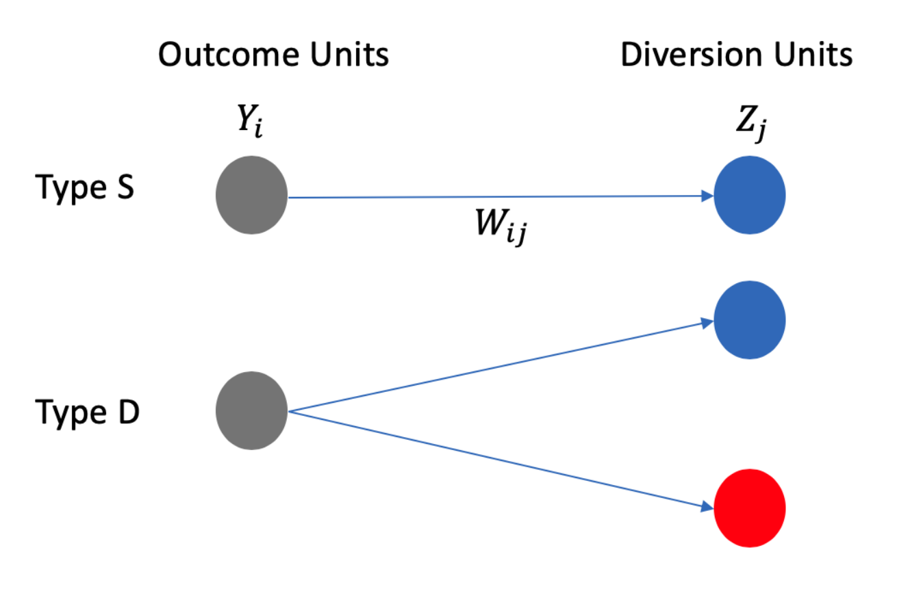
Suppose we are given a simple bipartite graph with two types of outcome units: outcome units of type (single) are connected to a single diversion unit and outcome units of type (double) are connected to exactly two diversion units, such that each outcome unit is connected to its own set of diversion units, each diversion unit being connected to a single outcome unit. To simplify the exposition further, we will assume that the graph weights of outcome units of type (resp. ) are equal to (resp. ), such that the weights corresponding to a given outcome unit always sum to one, and that the two types are present in equal proportions in the graph. Finally, suppose that only units of type react to treatment. Namely, for units of type and for units of type . An illustration is included in Figure 2.
Assuming a treatment assignment sampled uniformly at random with probability , units of type can receive two levels of exposure with equal probabilities ( or with probability ), while units of type can receive three ( or with equal probabilities or with probability ). The first estimator estimates correctly since , but estimates incorrectly since . The discrepancy occurs because units at exposure level are twice more likely to be of type than and not react to treatment, despite both types being equally present in the population. The regression estimator is also biased since . The fact that these two methods produce identical estimates is purely a coincidence. Their estimates will generally be different since the regression approach accounts for outcome values at all observed levels of exposure while the nonparametric approach depends on and only.
3 Unbiased Estimation: Theory
To produce correct estimates in the example of the previous section, we need to account for the fact that not all outcome units have the same exposure distribution. In this section, we introduce estimators of causal effects, inspired by the generalization of the propensity score to the multivalued and continuous treatment literature (Imbens 2000; Hirano and Imbens 2004; Imai and Van Dyk 2004) as well as the literature on estimation under interference (Aronow et al. 2017; Sävje 2019), and prove their unbiasedness under a restricted set of assumptions. We begin with a set of standard assumptions required for our results to hold.
Assumption 1 (Fixed Weights).
The graph weights are not affected by the treatment assignment . Formally, the vector of the treatment assignments is independent of all the weights
For example, in Papadogeorgou et al. 2019, the bipartite graph is given by the fixed geographic distance between power plants and hospitals and is not be affected by the treatment. In the market setting of Pouget-Abadie et al. 2019, the bipartite graph is given by buyers’ preferences for different item categories. It is, of course, in principle possible for items to become more or less desirable to a buyer as a function of treatment. Assumption 1 restricts our attention to the settings where the graph weights are not affected by the treatment.
Assumption 2 (Strong Unconfoundedness).
The exposure received by outcome unit is independent of all its potential outcomes given the graph weights , where : .
Under strong unconfoundedness, the observed exposure of each outcome unit is independent of the potential outcomes of that unit, when conditioned on the bipartite graph weights. Assumption 2 is often compared with its slightly weaker version Imbens 2000.
Assumption 3 (Weak Unconfoundedness).
The assignment to a particular level of exposure is independent of the potential outcome corresponding to that exposure, given the graph weights : , where is the indicator function for outcome unit receiving exposure level .
In practice, while the slightly weaker Assumption 3 is sufficient to establish most of our results, it may be difficult—as argued by Imbens 2000—to find examples where one assumption holds while the other does not, and it may be easier to reason about the more intuitive Assumption 2 directly. In the case of the linear treatment exposure assumption made in Pouget-Abadie et al. 2019, both Assumption 2 and Assumption 3 are verified for Bernoulli or Completely Randomized treatment assignments. Indeed, conditionally on , the exposure received by outcome unit is a fixed weighted-sum of random variables orthogonal to the potential outcomes of unit .
3.1 The Generalized Propensity Score
We now introduce our suggested generalized-propensity-score-based estimator, inspired by the extension of the propensity score to the multivalued and continuous treatment literature (Hirano and Imbens 2004) .
Definition (Generalized Propensity Score).
Let the Generalized Propensity Score for exposure level and weights be the probability of receiving exposure conditionally on the weights : .
In the spirit of early results by Rosenbaum and Rubin 1983, under weak unconfoundedness, it is sufficient to condition on the generalized propensity score to get conditional independence of and . Formally, this result is summarized in the following two lemmas.
Lemma 2 follows mainly from Lemma 1, and is key to setting up the unbiasedness result of our estimator. It states that to achieve independence between the potential outcome corresponding to exposure with the event of receiving that same exposure level, it suffices to condition on the propensity score at that same exposure level. This saves us from having to condition on the entire vector , and observing little to no outcomes at a given conditioned exposure level. We now present the main theoretical result allowing for unbiased estimation of the exposure-response function, and its derived estimands.
Theorem 1.
The proofs of Lemmas 1, 2, and Theorem 1 closely follow those in Imbens 2000 and can be found in the Appendix.
We can also formulate a result for a Horvitz-Thompson-style estimator in the spirit of Horvitz and Thompson 1952.
Theorem 2.
Under the Fixed Weights assumption and the Weak Unconfoundedness assumption, for each such that for all :
where .
This theorem is proven in the Appendix.
Note that under the linear exposure assumption in a simple randomized design, where each with some probability independently of , the property for all is satisfied for and , but may not hold for any other value of .
3.2 Revisiting the Simple Example
We illustrate the merit of the generalized propensity score estimator on the simple example from Section 2. We begin by computing the average of potential outcomes at all levels of exposure and propensity score, .
To estimate the exposure response curve at and , we compute the average of at and , making sure to use the propensity score of each outcome unit for the imputed exposure level, as opposed to the propensity score for their observed exposure level. Units of type (resp. type ) have the propensity score of (resp. ) at the exposure levels , leading to since each type is present in equal proportions. It follows that is equal to if and if , in line with the true exposure response function .
To illustrate the statement of Theorem 2 let us consider, for example, .
For units of type , implies that and . In the overall population units of type with represent half of all type units or a quarter of all units. For units of type , implies that , and these units represent one quarter of all type units or one-eighth of all units in the population. For any unit with its contribution to the expectation in the right-hand-side of the equation in Theorem 2 is zero.
As a result, we estimate as which is indeed the case.
4 Practical Considerations for Unbiased Estimation
Provably unbiased estimates of the exposure-response function can only be obtained at exposure levels which every outcome unit has a positive probability of receiving. Depending on the nature of the bipartite graph, the weights assigned to the edges, and the treatment assignment design, this may eliminate from consideration most if not all exposure levels. Thankfully, practitioners generally assume some form of regularity for the potential outcomes. Bucketing exposure levels to an appropriate granularity allows us to faithfully represent the exposure response curve while ensuring that each outcome unit can effectively receive an exposure within every exposure bucket with some positive probability. To compute the probability of an outcome unit receiving an exposure level within a given bucket, it may be easier to do so by simulating a sufficient number of treatment assignments and computing a histogram approximation of each outcome unit’s exposure distribution.
Furthermore, while the generalized propensity score methodology begins by estimating the exposure-level-cross-propensity-score function , doing so nonparametrically may be difficult if the data is too sparse to obtain meaningful estimates, even when bucketing exposure levels and propensity scores as suggested in the previous paragraph. Practitioners may find more success with a parametric form for . In their paper on propensity scores for the continuous treatment case, Hirano and Imbens 2004 suggest using a second degree polynomial of the exposure, , and the generalized propensity score, . This amounts to running a regression of on a constant, , , , , and the interaction term, , and using the resulting approximation in the second step of the unbiased estimation methodology: . Another alternative is to use a flexible machine learning approach that can capture the nonlinearity of . In Section 6, we present results based on using kernel ridge regression (Friedman et al. 2001, see, for example,).
Moreover, while our estimator is provably unbiased under a standard set of assumptions, it may suffer from having large variance in practice, a common problem of propensity-score-based methods. One suggestion is to impute the exposure response curve at many different levels of exposure, and fit a parametric form to “smooth out” the imputed curve. For example, under the linear exposure assumption with normalized weights considered in Pouget-Abadie et al. 2019, as the number of outgoing edges of an outcome unit grows, the variance of its received exposure shrinks towards its expectation , leaving the experimenter with few observations at exposures .
Finally, an alternative to the suggested generalized-propensity-score-based estimator is to stratify using characteristics of each unit’s exposure distribution (e.g. some moments of that distribution). Such a stratified estimator would compute the average observed outcomes for all units receiving a given exposure coupled with having those characteristics within a certain range. The estimates from each strata would then be pooled together to estimate the exposure response function. A similar method was suggested by Imai and Van Dyk 2004 for the continuous treatment case of classically-run randomized experiments. While it is not guaranteed to produce unbiased estimates, this method may be easier to compute than generalized propensity scores and in some cases still reduces the bias compared to more naïve estimators.
4.1 Additional Considerations for Observational Data
While we are primarily concerned with experimental settings, the results of Section 3 are formulated in a way that makes them valid in observational settings as long as the unconfoundedness assumptions are satisfied. In practical terms, working with observational data usually implies two things:
- •
The functional form of the generalized propensity scores is unknown and the generalized propensity scores must be estimated.
- •
There is a variety of potential estimands of interest.
The first point is self-explanatory and expanded on in Section 6.3, but the second point merits discussion. In many experimental settings, the researchers are primarily interested in estimating , the average effect of treating the whole population versus not treating anyone. When dealing with observational data, treating the whole population may not be feasible and the researchers might be interested in evaluating the cost-effectiveness of a marginal intervention which is the case in, for example, Papadogeorgou et al. 2019.
5 Variance Estimation
The proposed approach can be considered practical only if it provides a way to estimate confidence intervals for the parameter of interest. One simple way to estimate variance is to treat the model as a simple regression problem, ignoring the dependence of exposures across outcome units. For example, the “naïve bootstrap” method would sample individual observations with replacement, computing for each sample set a value for the estimator and constructing the confidence interval using the quantiles of the resulting distribution.
We begin by showing that these standard variance estimators lead to correct coverage probabilities under a general potential outcomes model with error terms:
| (1) |
where is a parametric function of the graph weights and exposure , subject to certain regularity conditions, and are vectors of dimensions and respectively, and the error term verifies and , where is the identity matrix. We refer the reader to the Appendix for the proof of the following theorem and a discussion of the regularity conditions on .
Theorem 3.
Under the response model of Equation 1, both the naïve bootstrap- and the asymptotic OLS-based methods lead to valid confidence intervals.
The assumption of uncorrelated error terms may not be tenable in many cases. In the context of market experiments discussed in the introduction, a seller may change the price of an item affecting the total amount spent by every buyer that buys from that seller. To capture these correlated error terms, we consider a more general model:
| (2) |
where the correlation is introduced through the additional term. Let , such that the response model can be more concisely written as . To avoid identification issues for , we impose that are normal, with mean and variance .
Theorem 4.
Under some regularity assumptions on (discussed in the Appendix) and the response model of Equation 2, we have:
where and . Furthermore, the naive bootstrap estimator results in a sample average of .
Theorem 4 states that the naïve bootstrap estimator will not produce correct confidence intervals in general. A proof is given in the Appendix. To construct valid confidence intervals, we need to correctly specify and estimate both and properly. We suggest the following parametric bootstrap procedure:
Assuming that outcomes follow the structural form of Equation 2, the parametric bootstrap method in Algorithm 1 recovers the correct distribution of its parameters, which is formalized in the following theorem:
Theorem 5.
A proof is included in the Appendix. We validate this method empirically in Section 6.1.
6 Empirical Results
Through simulation on synthetic graphs as well as the Amazon buyer-item graph from Pouget-Abadie et al. 2019, we show that our suggested estimators and bootstrap variance estimation methods outperform the naïve approaches. We also apply the proposed methodology to the observational dataset from Zigler and Papadogeorgou 2018 and discuss the results.
6.1 Fully Simulated Example
We begin by comparing 3 estimation procedures on a completely simulated dataset:
- (i)
a “naïve regression” of on without consideration of the heterogeneous exposure distributions across outcome units,
- (ii)
a parametric model for a correctly specified (assumed known) functional form of ,
- (iii)
a non-parametric propensity-score-based approach utilizing kernel ridge regression that is agnostic to the exact functional form of .
Our simulated bipartite graph consists of outcome units and diversion units. Each outcome unit is connected to diversion units, where is distributed uniformly over the set of integers from to . All weights are set to be equal to . For the diversion units, the treatment assignments are chosen to be Bernoulli random variables with parameter . We start by letting and from Section 5, which implies uncorrelated errors.
We consider two forms for the exposure-response function. Under the first specification, we let , where in order to make each specification more comparable to the other. We refer to this exposure-response specification as having homogeneous treatment effects. In this case, the naïve regression method (i) coincides with the correctly specified model (ii), thus we report only the results for the former in Table 1. Under the second specification, we let : the more diversion units a given outcome unit is connected to, the stronger it reacts to small changes in exposure—in other words, we have heterogeneous treatment effects across outcome units.
We run simulations and compare the methods based on the average bias as well as the average Root Mean Square Error (RMSE) of the estimates , where the average is taken across the simulations. We construct nominally 95% confidence intervals using naïve bootstrap samples, as suggested by Theorem 3 of Section 5. Table 1 reports the results. Reductions in bias and RMSE relative to the naïve approach are reported alongside the absolute numbers. As expected, naïve regression only performs well for homogeneous treatment effects, while correctly-specified models for always perform well. Non-parametric approaches like kernel ridge regression that approximate outperform the naïve approach across both settings.
Furthermore, we find that naïve bootstrap coverage is correct for all properly-specified models ((i) and (ii) for homogeneous treatment effects, and (ii) only for heterogeneous treatment effects), validating the results of Theorem 3. While we have no explicit guarantees for the coverage of the naïve bootstrap for kernel-ridge regression, we find that it performs well for homogeneous treatment effects, and outperforms the naïve regression for heterogeneous effects.
| Fully Simulated Data | Amazon Graph | |||||
| Method | (i) | (ii) | (iii) | (i) | (ii) | (iii) |
| Homogeneous treatment effects | ||||||
| Bias of | ||||||
| Bias reduction | ||||||
| RMSE of | ||||||
| RMSE reduction | ||||||
| Naïve Bootstrap Coverage | ||||||
| Heterogeneous treatment effects | ||||||
| Bias of | ||||||
| Bias reduction | ||||||
| RMSE of | ||||||
| RMSE reduction | ||||||
| Naïve Bootstrap Coverage | ||||||
Notes: (i) naïve regression, (ii) correctly specified parametric model, (iii) kernel ridge regression
Correlated Errors.
We ran another set of simulations allowing correlated errors and setting . We consider the case of homogeneous treatment effects and compare the naïve bootstrap against the parametric bootstrap approach proposed in Section 5. We assume that the functional form of is known as discussed in that section and show that the parametric approach achieves the coverage of , while the naïve approach achieves only coverage, validating the claim made in Theorem 5.
6.2 Amazon Data
We repeat the analysis from the previous section using a sub-sample of the user-item graph based on Amazon reviews from He and McAuley 2016; McAuley et al. 2015. The graph structure in this example is obtained by sampling users with the numbers of reviews ranging from just a few to several dozen. The rest of the data generating process remains unchanged relative to the fully simulated dataset. The results based on simulations are reported in Table 1 and lead to the same conclusions as we obtained from the fully synthetic graph.
6.3 The Hospital-Power Plant Dataset Papadogeorgou et al. 2019
The authors of (Papadogeorgou et al. 2019) analyze a real-world setting whereby a specific filter system is implemented at certain power plants across the US and they seek to determine its impact on cardiovascular disease (CVD) hospitalization rates in the surrounding areas. In total, there are power plants playing the role of the diversion units, and zipcodes, playing the role of the outcome units, included in the study, which ran from June to August in 2004.
The response of the outcome units is measured in the number of hospitalizations for CVD among certain medicare beneficiaries. Due to the sensitivity of these data, we use the simulated outcome data provided by the authors of Papadogeorgou et al. 2019. All other covariates were provided as is.
There are a few notable differences between this and the two other settings discussed in the current section. Most importantly, Papadogeorgou et al. 2019 deals with observational data. Consequently, the unconfoundedness assumptions are not trivially satisfied and have to be justified based on the available data and institutional knowledge of the researchers. Another important feature is that the functional forms of neither the propensity score function, nor the exposure response function are known to the researchers. This implies that the propensity score function has to be estimated from data and that—unlike in the two previous examples—we cannot compare the performance of the proposed method to that of the correctly specified model since the correct specification is unknown. In essence, there is no “ground truth” to use for evaluation. It is, however, still possible to compare the estimates obtained using the naïve approach and the proposed methodology. If these estimates are substantially different from each other, the researchers might want to put additional effort into investigating the potential reasons behind such a discrepancy. The main reason we present these results is to illustrate how the methods we propose can be used in purely observational settings.
To define the bipartite graph, we use the same grouping method as the one implemented in the original paper. We construct geographic clusters and assume that zipcodes within each cluster are only affected by the power plants belonging to that same cluster (see the source paper for an illustration). If a zipcode and a power plant find themselves in the same cluster, we create a bipartite edge with the weight inversely proportional to the geographic distance between them (and so that all the weights still add up to one). In our simulations we employ the linear exposure assumption from Pouget-Abadie et al. 2019, such that, for a given outcome unit , , where signifies that power plant has installed the filter and the weights are normalized and inversely proportional to the distance from zipcode to power plant .
In Papadogeorgou et al. 2019 the authors do not assume an identically distributed assignment to treatment for each power plant. They fit a diversion-unit-level propensity score model to learn at which rate each power plant receives the treatment. We use similar methodology and predict the treatment status utilizing a linear SVM and the power plant level features.
Given that the outcome data provided by the authors is obscured for sensitivity reasons, no direct comparison of our estimates to those presented in Papadogeorgou et al. 2019 is informative. For this reason, we employ the linear exposure assumption which may not be the most adequate exposure mapping assumption in this setting. It, however, allows us to maintain the methodology from the rest of this paper.
Our main estimand of interest is the average treatment effect between the exposures and . To be able to estimate this treatment effect we need to predict the probabilities of observing these exposure levels for each outcome unit. We assume that each power plant is treated independently with the probability estimated using the linear SVM model described above. This allows us to construct the exposure distribution. Namely, with all weights having distinct values across , the probability of observing is estimated as:
where is the estimated probability that .
We estimate the exposure response by utilizing the naïve regression and the kernel ridge method outlined in Section 6.1. We also present the 95% confidence intervals produced using bootstrap simulations.
| Method | (i) | (ii) |
|---|---|---|
| Average Treatment Effect | ||
| 95% Confidence Intervals |
Notes: (i) naïve regression, (ii) kernel ridge regression
The estimates from the two methods are neither significantly different from zero, nor from each other. However, the confidence intervals produced using the kernel ridge method are almost 40% tighter.
7 Conclusion
We have shown that practitioners that use bipartite designs should be conscious of the possible bias concerns of inference methods that do not account for heterogeneous treatment effects and exposure distributions. We suggest propensity score corrections inspired largely by the work from Hirano and Imbens 2004 and Imai and Van Dyk 2004, and discuss practical considerations when using such estimators. We provide new theoretical results showing that naïve bootstrap methods lead to correct coverage probabilities for response models with uncorrelated errors, and suggest a parametric bootstrap method for a set of response models with correlated error terms. Our theoretical results are validated on synthetic and real-world graphs through simulations. We also consider an observational setting and compare the results obtained using the naïve and the proposed approaches. Potential future research directions include a more thorough investigation of estimation and inference methods which tackle experiments that might affect the structure of the bipartite graph.
References
- Aronow et al. (2017) Aronow, P. M., C. Samii, et al. (2017). Estimating average causal effects under general interference, with application to a social network experiment. The Annals of Applied Statistics 11(4), 1912–1947.
- Del Prete et al. (2020) Del Prete, D., L. Forastiere, and V. L. Sciabolazza (2020). Causal inference on networks under continuous treatment interference. arXiv preprint arXiv:2004.13459.
- Eckles et al. (2017) Eckles, D., B. Karrer, and J. Ugander (2017). Design and analysis of experiments in networks: Reducing bias from interference. Journal of Causal Inference 5(1).
- Fatemi and Zheleva (2020) Fatemi, Z. and E. Zheleva (2020). Minimizing interference and selection bias in network experiment design. arXiv preprint arXiv:2004.07225.
- Forastiere et al. (2016) Forastiere, L., E. M. Airoldi, and F. Mealli (2016). Identification and estimation of treatment and interference effects in observational studies on networks. arXiv preprint arXiv:1609.06245.
- Friedman et al. (2001) Friedman, J., T. Hastie, and R. Tibshirani (2001). The elements of statistical learning, Volume 1. Springer series in statistics New York.
- Galagate (2016) Galagate, D. (2016). Causal inference with a continuous treatment and outcome: alternative estimators for parametric dose-response functions with applications. Ph. D. thesis.
- He and McAuley (2016) He, R. and J. McAuley (2016). Ups and downs: Modeling the visual evolution of fashion trends with one-class collaborative filtering. In proceedings of the 25th international conference on world wide web, pp. 507–517.
- Hirano and Imbens (2004) Hirano, K. and G. W. Imbens (2004). The propensity score with continuous treatments. Applied Bayesian modeling and causal inference from incomplete-data perspectives 226164, 73–84.
- Holtz et al. (2020) Holtz, D., R. Lobel, I. Liskovich, and S. Aral (2020). Reducing interference in online marketplace pricing experiments. Available at SSRN.
- Hong and Raudenbush (2005) Hong, G. and S. W. Raudenbush (2005). Effects of kindergarten retention policy on children’s cognitive growth in reading and mathematics. Educational evaluation and policy analysis 27(3), 205–224.
- Horvitz and Thompson (1952) Horvitz, D. G. and D. J. Thompson (1952). A generalization of sampling without replacement from a finite universe. Journal of the American statistical Association 47(260), 663–685.
- Hudgens and Halloran (2008) Hudgens, M. G. and M. E. Halloran (2008). Toward causal inference with interference. Journal of the American Statistical Association 103(482), 832–842.
- Imai and Van Dyk (2004) Imai, K. and D. A. Van Dyk (2004). Causal inference with general treatment regimes: Generalizing the propensity score. Journal of the American Statistical Association 99(467), 854–866.
- Imbens (2000) Imbens, G. W. (2000). The role of the propensity score in estimating dose-response functions. Biometrika 87(3), 706–710.
- Johari et al. (2020) Johari, R., H. Li, and G. Weintraub (2020). Experiment design in two-sided platforms: An analysis of bias. Submitted.
- Kempton (1997) Kempton, R. (1997). Interference between plots. In Statistical methods for plant variety evaluation, pp. 101–116. Springer.
- McAuley et al. (2015) McAuley, J., C. Targett, Q. Shi, and A. Van Den Hengel (2015). Image-based recommendations on styles and substitutes. In Proceedings of the 38th International ACM SIGIR Conference on Research and Development in Information Retrieval, pp. 43–52.
- Ogburn et al. (2017) Ogburn, E. L., O. Sofrygin, I. Diaz, and M. J. van der Laan (2017). Causal inference for social network data. arXiv preprint arXiv:1705.08527.
- Papadogeorgou et al. (2019) Papadogeorgou, G., C. Choirat, and C. M. Zigler (2019). Adjusting for unmeasured spatial confounding with distance adjusted propensity score matching. Biostatistics 20(2), 256–272.
- Pouget-Abadie et al. (2019) Pouget-Abadie, J., K. Aydin, W. Schudy, K. Brodersen, and V. Mirrokni (2019). Variance reduction in bipartite experiments through correlation clustering. In Advances in Neural Information Processing Systems, pp. 13288–13298.
- Rosenbaum and Rubin (1983) Rosenbaum, P. R. and D. B. Rubin (1983). The central role of the propensity score in observational studies for causal effects. Biometrika 70(1), 41–55.
- Rubin (1980) Rubin, D. B. (1980). Randomization analysis of experimental data: The fisher randomization test comment. Journal of the American statistical association 75(371), 591–593.
- Saint-Jacques et al. (2019) Saint-Jacques, G., J. E. Sorenson, N. Chen, and Y. Xu (2019). A method for measuring network effects of one-to-one communication features in online a/b tests. arXiv preprint arXiv:1903.08766.
- Saveski et al. (2017) Saveski, M., J. Pouget-Abadie, G. Saint-Jacques, W. Duan, S. Ghosh, Y. Xu, and E. M. Airoldi (2017). Detecting network effects: Randomizing over randomized experiments. In Proceedings of the 23rd ACM SIGKDD international conference on knowledge discovery and data mining, pp. 1027–1035. ACM.
- Sävje (2019) Sävje, F. (2019). Causal inference with misspecified exposure mappings. Technical report, Technical report, Technical report, Yale University.
- Struchiner et al. (1990) Struchiner, C. J., M. E. Halloran, J. M. Robins, and A. Spielman (1990). The behaviour of common measures of association used to assess a vaccination programme under complex disease transmission patterns—a computer simulation study of malaria vaccines. International journal of epidemiology 19(1), 187–196.
- Tchetgen and VanderWeele (2012) Tchetgen, E. J. T. and T. J. VanderWeele (2012). On causal inference in the presence of interference. Statistical methods in medical research 21(1), 55–75.
- Toulis and Kao (2013) Toulis, P. and E. Kao (2013). Estimation of causal peer influence effects. ICML, 1489–1497.
- Viviano (2020) Viviano, D. (2020). Experimental design under network interference. arXiv preprint arXiv:2003.08421.
- Zigler and Papadogeorgou (2018) Zigler, C. M. and G. Papadogeorgou (2018). Bipartite causal inference with interference. arXiv preprint arXiv:1807.08660.
Appendix A Additional Results
A.1 Additional Sufficient Conditions for the Unbiasedness of Naïve Estimators
We present two results that provide—rather strong—sufficient conditions for the unbiasedness of naïve estimators.
In other words, if potential outcomes are the same in expectation regardless of the graph weights, then averaging the outcomes observed at a given exposure level produces an unbiased point estimate of the exposure-response curve.
If, in addition to the assumptions in Proposition 1, and strong unconfoundedness holds, the naïve regression produces an unbiased estimate too.
A.2 Details on Unbiased Estimator with Proper Coverage
Assume that we are interested at finding at a finite number of potential exposures . Let
and . Then the regression coefficient in front of from the regression of on is given by the expression:
As , by LLN:
which is equal to .
Hence, , which was shown to be an unbiased and consistent estimator of . Theorem 3 can then be used for constructing confidence intervals around .
A.3 Block Design
An alternative to the parametric bootstrap approach discussed in the paper is a block (or cluster) design inspired by the time series literature. The idea is to split the graph into several components and perform a bootstrap procedure by sampling the entire components instead of individual observations. This allows to preserve the correlation structure within each component. In this section we present some theoretical properties and discuss simulation results utilizing this approach.
The graph is generated as follows. First, a number of blocks, , are drawn from distribution over blocks characterized by the measure . Then a number of weak links for is drawn. The weakness means that is small (exact technical conditions to be worked out).
Recall that , where the total number of outcome units and and are sub-vectors of regressors (exposures and unit vector) and residuals respectively. The variance of the estimator is then:11 1 Should be inverse matrices instead of division, please read accordingly.
where and the number of outcome units in block . Next, as the terms in the sum are independent, we have:
All objects in those expressions can be estimated by sample analogues. Indeed, the denominator can be directly approximated as , while the numerator becomes . The last expression can further be simplified under different assumptions.
To illustrate the ideas presented in this section we perform simulations on a bipartite graph that can be split into components. There may or may not be some edges connecting different components. We illustrate (see Figure 3) the performance of the clustered bootstrap by plotting the coverage of the proposed method in comparison with the naïve bootstrap approach as a function of the share of total graph edges cut by separating the graph into disjoint components. The more edges are cut, the worse is the performance of the clustered approach. However, it can be a good alternative to the naïve design, when there are not too many edges connecting different components. In practice, the researcher will have to determine the suitable components using one of the graph clustering algorithms. The comparison of different alternatives while important, is beyond the scope of this paper.
A.4 Formal Construction of the Data Generating Process for Variance Estimation with Examples
In this section, we detail a formal construction of the data generating process that is used to prove the results of Section 5, namely Theorems 3 and 3.
Each outcome unit’s outcome is considered as a realized sequence of , where the set of possible sequences is denoted as and
- •
is a vector of length of unobserved shocks (errors).
- •
is a sequence of graphs with arbitrary number of divergence units and outcome units
- •
are the corresponding weights of the graph
- •
is realizations of treatments over divergence units of graph .
There is a sequence of underlying -algebras over with the property that is measurable with respect to . are the measures over those -algebras. Note that , , and uniquely define the exposure generating process . A few examples below show how this formal construction can be applied rigorously.
- •
Standard treatment effects. In this case is a bipartite graph of diversion units and outcome units with unweighted edges. are the iid random variables drawn from a distribution with mean 0 and finite . is the product -algebra, and is the product measure. .
- •
Weakly dependent blocks. is now a graph of blocks, with edges between each pair of blocks. denote the weights of the inner links and between-links, with the property that the ratio of between-weights to within-weights converges to 0 a.s. In this example, are the iid random variables drawn from a distribution with mean 0 and finite . is the product -algebra, and is the joint distribution satisfying the property that marginal distribution of observing a particular set of blocks (i.e., integrating out ) results in the product measure over blocks. .
- •
Influential units. For this specific setting, we consider non-trivial -algebras. For example, the graph contains a single influential unit, with all other units being like the standard treatment effects example. In that case, we have , indicating events of the influential unit being treated or not. The rest of the construction is the same like in standard treatment example with the exception that -algebras and measures now have to be cross-producted with and the measure over respectively. Note that in this construction we have for any :
even though all units have independent realizations of u’s and Z’s.
- •
AR-1 process. Suppose that enumerates both types of units and the link between an outcome and diversion units exists iff the number of outcome unit is equal to the number of diversion unit or greater than that number by exactly one. In this scenario, the path-based distance between any two outcome units and is equal to . Setting results in the AR-1 process.
- •
Clusters. Diversion units are a union of two subsets and . Each of the outcome units is connected to one unit in and one unit in . .
Appendix B Proofs
B.1 Proof of Proposition 1
Note: In this proof as well as the next one, we slightly abuse the notation by using to refer to all of the graph weights, not just those corresponding to outcome unit .
As if and only if , we can write
where the second to last equality follows from weak unconfoundedness and the last equality follows from .∎
B.2 Proof of Proposition 2
For the naïve regression estimator we have
where
The second and third equalities follow from the fact that for all and strong unconfoundedness.
Consequently, ∎
B.3 Proof of Lemma 1
Since, by definition, , we have:
Next,
since and taking into account the equality above. As a result,
Hence, and are independent conditional on .∎
B.4 Proof of Lemma 2
Similarly to the previous proof,
where the second equality follows from the weak unconfoundedness. Since we also know from the previous lemma that , we have:
and, as a result, and are independent conditional on .∎
B.5 Proof of Theorem 1
Let’s prove the first equality.
Therefore, using weak unconfoundedness,
which proves the first equality.
For the second equality we have:
where the second equality follows from the law of iterated expectations.∎
B.6 Proof of Theorem 2
First, by the law of iterated expectations
which is equal to
since
Next, given , we have and . Therefore, the expression above conditional on , can be written as:
As is a function of and is independent of conditional on (weak uncondoundedness), we can remove the conditioning on . The expression becomes:
where we use the definition of the generalized propensity score to replace by .∎
B.7 Proof of Theorem 3
Assumption 4.
The cumulative distribution function of produced by the Data Generating Process (DGP) converges almost surely to , where is -measurable.
Conditional on any realization of the data, we can write:
By Assumption 1, the first term converges a.s. to some and the second term converges in distribution to .22 2 Independence of ’s imply that only the products of with survive in the variance term. As a consequence, .
Let us calculate the asymptotic intervals for naive bootstrap and naive normal approximation. Standard reasoning implies that conditional on both procedures asymptotically approximate as , which is exactly the same form, as the correct distribution. Hence, in the limit we have for almost any .
It then follows that:
∎
B.8 Proof of Theorem 4
In this case, we can denote and see that:33 3 There is clearly a problem with this expression as can require enormous computational power. That’s why we need to impose approximate block structure and use bootstrap for practical applications. However, for smaller applications we do not even need any of those assumptions.
As a result, is an unbiased estimator of conditional on any realization of . Consequently:
To prove asymptotic distribution results, we would need an extra assumption on the behavior of the interplay between and of the following form:
Assumption 5.
with being -measurable.
Recall that under Assumption 4, . The variance of is given by the expression:
B.9 Proof of Theorem 5
From Theorem 4 it follows that:
which is equal to asymptotically as soon as and are consistent. We now show that they are. Since are uniformly consistent estimates for as long as is consistent, converge uniformly to –the residuals from regression of true on . Denote and the projection and residual from projection on respectively. Note that both these matrices are symmetric meaning that and idempotent meaning that . Finally, as , . Hence:
The first term converges almost surely to , while the second term is a random variable with the variance equal to:
As , . Finally, as , is also consistent.