Curve valuations and mixed volumes in the implicitization of rational varietiesThanks: MIH and AD were supported by ANPCyT PICT 2016-0398, Argentina. AD was also partially supported by UBACYT 20020170100048BA, CONICET PIP 11220150100473, Argentina.
Abstract.
We address the description of the tropicalization of families of rational varieties under parametrizations with prescribed support, via curve valuations. We recover and extend results by Sturmfels, Tevelev and Yu for generic coefficients, considering rational parametrizations with non-trivial denominator. The advantage of our point of view is that it can be generalized to deal with non-generic parametrizations. We provide a detailed analysis of the degree of the closed image, based on combinatorial conditions on the relative positions of the supports of the polynomials defining the parametrization. We obtain a new formula and finer bounds on the degree, when the supports of the polynomials are different. We also present a new formula and bounds for the order at the origin in case the closed image is a hypersurface.
Key words and phrases:
implicitization, Newton polytope, tropical geometry, generalized Puiseux series2010 Mathematics Subject Classification
14M25, 14T05, 68W301. Introduction
A classical question that has thrived research in Computational Algebraic Geometry is the problem of implicitization. The aim is to describe the prime ideal of polynomial relations among the coordinates of a rational map . We concentrate on sparse elimination and we consider a family of rational maps of the following form: the input is a field of characteristic zero, finite sets of lattice points in and non-zero Laurent polynomials in variables supported on these sets. More precisely,
| (1.1) |
and our parametrization is of the form
| (1.2) |
As the ideal of relations among the coordinates of is defined over any subfield containing the coefficients, we will assume in what follows without loss of generality that is algebraically closed. We can think of the implicitization problem as a moduli question, as the answer differs depending on the genericity of the coefficients . We will consider with the trivial valuation. In [19], Sturmfels, Tevelev and Yu approached this question with tools of tropical geometry, thus exploiting the combinatorial nature of the problem. Instead of finding the ideal of relations, we can compute its tropicalization. This is a rational weighted balanced polyhedral fan in that captures the combinatorics of this ideal. Tropical implicitization techniques are well suited to study the generic points of this space via the theory of Geometric Tropicalization developed by Hacking, Keel and Tevelev [4, 11]. These techniques are hard to address for special choices of coefficients, since they depend on the process of resolution of singularities.
We approach this question from a different perspective. Namely, we go back to the valuative approach to tropical geometry, manifested in the Fundamental Theorem of Tropical Geometry [6, 7], and we reinterpret tropical implicitization in this elementary language. The main advantage of this approach is that we recover in Theorem 2.5 a straightforward generalization of the description of [19, Theorem 2.1] for generic parametrizations, while developing tools that could be further refined to study the non-generic case. In fact, Theorem 2.5 can be deduced from their result, as we discuss in Section 2.6.
We also study in detail the degree of the closed image of (that is, the closure of the image of ) which we denote by , in case it has dimension . When is a hypersurface (that is, when ), one can get the direction and the length of the edges of the Newton polytope of a defining equation for from the description of the cones in the tropicalization of the image of and their multiplicities Then, can be algorithmically reconstructed, see for instance [13]. We could then from this information extract the degree . In the case of lattice polygons, there is a clear description of in [5]. If and all supports are equal, is computed in [20] by means of resultants. In case is a monomial, the description of the Newton polytope of was also studied in general by Esterov and Khovanskii in [9], where they develop an elimination theory of polytopes via mixed fiber polytopes in the sense of McMullen. This gives the Newton polytope only for generic coefficients, from which can be read in this case. We give a precise description in Theorem 3.3.
There is a straightforward upper bound for , given by the lattice volume of the convex hull of the union of the supports (see for instance [8] in case ). The divergence from this upper bound for generic coefficients is related to the following question. Given and Laurent polynomials in variables with these supports respectively and generic coefficients, when generic linear combinations with generic coefficients , have generic coefficients with respect to the support ? In Theorem 3.3 we give conditions on the relative positions of under which this upper bound and some refined ones are attained. The conditions are similar to the conditions of monotonicity of the mixed volume studied in [2] for the case of sparse polynomials in variables, but they are in fact different as Example 3.8 shows.
When is a hypersurface, we also compute by means of curve valuations the order at the origin . Again, if the Newton polytope is known, this information can be extracted from it. Under our hypotheses, the origin is never in the image of , but it could be in its closure. We compute in Theorem 4.2 under a condition on the family of supports that holds in many cases. This order can be greater than one (that is, the origin is a singular point of the closure of in ) even for generic coefficients, depending again on the relative positions of the supports . We also give along the paper examples not satisfying the hypotheses of our results, but were we can still compute degree and order adapting the arguments in our proofs.
In Section 2 we describe the tropicalization of . We prove the basic Theorem 2.1 and the main Theorem 2.5. We also show in § 2.5 how this result and its proof can be used in generic and non-generic cases. Section 3 deals with the degree computation for any . Our main result there is Theorem 3.3 and in § 3.1 we give different conditions for equality in the inequalities in its statement, in case . Section 4 deals with the computation of the order of at the origin for . We present our main result Theorem 4.2 and we discuss examples that show how its proof can be used to study cases in which the hypotheses are not satisfied.
2. The tropicalization of the image of
We fix a family of finite integer sets and we take Laurent polynomials as in (1.1) with these respective supports and coefficients in . The goal of this section is to describe the tropicalization of the closure of the image of in (1.2) in case the coefficients of are generic. Since the parametrization is invariant under multiplication of all the ’s by the same monomial, that is under a common translation of the supports, we will assume all along, without loss of generality, that our supports lie in the positive orthant , that is, that .
Our main result in this section is Theorem 2.5, which describes the tropicalization of the closure of the image of as a set. It extends [19, Theorem 2.1] to the case of rational functions. Our proof is built from Theorem 2.1 and Lemma 2.7 below using curve valuations. The main advantage of this approach is that it only involves elementary techniques and it hints on how to proceed in case the coefficients fail to be generic. We develop this idea in § 2.5. In Section 2.6 we recover the associated multiplicities from the results in [18].
2.1. Tropical varieties
In this section, we present some basic definitions and notation. In particular, we give an introduction to useful statements on tropical geometry from the valuative perspective and recall the connection between initial ideals, tropicalizations and power series solutions to Laurent polynomial equations. Our main result here is Theorem 2.1.
We start by recalling the definition of the tropical variety of an ideal from the point of view of Gröbner theory. We consider an algebraically closed field of characteristic zero with trivial valuation. As usual, we set and we call the -torus. For any nonzero Laurent polynomial and , we denote by the subsum of those terms in for which and is minimum. We denote by the ideal generated by all the initials with respect to of all nonzero polynomials .
Given an ideal , the support of the associated tropical variety or tropicalization of is the set:
| (2.1) |
Given an algebraic variety , we set , where denotes the ideal of Laurent polynomials vanishing on .
By Hilbert’s Nullstellensatz, records all points such that the associated variety is nonempty. When the ideal is principal, generated by a Laurent polynomial , the set consists of all directions for which the initial form is not a monomial. Thus, consists precisely of the codimension one cones in the inner normal fan of the Newton polytope of , that is, of the convex hull of the exponents of the monomials occuring in with nonzero coefficient.
Tropical geometry can be approached from the perspective of valuations, when we think of them as Bieri-Groves’ sets [3]. To state explicitly the link between the previous definition (2.1) and the characterization of the tropicalization of via curve valuations, we introduce the algebraically closed field of power series with real exponents and well-ordered supports , known as generalized Puiseux series.
An element has the form , where , and is a sum of terms of the form with and for all . We call its initial term and its order. In particular for all . We can extend these notions to tuples in coordinatewise.
The Fundamental Theorem of Tropical Geometry [6, 7] asserts that given an ideal in the Laurent polynomial ring , the tropical variety is the set of all valuations of nonzero generalized Puiseux series solutions to :
| (2.2) |
Note that by choosing the field of generalized Puiseux series which is algebraically closed and complete [16] with value group , it is not necessary to take closure on the right side [15].
The tropicalization is a rational polyhedral set that can be given a (non-unique rational polyhedral) fan structure and any such fan can be refined to a tropical fan structure. The multiplicity of a maximal cone in a fan structure of is defined as the sum over all minimal associated primes of the initial ideal , of the multiplicities:
where is any point in the relative interior of . These multiplicities satisfy a balancing condition. We refer the reader to [18] for details.
Consider now nonzero Laurent polynomials and the map from (1.2). Denote by the extension of to . If is the ideal that defines the variety and , the ideal that defines the variety , then . Given a set , denote by its closure in the Euclidean topology. The next result, which is an easy consequence of (2.2), shows the connection between the tropicalization of the variety parameterized by the rational map and the valuations of points in its image.
Theorem 2.1.
Let be nonzero Laurent polynomials in variables with coefficients in and let be the rational map they define as in (1.2). Then,
| (2.3) |
Proof.
Let . The Fundamental Theorem of Tropical Geometry implies that for every in the preimage of the torus belonging to the domain of . As tropical varieties are closed in the Euclidean topology, we have the inclusion in (2.3). Moreover, since is dense in , we have equality in (2.3) by Theorem A in [3]. Indeed, Bieri-Groves Theorem A asserts that all maximal cones in have dimension equal to . Let be an algebraic variety of codimension such that . Then, all maximal cones in have dimension equal to . Consequently, is dense in , as well as . ∎
2.2. Defining the cones and the statement of Theorem 2.5
We present in Definition 2.4 the cones that occur in the tropicalization of the image of . We first need some notation concerning supports and polytopes. Let be a finite set in and a polynomial with support with for all . For any , we define
| (2.4) |
In particular, if , does not depend on its coefficients and we have
| (2.5) |
as at the beginning of § 2.1.
Let be a lattice polytope and . We will call face the face of which has as an interior normal vector. That is,
| (2.6) |
If is a finite set, (called a face of ) is obtained as the intersection with of the face of the convex hull of defined by . Thus, for any nonzero Laurent polynomial , the Newton polytope of is face.
Given a lattice polytope , we use the notation for its normalized volume with respect to the lattice (so equals times its Euclidean volume ). Given a family of polytopes , we denote by their -dimensional mixed volume
| (2.7) |
If are finite sets, the mixed volume of is defined as the mixed volume of their convex hulls . Recall that, by Bernstein’s Theorem ([1]), this is an upper bound for the number of isolated common zeros in of any system of polynomials with support set . Moreover, equality holds for generic polynomials with those supports.
We denote by the set and by the set .
Definition 2.2.
Given a family of finite sets in (or convex polytopes) and a face of for all , we will say that is a coherent collection of faces of if there exist such that for all .
Definition 2.3.
A family of finite sets in is said to be essential if for any subset of size at most , it holds that
| (2.8) |
With the previous notation, given a set , we will say that a coherent collection of faces of is adapted to if and the family is essential.
Consider again the family of supports . Given any , we define
| (2.9) |
and we consider the map defined by
| (2.10) |
We now define the cones on which the description of is based. We use the notation . Given a subset , we use the standard notation to denote the real vectors satisfying for all and for .
Definition 2.4.
Given a set and a coherent collection of faces of adapted to , we define the following cones in :
- *
if ,
(2.11) - *
if , set and
(2.12)
Note that there is a bijection between faces of , and cones of the inner normal fan of . Denoting by the cone corresponding to a coherent collection of faces of , we have that for every , the cone can be written as as defined by [19], and for ,
We now present Theorem 2.5. Our statements are direct generalizations of [19, Theorem 2.1], but the proofs are different and based on curve valuations and give a hint on how to describe with this tool the tropicalization of the image when the coefficients are not generic.
Theorem 2.5.
Consider the rational map as in (1.2) where have supports and generic coefficients. Then, the following subsets of coincide:
- (i)
the tropical variety ,
- (ii)
the union of the cones , for all such that and all coherent collections of faces of adapted to .
The proof will be given in § 2.4.
Denote by the convex hull of for any . For instance, in the unmixed case when all are dilations of a fixed polytope , that is, when there exists positive integers , such that for all [19, Section 3.2], we have that
The image of varies as in [19] according to whether contains the origin or not. When contains the origin, the image of is and the tropical variety is the union of the cones over all such that , and over all such that . When does not contain the origin, the image of is and is the union of the cones over all such that , and over all such that .
We could use Theorem 2.5 to compute the dimension of the variety parameterized by , which equals the maximal dimension of a cone , because the tropical variety and have the same dimension by [3]. For instance, let . If there exists a subset with and , then parameterizes a hypersurface. Note that the reciprocal is not true. For instance, consider the rational map defined by ,with . Then, parameterizes a hypersurface but for all , in particular those with cardinal . This is not a contradiction because in this case dim
Theorem 2.5 could be seen as a consequence of [19, Theorem 2.1], which applies to the case when is a monomial ( consists of a single point). Consider again finite sets and polynomials with these respective supports such that the closure of the image of the associated rational map has dimension .
Let be the homomorphism of tori with its corresponding linear map of lattices:
| (2.13) |
Denote by the rational map:
| (2.14) |
Then, and thus (see Remark 1.2 in [18]). The cones of the tropical variety can then be deduced from the description of the tropical variety . As we show in Section 2.5, our direct and simple approach via curve valuations can be extended to deal with non-generic parametrizations. Also, curve valuations are used in Section 4 to give a formula for the order at the origin of .
2.3. Two auxiliary results
We first recall Hensel’s lemma. The valuation ring of is , with maximal ideal . Here denotes the units in , i.e. those elements with valuation . Given a sequence of polynomials , let us denote by its associate Jacobian matrix. Observe that the field is algebraically closed, and so a Henselian field. Hensel’s lemma asserts the following (see, for example, [14]). Let be a family of non-zero polynomials. Assume that there exists such that
Then, there exists a unique such that and for all .
The following lemma for polynomials with nonnegative exponents is straightforward.
Lemma 2.6.
Let be a finite set and be a non-zero polynomial supported on . For any with , , , we have
| (2.15) |
Notice that, a priori, we could have so Lemma 2.6 implies that , with equality if and only if .
Lemma 2.7 below gives conditions which ensure that a vector can be realized as the (coordinatewise) valuation of a point in .
Lemma 2.7.
Let be non-zero polynomials in with and call in their respective supports. Given , assume the initial polynomials have a common zero such that their Jacobian matrix has maximal rank . Then,
- (i)
for each verifying that for all , there exist with such that for all .
- (ii)
if have generic coefficients, for each verifying that for all , there exist with such that for all .
Proof.
Write and denote , . By Lemma 2.6, we know that , for all and . Therefore, we can assume that and with for all .
To prove item (i), under these assumptions on and the polynomials , consider the polynomials for every and . By Lemma 2.6, for all . Since and has rank , for any generic affine linear forms that vanish on , the Jacobian matrix of the family of polynomials is invertible when evaluated at . Consider now the Jacobian matrix of the family of polynomials . Since and , . Then, by Hensel’s Lemma there exist such that and for all , and so .
To prove item (ii), note that for a generic point we have for all , thus satisfies the statement. Consider now any . We need to show that there exists a point with and such that for all . Consider the set . Since are generic polynomials and have a common zero , the solution set in is an equidimensional variety of dimension . If we denote by the supports of these initial polynomials, the set with the -th vector of the canonical basis of and when it is repeated times, then the mixed volume is a positive integer. By the monotony of the mixed volume, is also positive. That is, for generic affine linear forms in and generic numbers, the polynomials have an isolated simple common zero , where
Consider now the polynomials defined as if and otherwise. Since satisfies for all and , then . Then, by Hensel’s Lemma there exists such that and for all , or equivalently, for all and for all . ∎
2.4. The proof of Theorem 2.5
We first show that is contained on the union of the cones . We consider for any the cone , where the union is over all coherent collections of faces of that are adapted to .11 1 Unlike the cones , the cones are not necessarily convex. Then,
- *
if ,
- *
if , set and
where
By the Fundamental Theorem of Tropical Geometry, it suffices then to show that lies in one of the cones for in . Let , with and . Consider the initial forms . If , take as the subset of of those indices for which .
Since is a common zero of the generic polynomials , for all , Lemma 2.6 implies that for all and for all , so where and . On the contrary, if , this means that . Take be the set of indices satisfying and , it follows by the same argument that .
Our next task is to prove that the cones lie in if the polynomials have generic coefficients. Let . Since the polynomials are generic, we may assume that there exists with if and only if , with the additional property that the Jacobian matrix associated to those initial polynomials has maximal rank. In particular, for every and, by Lemma 2.6, for every with .
First, assume and consider where and defined as Applying Lemma 2.7 to the polynomials (and coordinates of ) indexed by , there exists with and for every . Hence, . Since is a closed set, we deduce that . In case , consider where and and . Applying Lemma 2.7 to the polynomials (and the corresponding coordinates of ), there exists with and for all . Then
2.5. An example
We apply Theorem 2.5 to the simple Example 2.8 with generic polynomials and we then consider in Example 2.9 polynomials with the same supports but non-generic coefficients. These examples are addressed in terms of geometric tropicalization in Examples 4.3 and 5.3 in [4]. In both cases, we consider polynomials with the following respective supports : , , . We depict the corresponding Newton polytopes for :
Example 2.8 (Generic coefficients).
Consider the parametrization defined by the polynomials
where are generic nonzero elements of . Applying Theorem 2.5, we can check that:
- •
For with at least 3 elements, there is no possible coherent collection of faces adapted to .
- •
For the only coherent collection of faces adapted to is and the associated cones are: , defined by the rays and .
- •
For we obtain the cones , where we define the rays and , where and .
- •
Finally, for , the image of give us the cones . Here, the union of cones for yields the cones .
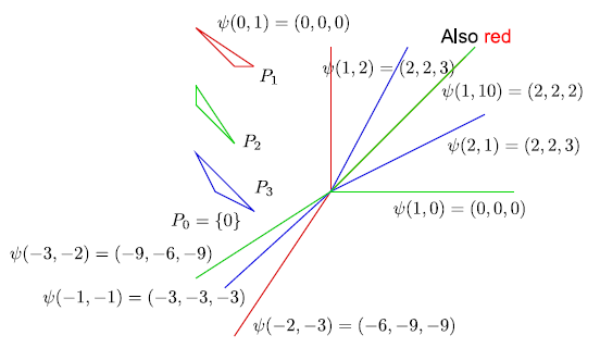
In fact, the Newton polytope of a (reduced) polynomial that defines the closure of the image of is a truncated simplex with vertices . The cones to correspond to the edges of . We explain how to compute a priori the multiplicities (the lengths of the edges) in § 2.6.
Example 2.9 (Non-generic coefficients).
Consider now the rational map associated to the polynomials
The union of the zeros of these ’s (that is, the base locus of ) has a highly singular point at the origin:
![[Uncaptioned image]](2010.02093v1/dibujitosAngie.png)
Let be a (reduced) polynomial that defines the hypersurface parameterized by . Its Newton polytope is the pyramid in with equation cut by the two half-spaces and . Note that it is contained in the convex hull of the support in the generic case in Example 2.8. We depict on the right and on the left:
![[Uncaptioned image]](2010.02093v1/EjGenerico.jpg)
![[Uncaptioned image]](2010.02093v1/EjNOGenerico.jpg)
The tropicalization , instead, is not equal to the union of cones of Theorem 2.5, but bigger. However, we can describe some of the cones in by considering the approach in the proof of Theorem 2.5 and using it as a recipe to find the tropicalization.
In Theorem 2.5, to prove that a cone lies in , the genericity condition is used to ensure that there is a common zero of if and only if and that it satisfies all hypotheses from Lemma 2.7. But this Lemma does not require that the polynomials are generic. Using this idea, we consider for all possible the common zeros of that are not zeros of any polynomial in . If either or , then there is no possible such that have common zeros. If , for all there are points that are not zeros of any . Then, as in the generic case (see Example 2.8),
| (2.16) |
and this set is included in . If the only vector for which there are common zeros of that are not zeros of any for all or of is . For , a possible vector is (although is not the only one). Then, . These 3 are in fact the cones associated to the edges of lying in the coordinate axes.
When looking at , we also need to consider . There is no zero of that is not a zero of . Consider , where and . Then
If and we choose with with , then and Thus, the cone is contained in . The union of this cone with gives the entire cone corresponding to the edge . If , we analyze those such that face has dimension 1. When we obtain the cone which we already have. When there are zeros of that are not zeros of or and we get the cone . Recall that (with the notation of Example 2.8) . Interestingly and as in the generic case, since we already obtained in (2.16) the cone we have that . In the same way, for we obtain that . These cones correspond to the edges and of . The set is a bit more complicated to analyze. If we consider all faces face with dimension 1, both and gives the cone . Via the cones obtained in (2.16), . As we mentioned before, joining with we obtain the cone associated to the edge .
Finer computations are required to find the other five cones associated to the edges of the two new faces of the Newton polytope of , as it is necessary to consider higher order terms in .
2.6. The multiplicities
We complete the description of the tropicalization of the closure of the image of with the computation of the multiplicities of the maximal cones in Theorem 2.5.
Recall that as the variety is irreducible of dimension , is a polyhedral set that can be given the structure of a pure -dimensional fan. Theorem 2.5 gives a description of as a set, and as in [19], this description does not have a natural fan structure. However, every maximal dimensional cone in has a multiplicity . This multiplicity can be computed at any regular point in the cone, by means of [18, Theorem 3.12] and [18, Theorem 5.1].
Consider again the homomorphism of tori in (2.13). Given a regular point in a maximal cone of such that is a finite set of regular points in , equals the sum over all , of the quantities
where the multiplicity of the regular point in is as computed in [18, Theorem 5.1].
Consider the map defined as in (2.9), but for the rational map ). For every with and every coherent collection of faces of adapted to , define index as the index of the lattice in its saturated lattice, when both have rank . Otherwise, index. With this notation, the multiplicity of the regular point in is equal to the sum of
over all sets and all coherent collection of faces of adapted to such that contains . Here, denotes the -dimensional mixed volume.
The following is a simple example of the multiplicity computation via this formula.
Example 2.10.
Let be the polynomials
The rational map has degree 2 and the cones in the tropicalization of its image are and The map has degree 1 and the tropicalization of its image has cones. The following table shows the multiplicity of a regular point in each of them (and the data used to compute it):
.
For example, take a regular point . The set has two points in : the point which is in a cone of multiplicity 2 and the point which lies in a cone of multiplicity 1. Since , the index is 1, but since , the corresponding index is 2. By equation (2.6), .
3. Degree of rational varieties under sparse parametrizations
As before, we consider supports which lie in the nonnegative orthant and generic polynomials with respective supports , such that the rational map from (1.2)
is generically finite and thus rationally parameterizes an irreducible variety of dimension . We give in Theorem 3.3 an explicit formula for its degree in terms of the supports when the coefficients are generic, and which is an upper bound in any case. Our sharp bound for the degree of in Theorem 3.3 for generic coefficients is similar to the bound in Proposition 4 in [12] in case . The upper bound given by the volume of the convex hull of the union of the supports appears in Section 3 in [8]. We give conditions for equalities in the chain (3.5) of inequalities in Theorem 3.9, and we will also show in Example 3.5 that all the inequalities can be strict.
Consider the open set , the incidence variety
| (3.1) |
and the projection
| (3.2) |
Then, coincides with the closure of the image . Moreover, this map is finite iff is finite and both have the same degree. Observe that the polynomials defining don’t have in general generic coefficients with respect to their supports even if have generic coefficients (so the results in [9] do not directly apply). In fact, we compute in Theorem 3.3 studying the following similar genericity question: given a subset of , with cardinality and generic coefficients , when do the polynomials have generic coefficients with respect to their support? If not, which is the number of their common zeros in the torus ?
In order to state our main result in this section, we need to introduce two definitions.
Definition 3.1.
Given a subset and a natural number , denote by the finite subset
| (3.3) |
where and denotes the -th canonical basis vector.
We also define new lattice subsets associated to a collection of finite subsets.
Definition 3.2.
Let with , be a collection of finite lattice subsets. Given with , for any we denote
| (3.4) |
and we define as the mixed volume
We then have
Theorem 3.3.
Consider Laurent polynomials in variables and coefficients in with respective supports , such that the rational map defined as in (1.2) by , is generically finite with . Then,
| (3.5) |
Moreover, the left equality holds when have generic coefficients.
Proof.
As we mentioned, we can assume without loss of generality (possibly after a common translation of the supports) that all exponents are nonnegative. The degree of equals the number of intersection points of with the zero set of generic linear forms in variables with coefficients in , which we will write as follows:
| (3.6) |
Since are generic, we can assume that every intersection point lies in , and it is enough to consider all common zeros of the form for some in the domain of (that is, such that for any ). Such belongs to the variety defined by the following polynomials :
These polynomials have support and so, the number of isolated common zeros in the torus is bounded by by Bernstein’s theorem, with equality in case are generic polynomials with this support. But, depending on the relative positions of , this need not be the case.
A first refinement of this bound is given by the following observation. As the coefficients are generic, for every set with , the system is equivalent by means of row operations to a system of the form
| (3.7) |
where the coefficients are generic. These polynomials have supports for any . By the BKK bound, the system (3.7) has at most isolated common zeros in and by the monotony of the mixed volume, . But still, depending on the original supports , need not have generic coefficients with those supports, even if are generic for their support .
Take and consider the following polynomials in :
| (3.8) |
Denote by the complement in of the union of the zeros of , that is, the domain of definition of . Clearly, there is a bijection between common zeros in of and common zeros in of , so is bounded above by the mixed volume of their supports. But, for generic and generic linear forms , these new polynomials have generic coefficients. Moreover, they do not have common zeros in common in with any . Indeed, no with can vanish if . Take any , for instance . Then, if is a solution in the torus of system (3.8) and , then is also a solution of the system of generic polynomials in variables:
which is a contradiction. So the number of common zeros in is the mixed volume of their supports, , where as in Definition 3.1. Note that replacing by a generic linear combination, we would get the same number of solutions in the torus, and thus, this mixed volume coincides with the mixed volume , as stated in (3.5), and the first inequality follows.
We deduce from the proof of Theorem 3.3 that the generic value of equals . Moreover, we could replace the choice of indices by any subset of of cardinal .
Example 3.4.
Consider the application given by the generic polynomials from Example 2.8. Theorem 3.3 proves the known fact that . Moreover, in this case the first inequality in (3.5)
in the statement is actually an equality. In fact, we can consider the steps in the proof of Theorem 3.3 to verify that We will see below that for general supports the equalities in (3.5) can be strict.
3.1. Sufficient conditions for equality
With the notations from Theorem 3.3, if and are generic, the inequalities in (3.5) are all equalities and equals . But in general, even for generic polynomials, the inequalities may be strict, as we show in the next example.
Example 3.5.
Let , so is a hypersurface in dimension . Consider the generic polynomials in :
Let be their supports sets. We draw their respective convex hulls , .
The closure of the image of the associated rational map is a hypersurface. Let be a reduced polynomial defining . We observe that the degree of the map is , and we can compute , and
In fact, there exists a unique monomial in of maximal degree .
In what follows we will present conditions on the supports for which some of the inequalities in the statement of Theorem 3.3 are actually equalities in case . We will need some preliminary results, which include equivalences due to Bihan and Soprunov (see [2]), and the notion of an essential collection of subsets in Definition 2.3, which was originally introduced in [17]. We then have:
Lemma 3.6.
Let and be finite sets in such that for every . Then, the following statements are equivalent:
- (i)
.
- (ii)
There exists a coherent collection of proper faces of the collection such that the collection is essential, where
- (iii)
There exists a coherent collection of proper faces of the collection such that the collection is either empty or essential.
Proof.
The equivalence between items (i) and (ii) follows from [2, Theorem 3.3]. To see that item (i) is equivalent to item (iii) we apply Bernstein’s Theorem. Let be generic polynomials with support sets . Write . Then if and only if there exists a coherent collection of proper faces of such that the polynomials have a common zero with all non-zero coordinates. But, since are generic, this is equivalent to the set being empty or essential. ∎
Corollary 3.7.
Let be finite sets in . Then, the following are equivalent:
- (i)
.
- (ii)
For every and every face of of codimension , the cardinality of the set is at least .
- (iii)
For every proper face of there exists a nonempty subset such that .
Proof.
Example 3.5, continuation. Recall that by Definition 3.2, for any any with 2 elements and the index in its complement, and both supports are contained in the union . It can be checked that item (iii) in Corollary 3.7 holds and so for all .
The following example shows that the conditions given in items (ii) and (iii) in Lemma 3.6 are different.
Example 3.8.
Consider the finite sets in
Clearly . If we take the coherent collection of faces of associated to the interior normal vector , the collection from item (ii) in Lemma 3.6 is essential. However, the collection from item (iii) is not. On the other hand, if we consider the coherent collection of faces associated to the interior normal vector , the collection from item (iii) Lemma 3.6 is essential but the collection from item (ii) is not.
The following theorem provides a necessary and sufficient condition for the equality for some with . We will denote by the complement of in .
Theorem 3.9.
Let be finite sets in . Fix with . The following statements are equivalent:
- (i)
For every and every face of of codimension and every such that that contains , we have .
- (ii)
.
Proof.
The next theorem provides a sufficient condition for the equality for some with .
Theorem 3.10.
Let be finite sets in . Let be generic polynomials with support and coefficients in such that the rational map from (1.2) is generically finite. Assume with satisfies that for every coherent collection of proper faces of , there exists nonempty subset of such that
Then, deg.
Proof.
Denote and . As in the proof of Theorem 3.3, take generic coefficients so that the system for has common isolated zeros, all of them in the open set .
Example 3.11.
4. Orders of rational hypersurfaces under sparse parametrizations
In this section, we assume that and is a hypersurface in . We will study its order at the origin , which is defined as follows. Let be a (reduced) polynomial such that . Then,
We compute in Theorem 4.2 under an additional condition on the family of supports. As we remarked in the Introduction, depending on the relative positions of the supports it could happen that (that is, the origin is a singular point of the closure of in ) even for generic coefficients, We end with two examples where our proofs can be extended to other cases not falling into the hypotheses of Theorem 4.2.
Before stating Theorem 4.2, we need to introduce a definition.
Definition 4.1.
Let be a family of finite sets in . Given , we call . We say that the family is tame if for any such that and , the family in is not essential (see Definition 2.3).
Note that in case all are equal for all or if all are equal for and consists of a single point (thus are Laurent polynomials with the same support, the case studied in [20]), the family is always tame.
Recall that by Theorem 3.3 the degree of for generic coefficients satisfies , where the notation is given in Definition 3.1.
Theorem 4.2.
Let be a tame family of finite sets in . Let be generic polynomials with respective supports and coefficients in such that the map from (1.2) is generically finite and parameterizes a hypersurface in . Then,
Proof.
Consider generic linear forms with coefficients in , and generic constants for all . As before, consider the open set . We can assume that have common roots, and that they all lie in .
To compute the order at the origin of , we will consider the line in defined by the generic affine linear forms . Notice that this line can be parameterized as
with . The common zeros of the polynomials in are exactly the points
for which . If we consider the polynomial , we have
| (4.1) |
where for all , is a polynomial of degree at most in .
By genericity of and , we can assume that , and . Note that and for all . Hence, if we consider the coefficients of as elementary symmetric functions of the roots , we can easily see that for all . Indeed, assume that for some and consider the non-empty set . Then, the elementary symmetric function has the same negative valuation as , which is a contradiction. Moreover, the minimum power of with a coefficient of valuation is On the other hand, if we now consider as a sum of homogeneous terms of degree to and we evaluate it at , the minimum power of with a coefficient of valuation is . Therefore,
| (4.2) |
We will focus in what follows on bounding the number of points for which . Let be one of them. Since is fixed for all and the supports are tame, let us prove that this implies that if with , then necessarily . Assume first that and recall the notation in (2.5): . Since are generic, they do not all vanish on . Also, if and only if for all However, since the supports are tame, can only have common zeros with all non-zero coordinates when , and so for all As , is a common zero of the polynomials for all . The convex hull of the support of any linear combination of has dimension at most because all supports are contained in the hyperplane with equation . Then, the variety parameterized for all by has dimension at most . The space of lines from a point in through the origin has then codimension at least one in the space of lines in through the origin. Thus, the intersection of with a generic line is empty. Therefore, .
Consider then with . The polynomials
have finitely many common zeros in , being one of those zeros. As in the proof of Theorem 3.3, by taking linear combinations, we can tranform them into polynomials of the form with generic coefficients , and thus its number of common zeros is bounded above by . Moreover, one can take an extra variable and define an associated generic system where
By the genericity of their coefficients, do not have common zeros, and hence common zeros of in correspond to common zeros of the polynomials in . By Bernstein’s Theorem, the number of common roots of equals . Since is smooth, [10, Corollary 6.7.2] ensures that the Jacobian matrix of has nonzero determinant when evaluated at a common zero . This implies that the Jacobian matrix of has valuation zero when evaluated at the common roots of and, by Hensel’s Lemma, each of these common zeros can be lifted to a unique common zero of , for all . We deduce that the number of with is and the result follows from (4.2). ∎
The following proposition presents a sufficient condition for the inequality in the statement Theorem 4.2 to be an equality and the order can be computed in an easier way.
Proposition 4.3.
Under the hypotheses and notation of Theorem 4.2, if there exists such that for all coherent collection of proper faces of , there exists a nonempty subset of such that , then
| (4.3) |
In particular,
| (4.4) |
Proof.
Denote . As the polynomials are generic with respect to their supports, we have by Theorem 3.3 that . Because the supports are tame, we saw in the proof of Theorem 4.2 that and that we can compute as the number of common zeros in of for . Taking linear combinations, this system is equivalent to . Thus, is bounded above by . Now, as in the proof of Theorem 3.10, we introduce a new variable and consider the homotopy:
| (4.5) |
For almost all , its number of common zeros in is . As are generic polynomials, they have common zeros with all non-zero coordinates. Since these zeros are isolated, each is in a germ of curve of zeros of (4.5) not contained in . This implies that . Therefore,
But now, it follows from Lemma 3.6 that , and hence , as claimed. The remaining equality in (4.4) follows from the computation of in the statement of Theorem 4.2. ∎
Example 4.4.
Remark 4.5.
While the hypothesis in the statement of Theorem 4.2 that the supports are tame is sufficient, it is not always necessary. For example, consider the family of lattice sets , , , , . It is easy to check that this family of supports is not tame: for , the set from Definition 4.1 is . However, the family is essential. Even in this case, for generic with those supports, we still have (as in the statement of Theorem 4.2) that
Moreover, the inequality above is an equality. It can be computed that for generic polynomials, , , , and .
Example 4.6.
Consider again Example 2.9 with non-generic coefficients. As in Example 4.4, by applying Bernstein’s Theorem to the polynomial systems in the proof of Theorem 3.3, we can see that all inequalities in Theorem 3.3 are actually equalities and the degree of the surface is . The polytope with vertices has volume . Theorem 4.2 predicts the lower bound for generic systems with those supports, which is also true in this case. To see that, we can follow the steps in its proof, and first verify that there are no with and . Then, we can check that the polynomials for have exactly common zeros in by means of the genericity conditions in Bernstein’s Theorem. Finally, applying [10, Corollary 6.7.2] and Hensel’s Lemma, the order at the origin is exactly .
References
- [1] D. N. Bernstein, The number of roots of a system of equations. Funct. Anal. Appl. 9 (1975), 183–185. translated from Funkts. Anal. Prilozh. 9, No. 3 (1975), 1-4.
- [2] F. Bihan, I. Soprunov, Criteria for Strict Monotonicity of the Mixed Volume of Convex Polytopes, Adv. Geom. 19 (4) (2019), 527–540
- [3] R. Bieri, J. Groves, The geometry of the set of characters induced by valuations. J. Reine Angew. Math. 347 (1984), 168–195.
- [4] M.A. Cueto, Implicitization of Surfaces via Geometric Tropicalization. arXiv:1105.0509
- [5] C. D’Andrea and M. Sombra, The Newton polygon of a rational plane curve, Mathematics in Computer Science 4 (2010), 3–24.
- [6] J. Draisma, A tropical approach to secant dimensions. J. Pure Appl. Algebra 212 (2008), no. 2, 349–363.
- [7] M. Einsiedler, M.M. Kapranov, D. Lind, Non-Archimedean amoebas and tropical varieties. J. Reine Angew. Math. 601 (2006), 139–157.
- [8] I.Z. Emiris, I.S. Kotsireas, Implicit polynomial support optimized for sparseness. Proc. Intern. Conf. Computational science appl.: Part III, Springer, Berlin, 2003, 397–406.
- [9] A. Esterov, A. Khovanskii, Elimination theory and Newton polytopes. Funct. Anal. Other Math. 2 (2008), no. 1, 45–71.
- [10] J.P. Jouanolou, Théorèmes de Bertini et applications. Progress in Math. vol. 42. Basel: Birkhäuser (1983).
- [11] P. Hacking, S. Keel, J. Tevelev, Stable pair, tropical, and log canonical compactifications of moduli spaces of del Pezzo surfaces. Invent. Math. 178 (2009), no. 1, 173–227.
- [12] M.I. Herrero, G. Jeronimo, J. Sabia, On degree bounds for the sparse Nullstellensatz. J. Algebra 534 (2019), 531–544.
- [13] A. Jensen, J. Yu, Computing Tropical Resultants, J. Algebra 387 (2013), 287–319.
- [14] F.V. Kuhlmann, Valuation theoretic and model theoretic aspects of local uniformization. Progress in Mathematics Vol. 181, Birkhäuser Verlag Basel (2000), 381–456.
- [15] T. Markwig, A field of generalized Puiseux series for tropical Geometry. Rend. Semin. Mat. Univ. Politec. Torino 68 (2010), no. 1, 97–92.
- [16] B. Poonen, Maximally complete fields. Enseign. Math., II. Sér. 39, No.1- 2, 87–106 (1993).
- [17] B. Sturmfels, The Newton polytope of the resultant. J. Algebr. Combinatorics, 3:207-236, 1994.
- [18] B. Sturmfels, J. Tevelev, Elimination theory for tropical varieties. Math. Res. Lett. 15 (2008), no. 3, 543–562.
- [19] B. Sturmfels, J. Tevelev, J. Yu, The Newton polytope of the implicit equation. Mosc. Math. J. 7 (2007), no. 2, 327–346, 351.
- [20] B. Sturmfels, J. Yu, Minimal polynomials and sparse resultants. Zero-dimensional schemes (Ravello, 1992), 317–324, de Gruyter, Berlin, 1994.
- [21] B. Sturmfels, J. Yu, Tropical implicitization and mixed fiber polytopes. Software for algebraic geometry, 111–131, IMA Vol. Math. Appl., 148, Springer, New York, 2008.