IEEEexample:BSTcontrol
NATSA: A Near-Data Processing Accelerator
for Time Series Analysis
Abstract
Time series analysis is a key technique for extracting and predicting events in domains as diverse as epidemiology, genomics, neuroscience, environmental sciences, economics, and more. Matrix profile, the state-of-the-art algorithm to perform time series analysis, computes the most similar subsequence for a given query subsequence within a sliced time series. Matrix profile has low arithmetic intensity, but it typically operates on large amounts of time series data. In current computing systems, this data needs to be moved between the off-chip memory units and the on-chip computation units for performing matrix profile. This causes a major performance bottleneck as data movement is extremely costly in terms of both execution time and energy.
In this work, we present NATSA, the first Near-Data Processing accelerator for time series analysis. The key idea is to exploit modern 3D-stacked High Bandwidth Memory (HBM) to enable efficient and fast specialized matrix profile computation near memory, where time series data resides. NATSA provides three key benefits: 1) quickly computing the matrix profile for a wide range of applications by building specialized energy-efficient floating-point arithmetic processing units close to HBM, 2) improving the energy efficiency and execution time by reducing the need for data movement over slow and energy-hungry buses between the computation units and the memory units, and 3) analyzing time series data at scale by exploiting low-latency, high-bandwidth, and energy-efficient memory access provided by HBM. Our experimental evaluation shows that NATSA improves performance by up to 14.2 (9.9 on average) and reduces energy by up to 27.2 (19.4 on average), over the state-of-the-art multi-core implementation. NATSA also improves performance by 6.3 and reduces energy by 10.2 over a general-purpose NDP platform with 64 in-order cores.
1 Introduction
A time series is a chronologically ordered set of samples of a real-valued variable that can contain millions of observations. Time series analysis is used to analyze information in a wide variety of domains [92]: epidemiology, genomics, neuroscience, medicine, environmental sciences, economics, and more. Time series analysis includes finding similarities (motifs [25]) and anomalies (discords [48]) between every two subsequences (i.e., slices of consecutive data points) of the time series [109, 101]. There are two major approaches for motif and discord discovery: approximate and exact algorithms [65]. Approximate algorithms [25] are faster than exact algorithms, but they can provide inaccurate results or limited discord detection, which cannot be tolerated by many applications (e.g., vehicle safety systems [85]). Unlike approximate algorithms, exact algorithms [67] do not yield false positives or discordant dismissals, but can be very time-consuming on large time series data. Thus, anytime versions (aka interruptible algorithms) of exact algorithms are proposed to provide approximate solutions quickly [108, 112] and can return a valid result even if the user stops their execution early.
The state-of-the-art exact anytime method for motif and discord discovery is matrix profile [108], which is based on Euclidean distances and floating-point arithmetic. Fig. 1 depicts a naive example of anomaly detection using matrix profile, where the sinusoidal signal has an anomaly between values 250 and 270. The matrix profile output of this time series shows low values for the periodic subsequences of it as they are very similar to the other subsequences, and higher values for the anomalies and their neighboring subsequences.
We evaluate a recent CPU implementation of the matrix profile algorithm [112] on a real multi-core machine (Intel Xeon Phi KNL [95]) and observe that its performance is heavily bottlenecked by data movement. In other words, the amount of computation per data access is not enough to hide the memory latency and thus time series analysis is memory-bound. This overhead caused by data movement limits the potential benefits of acceleration efforts that do not alleviate data the movement bottleneck in current time series applications.
Several CPU and GPU implementations of matrix profile have been proposed in the literature [108, 44, 112, 113]. However, these acceleration efforts still require transferring the time series data from the main memory to the CPU/GPU cores, leading to the data movement bottleneck. Near-Data Processing (NDP) [68, 34, 33, 43, 103, 5, 12, 24, 41, 49, 62, 90, 7, 89, 30, 26, 6, 31, 57, 16, 17, 18, 42, 52, 19, 40, 86, 60, 94, 78, 88, 93, 40, 87, 79, 23, 50, 51, 50, 51] is a promising approach to alleviate data movement by placing processing units close to memory. As a result, NDP solutions have the potential to improve system performance and energy efficiency when they are carefully designed with low-cost and low-overhead near data processing cores for memory-bound applications [30, 16, 6, 7, 68, 33, 34, 43, 31, 57, 52, 17, 38, 72, 70].
Our goal in this work is to enable high-performance and energy-efficient time series analysis for a wide range of applications, by minimizing the overheads of data movement. This can enable efficient time series analysis on large-scale systems as well as embedded and mobile devices, where power consumption is a critical constraint (e.g., heart beat analysis on a mobile medical device to predict a heart attack [58]). To this end, we propose NATSA, the first Near-Data Processing Accelerator for Time Series Analysis. The key idea of NATSA is to exploit modern 3D-stacked High Bandwidth Memory (HBM) [55, 56] along with specialized custom processing units in the logic layer of HBM, to enable energy-efficient and fast matrix profile computation near memory, where time series data resides. NATSA supports a wide range of time series applications thanks to matrix profile’s generality and flexibility.
Our evaluation shows that NATSA provides up to 14.2 (9.9 on average) higher performance and up to 27.2 (19.4 on average) lower energy consumption compared to a state-of-the-art multi-core system. NATSA consumes 11.0 and 4.1 less energy over optimized implementations of matrix profile on an Intel Xeon Phi KNL [27] and NVIDIA GTX 1050 GPU [44], respectively. NATSA has 9.6 and 1.8 smaller area than these two accelerators, at equivalent performance points. NATSA outperforms a general-purpose NDP platform by 6.3 while consuming 10.2 less energy.
This work makes the following contributions:
- •
We propose NATSA, the first near-data processing accelerator for accelerating time series analysis using modern 3D-stacked High Bandwidth Memory (HBM).
- •
We propose a new workload partitioning scheme that preserves the anytime property of the algorithm, while providing load balancing among near-data processing units.
- •
We perform a detailed analysis of NATSA in terms of both performance and energy consumption. We compare different versions of NATSA (DDR4 [46] and HBM [55]) with four different architectures (8-core CPU, 64-core CPU, GPUs and NDP-CPU) and find that NATSA provides the highest performance and lowest energy consumption.
2 Background
2.1 Time Series Analysis: The matrix profile
A time series is a sequence of data points , where , collected over time. A subsequence of , also called a window, is denoted by , where is the index of the first data point, and is the number of samples in the subsequence, with , and .
The state-of-the-art exact anytime method for time series analysis is matrix profile [108]. When analyzing a time series, the profile is maintained as another time series that represents the most similar neighbor for a particular subsequence of the original time series. The similarity between two subsequences and can be calculated using the z-normalized Euclidean distance, which is defined as follows.
| (1) |
where is the dot product of and ; and are the mean and the standard deviation of the points in , respectively. These statistics are computed in time [81].
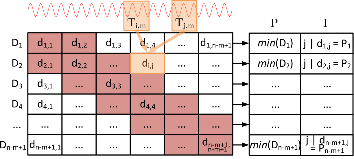
Using the distance in Eq. 1, the matrix profile algorithm solves the similarity search problem in three steps. First, it builds a symmetric matrix , called distance matrix. Each cell in , , stores the distance between two subsequences, and . Second, it creates an array of size , called profile. Each cell in keeps the minimum distance recorded in the row of . Third, it allocates an array that is of the same size as , called profile index, such that if . This way, contains the minimum distances between subsequences, while is the vector of “pointers” to the location of these subsequences within the time series.
Fig. 2 depicts an example of the distance matrix , the profile , and the profile index . The neighboring subsequences of are highly similar to it (i.e., ) due to overlapping between them. The algorithm excludes these subsequences from the computation to avoid false positives, by defining an exclusion zone for each subsequence. It follows the approach in [112], where the exclusion zone of is (i.e., ends at of the time series).
2.2 The SCRIMP Implementation
The state-of-the-art CPU-based implementation of the matrix profile algorithm is SCRIMP [112]. We use an optimized version of SCRIMP [27] as baseline for our work, since it has the best convergence properties and takes advantage of multithreading and vectorization. The key mechanism behind optimized SCRIMP is that the dot product in Eq. 1 can be calculated incrementally in the diagonals of as follows:
| (2) |
According to Eq. 2, except for the first dot product, the remaining cells of a diagonal can be calculated using the values from the immediate upper left cells. This fact significantly reduces the number of multiplications and additions needed.
Algorithm 1, optimized SCRIMP [27], exploits both thread-level parallelism and vectorization. First, it precalculates the means and standard deviations of every subsequence of the time series (line 1), and initializes the profile vector (lines 3-4). Second, it computes the diagonals (see Fig. 2) using the loop in line 5. The variable nDiag is the number of diagonals of assigned to each thread. These diagonals can be ordered in the diag vector (line 6) a) randomly, enabling the anytime property of the algorithm, or b) sequentially, discarding the anytime property but allowing for optimizations [112] (e.g., exploiting data locality of consecutive diagonals).
Note that only and are allocated in memory, since storing can lead to large memory consumption for large series due to the memory footprint (i.e., the values of are calculated on the fly, updating and when needed). For each diagonal, the algorithm first computes the dot product of the first pair of subsequences in line 7 using the dotProduct function, which is vectorized. Second, it calculates the distance according to Eq. 1 (line 8). Third, it checks and replaces the corresponding profile element with the new distance provided that the calculated one is smaller (lines 9-10).
The algorithm addresses the imposed data dependency due to the dot product update between the elements in the diagonal with the following steps: 1) it pre-computes the add terms in Eq. 2 in batches of size in a vectorized manner (lines 13-14); 2) it adds the previous dot product to the first new one (line 15); 3) it sequentially updates the remaining dot products in the batch (lines 16-17) saving the last one for the next iteration of the diagonal (line 18); 4) it computes the distance as well as the profile update in a vectorized way (lines 19-22). As a result, all loops are fully vectorized except the one in lines 16-17.
2.3 NDP and 3D-Stacked Memory
Near-Data Processing (NDP) [68, 34, 33, 43, 103, 5, 12, 24, 41, 49, 62, 90, 7, 89, 30, 26, 6, 31, 57, 16, 17, 18, 42, 52, 19, 40, 86, 60, 94, 78, 88, 93, 40, 87, 79, 23, 50, 51] is a promising paradigm to reduce the data movement between CPUs and memory by placing simple general-purpose processors [42, 6, 16] or application-specific accelerators [43, 111, 52, 19, 16, 7] in or close to the logic layer of 3D-stacked memory. Generally, NDP can provide performance benefits for memory-bound applications when they exhibit one or more of the following major properties: 1) requiring higher memory bandwidth than available in the system, 2) being sensitive to memory access latency [70], or 3) performing irregular memory accesses, such that they cannot effectively benefit from cache hierarchy of conventional CPU architectures. .
Recent advances in die-stacking technologies have enabled the integration of multiple layers of DRAM arrays in a single package. A 3D-stacked memory consists of several memory dies, one on top of each other, connected using Through-Silicon Vias (TSV) [55, 56]. NDP locates low-power processing units inside the logic layer of 3D-stacked memory, to harness the significantly higher bandwidth and the lower latency provided while consuming less energy. The most prominent 3D-stacked memory technologies are High Bandwidth Memory (HBM) [47] and Hybrid Memory Cube (HMC) [39], but there are several others [53, 35].
3 Motivation
NATSA is motivated by two key observations: First, time series motif and discord discovery are two of the most important analysis primitives for a wide variety of applications. Besides the applications mentioned in Section 1, we can find these primitives applied to bioinformatics [14, 10, 8], speech processing [32], robotics [80], weather prediction [64], entomology [97], geophysics [21], finance [20], communication engineering [54], and electroencephalography [45].
Second, memory is the main bottleneck in time series analysis. We characterize the performance of a state-of-the-art CPU-based multithreaded and vectorized implementation of SCRIMP, developed in [27]. We run SCRIMP [27] on an Intel Xeon Phi 7210 processor, with 64 cores and 256 hardware threads, using two types of memory (DDR4 and HBM) available in this architecture. In Fig. 3, we present the performance results normalized to 1 thread (lines) and utilized memory bandwidth (bars) of SCRIMP. We observe that, when using DDR4, the performance of SCRIMP does not scale beyond 32 threads, whereas the higher memory bandwidth provided by HBM enables SCRIMP to scale up to 128 threads. This shows that SCRIMP’s performance saturates on many-core architectures, because the achievable bandwidth saturates when the number of threads increases. To know the cause for this memory boundedness we perform the next experiment.
We perform the roofline analysis as we show in Fig. 4. We observe that the arithmetic intensity of SCRIMP is significantly low. The confirms that the memory boundedness of SCRIMP is due to the low arithmetic intensity of the algorithm, which leads processing cores to be underutilized. Based on all these observations, we conclude that the performance of the state-of-the-art CPU-based implementation of the matrix profile, SCRIMP [27], is heavily bottlenecked by available memory bandwidth and data movement. Our goal is to reduce the data movement bottleneck of SCRIMP by building an NDP accelerator that matches the compute throughput of processing elements with the available memory bandwidth.
4 NATSA Architecture
Our Near-Data Processing Accelerator for Time Series Analysis, NATSA, is designed to 1) fully exploit the memory access parallelism and high memory bandwidth offered by HBM, and 2) employ the required amount of computing resources to provide a balanced solution. NATSA is built next to the HBM memory and exploits the full HBM bandwidth available. NATSA consists of multiple processing units (PUs) that efficiently compute the diagonals of matrix profile in a parallel fashion. The PUs are designed to compute diagonals using a vectorized approach to process a batch of elements of a diagonal at the same time. Each PU includes energy-efficient floating-point units [29], bitwise operators, and registers (See Table 3 in Sect. 6.3). Each PU communicates with the HBM memory via a controller connected to one of the 8 memory channels provided by HBM.
4.1 NATSA Processing Units (PUs)
Each NATSA PU consists of four hardware components: the Dot Product Unit (DPU), the Distance Compute Unit (DCU), the Profile Update Unit (PUU), and the Dot Product Update Unit (DPUU), as we show in Fig. 5. We share the floating-point arithmetic operators (e.g., multipliers) among those hardware components to minimize idle cycles and enable reusability. The control unit ( in Fig. 5) is a state machine that orchestrates the execution flow of a PU. The multiplexers ( in Fig. 5) choose between the output of DPU and DPUU based on a signal from the control unit, so that the DCU can take advantage of Eq. 2, starting from the second element of the diagonal all the way down to the last. We replicate those hardware components to compute different elements of a diagonal in parallel, using the vectorized approach outlined in Section 2.2. The diagonal assignment is pre-calculated in the host CPU, which sends the indices of the to-be-computed diagonals to each NATSA PU. Finally, each NATSA PU uses its own 1KB scratchpad memory to temporarily store fixed-size auxiliary data, such as the window size or configuration parameters.
The execution flow through the hardware components of a PU includes the following six steps:
- 1.
Dot product computation of the first element of the diagonal. The DPU calculates the dot product between the first pair of subsequences of the diagonal ( and ) by using the time series input, and the window size, m, which is used to signal the end of each subsequence. This hardware component vectorizes the operation and outputs the result, , for the next step.
- 2.
Euclidean distance computation of the first element of the diagonal. The DCU computes the first Euclidean distance of each diagonal following Eq. 1, using the dot product computed by the DPU . The values of and are precomputed by the host CPU in negligible time ( [81]) with respect to the total execution time. This simplifies the design of the PU.
- 3.
First profile update. If the Euclidean distance calculated in the DCU, , is lower than that stored in the profile for both subsequences, the PUU updates the profile vector and profile index vector, and .
- 4.
Dot product update. The dot product of the second and successive cells in the diagonal is calculated from the previous cell. It is computed in the DPUU by subtracting the first product and adding the new one to , as shown in Eq. 2. This hardware component is replicated to enable vectorization and is pipelined with the DCU and the PUU.
- 5.
Second and successive Euclidean distance computations. The DCU computes again the Euclidean distance, but now it obtains from the DPUU. The DPUU hardware component is replicated for vectorization of the dot product update calculations.
- 6.
Second and successive profile updates. The PUU updates the profile vector and profile index vector, if needed. This hardware component is replicated to perform several updates at a time.
4.2 Workload Partitioning Scheme
Computing the diagonals of the distance matrix may lead to load imbalance among the PUs, because those diagonals have different lengths. To avoid this imbalance, we propose a static partition scheduling scheme which depends only on the size of the time series and the exclusion zone.
The way we tackle this problem is by assigning a set of pairs of diagonals to each NATSA PU such that the sum of their elements is equal to the number of cells of the main diagonal of the distance matrix minus the number of cells of the exclusion zone, .
Fig. 6 illustrates an example with two PUs, PU0 and PU1, a distance matrix for a time series of cells, a window size of , and an exclusion zone of 1 diagonal (crossed out rectangles). In this case, the number of elements that each pair of diagonals assigned to a PU should have is . Comparing a subsequence with itself gives zero distance value. As a consequence, the algorithm treats the main diagonal as exclusion zone and avoids computing it. The first diagonal of non-zero values, which starts in column and is represented with crossed out rectangles, belongs to the exclusion zone (see Fig. 2), so NATSA PUs also skip it.
Discarding the computation of the main diagonal and the diagonals in the exclusion zone, both PUs have to compute the diagonals from columns to . To perform this efficiently and maintain the anytime property of SCRIMP, in the first step, PU0 is assigned the first and last diagonal (9 elements in total), and PU1 is assigned the second and the penultimate diagonal (totalling 9 elements as well). In the second step, PU0 computes the third and the third-to-last diagonal, whereas PU1 computes the fourth and fifth diagonals.
Our proposed scheduling scheme can be used in two ways: 1) Randomly ordering the indices of diagonals that each PU has to compute. Using this approach, we are able to preserve the anytime property of the algorithm, since if the execution is interrupted, the user obtains a partial exploration of the whole time series (i.e., events from any point of the time series can be detected). 2) Sequentially ordering the indices of diagonals that each PU has to compute. This approach violates the anytime property (i.e., only events up to the interruption point can be detected), but allows for further optimizations (e.g., exploiting data locality between consecutive diagonals).
Data mapping. Each PU has access to its corresponding portion of the time series and statistic vectors, and works with replicated profile and profile index vectors. This approach simplifies the overall architecture, enabling the use of many PUs without having to synchronize between them. NATSA assigns multiple diagonals to each PU with the specific scheduling scheme described in this section.
4.3 Programming Interface
In this section, we introduce the API to invoke NATSA from a host processor. While conventional loosely-coupled accelerators (e.g., GPUs or FPGAs) have their own memory, where data must be transferred to from the host’s memory, NATSA is a tightly-integrated NDP accelerator, located between the host CPU and main memory. Thus, there is no need to transfer any data between the host memory and the accelerator memory, as loosely-coupled accelerators require. The user is responsible for 1) allocating the time series () and 2) providing the window length (). NATSA will provide the user the profile vector () and profile index vector () in return. The size of the exclusion zone ( by default) can be also passed as a parameter ().
Algorithm 2 outlines the NATSA API. First, NATSA function precalculates the statistics () (line 2) in the host CPU and allocates the private vectors () to NATSA’s PUs (line 3).
Second, NATSA function implements the diagonal scheduling scheme presented in the previous section, setting the diagonals to be computed by each PU in (line 4). Third, it initiates the accelerator (line 5), which starts the computation, and the host CPU waits for all the processing units to finish. Once the computation finishes, the host CPU performs the final reduction of the private vectors (line 6) and the user can find the results in the and vectors. The conf argument (line 1), besides holding configuration parameters for the accelerator, allows for future extensions, such as using other distance metrics (e.g., Pearson correlation [113]).
5 Methodology
We describe the simulation environment and the workload we use to evaluate the performance of NATSA.
5.1 Simulation Environment
We simulate general-purpose cores using an in-house integration of ZSim [84], whose front-end is Pin [63], with Ramulator [53] [82]. ZSim is a simulator which can model 1) general purpose cores (both in-order and out-of-order cores), and 2) the conventional cache hierarchy. Ramulator is a cycle-level and extensible DRAM simulator that provides a wide variety of memory models, including DDR4 [46] and HBM [55]. We use McPAT [59] for power estimations.
For the NATSA accelerator, we use the gem5 [15] and Aladdin [91] integration developed in [96]. Aladdin provides performance, area, and power estimations for a system-on-chip accelerator by requiring the equivalent C implementation of the accelerator design. Aladdin estimates the performance, power, and area of the accelerator within 0.9%, 4.9%, and 6.6% compared to that provided by RTL flows, but over faster [91]. As Aladdin does not model the memory subsystem, we need to simulate it using gem5.
For a fair comparison, we evaluate our baseline platform (see the evaluated platforms below) in both ZSim and gem5 frameworks using the same workload (see Section 5.2). We obtain up to 10% simulated time reduction using ZSim with respect to gem5 (i.e., the baseline system performs slightly better with ZSim). As a consequence, the performance benefits of NATSA with respect to the baseline simulated using gem5, would be even higher. However, we choose ZSim since simulations of manycore systems with ZSim are orders of magnitude faster than gem5 simulations [84], and this allows for the evaluation of general-purpose core platforms with large time series. For both general-purpose cores and accelerators, we obtain the power consumption of the memory system using the Micron Power Calculator [2], which we feed with the bandwidth usage from Ramulator and gem5, respectively.
Using these simulation environments, we define several representative hardware platforms for the evaluation:
- •
DDR4-OoO (Baseline): A conventional DDR4-based system with eight four-wide out-of-order cores at 3.75GHz. Each core has 32KB private L1 instruction/data caches and a private 256KB L2 cache. The cores share an 8MB L3 cache. The main memory is a dual channel 16GB DDR4-2400 with 38.4GB/s of memory bandwidth.
- •
DDR4-inOrder: A conventional architecture using 64 in-order cores at 2.5GHz. Each core has only a single level of private 32KB instruction/data caches. The main memory is the same DDR4 as in the baseline system. We use this simple core-cache configuration to compare with the following NDP general-purpose-core system.
- •
HBM-OoO: An NDP architecture with eight four-wide out-of-order cores at 3.75GHz. Each core has 32KB private L1 instruction/data caches and a private 256KB L2 cache. The main memory is a 4GB 3D-stacked HBM2 that provides a throughput of 256GB/s.
- •
HBM-inOrder: An NDP architecture with 64 in-order cores at 2.5GHz. Each core has a single level of private 32KB instruction/data caches. The main memory is a 4GB 3D-stacked HBM2 that provides a throughput of 256GB/s.
- •
NATSA: Our NDP accelerator with 48 PUs at 1GHz. Each PU has access to a private scratchpad memory of 1KB. The main memory is the same 4GB 3D-stacked HBM2 as in the HBM-OoO and HBM-inOrder platforms.
5.2 Workload
We use two real datasets and five synthetic datasets to evaluate the performance of NATSA against state-of-the-art architectures. The two real datasets are electrocardiogram (ECG) and seismology data obtained from [98] and [107]. We use these real datasets to 1) verify the correctness of the matrix profile computed by NATSA (the same approach used in [107]) and 2) evaluate the effect of using single-precision versus double-precision (see Section 6.5). We generate the five synthetic datasets of different representative lengths [112] for performance evaluation using MATLAB, as shown in Table 1.
| Time Series | rand_128K | rand_256K | rand_512K | rand_1M | rand_2M |
|---|---|---|---|---|---|
| Length (n) | 131072 | 262144 | 524288 | 1048576 | 2097152 |
6 Evaluation
In this section, we first evaluate NATSA’s performance, comparing it to the general-purpose platforms (DDR4-OoO, DDR4-inOrder, HBM-OoO, and HBM-inOrder). Second, we compare NATSA to both simulated and real architectures (e.g., many-core CPUs and GPUs [44]) in terms of power consumption and area. Third, we present a design space exploration of NATSA. Fourth, we analyze the performance of general-purpose cores and their bottlenecks. Finally, we evaluate SCRIMP in terms of precision and sensitivity to subsequence lengths ().
6.1 Performance of NATSA
We evaluate the performance of two NATSA designs using single-precision (SP) and double-precision (DP), respectively. We present normalized performance of NATSA-DP with respect to the baseline platform (DDR4-OoO) in Fig. 7, using double-precision data. NATSA achieves significant performance improvements, up to 14.2 (9.9 on average) over the baseline system for large time series, and 6.3 over HBM-inOrder for all sizes. We observe that NATSA’s speedup increases as the time series length becomes larger. This is because the arithmetic intensity decreases when the ratio of time series length () to window size () increases. Dot product update (Section 2.2) causes the first dot product to take a significant part of the computation for shorter diagonals (lower to ratio). The cache hierarchy of the baseline system accelerates the first dot product. Conversely, a greater to ratio results in longer diagonals with the first dot product being less significant with respect to the total execution time, reducing the observed benefits of a cache hierarchy.
We evaluate the performance of the single-precision NATSA design.11 1 We note that NATSA experiments are carried out with the gem5-Aladdin simulation framework, and the other platforms are evaluated with the ZSim-Ramulator framework (baseline system included). As mentioned in Section 5.1, simulated times are slightly shorter for ZSim, so the actual gains of NATSA would likely be even greater what we report. Table 2 presents the average execution time for the analyzed datasets. NATSA-SP, which provides higher performance with similar area cost to NATSA-DP, outperforms NATSA-DP by up to 1.75, DDR4-OoO-DP by up to 24.9 and HBM-inOrder-DP by up to 11.1 for large time series.
| rand_128K | rand_256K | rand_512K | rand_1M | rand_2M | |
|---|---|---|---|---|---|
| DDR4-OoO-DP | 14.72 | 77.55 | 414.55 | 2089.05 | 9810.30 |
| DDR4-OoO-SP | 6.46 | 44.47 | 207.85 | 1106.36 | 5206.75 |
| HBM-inOrder-DP | 14.95 | 64.20 | 262.33 | 1071.03 | 4347.38 |
| HBM-inOrder-SP | 8.16 | 35.68 | 130.23 | 625.27 | 2466.69 |
| NATSA-DP | 2.47 | 10.37 | 42.45 | 171.72 | 690.65 |
| NATSA-SP | 1.41 | 5.91 | 24.19 | 97.84 | 393.45 |
We conclude that NATSA provides the highest performance compared to modern general-purpose platforms.
6.2 Power, Energy and Area Consumption
Power and Energy Consumption. We compare the power and energy consumption of NATSA versus other existing hardware platforms in Figures 8 and 9. We use McPAT and Micron Power Calculators to evaluate energy consumption for the general-purpose platforms, getting the number of stalls and bandwidth usage from ZSim-Ramulator. For NATSA, we add Aladdin’s energy estimations to the values obtained from the Micron Power Calculator. We also obtain energy measurements from real executions on GPUs using NVVP [4] and on CPUs using PCM [1], to compare NATSA with real platforms.
Fig. 8 shows the dynamic power consumption of each simulated or real hardware platform. We observe that NATSA has the lowest power consumption, and most of its power is consumed by memory.
Fig. 9 shows the energy consumption of each simulated or real platform, for the computation of a time series of 524,288 elements (rand_512K) using double-precision. To calculate the energy consumption, we compute the power-delay product with the measured instantaneous power consumption and the execution time. NATSA reduces energy consumption by 27.2 (19.4 on average) over the baseline platform (DDR4-OoO), and by 10.2 over an NDP architecture with general-purpose cores (HBM-inOrder). NATSA consumes 1.7, 4.1, and 11.0 less energy than an NVIDIA Tesla K40c GPU [76], NVIDIA GTX 1050 GPU [3], and Intel Xeon Phi KNL [95], respectively. We conclude that NATSA is the most energy-efficient evaluated platform for matrix profile.
Area. We provide a scaled area comparison in Fig. 10. We observe that NATSA requires 9.6, 7.9, 3, and 1.8 less area than an Intel Xeon Phi KNL (14nm), NVIDIA Tesla K40c (28nm), Intel Core i7 (32nm), and NVIDIA GTX 1050 (14nm).
We conclude that NATSA (at 45nm technology node) is the platform that requires the least area, while using the largest technology node (i.e., 45nm) compared to other evaluated architectures. Using a more recent and smaller technology node (e.g., 15nm instead of 45nm) could additionally reduce NATSA’s energy consumption by 4 and area by 3 [83].
6.3 NATSA Design Space Exploration
We explore the key design choices of NATSA so that we deploy the exact number of PUs that saturate the memory bandwidth available, while minimizing the area and power consumption of the accelerator. We evaluate the use of HBM memory,22 2 We also explore the use of DDR4 memory, where 8 PUs are enough to saturate the available memory bandwidth and the performance obtained is similar to the DDR4-inOrder platform (4% difference). where we find that 48 PUs make the accelerator balanced between memory bandwidth and compute parallelism, as 64 PUs result in a memory-bound accelerator, whereas 32 PUs a compute-bound one. Table 3 details the design parameters of NATSA for HBM. NATSA has 48 PUs which run at a frequency of 1GHz, fabricated at 45nm process. Implementations of NATSA with lower technology nodes would provide smaller area footprint and improved energy efficiency. Table 3 shows the components in a PU depending on the data precision: 1) double-precision (DP), and 2) single-precision (SP).
| Parameter/Component | PU-DP | NATSA-DP | PU-SP | NATSA-SP |
|---|---|---|---|---|
| Mem. bandwidth (GB/s) | 5 | 240 | 5 | 240 |
| Peak power (W) | 0.1 | 4.8 | 0.08 | 3.84 |
| Area () | 1.62 | 77.76 | 1.51 | 72.48 |
| FP Multipliers/Adders | 16/14 | 768/672 | 64/36 | 3072/1728 |
| Integer Adders | 16 | 768 | 64 | 3072 |
| Bitwise Operators | 2 | 96 | 2 | 96 |
| Registers | 108 | 5184 | 267 | 12816 |
6.4 Performance of General-Purpose Cores
We evaluate the speedup over the baseline (DDR4-OoO) and memory bandwidth usage of SCRIMP, calculated using the ZSim-Ramulator framework for the DDR4-OoO, DDR4-inOrder, HBM-OoO and HBM-inOrder platforms using double-precision time series of different lengths (), in Fig. 11.
We report execution time of the baseline (DDR4-OoO) on top of the respective performance bars in Fig. 11. Based on these results, we make three key observations. First, the DDR4-OoO platform does not use the peak available bandwidth of DDR4 (i.e., 38.4GB/s). We reinforce this observation with our HBM-OoO evaluation which replaces DDR4 with higher bandwidth HBM. HBM-OoO platform improves performance by only 7%, which means that providing more bandwidth does not significantly affect performance. This is because both platforms are compute-bound when executing SCRIMP. Second, the 64 lightweight cores of DDR4-inOrder slightly outperform the 8 complex cores of DDR4-OoO when elements (i.e., rand_1M dataset). This is because shorter time series can fit in the L3 cache. For long time series, the higher parallelism provided by the in-order platform enables higher memory-level parallelism [72, 69, 36, 71, 70, 73] and higher memory bandwidth demand, where DDR4 bandwidth becomes a bottleneck, resulting in a memory-bound system. Third, the HBM-inOrder platform provides up to 2.25 speedup over the baseline (DDR4-OoO), and consumes only 17% of the HBM’s peak bandwidth with the largest dataset evaluated. In this case, even though performance is improved, the application is still compute-bound and simple NDP general-purpose cores cannot fully exploit the bandwidth provided by HBM (256GB/s)33 3 Based on the memory bandwidth usage and McPAT, we estimate that a general-purpose based architecture would need 128 OoO cores (area 688mm2, TDP 1137W, 18nm) or 384 in-order cores (area 164mm2, TDP 126W, 18nm) to take full advantage of the maximum bandwidth provided by HBM. for the largest dataset we evaluate, which means that large datasets can be comfortably accommodated.
We conclude that general-purpose platforms provide less performance than NATSA’s balanced design because they do not effectively exploit the memory bandwidth of HBM.
6.5 Accuracy and Sensitivity to Window Size
Accuracy. We explore how the accuracy of the SCRIMP implementation is affected by changing the precision of the data representation. We use real data obtained from [98] and [107], as discussed in Section 5.2. Fig. 12 presents the output obtained for an electrocardiogram (ECG) and for seismology data using two precision values. We observe that events are still detectable even when reducing the precision from double to single precision. This observation can be exploited to improve performance and reduce energy consumption, by operating on smaller arithmetic units and less memory footprint.
Sensitivity to the subsequence length. We also perform a sensitivity analysis to the subsequence length (). We observe that, when the proportion between and is less than two orders of magnitude, the performance of SCRIMP in all platforms is significantly affected by . For example, when increasing from 1,024 to 16,384 in a time series of 131,072 elements, the execution time of SCRIMP reduces by 41%. However, when the time series length is large enough compared to the subsequence length, performance of SCRIMP is affected by a smaller amount. For instance, when increasing from 1,024 to 16,384 in a time series of 2,097,152 elements, the execution time of SCRIMP reduces by 13%. This is because the computation of the first element of each diagonal involves the dot product calculation without any reutilization.
7 Related Work
To our knowledge, this is the first work that proposes a near-data processing accelerator for time series analysis. In this section, we briefly discuss prior work related to time series motif discovery and application-specific NDP accelerators.
Multiple techniques exist for time series motif and discord discovery [77, 25, 99, 28, 106, 100, 67, 22, 74, 75, 61, 66, 110, 37, 102, 13]. A survey on time series motif discovery algorithms can be found in [101]. These implementations are approximate or exact [65] in finding motifs and discords, which affects the time complexity of the algorithm. Exact motif and discord discovery processing of exceptionally large time series can be very time-consuming [113]. Consequently, anytime algorithms [108] are proposed to return a valid solution even if they are interrupted, and are expected to find better solutions the longer they run. Matrix profile [108] is the state-of-the-art exact anytime algorithm for time series motif and discord discovery. There are several implementations of matrix profile, including STAMP [108], STOMP [44], SCRIMP [112] and SCAMP [113]. SCRIMP is the state-of-the-art CPU-based implementation. Prior acceleration approaches to time series analysis [44, 112] mainly focus on accelerating STOMP and PreSCRIMP [112] on GPUs. Recently, SCAMP [113] framework combines a host (either a local machine or a server in a compute cluster) and workers that follow the directions from the host (either other CPUs in the cluster or accelerators such as GPUs). A SCRIMP version tuned for a many-core CPU (Intel Xeon Phi KNL) using vectorization can be found in [27].
Recent works explore Near Data Processing [68, 34, 33, 43, 103, 5, 12, 24, 41, 49, 62, 90, 7, 89, 30, 26, 6, 31, 57, 16, 17, 18, 42, 52, 19, 40, 86, 60, 94, 78, 88, 93, 40, 87, 79, 23] for various applications using accelerators or general-purpose cores. In [26], ARM cores are used as NDP compute units to improve data analytics operators (e.g., group, join, sort). IMPICA [43] is an NDP pointer chasing accelerator. Tesseract [6] is a scalable NDP accelerator for parallel graph processing. TETRIS [31] is an NDP neural network accelerator. Lee et al. [57] propose an NDP accelerator for similarity search. GRIM-Filter [52] is an NDP accelerator for pre-alignment filtering [105, 9, 104, 11, 10] in genome analysis [8]. Boroumand et al. [16] analyze the energy and performance impact of data movement for several widely-used Google consumer workloads, providing NDP accelerators for them. CoNDA [17] provides efficient cache coherence support for NDP accelerators. Finally, an NDP architecture [38] has been proposed for MapReduce-style applications.
8 Conclusion
We introduce NATSA, the first Near-Data-Processing (NDP) accelerator for time series analysis. NATSA 1) exploits the memory bandwidth of high-bandwidth memory (HBM) to analyze time series data at scale for a wide range of applications, 2) improves energy efficiency and execution time by using specialized low-power arithmetic units close to HBM memory, and 3) provides a novel workload scheduling scheme to prevent load imbalance and preserve the anytime property. NATSA outperforms the hardware platforms we evaluate in terms of performance, energy consumption and area requirements. We conclude that NATSA is an efficient NDP accelerator for time series, and hope that this work inspires future research directions in NDP for time series analysis.
Acknowledgments
We thank the anonymous reviewers of ICCD 2020 for feedback. This work has been supported by TIN2016-80920-R and UMA18-FEDERJA-197 Spanish projects, and Eurolab4HPC and HiPEAC collaboration grants. We also acknowledge support from the SAFARI Group’s industrial partners, especially ASML, Facebook, Google, Huawei, Intel, Microsoft, and VMware, as well as support from Semiconductor Research Corporation.
References
- [1] “Intel Processor Counter Monitor,” https://github.com/opcm/pcm, accessed 23 September 2020.
- [2] “Micron Power Calculator,” www.micron.com/support/tools-and-utilities/power-calc, accessed 23 September 2020.
- [3] “NVIDIA GTX 1050 Specs,” https://www.nvidia.com/en-in/geforce/products/10series/geforce-gtx-1050/, accessed 23 September 2020.
- [4] “NVIDIA Visual Profiler,” https://developer.nvidia.com/nvidia-visual-profiler, accessed 23 September 2020.
- [5] S. Aga et al., “Compute caches,” in HPCA, 2017.
- [6] J. Ahn et al., “A Scalable Processing-In-Memory Accelerator for Parallel Graph Processing,” in ISCA, 2015.
- [7] J. Ahn et al., “PIM-Enabled Instructions: A Low-Overhead, Locality-Aware Processing-In-Memory Architecture,” in ISCA, 2015.
- [8] M. Alser et al., “Accelerating Genome Analysis: A Primer on an Ongoing Journey,” IEEE Micro, 2020.
- [9] M. Alser et al., “Shouji: A Fast and Efficient Pre-Alignment Filter for Sequence Alignment,” Bioinformatics, 2019.
- [10] M. Alser et al., “GateKeeper: A New Hardware Arch. for Accelerating Pre-alignment in DNA Short Read Mapping,” Bioinformatics, 2017.
- [11] M. Alser et al., “SneakySnake: A Fast and Accurate Universal Genome Pre-Alignment Filter for CPUs, GPUs, and FPGAs,” arXiv, 2019.
- [12] H. Asghari-Moghaddam et al., “Chameleon: Versatile and Practical Near-DRAM Acceleration Arch. for Large Mem. Sys.” in MICRO, 2016.
- [13] A. Balasubramanian et al., “Discovering Multidimensional Motifs in Physiological Signals for Personalized Healthcare,” JSTSP, 2016.
- [14] Z. Bar-Joseph, “Analyzing Time Series Gene Expression Data,” Bioinformatics, 2004.
- [15] N. Binkert et al., “The gem5 Simulator,” Comp. Arch. News, 2011.
- [16] A. Boroumand et al., “Google Workloads for Consumer Devices: Mitigating Data Movement Bottlenecks,” ASPLOS, 2018.
- [17] A. Boroumand et al., “CoNDA: Efficient Cache Coherence Support for Near-Data Accelerators,” in ISCA, 2019.
- [18] A. Boroumand et al., “LazyPIM: Efficient Support for Cache Coherence in Processing-In-Memory Architectures,” arXiv, 2017.
- [19] D. S. Cali et al., “GenASM: A High-Performance, Low-Power Approximate String Matching Acceleration Framework for Genome Sequence Analysis,” in MICRO, 2020.
- [20] E. Cartwright et al., “Financial Time Series: Motif Discovery and Analysis Using VALMOD,” in ICCS, 2019.
- [21] C. Cassisi et al., “Motif Discovery on Seismic Amplitude T. Series: The Case Study of Mt Etna 2011 Eruptive Activity,” Pure Appl. Geophy., 2013.
- [22] N. Castro et al., “Multireso. Motif Disco. in Time Series,” in SDM, 2010.
- [23] K. K. Chang et al., “Low-Cost Inter-Linked Subarrays (LISA): Enabling Fast Inter-Subarray Data Movement in DRAM,” in HPCA, 2016.
- [24] P. Chi et al., “PRIME: A Novel Processing-In-Memory Arch. for Neural Network Computation in ReRAM-Based Main Memory,” in ISCA, 2016.
- [25] B. Chiu et al., “Probabilistic Discovery of Time Series Motifs,” in SIGKDD, 2003.
- [26] M. P. Drumond et al., “The Mondrian Data Engine,” in ISCA, 2017.
- [27] I. Fernandez et al., “Accelerating Time Series Motif Discovery in the Intel Xeon Phi KNL Processor,” The Journal of Supercomputing, 2019.
- [28] P. G. Ferreira et al., “Mining Approximate Motifs in Time Series,” in International Conference on Discovery Science, 2006.
- [29] S. Galal et al., “Energy-Efficient Floating-Point Unit Design,” IEEE Transactions on Computers, 2010.
- [30] M. Gao et al., “Practical Near-Data Processing for In-Memory Analytics Frameworks,” in PACT, 2015.
- [31] M. Gao et al., “TETRIS: Scalable and Efficient Neural Network Acceleration with 3D Memory,” in ASPLOS, 2017.
- [32] P. Garrard et al., “Motif Discovery in Speech: Application to Monitoring Alzheimer’s Disease,” Current Alzheimer Research, 2017.
- [33] S. Ghose et al., “Processing-In-Memory: A Workload-Driven Perspective,” IBM Journal of Research and Development, 2019.
- [34] S. Ghose et al., “Enabling the Adoption of Processing-In-Memory: Challenges, Mechanisms, Future Research Directions,” arXiv, 2018.
- [35] S. Ghose et al., “Demystifying Complex Workload-DRAM Interactions: An Experimental Study,” in SIGMETRICS, 2019.
- [36] A. Glew, “MLP yes! ILP no!” in ASPLOS, 1998.
- [37] S. Gulati et al., “Mining Melodic Patterns in Large Audio Collections of Indian Art Music,” in SITIS, 2014.
- [38] S. H Pugsley et al., “NDC: Analyzing the Impact of 3D-stacked Memory+Logic Devices on MapReduce Workloads,” in ISPASS, 2014.
- [39] R. Hadidi et al., “Demystifying the Characteristics of 3D-stacked Memories: A case Study for Hybrid Memory Cube,” in IISWC, 2017.
- [40] M. Hashemi et al., “Accelerating Dependent Cache Misses with an Enhanced Memory Controller,” in ISCA, 2016.
- [41] M. Hashemi et al., “Continuous Runahead: Transparent Hardware Acceleration for Memory Intensive Workloads,” in MICRO, 2016.
- [42] K. Hsieh et al., “ TOM: Enabling Programmer-Transparent Near-Data Processing in GPU Systems,” in ISCA, 2016.
- [43] K. Hsieh et al., “Accelerating Pointer Chasing in 3D-stacked Memory: Challenges, Mechanisms, Evaluation,” in ICCD, 2016.
- [44] Y. Hu et al., “Matrix Profile II: Exploiting a Novel Algorithm and GPUs to Break the One Hundred Million Barrier for Time Series Motifs and Joins,” in ICDM, 2016.
- [45] L. Hussain et al., “Symbolic Time Series Analysis of (EEG) Epileptic Seizure and Brain Dynamics with Eye-Open and Eye-Closed Subjects During Resting States,” Journal of Physiological Anthropology, 2017.
- [46] JEDEC JESD79-4C, “DDR4 SDRAM standard,” www.jedec.org/standards-documents/docs/jesd79-4a, accessed 23 September 2020.
- [47] H. Jun et al., “HBM DRAM Technology and Architecture,” in IMW, 2017.
- [48] E. Keogh et al., “Finding the Most Unusual Time Series Subsequence: Algorithms and Applications,” Knowledge and Information Systems, 2006.
- [49] D. Kim et al., “Neurocube: A Programmable Digital Neuromorphic Architecture with High-density 3D Memory,” in ISCA, 2016.
- [50] J. S. Kim et al., “The DRAM latency PUF: Quickly Evaluating Physical Unclonable Functions by Exploiting the Latency-Reliability Tradeoff in Modern Commodity DRAM Devices,” in HPCA, 2018.
- [51] J. S. Kim et al., “D-RaNGe: Using Com. DRAM Devices to Generate True Random Numb. with Low Lat. and High Throughput,” in HPCA, 2019.
- [52] J. S. Kim et al., “GRIM-Filter: Fast seed Location Filter. in DNA Read Mapping Using PIM Technologies,” BMC Genomics, 2018.
- [53] Y. Kim et al., “Ramulator: A Fast and Extensible DRAM Simulator,” CAL, 2015.
- [54] A. Lakhina et al., “Characterization of Network-Wide Anomalies in Traffic Flows,” in IMC, 2004.
- [55] D. U. Lee et al., “25.2 A 1.2V 8GB 8-channel 128GB/s High-Bandwidth Memory (HBM) Stacked DRAM with Effective Microbump I/O Test Methods using 29nm Process and TSV,” in ISSCC, 2014.
- [56] D. Lee et al., “Simultaneous Multi-Layer Access: Improving 3D-Stacked Memory Bandwidth at Low Cost,” TACO, 2016.
- [57] V. T. Lee et al., “Application Codesign of NDP for Similarity Search,” in IPDPS, 2018.
- [58] K. H. C. Li et al., “The Current State of Mobile Phone Apps for Monitoring Heart Rate, Heart Rate Variability, and Atrial Fibrillation: Narrative Review,” JMIR Mhealth Uhealth, 2019.
- [59] S. Li et al., “McPAT: An Integrated Power, Area, and Timing Modeling Framework for Multicore and Manycore Architectures,” in MICRO, 2009.
- [60] S. Li et al., “Pinatubo: A Processing-in-Memory Architecture for Bulk Bitwise Operations in Emerging Non-volatile Memories,” in DAC, 2016.
- [61] Y. Li et al., “Visualizing Variable-Length Time Series Motifs,” in SDM, 2012.
- [62] G. H. Loh et al., “A Processing in Memory Taxonomy and a Case for Studying Fixed-Function PIM,” in WoNDP, 2013.
- [63] C.-K. Luk et al., “Pin: Building Customized Program Analysis Tools with Dynamic Instrumentation,” in PLDI, 2005.
- [64] A. McGovern et al., “Identifying Predictive Multi-Dimensional Time Series Motifs: An Application to Severe Weather Prediction,” Data Mining and Knowledge Discovery, 2011.
- [65] A. Mueen, “Time Series Motif Discovery: Dimensions and Applications,” WIREs: Data Mining and Knowledge Discovery, 2014.
- [66] A. Mueen et al., “Enumeration of Time Series Motifs of All Lengths,” Knowledge and Information Systems, 2015.
- [67] A. Mueen et al., “Exact Discovery of Time Series Motifs,” in SDM, 2009.
- [68] O. Mutlu et al., “Processing Data Where it Makes Sense: Enabling In-Memory Computation,” Microprocessors and Microsystems, 2019.
- [69] O. Mutlu et al., “Techniques for Efficient Processing in Runahead Execution Engines,” in ISCA, 2005.
- [70] O. Mutlu et al., “Efficient Runahead Execution: Power-Efficient Memory Latency Tolerance,” IEEE Micro, 2006.
- [71] O. Mutlu et al., “Parallelism-Aware Batch Scheduling: Enhancing Both Performance and Fairness of Shared DRAM Systems,” in ISCA, 2008.
- [72] O. Mutlu et al., “Runahead Execution: An Alternative to Very Large Instruction Windows for Out-of-Order Processors,” in HPCA, 2003.
- [73] O. Mutlu et al., “Runahead Execution: An Effective Alternative to Large Instruction Windows,” IEEE Micro, 2003.
- [74] P. Nunthanid et al., “Discovery of Variable Length Time Series Motif,” in ECTI-CON, 2011.
- [75] P. Nunthanid et al., “Parameter-Free Motif Discovery for Time Series Data,” in ECTI-CON, 2012.
- [76] NVIDIA, “Tesla K40 GPU Active Accelerator,” Board specification, 2013.
- [77] P. Patel et al., “Mining Motifs in Massive Time Series Databases,” in ICDM, 2002.
- [78] A. Pattnaik et al., “Scheduling Techniques for GPU Architectures with Processing-in-Memory Capabilities,” in PACT, 2016.
- [79] X. Qiao et al., “Atomlayer: a Universal Reram-based CNN Accelerator with Atomic Layer Computation,” in DAC, 2018.
- [80] G. Radhakrishnan et al., “Experimentation and Analysis of Time Series Data from Multi-Path Robotic Environment,” in CONECCT, 2015.
- [81] T. Rakthanmanon et al., “Searching and Mining Trillions of Time Series Subsequences Under Dynamic Time Warping,” in KDD, 2012.
- [82] SAFARI Research Group, “Ramulator Source Code,” https://github.com/CMU-SAFARI/ramulator, accessed 23 September 2020.
- [83] S. Salehi et al., “Energy and Area Analysis of a Floating-Point Unit in 15nm CMOS Process Technology,” in SoutheastCon, 2015.
- [84] D. Sanchez et al., “ZSim: Fast and Accurate Microarchitectural Simulation of Thousand-Core Systems,” in ISCA, 2013.
- [85] A. Sathyanarayana et al., “CAN-Bus Signal Analysis Using Stochastic Methods and Pattern Recognition in Time Series for Active Safety,” Springer-Verlag, 2012.
- [86] V. Seshadri et al., “Fast Bulk Bitwise AND and OR in DRAM,” CAL, 2015.
- [87] V. Seshadri et al., “RowClone: Fast and Energy-Efficient in-DRAM Bulk Data Copy and Initialization,” in MICRO, 2013.
- [88] V. Seshadri et al., “Ambit: In-memory Accelerator for Bulk Bitwise Operations Using Commodity DRAM Technology,” in MICRO, 2017.
- [89] V. Seshadri et al., “Simple Operations in Memory to Reduce Data Movement,” in Advances in Computers. Elsevier, 2017.
- [90] V. Seshadri et al., “In-DRAM Bulk Bitwise Execution Engine,” arXiv, 2019.
- [91] Y. S. Shao et al., “Aladdin: A Pre-RTL, Power-Performance Accelerator Simulator Enabling Large Design Space Exploration of Customized Architectures,” in ISCA, 2014.
- [92] R. H. Shumway et al., “Time Series Analysis and Its Applications: With R Examples,” 2017.
- [93] G. Singh et al., “NERO: A Near High-Bandwidth Memory Stencil Accelerator for Weather Prediction Modeling,” in FPL, 2020.
- [94] G. Singh et al., “NAPEL: Near-memory Computing Application Performance Prediction Via Ensemble Learning,” in DAC, 2019.
- [95] A. Sodani, “Knights Landing (KNL): 2nd Generation Intel® Xeon Phi Processor,” in HCS, 2015.
- [96] S. Y. Sophia et al., “Co-Designing Accelerators and SoC Interfaces Using gem5-Aladdin,” in MICRO, 2016.
- [97] B. Szigeti et al., “Searching for Motifs in the Behaviour of Larval Drosophila Melanogaster and Caenorhabditis Elegans Reveals Continuity Between Behavioural States,” Journal of The Royal Society, 2015.
- [98] A. Taddei et al., “The European ST-T Database: Standard for Evaluating Systems for the Analysis of ST-T Changes in Ambulatory Electrocardiography,” European Heart Journal, 1992.
- [99] Y. Tanaka et al., “Discovery of Time-Series Motif from Multi-Dimensional Data Based on MDL Principle,” Machine Learning, 2005.
- [100] H. Tang et al., “Discovering Original Motifs with Different Lengths from Time Series,” Knowledge-Based Systems, 2008.
- [101] S. Torkamani et al., “Survey on Time Series Motif Discovery,” WIREs: Data Mining and Knowledge Discovery, 2017.
- [102] S. Torkamani et al., “Shift-Invariant Feature Extraction for Time-Series Motif Discovery,” in Workshop Computational Intelligence, 2015.
- [103] H.-S. P. Wong et al., “Metal–oxide RRAM,” Proceedings of the IEEE, 2012.
- [104] H. Xin et al., “Shifted Hamming Distance: A Fast and Accurate SIMD-friendly Filter to Accelerate Alignment Verification in Read Mapping,” Bioinformatics, 2015.
- [105] H. Xin et al., “FastHASH: A New GPU-friendly Algorithm for Fast and Comprehensive Next-Generation Sequence Mapping,” in BMC Genomics, 2013.
- [106] D. Yankov et al., “Detecting Time Series Motifs Under Uniform Scaling,” in SIGKDD, 2007.
- [107] C. M. Yeh et al., “Matrix Profile III: The Matrix Profile Allows Visualization of Salient Subsequences in Massive Time Series,” in ICDM, 2016.
- [108] C.-C. M. Yeh et al., “Matrix Profile I: All Pairs Similarity Joins for Time Series: A Unifying View That Includes Motifs, Discords and Shapelets,” in ICDM, 2016.
- [109] C.-C. M. Yeh et al., “Time Series Joins, Motifs, Discords and Shapelets: A Unifying View That Exploits The Matrix Profile,” JDMKD, 2018.
- [110] S. Yingchareonthawornchai et al., “Efficient Proper Length Time Series Motif Discovery,” in ICDM, 2013.
- [111] D. Zhang et al., “TOP-PIM: Throughput-Oriented Programmable Processing in Memory,” in HPDC, 2014.
- [112] Y. Zhu et al., “Matrix Profile XI: SCRIMP++: Time Series Motif Discovery at Interactive Speeds,” in ICDM, 2018.
- [113] Z. Zimmerman et al., “Matrix Profile XIV: Scaling Time Series Motif Discovery with GPUs to Break a Quintillion Pairwise Comparisons a Day and Beyond,” in SoCC, 2019.